The Swinging Sticks Pendulum: Small Perturbations Analysis

Abstract

The swinging sticks pendulum is an intriguing physical system that exemplifies the intersection of Lagrangian mechanics and chaos theory. It consists of a series of slender, interconnected metal rods, each with a counterweighted end that introduces an asymmetrical mass distribution. The rods are arranged to pivot freely about their attachment points, enabling both rotational and translational motion. Unlike a simple pendulum, this system exhibits complex and chaotic behavior due to the interplay between its degrees of freedom. The Lagrangian formalism provides a robust framework for modeling the system’s dynamics, incorporating both rotational and translational components. The equations of motion are derived from the Euler–Lagrange equations and lack closed-form analytical solutions, necessitating the use of numerical methods. In this work, we employ the Bulirsch–Stoer method, a high-accuracy extrapolation technique based on the modified midpoint method, to solve the equations numerically. The system possesses four fixed points, each one associated with a different level of energy. The fixed point with the lowest energy level is a center, around which small perturbations are studied. The other three fixed points are unstable. The maximum energy used for the perturbations is $0.001\%$ larger than the lowest equilibrium energy. When the system’s total energy is low, nonlinear terms in the equations can be neglected, allowing for a linearized treatment based on small-angle approximations. Under these conditions, the pendulum oscillates with small amplitudes around a stable equilibrium point. The resulting motion is analyzed using tools from nonlinear dynamics and Fourier analysis. Several trajectories are generated and examined to reveal frequency interactions and the emergence of complex dynamical behavior. When a small initial perturbation is applied to one rod, its motion is characterized by a single frequency with significantly greater amplitude and angular velocity compared to the second rod. In contrast, the second rod displayed dynamics that involved two frequencies. The present study, to the best of our knowledge, is the first attempt to describe the dynamical behavior of this pendulum.

1. Introduction

The swinging sticks pendulum represents a physical setup that serves as a fascinating intersection between classical mechanics, specifically Lagrangian mechanics, and the realm of chaos theory [1,2]. This system involves a series of slender, interconnected metal rods or sticks, arranged in an asymmetric way. They are set in a way that allows them to pivot freely around their attachment points. Unlike a simple pendulum, the swinging stick exhibits complex and chaotic behavior due to its unique combination of rotational and translational motion. This kinetic sculpture gained international recognition following its appearance in the film Iron Man 2, where it was featured in the office of the character Pepper Potts. The artwork, characterized by the hypnotic, oscillatory motion of its interconnected elements, served as a symbolic representation of innovation and futuristic aesthetics, aligning closely with the film’s thematic emphasis on technological advancement.

The study and characterization of dynamical systems is a frequent task in computational physics, often requiring new techniques for finding solutions and examining the results. In this contribution, various algorithms and methods for studying the swinging sticks pendulum, which can exhibit a very complex behavior, are implemented. The dynamics of complex pendulums have been extensively studied [3,4,5,6,7,8,9,10,11]. In [3], the authors, using numerical methods, describe the complexity of the dynamic behavior that the double pendulum exhibits. In the book [4], Gitterman explains the chaotic behavior of several pendulums. Calvao and Penna [5] introduce an analysis of some techniques and algorithms used to describe the dynamics of double pendulums. Shinbrot et al. [6] determine the exponential rate of separation of initially close trajectories. Additionally, they identified positive Lyapunov exponents, a characteristic of chaotic systems. In [7], the authors experimentally investigate a double pendulum. They characterize and measure the system’s sensitivity to initial conditions. Rafat and coauthors [8] find that the chaos onset happens at a significantly lower energy for a double pendulum with distributed mass than a simple double pendulum. In [9], a planar double pendulum system is numerically investigated, with the authors analyzing its chaotic dynamics through bifurcation diagrams, Poincaré sections, and Lyapunov exponents. Korsch et al. [10] demonstrate the existence of quasiperiodic motion at low energy levels for a simple double pendulum. In [11], the authors explore a technological application of the double pendulum aimed at harvesting energy from ocean waves. However, none of the above-cited contributions analyze swinging stick pendulums. The present article aims to fill this gap by discussing various methods and algorithms and by presenting new results. Additionally, to the best of our knowledge, the dynamical behavior of a swinging stick pendulum has not been investigated until now.

In the realm of Lagrangian mechanics, the swinging sticks pendulum is often analyzed using a Lagrangian formulation, which considers the system’s kinetic and potential energy [12]. The Lagrangian approach provides a powerful framework for understanding the dynamics of the pendulum, considering both its rotational and translational degrees of freedom [8,9]. This mathematical formalism allows for a comprehensive exploration of the sticks’ motion and enables predictions about their time-dependent behavior.

An intriguing feature of the swinging sticks pendulum is its sensitivity to initial conditions, a defining trait of chaotic systems [13]. Even minor variations in the starting configuration can result in completely different trajectories, rendering long-term behavior unpredictable. This hallmark of chaos underscores the system’s inherent nonlinearity and dynamics complexity.

Studying the swinging sticks pendulum not only provides insights into the principles of classical mechanics and Lagrangian dynamics but also offers a tangible example of chaos theory in action. The interplay between these fundamental concepts makes the system an attractive subject for both theoretical exploration and experimental investigation, contributing to our broader understanding of the intricate dynamics that govern physical systems. Experimental studies can further validate the chaotic behavior observed, reinforcing the practical relevance of chaos theory in describing real-world physical phenomena.

Here, we investigate the behavior of the swinging stick pendulum within the small-angle approximation. Our analysis integrates methods from nonlinear dynamics and Fourier analysis. We generate and analyze a range of trajectories—both analytically and numerically—to explore the evolution and relationships of the system’s frequency components.

This paper is organized as follows: In Section 2, we obtain the Euler–Lagrange equations for the swinging sticks pendulum. Section 3 describes the dynamical system associated with the physical setup. In Section 4, a description of the numerical scheme is introduced. Section 5 presents the analysis at low energy, the numerical results, and compares them with theoretical predictions. Finally, Section 6 summarizes the principal conclusions and discusses potential future research.

2. The Euler–Lagrange Equations

Let us consider the motion of a swinging sticks pendulum as in Figure 1.

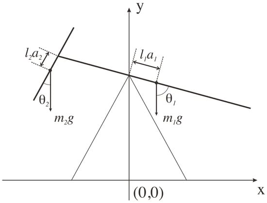
Figure 1. Sketch of the swinging sticks pendulum.

Our particular system is formed by two sticks of different lengths, pivoting about points displaced from their respective center of masses. The parameters of the system are the lengths, $l_1$ and $l_2$ (with $l_1>l_2$), and, without loss of generality, we set the masses $m_1\approx m_2=m$. The distance from the pivots to the respective center of masses are $a_1$ and $a_2$, respectively. Additionally, we set $a_1<{\displaystyle \frac{1}{2}}$ and $a_2\ll 1$. We will see below that additional restrictions are required for $a_1$, in order to get a unique stable equilibrium point.

We employ the angles ${\theta }_1$ and ${\theta }_2$ as generalized coordinates (see Figure 1), in order to analyze the motion of the sticks [12]. Thus, the Lagrangian for the longer stick can be written as

$$L_1=T_1-V_1$$

(1)

where $T_1$ ($V_1$) is the kinetic (potential) energy, and $I_{\mathrm{CM}}={\displaystyle \frac{m{l}^2}{12}}$, i.e., the moment of inertia for a stick rotating around its center of mass (CM). Explicitly, we can write

$$\begin{array}{cc}\hfill T_1& ={\displaystyle \frac{1}{2}}m({\dot{x}}_1^2+{\dot{y}}_1^2)+{\displaystyle \frac{1}{2}}{I}_{\mathrm{CM},1}{\dot{{\theta }_1}}^2\hfill \end{array}$$

(2)

and

$$\begin{array}{cc}\hfill V_1& =mg{l}_1\left[{\displaystyle \frac{1}{2}}+a_1(1-cos{\theta }_1)\right]\hfill \end{array}$$

(3)

where g is the gravity. The coordinates of the center of mass $x_1$ and $y_1$ can be written as

$$\begin{array}{cc}\hfill x_1& =a_1{l}_{1}sin{\theta }_1\hfill \\ \hfill y_1& ={\displaystyle \frac{l_1}{2}}+a_1{l}_1(1-cos{\theta }_1).\hfill \end{array}$$

(4)

Thus $L_1$ results in

$$\begin{array}{cc}\hfill L_1& ={\displaystyle \frac{1}{2}}m({\dot{x}}_1^2+{\dot{y}}_1^2)+{\displaystyle \frac{1}{2}}{I}_{\mathrm{CM},1}{\dot{{\theta }_1}}^2-mg{l}_1\left[{\displaystyle \frac{1}{2}}+a_1(1-cos{\theta }_1)\right].\hfill \end{array}$$

(5)

Replacing the velocity of the CM

$$\begin{array}{cc}\hfill {\dot{x}}_1& =a_1{l}_{1}cos{\theta }_1\dot{{\theta }_1}\hfill \\ \hfill {\dot{y}}_1& =a_1{l}_{1}sin{\theta }_1\dot{{\theta }_1},\hfill \end{array}$$

(6)

we can finally write

$$L_1\begin{array}{c}={\displaystyle \frac{1}{2}}m{l}_1^2{a}_1^2{\dot{{\theta }_1}}^2+{\displaystyle \frac{1}{2}}{I}_{\mathrm{CM},1}{\dot{{\theta }_1}}^2-mg{l}_1\left[{\displaystyle \frac{1}{2}}+a_1(1-cos{\theta }_1)\right]\hfill \\ ={\displaystyle \frac{1}{2}}m{l}_1^2\left(a_1^2+{\displaystyle \frac{1}{12}}\right){\dot{{\theta }_1}}^2-mg{l}_1\left[{\displaystyle \frac{1}{2}}+a_1(1-cos{\theta }_1)\right].\hfill \end{array}$$

(7)

For the shorter stick, we have

$$L_2=T_2-V_2,$$

(8)

where $T_2$ ($V_2$) is the kinetic (potential) energy. Explicitly, we can write for $T_2$

$$\begin{array}{cc}\hfill T_2& ={\displaystyle \frac{1}{2}}m({\dot{x}}_2^2+{\dot{y}}_2^2)+{\displaystyle \frac{1}{2}}{I}_{\mathrm{CM},2}{\dot{{\theta }_2}}^2.\hfill \end{array}$$

(9)

Using the coordinates of the CM,

$$\begin{array}{cc}\hfill x_2& =-l_1\left({\displaystyle \frac{1}{2}}-a_1\right)sin{\theta }_1-l_2{a}_{2}sin{\theta }_2\hfill \\ \hfill y_2& =l_1\left({\displaystyle \frac{1}{2}}+a_1\right)+l_1\left({\displaystyle \frac{1}{2}}-a_1\right)cos{\theta }_1-l_2{a}_{2}cos{\theta }_2\hfill \end{array}$$

(10)

the velocity becomes

$$\begin{array}{cc}\hfill {\dot{x}}_2& =-l_1\left({\displaystyle \frac{1}{2}}-a_1\right)cos{\theta }_1\dot{{\theta }_1}-l_2{a}_{2}cos{\theta }_2\dot{{\theta }_2}\hfill \end{array}$$

(11)

$$\begin{array}{cc}\hfill {\dot{y}}_2& =-l_1\left({\displaystyle \frac{1}{2}}-a_1\right)sin{\theta }_1\dot{{\theta }_1}+l_2{a}_{2}sin{\theta }_2\dot{{\theta }_2}.\hfill \end{array}$$

(12)

Finally $T_2$ is

$$T_2\begin{array}{c}={\displaystyle \frac{1}{2}}m\left[l_1^2{\left({\displaystyle \frac{1}{2}}-a_1\right)}^2{\dot{{\theta }_1}}^2+l_2^2{a}_2^2{\dot{{\theta }_2}}^2+2l_1{l}_2\left({\displaystyle \frac{1}{2}}-a_1\right)a_{2}cos({\theta }_1+{\theta }_2)\dot{{\theta }_1}\dot{{\theta }_2}\right]\hfill \\ +{\displaystyle \frac{1}{2}}{I}_{\mathrm{CM},2}{\dot{{\theta }_2}}^2.\hfill \end{array}$$

(13)

Simplifying, we have

$$T_2\begin{array}{c}={\displaystyle \frac{1}{2}}m{l}_1^2{\left({\displaystyle \frac{1}{2}}-a_1\right)}^2{\dot{{\theta }_1}}^2+{\displaystyle \frac{1}{24}}m{l}_2^2{\dot{{\theta }_2}}^2\hfill \\ +m{l}_1{l}_2\left({\displaystyle \frac{1}{2}}-a_1\right)a_{2}cos({\theta }_1+{\theta }_2)\dot{{\theta }_1}\dot{{\theta }_2},\hfill \end{array}$$

(14)

where we have neglected terms of the order $a_2^2$, since $a_2\ll 1$. For the potential energy $V_2$, we can write

$$\begin{array}{cc}\hfill V_2& =mg\left[l_1\left({\displaystyle \frac{1}{2}}+a_1\right)+l_1\left({\displaystyle \frac{1}{2}}-a_1\right)cos{\theta }_1-l_2{a}_{2}cos{\theta }_2\right].\hfill \end{array}$$

Likewise, the Lagrangian $L_2$ can then be written as

$$L_2\begin{array}{c}={\displaystyle \frac{1}{2}}m{l}_1^2{\left({\displaystyle \frac{1}{2}}-a_1\right)}^2{\dot{{\theta }_1}}^2+{\displaystyle \frac{1}{24}}m{l}_2^2{\dot{{\theta }_2}}^2\hfill \\ +m{l}_1{l}_2\left({\displaystyle \frac{1}{2}}-a_1\right)a_{2}cos({\theta }_1+{\theta }_2)\dot{{\theta }_1}\dot{{\theta }_2}\hfill \\ -mg\left[l_1\left({\displaystyle \frac{1}{2}}+a_1\right)+l_1\left({\displaystyle \frac{1}{2}}-a_1\right)cos{\theta }_1-l_2{a}_{2}cos{\theta }_2\right].\hfill \end{array}$$

(15)

We can then write the Lagrangian of the system $L=L_1+L_2$ as

$$\begin{array}{cc}\hfill L& ={\displaystyle \frac{1}{2}}m{l}_1^2\left(a_1^2+{\displaystyle \frac{1}{12}}\right){\dot{{\theta }_1}}^2+{\displaystyle \frac{1}{2}}m{l}_1^2{\left({\displaystyle \frac{1}{2}}-a_1\right)}^2{\dot{{\theta }_1}}^2+{\displaystyle \frac{1}{24}}m{l}_2^2{\dot{{\theta }_2}}^2\hfill \end{array}$$

$$\begin{array}{c}+m{l}_1{l}_2\left({\displaystyle \frac{1}{2}}-a_1\right)a_{2}cos({\theta }_1+{\theta }_2)\dot{{\theta }_1}\dot{{\theta }_2}\hfill \end{array}$$

(16)

$$\begin{array}{c}-mg{l}_1\left[{\displaystyle \frac{1}{2}}+a_1(1-cos{\theta }_1)\right]\hfill \end{array}$$

(17)

$$\begin{array}{c}-mg\left[l_1\left({\displaystyle \frac{1}{2}}+a_1\right)+l_1\left({\displaystyle \frac{1}{2}}-a_1\right)cos{\theta }_1-l_2{a}_{2}cos{\theta }_2\right].\hfill \end{array}$$

(18)

Let us analyze the potential energy, which can be written as

$$\begin{array}{cc}\hfill V& =mg{l}_1\left(1+{\displaystyle \frac{cos{\theta }_1}{2}}\right)+2mg{l}_1{a}_1(1-cos{\theta }_1)-mg{l}_2{a}_{2}cos{\theta }_2+V_0,\hfill \end{array}$$

(19)

to find the equilibrium positions. It is convenient to choose $V_0$ so that the potential energy of the pendulum is zero in a stable equilibrium position (see next). Equilibrium configurations of the system occur when $V=V({\theta }_1,{\theta }_2)$ is stationary with respect to ${\theta }_1$ and ${\theta }_2$, i.e., where the gradient of the potential vanishes $\overrightarrow{\nabla }V({\theta }_1,{\theta }_2)=\overrightarrow{0}$. Explicitly, we can write

$$\begin{array}{c}\hfill {\displaystyle \frac{\partial V}{\partial {\theta }_1}}={\displaystyle \frac{mg{l}_1}{2}}\left(4a_1-1\right)sin{\theta }_1\mathrm{and}{\displaystyle \frac{\partial V}{\partial {\theta }_2}}=mg{l}_2{a}_{2}sin{\theta }_2.\end{array}$$

(20)

The four equilibrium configurations are $({\theta }_1,{\theta }_2)=(0,0)$, $({\theta }_1,{\theta }_2)=(0,\pi )$, $({\theta }_1,{\theta }_2)=(\pi ,0)$ and $({\theta }_1,{\theta }_2)=(\pi ,\pi )$. In order to establish the nature of these equilibrium points, i.e., if they correspond to a situation of an equilibrium stable, unstable or neutral, we compute the Hessian matrix

$$\begin{array}{c}\hfill H=\left(\begin{array}{cc}{V}_{{\theta }_1{\theta }_1}& V_{{\theta }_1{\theta }_2}\\ V_{{\theta }_2{\theta }_1}& V_{{\theta }_2{\theta }_2}\end{array}\right),\end{array}$$

(21)

where $V_{{\theta }_1{\theta }_1}={\displaystyle \frac{{\partial }^{2}V}{\partial {\theta }_1^2}}$, $V_{{\theta }_2{\theta }_2}={\displaystyle \frac{{\partial }^{2}V}{\partial {\theta }_2^2}}$, and $V_{{\theta }_1{\theta }_2}=V_{{\theta }_2{\theta }_1}={\displaystyle \frac{{\partial }^{2}V}{\partial {\theta }_1\partial {\theta }_2}}$. Plugging the second order partial derivatives in H results in

$$\begin{array}{c}\hfill H=\left(\begin{array}{cc}{\displaystyle \frac{mg{l}_1}{2}}(4a_1-1)cos{\theta }_1& 0\\ 0& mg{l}_2{a}_{2}cos{\theta }_2\end{array}\right).\end{array}$$

(22)

In our setup, we have set $a_1<{\displaystyle \frac{1}{2}}$ and $a_2>0$, then, in order to have only one stable equilibrium point in $({\theta }_1,{\theta }_2)=(0,0)$, it is necessary that $a_1>{\displaystyle \frac{1}{4}}$. This can be verified by calculating the eigenvalues ${\lambda }_1,{\lambda }_2$ of H at the four equilibrium point pairs and requiring that both are strictly positive [14,15].

The potential energies of these four cases $V=E_i$ (with $i=1,\dots$, 4) can be written as:

$$\begin{array}{cc}\hfill E_1& =mg\left({\displaystyle \frac{3}{2}}{l}_1-a_2{l}_2\right)\hfill \end{array}$$

(23)

$$\begin{array}{cc}\hfill E_2& =mg\left({\displaystyle \frac{3}{2}}{l}_1+a_2{l}_2\right)\hfill \end{array}$$

(24)

$$\begin{array}{cc}\hfill E_3& =mg\left[\left(4a_1+{\displaystyle \frac{1}{2}}\right)l_1-a_2{l}_2\right]\hfill \end{array}$$

(25)

$$\begin{array}{cc}\hfill E_4& =mg\left[\left(4a_1+{\displaystyle \frac{1}{2}}\right)l_1+a_2{l}_2\right].\hfill \end{array}$$

(26)

We can then write the potential $V=V({\theta }_1,{\theta }_2)$ as

$$\begin{array}{cc}\hfill V({\theta }_1,{\theta }_2)& ={\displaystyle \frac{1}{2}}\left[(E_1-E_3)cos{\theta }_1-(E_2-E_1)cos{\theta }_2+(E_2+E_3-2E_1)\right],\hfill \end{array}$$

where we have chosen $V_0$ in such a way that $V(0,0)=0$. The total kinetic energy of the system can be written as

$$\begin{array}{cc}\hfill T& =k_1{\dot{{\theta }_1}}^2+2k_{2}cos({\theta }_1+{\theta }_2)\dot{{\theta }_1}\dot{{\theta }_2}+k_3{\dot{{\theta }_2}}^2\hfill \end{array}$$

(27)

where

$$\begin{array}{cc}\hfill k_1& ={\displaystyle \frac{1}{2}}m{l}_1^2\left[\left(a_1^2+{\displaystyle \frac{1}{12}}\right)+{\left({\displaystyle \frac{1}{2}}-a_1\right)}^2\right]\hfill \end{array}$$

(28)

$$\begin{array}{cc}\hfill k_2& ={\displaystyle \frac{1}{2}}m{l}_1{l}_2\left({\displaystyle \frac{1}{2}}-a_1\right)a_2\hfill \end{array}$$

(29)

$$\begin{array}{cc}\hfill k_3& ={\displaystyle \frac{1}{24}}m{l}_2^2.\hfill \end{array}$$

(30)

From the Lagrangian L we can obtain the Euler–Lagrange (EL) equations for ${\theta }_1$ and ${\theta }_2$ as

$$\begin{array}{cc}\hfill {\displaystyle \frac{d}{dt}}{\displaystyle \frac{\partial L}{\partial \dot{{\theta }_1}}}& ={\displaystyle \frac{\partial L}{\partial {\theta }_1}}\hfill \end{array}$$

(31)

$$\begin{array}{cc}\hfill {\displaystyle \frac{d}{dt}}{\displaystyle \frac{\partial L}{\partial \dot{{\theta }_2}}}& ={\displaystyle \frac{\partial L}{\partial {\theta }_2}}.\hfill \end{array}$$

(32)

Let us first compute the partial derivatives with respect to $\dot{{\theta }_1}$ and $\dot{{\theta }_2}$, i.e.,

$$\begin{array}{cc}\hfill {\displaystyle \frac{\partial L}{\partial \dot{{\theta }_1}}}& =2k_1\dot{{\theta }_1}+2k_{2}cos({\theta }_1+{\theta }_2)\dot{{\theta }_2}\hfill \end{array}$$

(33)

$$\begin{array}{cc}\hfill {\displaystyle \frac{\partial L}{\partial \dot{{\theta }_2}}}& =2k_3\dot{{\theta }_2}+2k_{2}cos({\theta }_1+{\theta }_2)\dot{{\theta }_1}.\hfill \end{array}$$

(34)

Then, let us calculate the left-hand side of the EL equations

$$\begin{array}{cc}\hfill {\displaystyle \frac{d}{dt}}{\displaystyle \frac{\partial L}{\partial \dot{{\theta }_1}}}& =2k_1\ddot{{\theta }_1}-2k_{2}sin({\theta }_1+{\theta }_2)(\dot{{\theta }_1}+\dot{{\theta }_2})\dot{{\theta }_2}+2k_{2}cos({\theta }_1+{\theta }_2)\ddot{{\theta }_2}\hfill \end{array}$$

(35)

$$\begin{array}{cc}\hfill {\displaystyle \frac{d}{dt}}{\displaystyle \frac{\partial L}{\partial \dot{{\theta }_2}}}& =2k_3\ddot{{\theta }_2}-2k_{2}sin({\theta }_1+{\theta }_2)(\dot{{\theta }_1}+\dot{{\theta }_2})\dot{{\theta }_1}+2k_{2}cos({\theta }_1+{\theta }_2)\ddot{{\theta }_1}.\hfill \end{array}$$

(36)

Now let us work with the right-hand side of the EL equations to obtain

$$\begin{array}{cc}\hfill {\displaystyle \frac{\partial L}{\partial {\theta }_1}}& =-2k_{2}sin({\theta }_1+{\theta }_2)\dot{{\theta }_1}\dot{{\theta }_2}-mg{l}_1\left(2a_1-{\displaystyle \frac{1}{2}}\right)sin{\theta }_1\hfill \end{array}$$

(37)

$$\begin{array}{cc}\hfill {\displaystyle \frac{\partial L}{\partial {\theta }_2}}& =-2k_{2}sin({\theta }_1+{\theta }_2)\dot{{\theta }_1}\dot{{\theta }_2}-mg{l}_2{a}_{2}sin{\theta }_2.\hfill \end{array}$$

(38)

Finally, the EL equations result in

$$\begin{array}{c}\hfill 2k_1\ddot{{\theta }_1}-2k_{2}sin({\theta }_1+{\theta }_2)(\dot{{\theta }_1}+\dot{{\theta }_2})\dot{{\theta }_2}+2k_{2}cos({\theta }_1+{\theta }_2)\ddot{{\theta }_2}\\ \hfill +2k_{2}sin({\theta }_1+{\theta }_2)\dot{{\theta }_1}\dot{{\theta }_2}+mg{l}_1\left(2a_1-{\displaystyle \frac{1}{2}}\right)sin{\theta }_1& =0\hfill \end{array}$$

(39)

$$\begin{array}{c}\hfill 2k_3\ddot{{\theta }_2}-2k_{2}sin({\theta }_1+{\theta }_2)(\dot{{\theta }_1}+\dot{{\theta }_2})\dot{{\theta }_1}+2k_{2}cos({\theta }_1+{\theta }_2)\ddot{{\theta }_1}\\ \hfill +2k_{2}sin({\theta }_1+{\theta }_2)\dot{{\theta }_1}\dot{{\theta }_2}+mg{l}_2{a}_{2}sin{\theta }_2& =0.\hfill \end{array}$$

(40)

3. Dynamical System

We can rewrite the dynamical system, derived from the second-order EL equations of motion, Equations (39) and (40), as a set of first-order differential equations as

$$\begin{array}{cc}\hfill \dot{{\theta }_1}=& {\omega }_1\end{array}$$

(41)

$$\begin{array}{cc}\hfill \dot{{\theta }_2}=& {\omega }_2\end{array}$$

(42)

$$\dot{{\omega }_1}=\begin{array}{c}{\displaystyle \frac{mg\left[(\frac{1}{4}-a_1)k_3{l}_{1}sin\left({\theta }_1\right)+\frac{1}{2}{k}_2{a}_2{l}_{2}sin\left({\theta }_2\right)cos({\theta }_1+{\theta }_2)\right]}{k_1{k}_3-k_2^2{cos}^2({\theta }_1+{\theta }_2)}}\\ +{\displaystyle \frac{k_2\left[k_3{\omega }_2^{2}sin({\theta }_1+{\theta }_2)-\frac{1}{2}{k}_2{\omega }_1^{2}sin\left(2({\theta }_1+{\theta }_2)\right)\right]}{k_1{k}_3-k_2^2{cos}^2({\theta }_1+{\theta }_2)}}\end{array}$$

(43)

$$\dot{{\omega }_2}=\begin{array}{c}{\displaystyle \frac{mg\left[(a_1-\frac{1}{4})k_2{l}_{1}sin\left({\theta }_1\right)cos({\theta }_1+{\theta }_2)-\frac{1}{2}{k}_1{a}_2{l}_{2}sin\left({\theta }_2\right)\right]}{k_1{k}_3-k_2^2{cos}^2({\theta }_1+{\theta }_2)}}\\ +{\displaystyle \frac{k_2\left[k_1{\omega }_1^{2}sin({\theta }_1+{\theta }_2)-\frac{1}{2}{k}_2{\omega }_2^{2}sin\left(2({\theta }_1+{\theta }_2)\right)\right]}{k_1{k}_3-k_2^2{cos}^2({\theta }_1+{\theta }_2)}}.\end{array}$$

(44)

Therefore, our study addresses an autonomous system defined by two angles (${\theta }_1$ and ${\theta }_2$) and two angular velocities (${\omega }_1$ and ${\omega }_2$), which together create a four-dimensional state space. The system has the following fixed points

$$({\theta }_1,{\theta }_2,{\omega }_1,{\omega }_2)=(0,0,0,0),(0,\pi ,0,0),(\pi ,0,0,0),(\pi ,\pi ,0,0).$$

(45)

Note that these fixed points correspond to the equilibrium configurations derived in Section 2. The local stability of these points is calculated from the eigenvalues of the Jacobian matrix, ${\displaystyle \frac{d\overrightarrow{f}}{d\overrightarrow{x}}}$, valued at each fixed point. Where $\overrightarrow{f}=[\dot{{\theta }_1},\dot{{\theta }_2},\dot{{\omega }_1},\dot{{\omega }_2}]$ and $\overrightarrow{x}=[{\theta }_1,{\theta }_2,{\omega }_1,{\omega }_2]$.

As an example, we consider the following data: $m=0.1$ kg, $l_1=0.15$ m, $l_2=0.1$ m, $g=9.81$ m/s², $a_1=0.4$, and $a_2=0.01$. Thus, we can compute the eigenvalues as follows:

$$\begin{gathered} \mathrm{For}{\mu }_1=({\theta }_1,{\theta }_2,{\omega }_1,{\omega }_2)=(0,0,0,0),\mathrm{the}\mathrm{eigenvalues}\mathrm{are} \\ {\lambda }_1=0+8.80066i,{\lambda }_2=0-8.80066i, \\ {\lambda }_3=0+3.43102i,{\lambda }_4=0-3.43102i \end{gathered}$$

(46)

$$\begin{gathered} \mathrm{For}{\mu }_2=({\theta }_1,{\theta }_2,{\omega }_1,{\omega }_2)=(0,\pi ,0,0),\mathrm{the}\mathrm{eigenvalues}\mathrm{are} \\ {\lambda }_1=0+8.8006i,{\lambda }_2=0-8.80066i, \\ {\lambda }_3=-3.43105,{\lambda }_4=3.43105 \end{gathered}$$

(47)

$$\begin{gathered} \mathrm{For}{\mu }_3=({\theta }_1,{\theta }_2,{\omega }_1,{\omega }_2)=(\pi ,0,0,0),\mathrm{the}\mathrm{eigenvalues}\mathrm{are} \\ {\lambda }_1=-8.8006,{\lambda }_2=8.80066, \\ {\lambda }_3=0+3.43105i,{\lambda }_4=0-3.43105i \end{gathered}$$

(48)

$$\begin{gathered} \mathrm{For}{\mu }_4=({\theta }_1,{\theta }_2,{\omega }_1,{\omega }_2)=(\pi ,\pi ,0,0),\mathrm{the}\mathrm{eigenvalues}\mathrm{are} \\ {\lambda }_1=-8.8006,{\lambda }_2=8.80066, \\ {\lambda }_3=3.43105,{\lambda }_4=-3.43105. \end{gathered}$$

(49)

If all eigenvalues of the Jacobian matrix are purely imaginary and nonzero, then the corresponding fixed point is referred to as a center. Therefore, the fixed point ${\mu }_1$ is a center (a non-hyperbolic point), while ${\mu }_2$, ${\mu }_3$, and ${\mu }_4$ are unstable fixed points. A fixed point is unstable if one or more of the eigenvalues of the Jacobian matrix have positive real parts. If a center fixed point is perturbed, trajectories around the fixed point are generated. On the other hand, if an unstable fixed point is disturbed, the perturbation causes the trajectories to move away from the fixed point. This result aligns with the conclusion drawn above using the Hessian matrix.

4. Numerical Scheme

The dynamical system outlined in Equations (41)–(44) does not possess analytical solutions. Consequently, it is necessary to employ numerical methods to integrate them. In this context, the Bulirsch–Stoer method, a variation of the extrapolated modified midpoint, has been used for the analysis [16].

The system (41)–(44) can be written as

$${\displaystyle \frac{d\overrightarrow{x}}{dt}}=\overrightarrow{f}\left(\overrightarrow{x}\right),\overrightarrow{x}\left(0\right)={\overrightarrow{x}}_0,$$

(50)

where $\overrightarrow{x}=({\theta }_1,{\theta }_2,{\omega }_1,{\omega }_2)$. The time domain $[t_0,t_f]$ is discretized using a grid $(t_0,t_0+\Delta t,t_0+2\Delta t,...)$. The objective is to advance the solution from a generic grid point $t_n$ to $t_{n+1}=t_n+\Delta t$. Then, the Bulirsch–Stoer method starts from the modified midpoint method

$$\begin{array}{cc}\hfill {\overrightarrow{z}}_0=& {\overrightarrow{x}}_n=\overrightarrow{x}(t_n,h)\end{array}$$

(51)

$$\begin{array}{cc}\hfill {\overrightarrow{z}}_1=& {\overrightarrow{z}}_0+h\overrightarrow{f}(t_n,{\overrightarrow{x}}_0)\end{array}$$

(52)

$$\begin{array}{cc}\hfill {\overrightarrow{z}}_i=& {\overrightarrow{z}}_{i-2}+2h\overrightarrow{f}(t_n+(i-1)h,{\overrightarrow{x}}_{i-1}),i=2,...,M\end{array}$$

(53)

$$\begin{array}{cc}\hfill {\overrightarrow{x}}_{n+1}=\overrightarrow{x}(t_{n+1},h)=& 0.5\left[{\overrightarrow{z}}_{M-1}+{\overrightarrow{z}}_M+h\overrightarrow{f}(t_n+\Delta t{\overrightarrow{z}}_M)\right],\end{array}$$

(54)

where $h=\Delta t/M$, and M is the number of sub-steps inside the interval [$t_n,t_n+\Delta t]$. A table for $\overrightarrow{x}(t_{n+1},h)$ is developed for the chosen number of values of M, and the $\overrightarrow{x}(t_{n+1},h)$ values are successively extrapolated to higher and higher orders as follows [17]

$${\overrightarrow{y}}_j^k={\overrightarrow{y}}_j^{k-1}+{\displaystyle \frac{{\overrightarrow{y}}_j^{k-1}-{\overrightarrow{y}}_{j-1}^{k-1}}{{\left(\frac{n_j}{n_{j-k+1}}\right)}^2-1}},k=2,3,...$$

(55)

where ${\overrightarrow{y}}_j^1=\overrightarrow{x}(\Delta t,h_j)$, $j=1,2,3,...$, and $M=2j$.

5. Motion at Low Energy

When the total energy of the system is low, the nonlinear terms in Equations (41)–(44) can be neglected, and the pendulum will oscillate with a small amplitude around the stable equilibrium point. Accordingly, Equations (39) and (40) can be linearized by employing small-angle approximations and omitting nonlinear terms, resulting in the following linear system of ordinary differential equations:

$$2k_1\ddot{{\theta }_1}+2k_2\ddot{{\theta }_2}+mg{l}_1\left(2a_1-{\displaystyle \frac{1}{2}}\right){\theta }_1=0$$

(56)

$$2k_3\ddot{{\theta }_2}+2k_2\ddot{{\theta }_1}+mg{l}_2{a}_2{\theta }_2=0.$$

(57)

The normal modes of oscillation refer to the motions in which the angles ${\theta }_1$ and ${\theta }_2$ vary harmonically in time with the same frequency and phase, albeit not necessarily with the same amplitude, i.e.,

$${\theta }_1=A_1{e}^{i\omega t},{\theta }_2=A_2{e}^{i\omega t}.$$

(58)

Upon substituting harmonic solutions into the linearized system (56) and (57), two normal or characteristic angular velocities (or frequencies), denoted as ${\omega }_{+}$ and ${\omega }_{-}$, are identified, representing the fast and slow modes of oscillation:

$${\omega }_{\pm }^2={\displaystyle \frac{k_1{k}_5+k_3{k}_4\pm \sqrt{{(k_1{k}_5-k_3{k}_4)}^2+4k_2^2{k}_4{k}_5}}{2(k_1{k}_3-k_2^2)}},$$

(59)

where

$$\begin{array}{cc}\hfill k_4& =mg{l}_1\left(a_1-{\displaystyle \frac{1}{4}}\right),\hfill \end{array}$$

(60)

$$\begin{array}{cc}\hfill k_5& ={\displaystyle \frac{mg{l}_2{a}_2}{2}}.\hfill \end{array}$$

(61)

On introducing the normal modes, Equations (58) and (59), into the governing Equations (56) and (57), the relation between the amplitude factors $A_1$ and $A_2$ for the harmonic motions is obtained:

$${\left({\displaystyle \frac{A_1}{A_2}}\right)}_{\pm }={\displaystyle \frac{k_2{\omega }_{\pm }^2}{k_4-k_1{\omega }_{\pm }^2}}={\displaystyle \frac{k_5-k_3{\omega }_{\pm }^2}{k_2{\omega }_{\pm }^2}}.$$

(62)

When ${\displaystyle \frac{A_1}{A_2}}>0$, the two sticks oscillate in the same direction; when ${\displaystyle \frac{A_1}{A_2}}<0$, they move in opposite directions. For both modes, fast and slow, we identified a family of non-trivial solutions $A_{1\pm }=A_1\left(A_{2\pm }\right)$. Consequently, the amplitude of the normal mode is not uniquely determined; this occurs because the governing system of ordinary differential equations is homogeneous and linear [18].

Among the four fixed points, only ${\mu }_1$ can generate motion at low energies. For the other three fixed points, which are unstable, movement is not limited to small disturbances. Several numerical tests are performed, using the Bulirsch–Stoer method described above, to analyze the behavior of the system around the fixed point $({\theta }_1,{\theta }_2,{\omega }_1,{\omega }_2)=(0,0,0,0)$. The following parameters are set in the tests: $m=0.1\mathrm{kg},l_1=0.15\mathrm{m},l_2=0.1\mathrm{m},g=9.81{\mathrm{m}/\mathrm{s}}^2,a_1=0.4,a_2=0.01$. The system at this fixed point has an energy $E_1=0.219744$ J. Energy conservation is confirmed for all time steps, with a tolerance of less than ${10}^{-12}$. The dynamics of the system described by Equations (41)–(44) in the vicinity of the fixed point ${\mu }_1=(0,0,0,0)$ is examined. This fixed point acts as a center; consequently, a small perturbation applied as an initial condition is expected to result in a motion around it. Four tests are conducted using different initial conditions.

For the first test, the initial condition is ${({\theta }_1,{\theta }_2,{\omega }_1,{\omega }_2)}_0=(0.01,0,0,0)$, which corresponds to an energy $E=0.219746207232$ J. Figure 2 and Figure 3 illustrate the temporal evolution of $({\theta }_1,{\omega }_1)$ and $({\theta }_2,{\omega }_2)$, respectively.

Figure 2. Numerical solution for Equations (41)–(44) for ${\theta }_1\left(t\right)$ (top panel) and ${\omega }_1\left(t\right)$ (bottom panel). The initial condition is ${({\theta }_1,{\theta }_2,{\omega }_1,{\omega }_2)}_0=(0.01,0,0,0)$. The simulation duration is 20 s. The first rod exhibits periodic motion with a single frequency of approximately $f_{+}\cong 1.4$ 1/s.

Figure 3. Numerical solution for Equations (41) and (44) for ${\theta }_2\left(t\right)$ (top panel) and ${\omega }_2\left(t\right)$ (bottom panel). The initial condition is ${({\theta }_1,{\theta }_2,{\omega }_1,{\omega }_2)}_0=(0.01,0,0,0)$. The simulation duration is 20 s. The second rod displays quasiperiodic motion with two frequencies $f_{+}\cong 1.4$ 1/s and $f_{-}\cong 0.55$ 1/s.

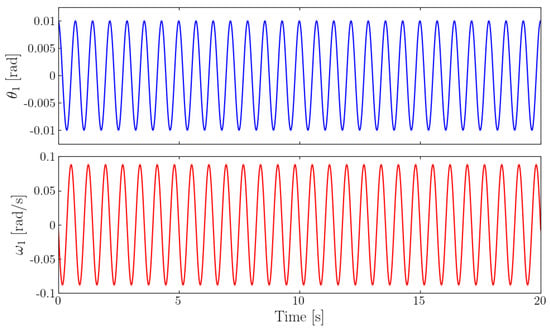
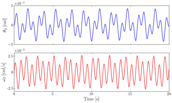
To describe the frequencies involved in the motion, the fast Fourier transform (FFT) is applied to both ${\theta }_1$ and ${\theta }_2$. For ${\theta }_1$, only the frequency $f_{+}\cong 1.4$ 1/s is present and supports the motion. In contrast, ${\theta }_2$ reveals two frequencies: $f_{+}\cong 1.4$ 1/s and $f_{-}\cong 0.55$ 1/s. These results are illustrated in Figure 4.

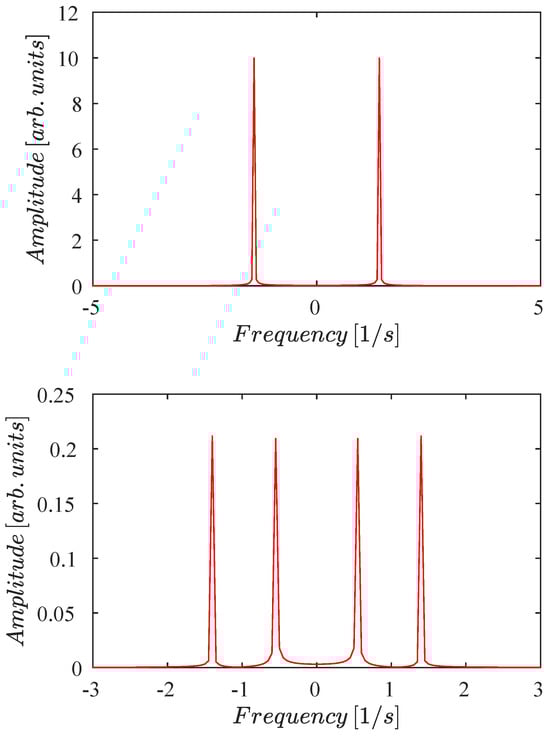
Figure 4. Fast Fourier transform for test 1. The initial condition is ${({\theta }_1,{\theta }_2,{\omega }_1,{\omega }_2)}_0=(0.01,0,0,0)$. (Top panel) For ${\theta }_1$, only a single frequency $f_{+}\cong 1.4$ 1/s is observed. (Bottom panel) For ${\theta }_2$, two frequencies $f_{+}\cong 1.4$ 1/s and $f_{-}\cong 0.55$ 1/s are clearly visible.

Another tool for analyzing the system’s dynamics is Poincaré maps [19,20]. To construct a Poincaré map for a solution of the equations system (41)–(44), the $f_{+}$ frequency is used as the sampling frequency; therefore, the Poincaré map is made up of values of ${\theta }_1\left(t\right)$ and ${\theta }_2\left(t\right)$ obtained for integer multiples of the period $1/f_{+}$, then points satisfying $t=n/f_{+}$ with $n=1,2,3,\dots$. After obtaining the sampled data series for ${\theta }_1$ and ${\theta }_2$, the FFT is applied. The FFT for ${\theta }_1$ shows that there are no other frequencies involved in the motion of ${\theta }_1$. However, for ${\theta }_2$, the FFT for the sampled series displays a frequency $f_{-}\cong 0.55$ 1/s. Figure 5 shows the Fourier transform for values of ${\theta }_1$ and ${\theta }_2$ captured at integer multiples of $1/f_{+}$. The upper figure displays the FFT for ${\theta }_1$ and the lower one for ${\theta }_2$. Also, the Poincaré map ${\omega }_2$ vs ${\theta }_2$ is displayed in Figure 6, which is a closed curve that depends on a single frequency $f_{-}$.

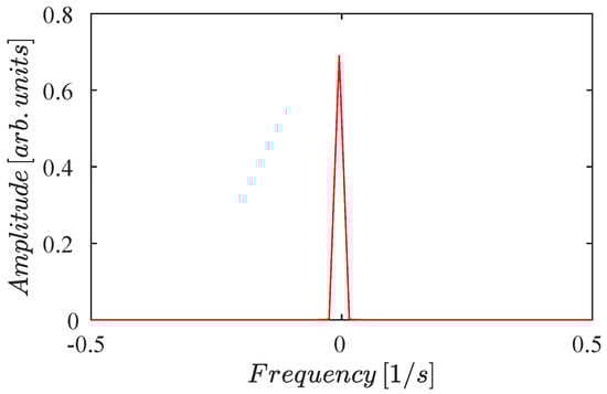
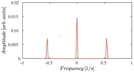
Figure 5. Fast Fourier transform for test 1 using Poincaré maps. The initial condition is ${({\theta }_1,{\theta }_2,{\omega }_1,{\omega }_2)}_0=(0.01,0,0,0)$. The Poincaré maps are obtained at a sampling frequency of $1/f_{+}$. (Top panel) For ${\theta }_1$, there are no frequencies involved. (Bottom panel) For ${\theta }_2$, only a single frequency $f_{-}\cong 0.55$ 1/s is visible.

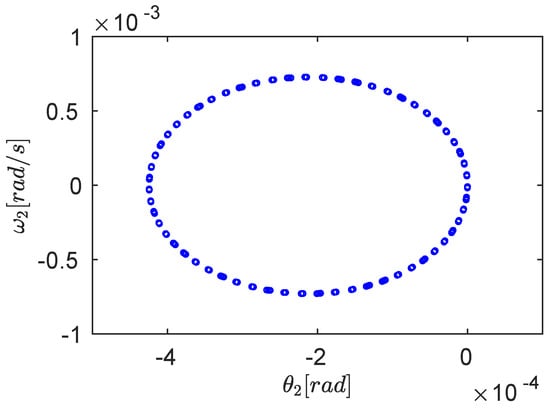
Figure 6. Poincaré map made up of values of ${\theta }_2$ and ${\omega }_2$ obtained for integer multiples of $1/f_{+}$. Thus, points satisfying $t=n/f_{+}$ with $n\in Z^{+}$, where $Z^{+}$ are the positive integer numbers. The simulation duration is 100 s. The only frequency is $f_{-}$.

The second test begins with the initial conditions ${({\theta }_1,{\theta }_2,{\omega }_1,{\omega }_2)}_0=(0,0.01,0,0)$. The associated energy is $E=0.21974404905$ J. In this scenario, the motion of ${\theta }_1$ is characterized by two frequencies, $f_{+}\cong 1.4$ 1/s and $f_{-}\cong 0.55$ 1/s. In contrast, the motion of ${\theta }_2$ is governed solely by a single frequency of $f_{-}\cong 0.55$ 1/s. The FFT results are shown in Figure 7.

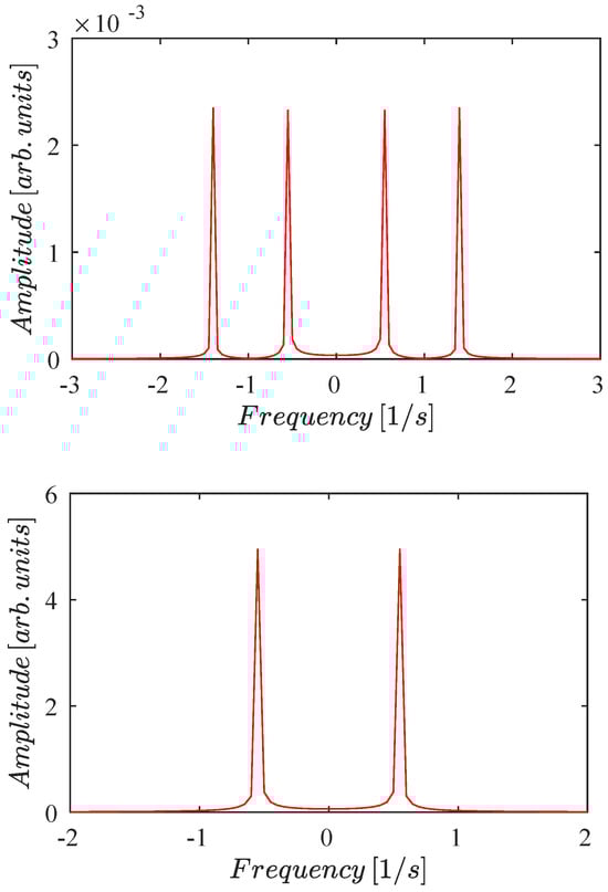
Figure 7. Fast Fourier transform for test 2. The initial condition is ${({\theta }_1,{\theta }_2,{\omega }_1,{\omega }_2)}_0=(0,0.01,0,0)$. (Top panel) For ${\theta }_1$, there are two frequencies $f_{+}\cong 1.4$ 1/s and $f_{-}\cong 0.55$ 1/s. (Bottom panel) For ${\theta }_2$, only one frequency $f_{-}\cong 0.55$ 1/s is present.

The initial condition for the third test is set to ${({\theta }_1,{\theta }_2,{\omega }_1,{\omega }_2)}_0=(0,0,0.01,0)$, which corresponds to $E=0.2197440285$ J. In this case, the initial perturbation applies only to ${\omega }_1$. The FFT is used to determine the frequencies supporting the system dynamics. For ${\theta }_1$, only the frequency $f_{+}\cong 1.4$ 1/s is obtained from the numerical results. In contrast, for ${\theta }_2$ the numerical data reveal two frequencies: $f_{+}\cong 1.4$ 1/s and $f_{-}\cong 0.55$ 1/s.

The fourth test uses the following initial condition ${({\theta }_1,{\theta }_2,{\omega }_1,{\omega }_2)}_0=(0,0,0,0.01)$. Therefore, the system has an energy $E=0.219744004167$ J. Then, a small initial perturbation affects only ${\omega }_2$. For ${\theta }_1$, the FFT determines two frequencies $f_{+}\cong 1.4$ 1/s and $f_{-}\cong 0.55$ 1/s, and for ${\theta }_2$ only a single frequency $f_{-}\cong 0.55$ 1/s.

For all tests, the FFT algorithm provided by MATLAB (version 24.2 (R2024b)) is used [21]. The FFT by default uses a rectangular window whose length matches that of the signal. To verify the results, we have also used a Hanning window [22], obtaining the same frequencies. The resolution for all cases is set to $0.04995$.

At low energy, the frequencies of the motion can be obtained from Equation (59). For the same parameters used in the numerical tests, the calculated frequencies are $f_{+}={\displaystyle \frac{{\omega }_{+}}{2\pi }}\cong 1.4$ 1/s and $f_{-}\cong {\displaystyle \frac{{\omega }_{-}}{2\pi }}\cong 0.55$ 1/s. Note the high accuracy between the numerical and analytical values obtained.

In a low-energy scenario, the system dynamics can be described as the sum of normal modes. In the first test, the motion of ${\theta }_1$ is dictated exclusively by the mode with frequency $f_{+}$. In contrast, the motion of ${\theta }_2$ arises from a combination of two normal modes associated with the frequencies $f_{+}$ and $f_{-}$. For the second test, the dynamics of ${\theta }_1$ is given by the sum of two normal modes with frequencies $f_{+}$ and $f_{-}$, and the motion of ${\theta }_2$ depends only on one normal mode with frequency $f_{-}$. In the third test, behaviors consistent with those observed in the first case are noted. In contrast, the dynamic in the fourth test resembles that seen in the second test.

It is essential to recognize how the motion of the system is influenced by its initial conditions. When the initial perturbation affects either ${\theta }_1$ or ${\omega }_1$, the dynamics of the first stick exhibits a periodic motion determined by a single frequency. In contrast, the motion of the second stick is influenced by two frequencies. It is also observed that the amplitude of movement of the first stick is greater than that of the second stick. On the other hand, if a small initial perturbation is applied to ${\theta }_2$ or ${\omega }_2$, the motion of the second stick is governed by one frequency, while the motion of the first stick is affected by two frequencies. However, the movement amplitude of the second stick is greater than that of the first stick.

The quotient between $f_{+}$ and $f_{-}$ is an irrational number, indicating that the motion around the fixed point $({\theta }_1,{\theta }_2,{\omega }_1,{\omega }_2)=(0,0,0,0)$ is quasiperiodic [8,19]. To analytically describe the motion of the low-energy system, we can write ${\theta }_1$ and ${\theta }_2$ as the sum of the normal modes [23]:

$$\begin{array}{c}\hfill {\theta }_1\left(t\right)=A_{11}{e}^{i{\omega }_{+}t}+A_{12}{e}^{-i{\omega }_{+}t}+A_{13}{e}^{i{\omega }_{-}t}+A_{14}{e}^{-i{\omega }_{-}t},\end{array}$$

(63)

$$\begin{array}{c}\hfill {\theta }_2\left(t\right)=A_{21}{e}^{i{\omega }_{+}t}+A_{22}{e}^{-i{\omega }_{+}t}+A_{23}{e}^{i{\omega }_{-}t}+A_{24}{e}^{-i{\omega }_{-}t}.\end{array}$$

(64)

However, the coefficients $A_{ij}$ are related by Equation (62). Therefore, the previous equations results in

$$\begin{array}{c}\hfill {\theta }_1\left(t\right)=A_{11}{e}^{i{\omega }_{+}t}+A_{12}{e}^{-i{\omega }_{+}t}+A_{13}{e}^{i{\omega }_{-}t}+A_{14}{e}^{-i{\omega }_{-}t},\end{array}$$

(65)

$$\begin{array}{c}\hfill {\theta }_2\left(t\right)={\displaystyle \frac{k_4-k_1{\omega }_{+}^2}{k_2{\omega }_{+}^2}}\left(A_{11}{e}^{i{\omega }_{+}t}+A_{12}{e}^{-i{\omega }_{+}t}\right)+{\displaystyle \frac{k_4-k_1{\omega }_{-}^2}{k_2{\omega }_{-}^2}}\left(A_{13}{e}^{i{\omega }_{-}t}+A_{14}{e}^{-i{\omega }_{-}t}\right).\end{array}$$

(66)

These two equations and their derivatives, ${\omega }_1$ and ${\omega }_2$, form a system of four equations that allows us to determine $A_{11}$, $A_{12}$, $A_{13}$, and $A_{14}$. As a first example, we analyze the test with the initial conditions ${({\theta }_1,{\theta }_2,{\omega }_1,{\omega }_2)}_0=(0,0.01,0,0)$. We obtain $A_{11}=A_{12}=-2.35844333887164\times {10}^{-6}$, and $A_{13}=A_{14}=2.35844333887164\times {10}^{-6}$. Figure 8 and Figure 9 compare numerical data and analytical results. The blue line represents the analytical results, and the red points are the numerical data. In addition, we calculate the highest difference between the analytical and numerical results as the largest value of the difference $M_d=\left|N_v-A_v\right|$, the mean error $E_m=\left({\sum }_N(N_v-A_v)\right)/N$, and the standard deviation of the error $\sigma =\sqrt{\left({\sum }_N{(N_v-A_v-E_m)}^2\right)/N}$, where $N_v$ and $A_v$ are the numerical and analytical values of the data series, and N is the number of elements of the data series. For ${\theta }_1$, we find $M_d=2.5549\times {10}^{-9}$, $E_m=-2.8288\times {10}^{-11}$ and $\sigma =5.294\times {10}^{-22}$, and for ${\theta }_2$, we calculate $M_d=4.2191\times {10}^{-6}$, $E_m=-5.6381\times {10}^{-8}$ and $\sigma =9.3512\times {10}^{-19}$.

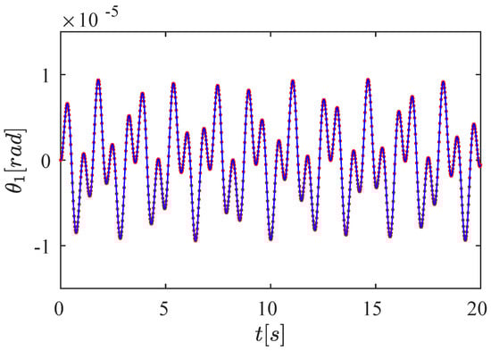
Figure 8. Analytical and numerical results for ${\theta }_1$ with initial condition ${({\theta }_1,{\theta }_2,{\omega }_1,{\omega }_2)}_0=(0,0.01,0,0)$. The blue line represents the analytical results, and the red points are the numerical data. The highest difference is $M_d=2.5549\times {10}^{-9}$, the mean error is $E_m=-2.8288\times {10}^{-11}$, and the standard deviation is $\sigma =5.294\times {10}^{-22}$. The numerical data show a high accuracy with the analytical results. The motion of ${\theta }_1$ shows two frequencies, $f_{+}\cong 1.4$ 1/s and $f_{-}\cong 0.55$ 1/s. The simulation duration is 20 s.

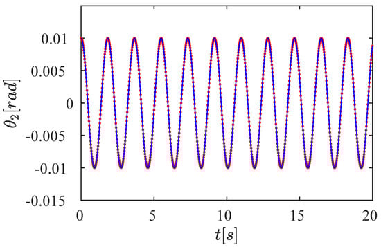
Figure 9. Analytical and numerical results for ${\theta }_2$ with initial condition ${({\theta }_1,{\theta }_2,{\omega }_1,{\omega }_2)}_0=(0,0.01,0,0)$. The blue line represents the analytical results, and the red points are the numerical data. The highest difference is $M_d=4.2191\times {10}^{-6}$, the mean error is $E_m=-5.6381\times {10}^{-8}$, and the standard deviation is $\sigma =9.3512\times {10}^{-19}$. The numerical results show a high accuracy with the theoretical data. For ${\theta }_2$, only one frequency, $f_{-}\cong 0.55$ 1/s, is present. The simulation duration is 20 s.

For this test, we evaluate that

$$|{\displaystyle \frac{\frac{k_4-k_1{\omega }_{+}^2}{k_2{\omega }_{+}^2}}{\frac{k_4-k_1{\omega }_{-}^2}{k_2{\omega }_{-}^2}}|}\ll 1.$$

(67)

This result implies that ${\theta }_2$ only depends on ${\omega }_{-}$ ($f_{-}$). On the other hand, as $|A_{11}|=|A_{12}|=|A_{13}|=|A_{14}|$, ${\theta }_1$ depends on ${\omega }_{-}$ and ${\omega }_{+}$ ($f_{-}$ and $f_{+}$). This analysis is consistent with the FFT study previously presented.

The phase diagrams for this last test are shown in Figure 10 and Figure 11. Here, we can observe the different behaviors generated by oscillations with one and two frequencies. In addition to this, note the very reduced amplitude of both the angles and the angular velocities. However, also note that ${\theta }_2\gg {\theta }_1$ and ${\omega }_2\gg {\omega }_1$, as we explained above.

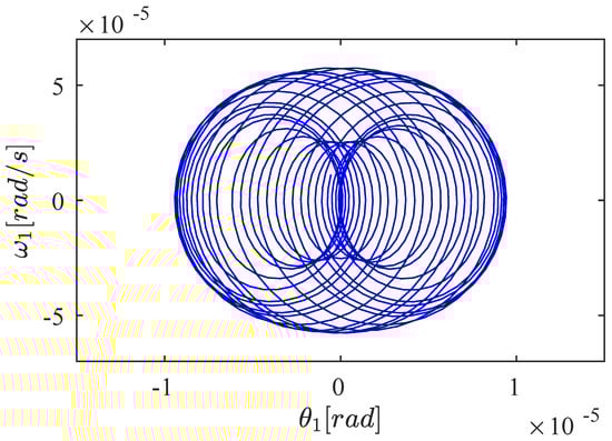
Figure 10. Phase diagram ${\omega }_1$ vs ${\theta }_1$ with initial conditions ${({\theta }_1,{\theta }_2,{\omega }_1,{\omega }_2)}_0=(0,0.01,0,0)$. The motion depends on two frequencies, $f_1\cong 1.4$ 1/s and $f_2\cong 0.55$ 1/s. The simulation duration is 20 s.

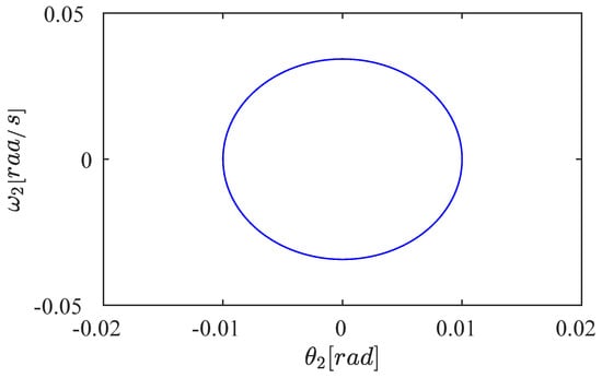
Figure 11. Phase diagram ${\omega }_2$ vs ${\theta }_2$ with initial conditions ${({\theta }_1,{\theta }_2,{\omega }_1,{\omega }_2)}_0=(0,0.01,0,0)$. The motion depends on only one frequency, $f_2\cong 0.55$ 1/s. The simulation duration is 20 s.

The second example corresponds to the initial conditions ${({\theta }_1,{\theta }_2,{\omega }_1,{\omega }_2)}_0=(0.01,0,0,0)$. We obtain $A_{11}=A_{12}=0.0049999499392039395$ and $A_{13}=A_{14}=5.0060796060752083\times {10}^{-8}$. The comparison between the analytical and numerical results is shown in Figure 12 and Figure 13. The differences between analytical and numerical results can be evaluated using the absolute value of the highest difference $M_d$, the mean error $E_m$, and the standard deviation $\sigma$. For ${\theta }_1$, we calculate $M_d=1.0897\times {10}^{-5}$, $E_m=-6.1962\times {10}^{-8}$, and $\sigma =2.7258\times {10}^{-18}$, and for ${\theta }_2$, we obtain $M_d=2.2916\times {10}^{-7}$, $E_m=1.3222\times {10}^{-9}$, and $\sigma =7.9839\times {10}^{-21}$. In both tests, the numerical results accurately verify the theoretical predictions.

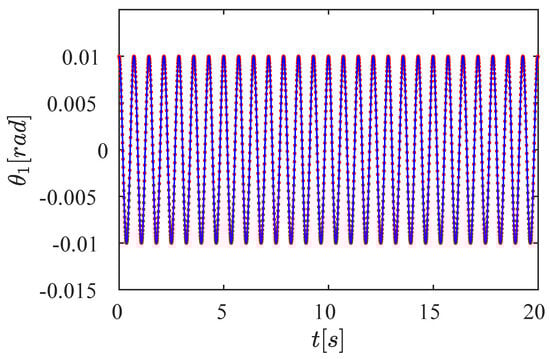
Figure 12. Analytical and numerical result for ${\theta }_1$ with initial conditions ${({\theta }_1,{\theta }_2,{\omega }_1,{\omega }_2)}_0=(0.01,0,0,0)$. The blue line represents the analytical results, and the red points are the numerical data. Highest difference $M_d=1.0897\times {10}^{-5}$, mean error $E_m=-6.1962\times {10}^{-8}$, and standard deviation $\sigma =2.7258\times {10}^{-18}$. The numerical results show a high accuracy with the theoretical data. For ${\theta }_1$, only one frequency $f_{+}\cong 1.4$ 1/s is present. The simulation duration is 20 s.

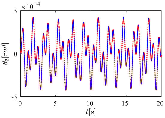
Figure 13. Analytical and numerical result for ${\theta }_2$ with initial conditions ${({\theta }_1,{\theta }_2,{\omega }_1,{\omega }_2)}_0=(0.01,0,0,0)$. The blue line represents the analytical results, and the red points are the numerical data. The highest difference is $M_d=2.2912\times {10}^{-7}$, the mean error is $E_m=1.3222\times {10}^{-9}$, and the standard deviation is $\sigma =7.9839\times {10}^{-21}$. The numerical data demonstrate high accuracy in comparison to the analytical results. The motion of ${\theta }_2$ shows two frequencies $f_{+}\cong 1.4$ 1/s and $f_{-}\cong 0.55$ 1/s. The simulation duration is 20 s.

Note that $|A_{11}|=|A_{12}|\gg |A_{13}|=|A_{14}|$ implies that ${\theta }_1$ depends only on ${\omega }_{+}$. In addition to this, the products $|{\displaystyle \frac{k_4-k_1{\omega }_{+}^2}{k_2{\omega }_{+}^2}}{A}_{11}|$ and $|{\displaystyle \frac{k_4-k_1{\omega }_{+}^2}{k_2{\omega }_{+}^2}}{A}_{12}|$ have the same order as $|{\displaystyle \frac{k_4-k_1{\omega }_{-}^2}{k_2{\omega }_{-}^2}}{A}_{13}|$ and $|{\displaystyle \frac{k_4-k_1{\omega }_{-}^2}{k_2{\omega }_{-}^2}}{A}_{14}|$, which implies that the evolution of ${\theta }_2$ depends on both angular velocities ${\omega }_{+}$ and ${\omega }_{-}$.

Using small perturbations allows us to utilize the linearized system given by Equations (56) and (57) instead of the general system (39) and (40). This means neglecting the following terms in Equation (39): $2k_{2}sin({\theta }_1+{\theta }_2)\left(-(\dot{{\theta }_1}+\dot{{\theta }_2})\dot{{\theta }_1}+\dot{{\theta }_1}\dot{{\theta }_2}\right)$, and the following terms in Equation (40): $2k_{2}sin({\theta }_1+{\theta }_2)\left(-(\dot{{\theta }_1}+\dot{{\theta }_2})\dot{{\theta }_1}+\dot{{\theta }_1}\dot{{\theta }_2}\right)$. In our analysis, we have considered that the small perturbations approximation is valid if the sum of the neglected terms does not exceed $5\%$ of the sum of the terms in the linearized equations:

$$2k_{2}sin({\theta }_1+{\theta }_2)\left(-(\dot{{\theta }_1}+\dot{{\theta }_2})\dot{{\theta }_1}+\dot{{\theta }_1}\dot{{\theta }_2}\right)<0.05\left(2k_1\ddot{{\theta }_1}+2k_2\ddot{{\theta }_2}+mg{l}_1\left(2a_1-{\displaystyle \frac{1}{2}}\right){\theta }_1\right)$$

(68)

$$2k_{2}sin({\theta }_1+{\theta }_2)\left(-(\dot{{\theta }_1}+\dot{{\theta }_2})\dot{{\theta }_1}+\dot{{\theta }_1}\dot{{\theta }_2}\right)<0.05\left(2k_3\ddot{{\theta }_2}+2k_2\ddot{{\theta }_1}+mg{l}_2{a}_2{\theta }_2\right).$$

(69)

This evaluation depends on the imposed initial condition because the system’s evolution depends on it. Therefore, when ${\theta }_{1_0}$ is varied, leaving ${\theta }_{2_0}=0$, we obtain a limiting energy $E_{l_1}=0.2197657829$ J, which corresponds to an initial ${\theta }_{1_0}=0.031416$. If the initial ${\theta }_{2_0}$ is varied while maintaining ${\theta }_{1_0}=0$, we obtain $E_{l_2}=0.22042185$ J and ${\theta }_{2_0}=1.2566$. Thus, the equilibrium energy for ${\theta }_{1_0}=0$ and ${\theta }_{2_0}=0$ is $E_1=0.219744$ J, and the energy limit for small perturbations is $E_{l_1}=E_{l_2}=0.2197657829$ J.

We highlight that the numerical data were calculated solving the system (41)–(44), and the analytical results were obtained using the linearized system (39) and (40). Thus, the ability to evaluate analytical results for low-energy motions enables us to validate the behavior of the numerical integrator scheme and ensure that the developed software is free of errors.

In [8], a study of small perturbations in a double pendulum with distributed mass is presented. The authors identify a system similar to Equations (56) and (57) and calculate two normal frequencies. However, they do not provide a detailed analysis of how the system’s dynamics depend on the initial conditions.

6. Conclusions and Outlook

In this study, we examined the motions of small perturbations in a swinging stick pendulum and investigated how the dynamics of the system are affected by the initial shape of these small perturbations. To describe the equations of motion for this intricate system, we used Lagrangian mechanics. The equilibrium configurations were determined by minimizing the potential energy, which imposed constraints on the system parameters. We deduced, using the Hessian matrix, the necessary conditions to have only one stable equilibrium point in $({\theta }_1,{\theta }_2)=(0,0)$, where subscripts 1 and 2 refer to the first and second sticks of the device, respectively.

Starting from the Euler–Lagrange equations, we derived a four-dimensional autonomous dynamical system characterized by two angular positions and two angular velocities, denoted as $({\theta }_1,{\theta }_2,{\omega }_1,{\omega }_2)$. The motion near the stable point $({\theta }_1,{\theta }_2,{\omega }_1,{\omega }_2)=(0,0,0,0)$ was analyzed both numerically and analytically. Numerical solutions were obtained using the Bulirsch–Stoer method, while analytical closed forms were gained through a normal mode analysis. To complement these approaches, we performed a fast Fourier transform (FFT) analysis and constructed Poincaré maps to study the system’s dynamics. Four different sets of initial conditions—small perturbations—were examined.

When the small initial perturbation was applied to ${\theta }_1$ or ${\omega }_1$ (i.e., the first stick), its motion was governed by a single frequency, whereas the second stick exhibited dynamics involving two incommensurate frequencies. However, the first stick showed a much greater amplitude and angular velocity than the second stick. Conversely, when the small initial disturbances affected only ${\theta }_2$ or ${\omega }_2$ (i.e., the second stick), the roles were reversed: the second stick followed a single-frequency motion, while the first was influenced by two incommensurate frequencies. In addition, in this case, the second rod moved with greater amplitude and angular velocity than the first rod. When motions depend on one frequency, they are periodic. However, if the motions depend on two frequencies, they are quasiperiodic.

Finally, we emphasize that the agreement between the numerical, analytical, and fast Fourier transform results was remarkably high across all tests. This strong consistency lays a solid foundation for the second part of this study, which will address the response of the system to general (non-small) initial disturbances.

References

- Schuster, H.; Just, W. Deterministic Chaos; Wiley VCH: Mörlenbach, Germany, 2005. [Google Scholar]
- Lichtenberg, A.; Liebermann, M. Regular and Stochastic Motion; Springer: Berlin/Heidelberg, Germany; Springer: New York, NY, USA, 1983. [Google Scholar]
- Richter, P.; Scholz, H. Chaos in Classical Mechanics: The Double Pendulum. In Stochastic Phenomena and Chaotic Behaviour in Complex Systems, Proceedings of the Fourth Meeting of the UNESCO Working Group on Systems Analysis Flattnitz, Kärnten, Austria, 6–10 June 1983; Springer: Berlin/Heidelberg, Germany, 1984. [Google Scholar]
- Moshe, G. The Chaotic Pendulum; World Scientific Publishing Co. Pte Ltd.: Singapore, 2010. [Google Scholar]
- Calvao, A.; Penna, T. The double pendulum: A numerical study. Eur. J. Phys. 2015, 36, 045018. [Google Scholar] [CrossRef]
- Shinbrot, T.; Grebogi, C.; Wisdom, J.; Yorks, H. Chaos in a double pendulum. Am. J. Phys. 1982, 60, 491–499. [Google Scholar] [CrossRef]
- Levien, R.; Tan, S. Double pendulum: An experiment in chaos. Am. J. Phys. 1993, 61, 1038. [Google Scholar] [CrossRef]
- Rafat, M.; Wheatland, M.; Bedding, T. Dynamics of a double pendulum with distributed mass. J. Phys. 2009, 77, 216. [Google Scholar] [CrossRef]
- Stachowiak, T.; Okada, T. A numerical analysis of chaos in the double pendulum. Chaos Solitons Fractals 2006, 29, 417–422. [Google Scholar] [CrossRef]
- Korsch, H.; Jodl, H.; Hartmann, T. Chaos: A Program Collection for the PC; Springer: Berlin, Germany, 2008. [Google Scholar]
- Li, Y.; Qiu, J.; Lan, T.; Song, H. Multi-directional extremely-low-frequency electromagnetic ocean wave energy harvester based on improved double pendulum structure. AIP Adv. 2023, 13, 015033. [Google Scholar] [CrossRef]
- Goldstein, H.; Poole, C.; Safko, J. Classical Mechanics; Addison-Wesley: New York, NY, USA, 2002. [Google Scholar]
- Thompson, J.; Stewart, H. Nonlinear Dynamics and Chaos; John Wiley & Sons Ltd.: Chichester, UK, 1986. [Google Scholar]
- Spivak, M. Calculus on Manifolds; Addison-Wesley Publishing Company: Boston, MA, USA, 1965. [Google Scholar]
- Boas, M.L. Mathematical Methods in Physical Sciences, 3rd ed.; John Wiley & Sons Ltd.: New York, NY, USA, 2006. [Google Scholar]
- Stoer, J.; Bulirsch, R. Introduction to Numerical Analysis, 2nd ed.; Springer: New York, NY, USA, 1993. [Google Scholar]
- Deuflhard, P. Recent progress in extrapolation methods for ordinary differential equations. SIAM Rev. 1985, 27, 505–535. [Google Scholar] [CrossRef]
- Douglas Gregory, R. Classical Mechanics; Cambridge University Press: Cambridge, UK, 2006. [Google Scholar]
- Nayfeh, A.; Balachandran, B. Applied Nonlinear Dynamics; Wiley: New York, NY, USA, 1995. [Google Scholar]
- Elaskar, S.; del Rio, E. New Advances on Chaotic Intermittency and Applications; Springer: Cham, Switzerland, 2017. [Google Scholar]
- Available online: https://mathworks.com (accessed on 5 August 2025).
- Gaberson, H. A comprehensive windows tutorial. Sound Vib. 2006, 40, 14–23. [Google Scholar]
- Thornton, S.; Marion, J. Classical Dynamics of Particles and Systems, 5th ed.; Brooks/Cole-Thomson Learning: Boston, MA, USA, 2004. [Google Scholar]
Disclaimer/Publisher’s Note: The statements, opinions and data contained in all publications are solely those of the individual author(s) and contributor(s) and not of MDPI and/or the editor(s). MDPI and/or the editor(s) disclaim responsibility for any injury to people or property resulting from any ideas, methods, instructions or products referred to in the content. |
© 2025 by the authors. Licensee MDPI, Basel, Switzerland. This article is an open access article distributed under the terms and conditions of the Creative Commons Attribution (CC BY) license (https://creativecommons.org/licenses/by/4.0/).