S-ResGCN-I: A Symmetry-Enhanced Residual Graph Convolutional Network for MRI-Based Brain Tumor Classification

Abstract

Early and accurate detection of brain tumors is critical for MRI-based diagnosis. Conventional convolutional neural networks often struggle to capture fine-grained details, small or boundary-ambiguous lesions, and hemispheric symmetry patterns. To address these limitations, we propose S-ResGCN, a symmetry-aware framework integrating hierarchical feature extraction, attention mechanisms, and graph-based classification. S-ResGCN employs a ResNet50 backbone to extract multi-level features, with Convolutional Block Attention Modules applied to intermediate and deep layers to enhance key information and discriminative features. Furthermore, we introduce a novel self-paired regularization to enforce feature consistency between original and horizontally flipped images, improving sensitivity to bilateral symmetric structures. Extracted features are converted into nodes and modeled as a small graph, and a graph convolutional network captures inter-node relationships to generate symmetry-aware predictions. Evaluation on three publicly available brain tumor MRI datasets demonstrates that S-ResGCN achieves average accuracies of 99.83%, 99.37% and 99.26% ± 0.16, with consistently high precision, recall, and F1-scores. These results indicate that S-ResGCN effectively captures fine-grained and symmetric tumor characteristics often overlooked by conventional models, providing a robust and efficient tool for automated, graph convolutional network.

1. Introduction

Brain tumors are among the most common and aggressive malignancies of the central nervous system, typically arising from the abnormal proliferation of glial or meningeal cells. They pose a severe threat to neurological function and patient survival. Epidemiological studies indicate that brain tumors rank among the leading causes of mortality and disability in neurological disorders, particularly when lesions occur in critical brain regions where they can profoundly impair speech, motor, and cognitive functions. In addition to their heterogeneous and irregular morphologies, brain tumors often exhibit locally symmetric growth patterns, which complicates accurate identification and precise boundary delineation. Consequently, early detection and timely intervention are essential for improving survival rates, delaying disease progression, and optimizing patient outcomes. Prompt tumor identification not only reduces surgical risks but also prevents irreversible neurological damage.

Magnetic resonance imaging (MRI) [1], with its superior soft-tissue contrast, non-ionizing nature, and multi-sequence imaging capability, has become an indispensable modality for clinical brain tumor diagnosis. MRI enables clear visualization of abnormal brain structures, providing reliable evidence for tumor detection, localization, and grading. However, the interpretation of MRI scans is highly dependent on radiologists’ expertise and subjective judgment. This dependence can prolong diagnostic time and introduce variability due to differences in clinical experience or visual fatigue, ultimately reducing diagnostic consistency and accuracy. To address these challenges, traditional computer-aided diagnosis (CAD) [2] methods have been extensively applied to brain MRI analysis. Such approaches rely on handcrafted feature extraction—commonly including texture descriptors (e.g., gray-level co-occurrence matrices, local binary patterns), shape features, and statistical measures—followed by classification using machine learning algorithms such as support vector machines (SVM) [3], random forests (RF) [4], or k-nearest neighbors (KNN) [5]. Although these methods achieved early success, their labor-intensive feature engineering, subjectivity, and limited generalization ability hinder their effectiveness for the complex, diverse, and locally symmetric morphological characteristics of brain tumors.

In recent years, deep learning has emerged as the dominant paradigm for medical image analysis, with convolutional neural networks (CNNs) [6] demonstrating remarkable performance in brain tumor classification tasks. For example, Musa et al. [7] constructed a ResNet50-based detection model that effectively assisted radiologists in identifying abnormal regions and improving diagnostic accuracy. Ahmed et al. [8] proposed an optimized CNN architecture that significantly enhanced classification performance while maintaining manageable model complexity. Other studies have incorporated pretrained networks to improve generalization; Nizamli et al. [9] used a fixed-weight VGG-19 network to convert MRI images into high-level feature representations combined with an SVM classifier, achieving shorter training times without compromising accuracy. Similarly, Haq et al. [10] integrated CNNs with long short-term memory networks to capture both spatial and temporal information, further improving performance through data augmentation. However, these approaches often rely heavily on global features and fail to explicitly capture fine local details and symmetry-related structures, resulting in reduced sensitivity to small, blurred, or irregular lesions—critical for precise clinical diagnosis.

To design deep learning architectures that are robust and sensitive to local symmetry, insights from graph theory and complex network analysis can be particularly valuable. Previous studies—such as those by Wang et al. [11], Wang et al. [12,13] and Jiang et al. [14]—have systematically investigated the connectivity and diagnosability of locally twisted cubes, leaf-sort graphs, and maximally 4-restricted edge-connected graphs. Additionally, the connectivity and diagnosability of leaf-sort graphs were further explored in a separate study by Wang et al. [15]. The diagnosability of interconnection networks was discussed by Xiang et al. [16], and the connectivity of m-ary n-dimensional hypercubes was investigated in [17,18,19]. These studies highlight the importance of information-flow reliability, fault tolerance, and node-level symmetry in complex networks, providing a conceptual foundation for developing deep learning architectures capable of capturing local structural and symmetric patterns in brain MRI. Zarenia et al. [20] further combined data augmentation techniques with a hierarchical mul-ti-scale deformable attention module (MS-DAM) to effectively capture irregular and complex tumor patterns, thereby significantly enhancing the model’s classification performance.

Motivated by these considerations, we propose S-ResGCN, a symmetry-aware framework for brain tumor classification. Compared with conventional approaches, the main contributions of S-ResGCN are: (1) Using a ResNet50 backbone for hierarchical feature extraction, with Convolutional Block Attention Modules (CBAM) [21] applied to intermediate and deep layers to enhance key information and discriminative features. (2) Inspired by consistency regularization approaches [22], we introduce a novel self-paired regularization (SPR) loss, which enforces feature consistency between original and horizontally flipped images, improving sensitivity to bilateral structures. (3) Constructing node features via global average pooling and modeling inter-node relationships with a graph convolutional network (GCN) [23] head, enabling symmetry-aware predictions for robust detection of complex and symmetric lesions.

2. Materials and Methods

2.1. Dataset

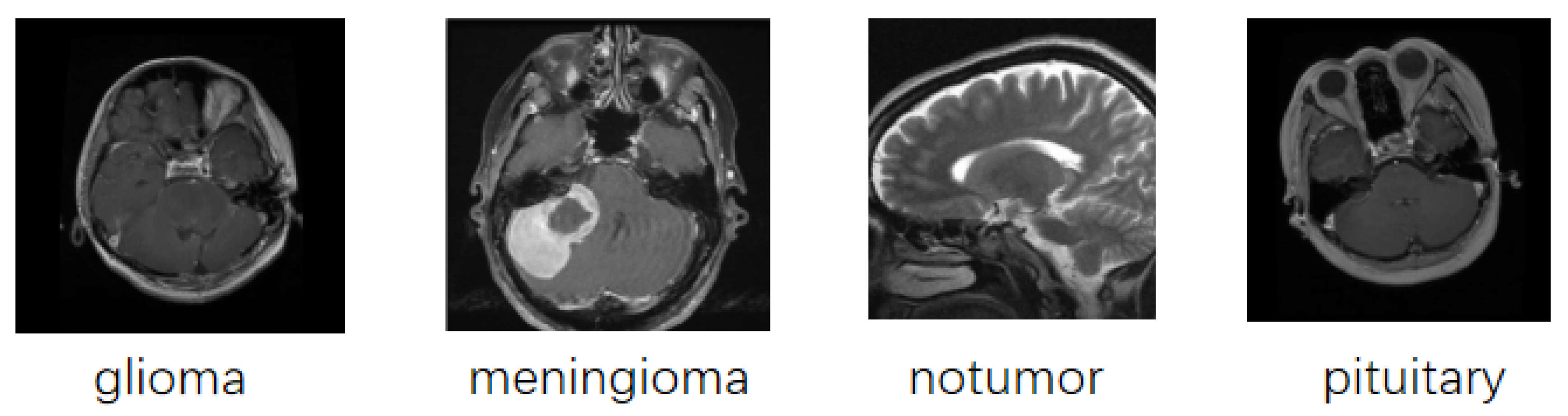
We retrospectively collected a total of 7023 MRI images from the Brain Tumor MRI Dataset [24] and 3264 MRI images from the Brain Tumor MRI Dataset [25]. As shown in Figure 1, both datasets encompass four tumor categories. Dataset I comprises 2000 images of No Tumor, 1757 images of Pituitary Tumor, 1621 images of Glioma, and 1645 images of Meningioma. Dataset II contains 500 images of No Tumor, 900 images of Pituitary Tumor, 926 images of Glioma, and 937 images of Meningioma. Dataset III was provided by the General Hospital and Nanfang Hospital of Tianjin Medical University and was publicly released online by Cheng, Jun et al. [26]. It contains a total of 3064 MRI images covering three types of brain tumors: 708 images of meningioma, 1426 images of glioma, and 930 images of pituitary tumors.These images cover a wide spectrum of tumor types and patient demographics and were carefully curated to ensure sufficient quality for subsequent analyses.

2.2. S-ResGCN Model

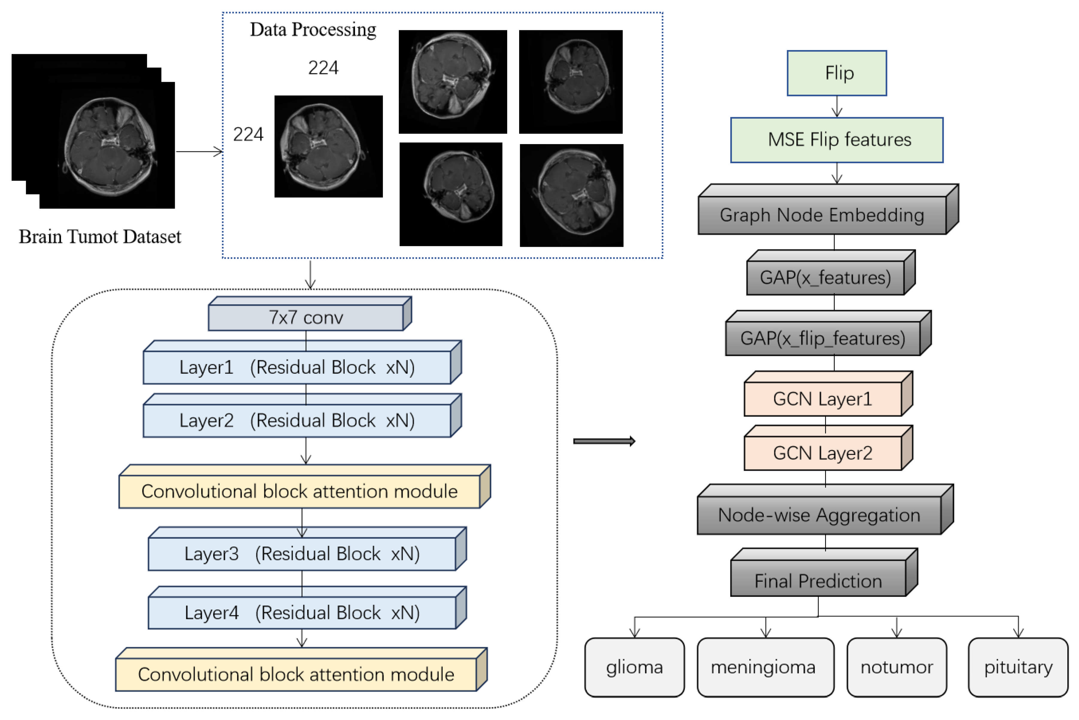
The S-ResGCN model, illustrated in Figure 2, utilizes a standard ResNet50 backbone to extract hierarchical feature representations from input MRI images, effectively capturing low-level textures and edge information. Convolutional Block Attention Modules (CBAMs) are integrated after the second and fourth residual blocks to enhance both channel-wise and spatial attention, emphasizing symmetric and discriminative features. Finally, a graph convolutional network (GCN) classification head is applied to the extracted features, incorporating information from both the original and horizontally flipped images to achieve symmetry-aware classification.

Initially, the input MRI images underwent systematic preprocessing and data augmentation to enhance model generalization and reinforce symmetry-aware feature learning. The augmentation pipeline included random rotations, flips, color jittering, and affine transformations. Specifically, each image was randomly rotated within $\pm {30}^{\circ }$, randomly flipped along both horizontal and vertical axes to preserve spatial symmetry, subjected to brightness and contrast adjustments for color jittering, and transformed via translation and scaling. For each original image, five augmented variants were generated, and all images were resized to a uniform dimension of $224\times 224$ pixels.

For an input image $X_{\mathrm{input}}$, local convolutional features are first extracted to generate a feature map $X\in {\mathbb{R}}^{C\times H\times W}$, where C denotes the number of channels, and H and W denote the height and width, respectively. The original $7\times 7$ convolution in the first layer (conv1) followed by batch normalization and ReLU activation, and a $3\times 3$ max-pooling layer produces an initial feature map:

$$X_1=MaxPool\left(ReLU\left(BN\left({Conv}_{7\times 7}\left(X_{\mathrm{input}}\right)\right)\right)\right).$$

(1)

where ${Conv}_{7\times 7}(·)$ represents a $7\times 7$ convolution operation, $BN(·)$ denotes batch normalization, $ReLU(·)$ is the rectified linear unit activation function, and $MaxPool(·)$ refers to a $3\times 3$ max-pooling operation.

The feature map $X_1$ is then propagated through the first residual block (layer1), generating:

$$X_2={Layer}_1\left(X_1\right).$$

(2)

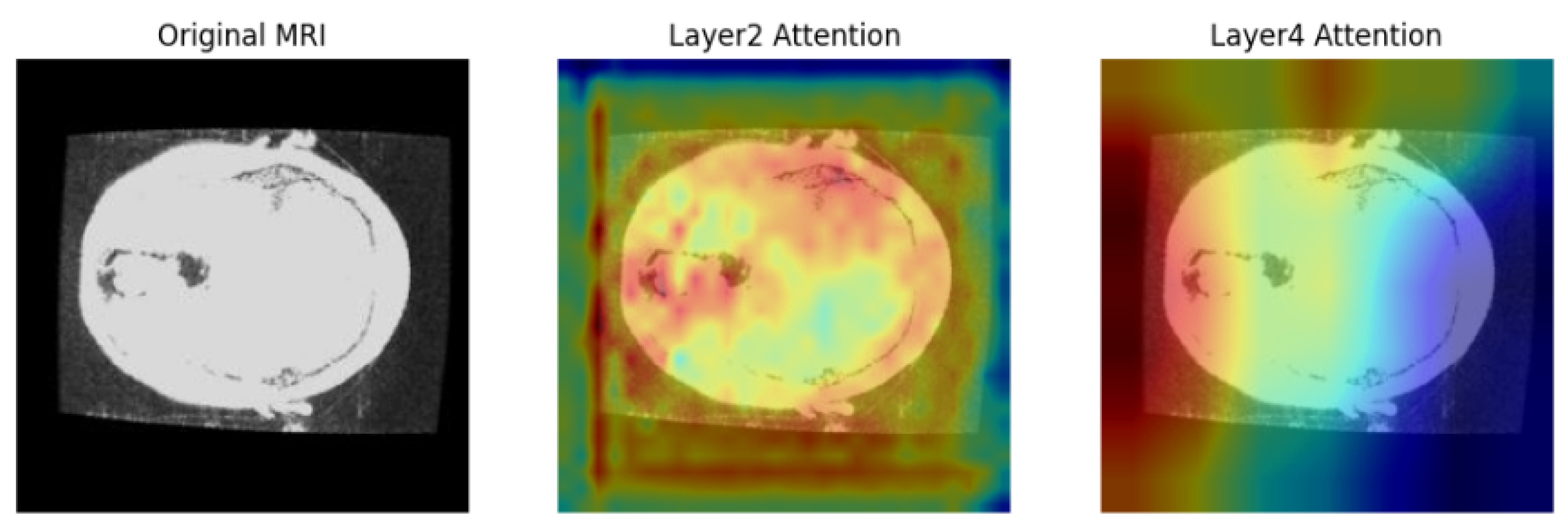
Next, as shown in Figure 3, the CBAM was integrated after the second and fourth residual blocks, while the first and third residual blocks were not selected. Features in the first residual block mainly capture low-level information such as edges and textures, with limited semantic content; applying attention at this stage may not significantly enhance discriminative capability. The third residual block, although containing more semantic information, has reduced spatial resolution, resulting in partial loss of local details, which limits the effectiveness of attention for refining boundaries and fine structures. After the second residual block, the feature maps already contain some semantic information while retaining rich spatial details. At this stage, CBAM applies channel attention and spatial attention to recalibrate the feature maps: channel attention adaptively adjusts the importance of each feature channel, enabling the network to focus on channels carrying discriminative information, while spatial attention highlights key regions and suppresses irrelevant background. This mechanism enhances sensitivity to local details, facilitating precise tumor boundary detection and the capture of left–right symmetry features. After the fourth residual block, the feature maps become more abstract and semantically rich. At this stage, the CBAM primarily strengthens global discriminative capability: channel attention emphasizes feature channels that are globally informative, and spatial attention highlights critical regions across the entire image, helping the model more effectively differentiate between tumor types and healthy tissue. By applying attention at different network depths, the CBAM balances local detail and global semantic understanding, enabling the model to capture fine-grained boundary information while comprehending overall structural patterns, thereby improving classification performance and generalization.

The second residual block is applied, followed by the CBAM to emphasize symmetric and discriminative features:

$$X_3={CBAM}_2\left({Layer}_1\left(X_2\right)\right),$$

(3)

where ${Layer}_k$ denotes the k-th residual layer, and ${CBAM}_k$ represents the attention module in that stage.

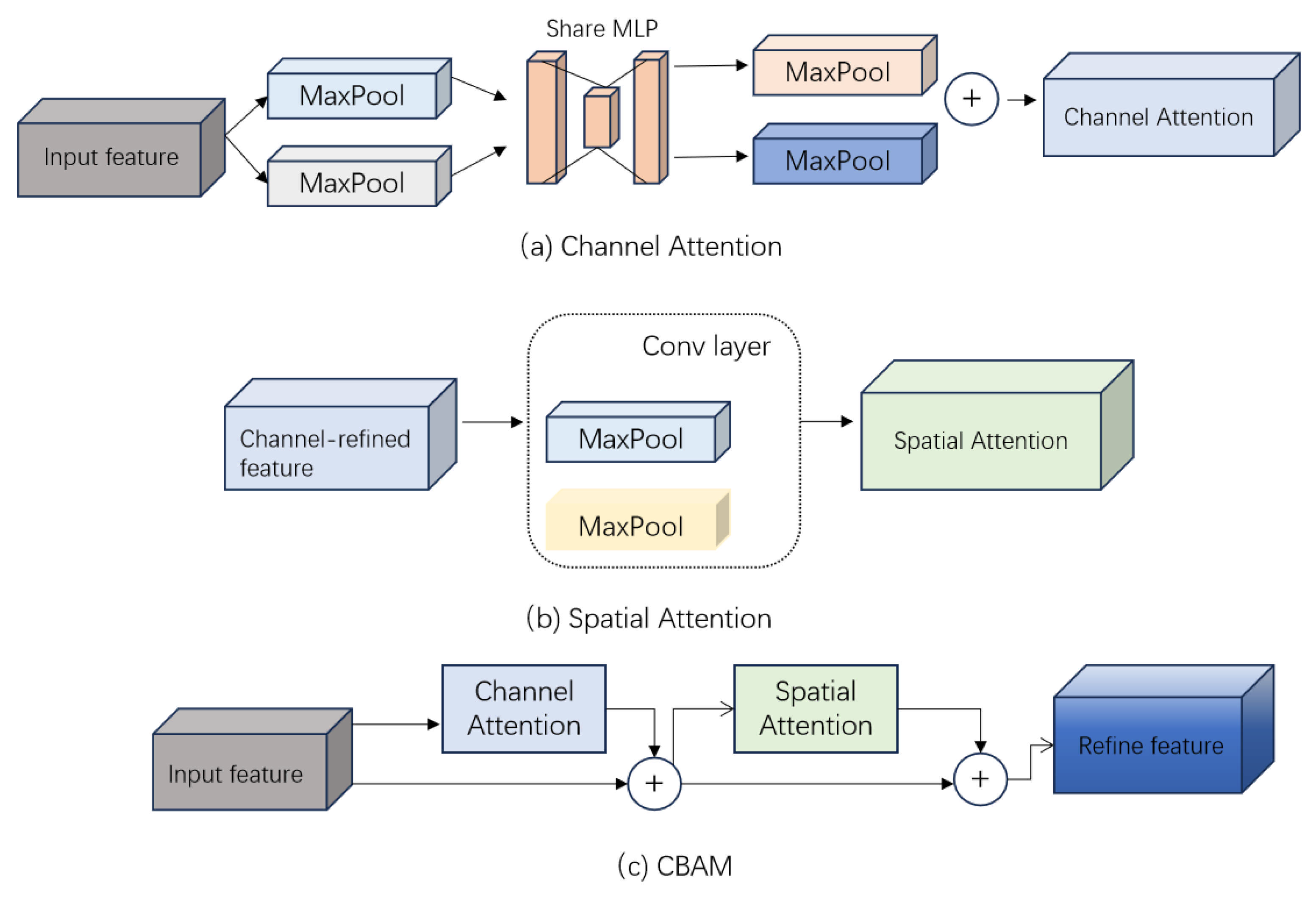
The CBAM sequentially applies channel and spatial attention to emphasize symmetric and discriminative features. As shown in Figure 4, the channel attention mechanism refines the input feature by aggregating spatial information through global average pooling and max pooling, followed by a shared multi-layer perceptron to generate a channel attention map. The channel attention is computed as:

$$A_{\mathrm{channel}}=\sigma \left(W_{2}ReLU(W_1·GAP\left(X_2\right))\right),$$

(4)

where $GAP(·)$ represents global average pooling, $W_1$ and $W_2$ are learnable weight matrices of the shared multi-layer perceptron, $\sigma (·)$ is the sigmoid activation function, and $A_{\mathrm{channel}}$ is the resulting channel attention map.

Spatial attention is computed as:

$$A_{\mathrm{spatial}}=\sigma \left(Conv\left([GAP\left(X_2\right),MaxPool\left(X_2\right)]\right)\right),$$

(5)

The CBAM-enhanced feature map is then obtained by:

$${\displaystyle X_3^{\prime }}=X_3·A_{\mathrm{channel}}·A_{\mathrm{spatial}}+X_3,$$

(6)

where · denotes element-wise multiplication, and ${\displaystyle X_3^{\prime }}$ is the CBAM-enhanced feature map.

Similarly, the feature map is propagated through layer3:

$$X_4={Layer}_1\left({\displaystyle X_3^{\prime }}\right),$$

(7)

$$X_5={CBAM}_4\left({Layer}_1\left(X_4\right)\right).$$

(8)

To reinforce symmetry-aware feature learning, each input image was horizontally flipped to obtain $X_{\mathrm{flip}}$, and its feature map was extracted through the backbone network:

$$X_{\mathrm{flip}\_\mathrm{features}}=Backbone\left(X_{\mathrm{flip}}\right)$$

(9)

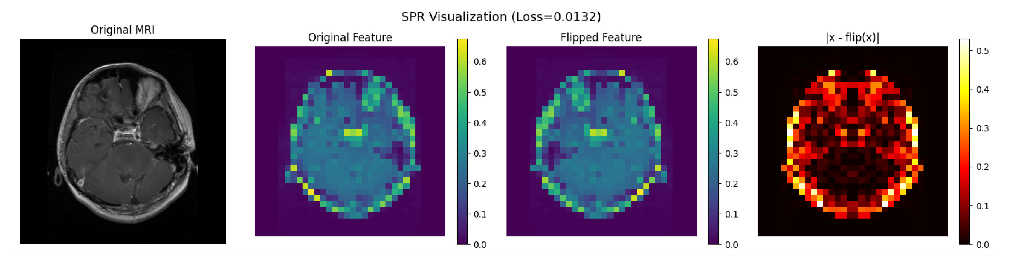
The self-paired regularization (SPR) loss enforces symmetry consistency between the original and flipped features, as illustrated in Figure 5. Encouraging the network to be sensitive to symmetric structures commonly observed in brain tumors. To prevent redundancy or potential data leakage during training, explicit controls are applied: flips for data augmentation are randomly applied to input images to improve model generalization, whereas flips for SPR are performed at the feature-map level to compute a symmetry loss between original and mirrored features. These operations occur at different levels, avoiding direct reuse of the same data. Furthermore, the SPR loss is applied only during training for regularization and does not introduce information from the validation or test sets; mirrored features participate only within the current mini-batch, ensuring no leakage of label information. The SPR loss is computed as:

$$L_{\mathrm{SPR}}={\displaystyle \frac{1}{B}}{\displaystyle \sum _{b=1}^B}{\displaystyle {∥{\displaystyle X_5^{\left(b\right)}}-{\displaystyle X_{\mathrm{flip}\_\mathrm{features}}^{\left(b\right)}}∥}_2^2}$$

(10)

where B is the batch size, ${\displaystyle X_5^{\left(b\right)}}$ denotes the backbone feature map of the b-th original image (after CBAM), and ${\displaystyle X_{\mathrm{flip}\_\mathrm{features}}^{\left(b\right)}}$ denotes the corresponding flipped feature map. The squared L2 norm ${\displaystyle {∥·∥}_2^2}$ measures the discrepancy between symmetric feature representations.

Finally, the feature maps of the original and flipped images are aggregated via Global Average Pooling:

$$Nod{e}_0=GAP\left(X_5\right),Nod{e}_1=GAP\left(X_{\mathrm{flip}\_\mathrm{features}}\right)$$

(11)

Graph nodes are constructed as:

$$X_{\mathrm{nodes}}=[Nod{e}_0,Nod{e}_1]$$

(12)

The GCN processes node features to produce node-level predictions:

$$H_1=GCNLaye{r}_1\left(X_{\mathrm{nodes}}\right),H_2=GCNLaye{r}_2\left(H_1\right)$$

(13)

The final prediction aggregates the outputs of original and flipped nodes:

$$\widehat{y}=softmax\left(\frac{1}{2}\left(H_2[:,0,:]+H_2[:,1,:]\right)\right)$$

(14)

where $Nod{e}_0$ and $Nod{e}_1$ denote the global average pooled feature vectors of the original and horizontally flipped images, respectively. $X_{\mathrm{nodes}}$ is the resulting node matrix, and $H_2$ is the intermediate node embeddings generated by the first and second GCN layers. $[:,0,:]$ and $[:,1,:]$ denote the feature vectors corresponding to the original and horizontally flipped nodes, respectively. Here, “:’’ indicates all elements along the batch or feature dimension, 0 and 1 select the first (original) and second (flipped) nodes, and the final $softmax$ converts the averaged node embeddings into a class probability vector $\widehat{y}$.

2.3. Experiment

In this study, Datasets I and II were partitioned into training and test sets at a 4:1 ratio to ensure sufficient diversity for model training. Dataset III was further evaluated using five-fold cross-validation, whereby the dataset was randomly divided into five equal subsets. In each fold, four subsets were used for training and the remaining subset for validation. This procedure was repeated five times, and the average performance across all folds was computed to comprehensively assess the model’s robustness and generalization capability.

We implemented an enhanced SymmetryResNet50 architecture (see

Table 1. SymmetryResNet50GCN Network Architecture and Output Sizes.

Stage/Layer	Output Size	Notes
Input	[B, 3, 224, 224]	RGB MRI image
conv1 + bn + relu	[B, 64, 112, 112]	7 × 7 convolution, stride 2
maxpool	[B, 64, 56, 56]	3 × 3 max pooling, stride 2
layer1	[B, 256, 56, 56]	3 × Bottleneck blocks (each block: 3 conv layers)
layer2 → CBAM2	[B, 512, 28, 28]	4 × Bottleneck blocks, CBAM applied after layer2
layer3	[B, 1024, 14, 14]	6 × Bottleneck blocks
layer4 → CBAM4	[B, 2048, 7, 7]	3 × Bottleneck blocks, CBAM applied after layer4
AdaptiveAvgPool → Flatten	[B, 2048, 1, 1] → [B, 2048]	Pool × and flipped separately
GCN input → output	[B, 2, 2048] → [B, num_classes]	2 GCN layers: 2048→256→n

) based on the PyTorch version 2.7.1 with CUDA 11.8 support deep learning framework, integrating multiple collaborative modules to strengthen feature representation and enforce structural symmetry constraints. All training and validation were conducted on a local workstation equipped with an NVIDIA GeForce RTX 3070 GPU (8 GB VRAM) under a CUDA 11.3 environment. The SymmetryResNet50GCN model contains approximately 25.5 million trainable parameters, including the ResNet50 backbone, CBAMs, and the GCN head. Self-Paired Regularization (SPR) imposes a mean-squared-error-based constraint between the original and horizontally flipped feature maps, with a regularization coefficient of $\lambda =0.05$. This regularization is applied only during training and does not affect validation or testing. The total loss is defined as the weighted sum of the cross-entropy loss and the SPR loss. Optimization is performed using AdamW with an initial learning rate of $5\times {10}^{-5}$ and a weight decay of $1\times {10}^{-4}$, combined with a cosine-annealing learning rate scheduler over 200 epochs. The batch size is set to 16. Peak GPU memory usage during training is approximately 6–8 GB, while inference requires roughly 2–3 GB of GPU memory.

Model performance was systematically evaluated using four standard metrics: Accuracy, Precision, Recall, and F1-score. Accuracy quantifies the overall classification correctness and is defined as:

$$\mathrm{Accuracy}={\displaystyle \frac{TP+TN}{TP+TN+FP+FN}}$$

(15)

where $TP$ denotes the number of true positives, $TN$ the number of true negatives, $FP$ the number of false positives, and $FN$ the number of false negatives.

Precision measures the proportion of correctly predicted positive samples for a given class:

$$\mathrm{Precision}={\displaystyle \frac{TP}{TP+FP}}$$

(16)

Recall evaluates the model’s ability to identify actual positive samples:

$$\mathrm{Recall}={\displaystyle \frac{TP}{TP+FN}}$$

(17)

The F1-Score provides a harmonic mean of Precision and Recall, balancing the trade-off between them:

$$\mathrm{F}1\mathrm{Score}={\displaystyle \frac{2\times (\mathrm{Precision}\times \mathrm{Recall})}{\mathrm{Precision}+\mathrm{Recall}}}$$

(18)

These metrics collectively provide a multi-dimensional assessment of the model’s classification performance across different tumor categories.

3. Results

3.1. Overall Performance

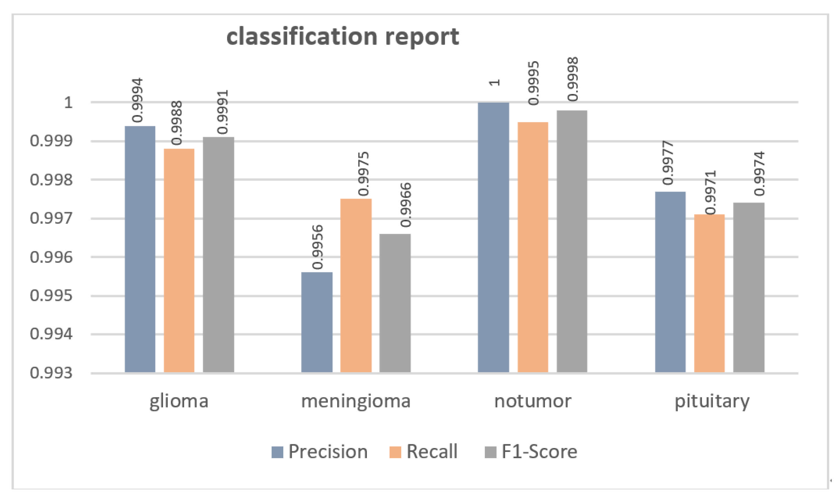
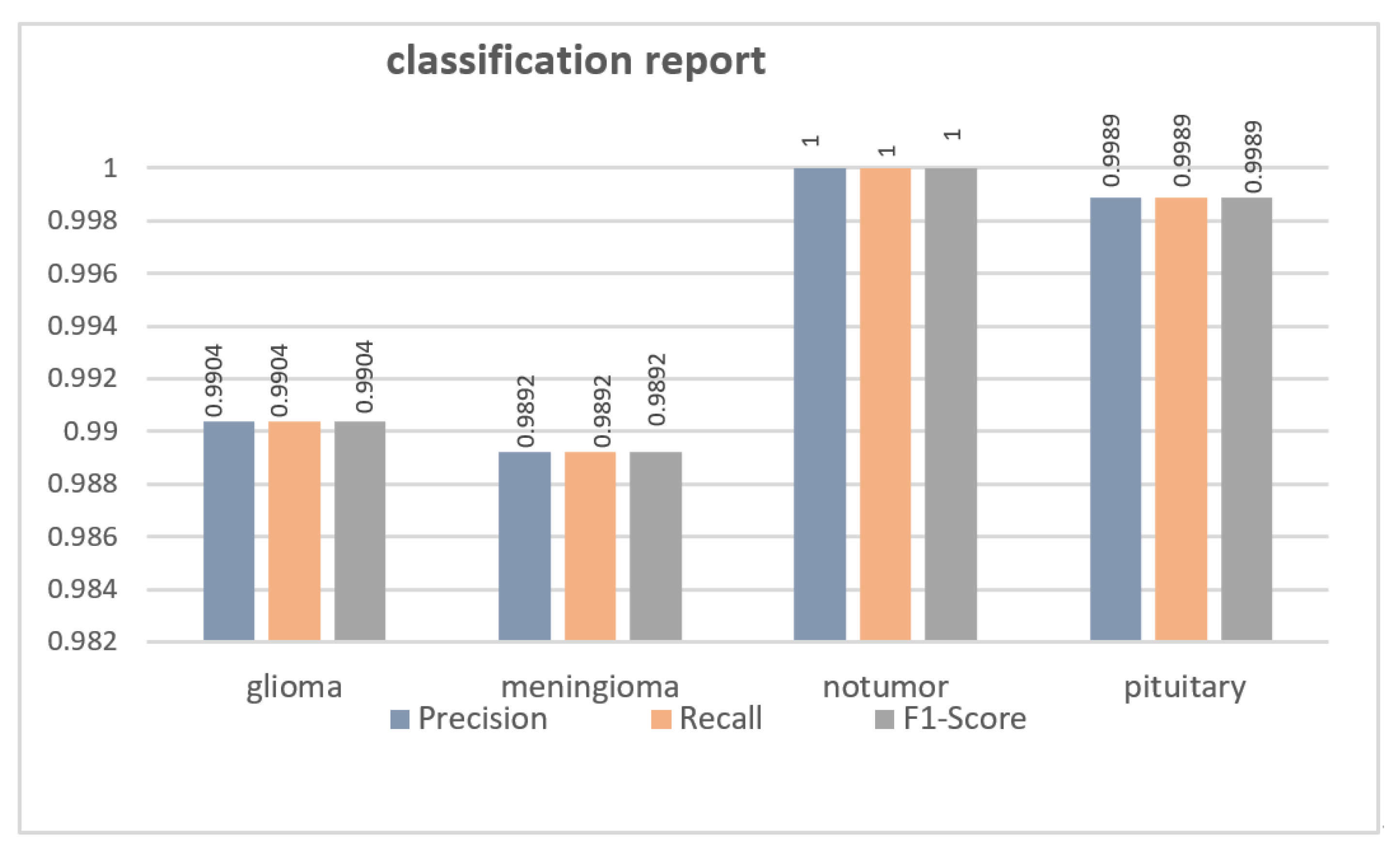
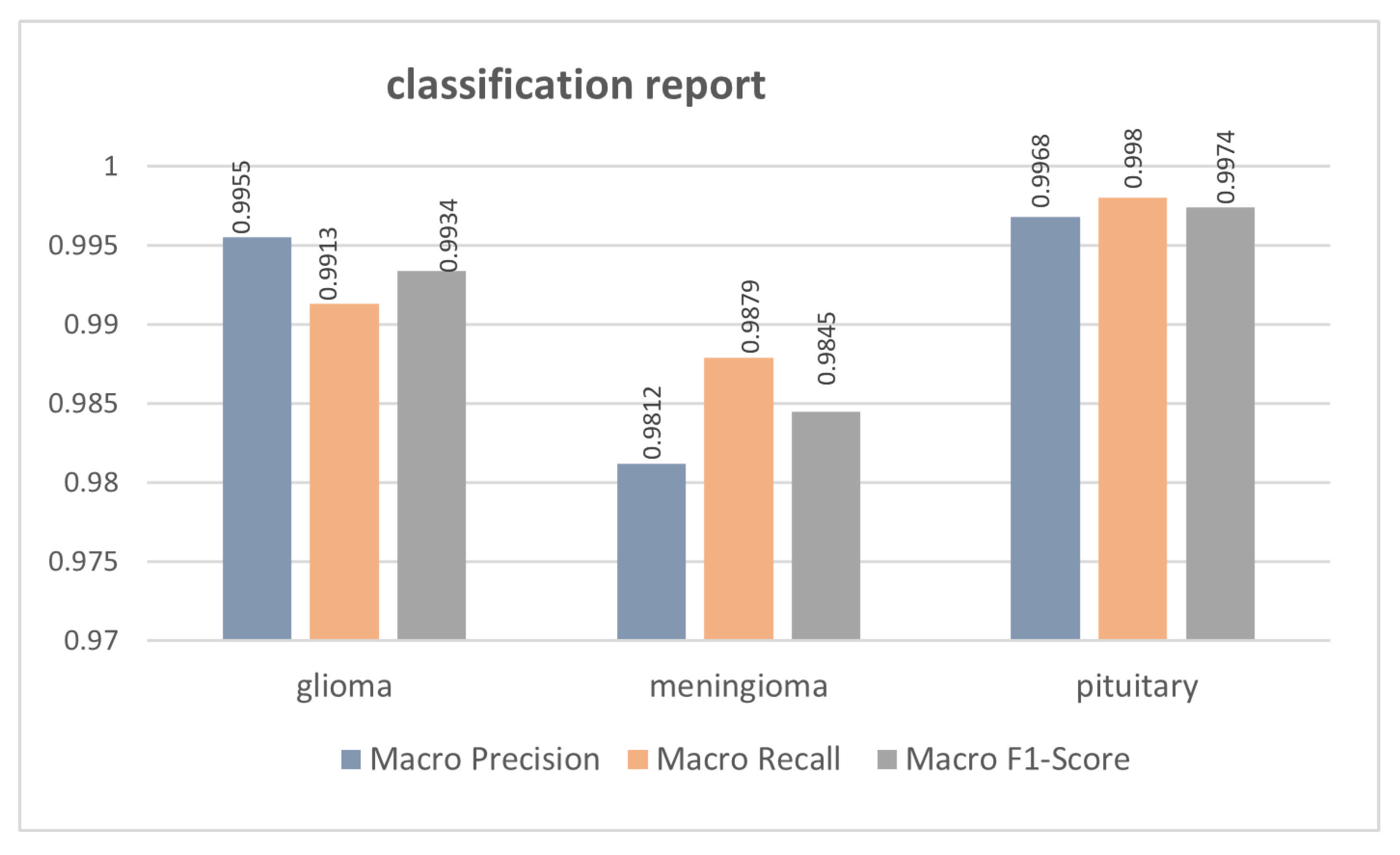
As shown in Figure 6 and Figure 7, the proposed S-ResGCN model exhibits outstanding performance on the four-class brain tumor classification task across both Dataset I and Dataset II. For all categories—including meningioma, glioma, no tumor, and pituitary—the model achieved Precision, Recall, and F1-Score values exceeding 98%, with the no tumor category in Dataset II reaching 100%, demonstrating exceptional robustness and highly consistent discriminative capability. In addition, as shown in Figure 8, the five-fold cross-validation results on Dataset III further demonstrate the stability and generalization capability of the proposed S-ResGCN model with minimal variation across folds, indicating highly consistent performance. All tumor categories—including glioma, meningioma, and pituitary—exhibited high precision, recall, and F1-scores, reflecting the model’s balanced discrimination across different classes.

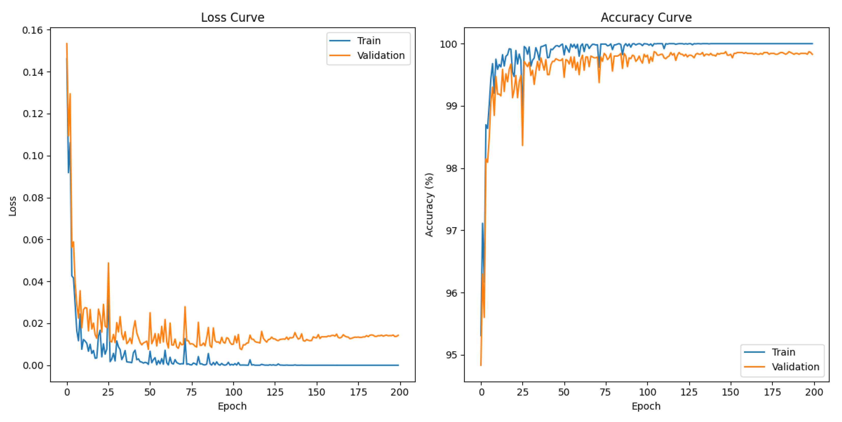
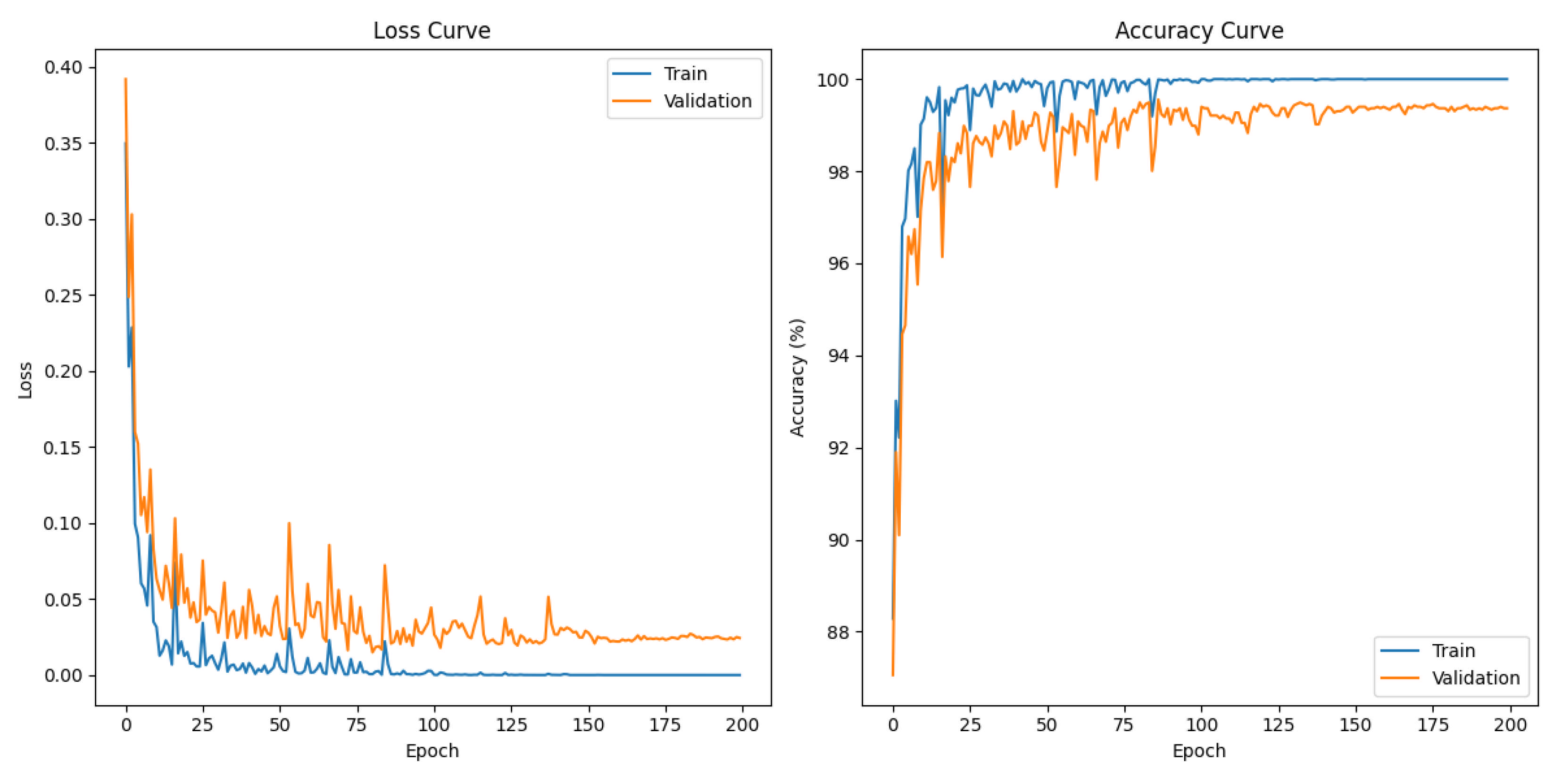
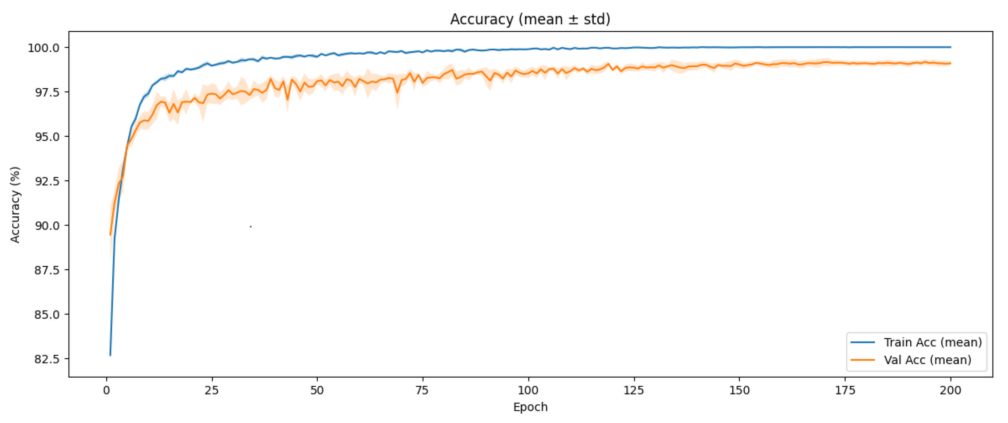
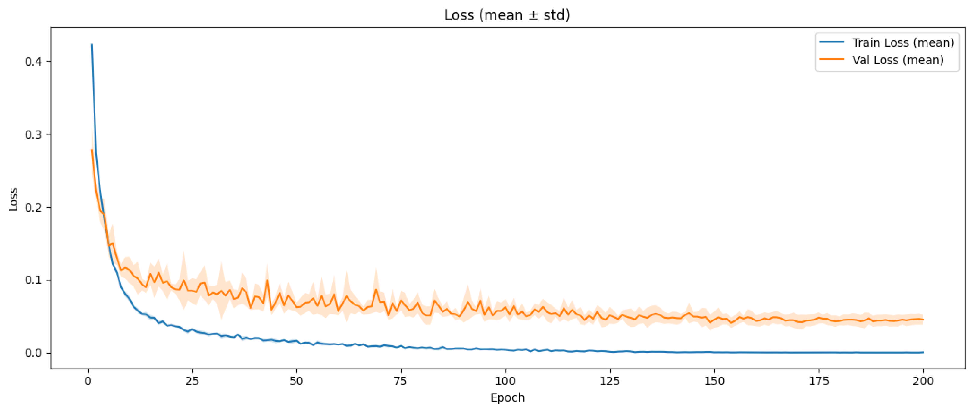
The accuracy curves in Figure 9 and Figure 10 indicate that training accuracy increased rapidly during the initial iterations and stabilized above 99%, while validation accuracy converged to 99.83% for Dataset I and 99.37% for Dataset II. Furthermore, as shown in Figure 11, the five-fold average results on Dataset III indicate that the model exhibits high stability during both training and validation phases. The training accuracy becomes stable after approximately 100 epochs, while the validation accuracy continues to improve and remains around 99.26% ± 0.16. For all three datasets, both training and validation losses show a sharp decline in the early stages and minimal fluctuations later, suggesting good convergence and no evident overfitting. Overall, these results demonstrate that the proposed model achieves stable learning behavior and excellent generalization performance across different data partitions.

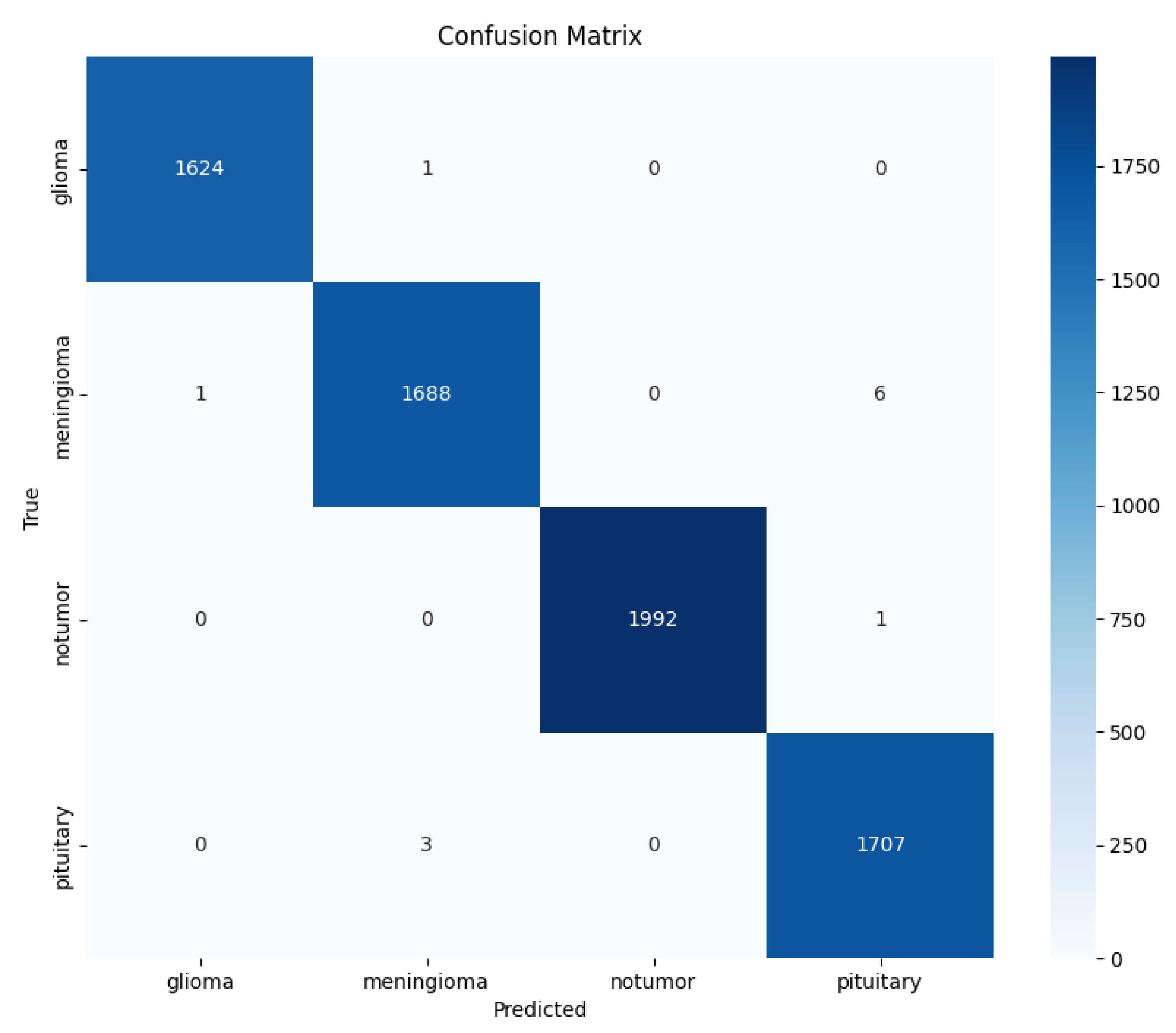
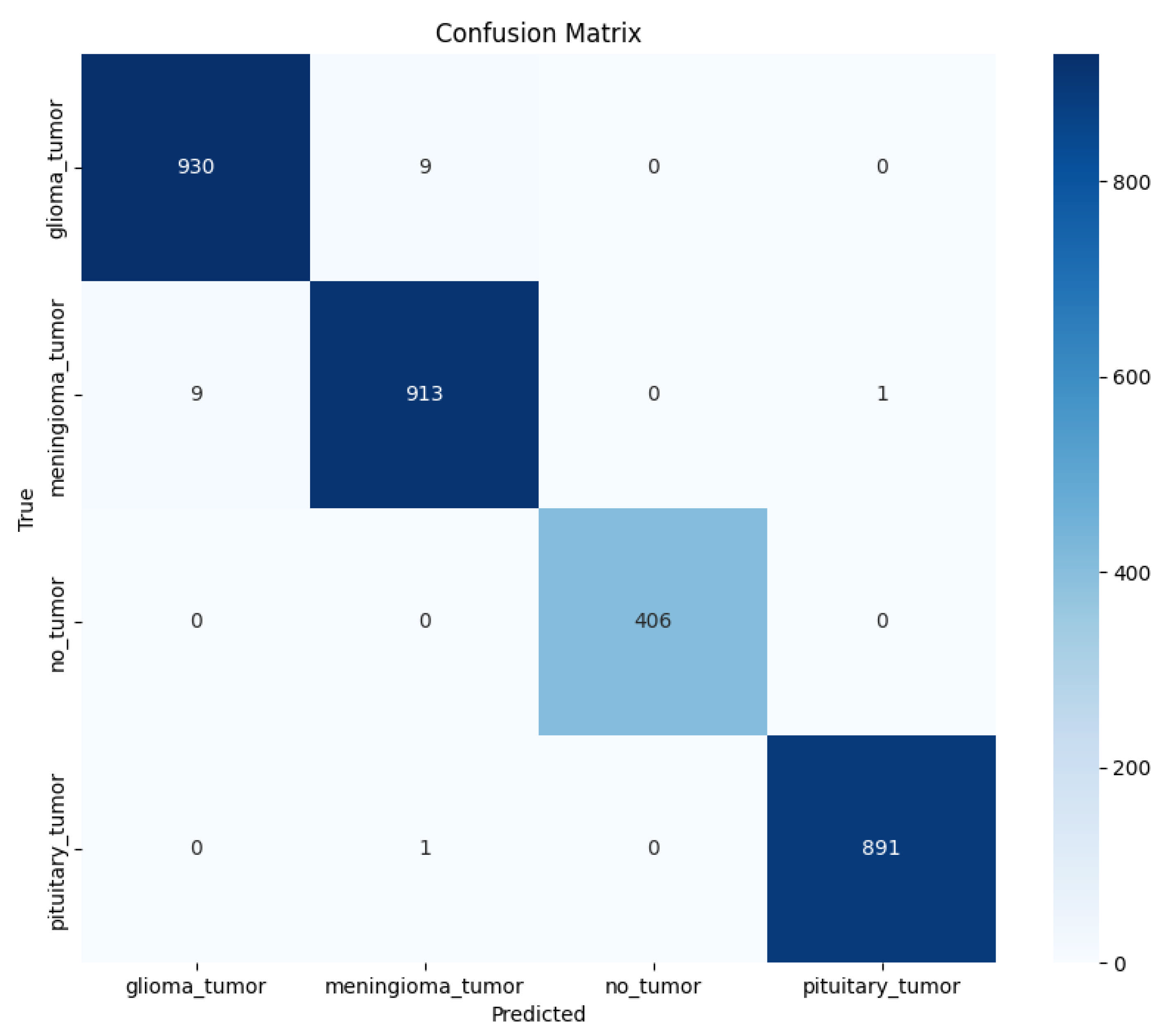
As illustrated in Figure 12 and Figure 13, the proposed model demonstrates stable and superior classification performance across the four brain tumor categories: glioma, men-ingioma, pituitary tumor, and no tumor. On Dataset I, the model correctly classifies 1624 glioma, 1688 meningioma, 1992 no-tumor, and 1707 pituitary images, with only a few misclassifications mainly occurring between meningioma and pituitary. Similarly, on Dataset II, the model achieves comparable results, correctly identifying 930 glioma, 913 meningioma, 406 no-tumor, and 891 pituitary images, with minimal confusion observed between glioma and meningioma. The strong diagonal dominance observed in both con-fusion matrices highlights the model’s excellent discriminative capability, high sensitivity, and robust generalization across different datasets.

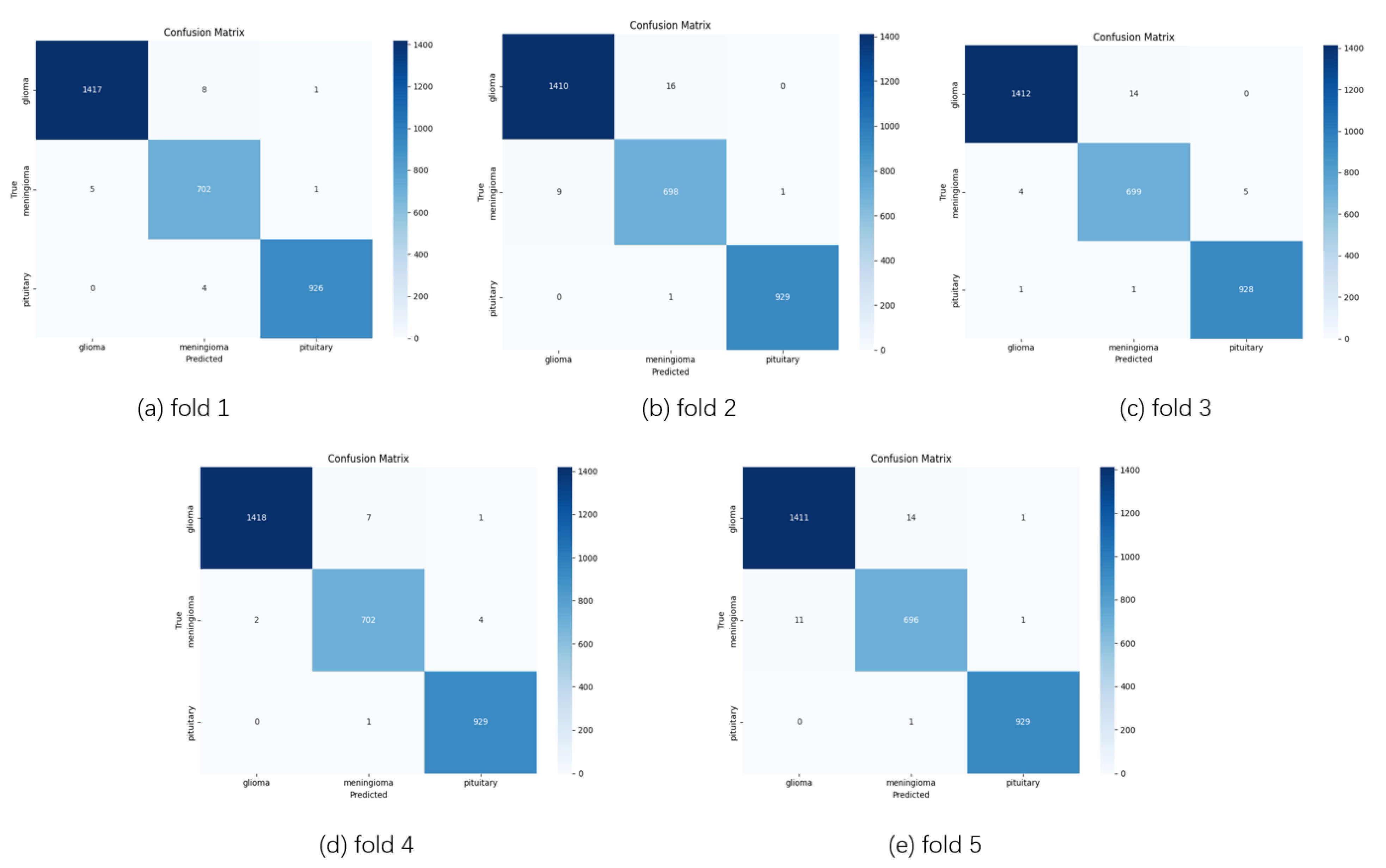
Figure 14 illustrates the predictive performance of the model on the brain tumor classification task using Dataset III under five-fold cross-validation. The confusion matrix for each fold evaluates the three tumor classes: glioma, meningioma, and pituitary. Overall, the model achieves high classification accuracy across most folds, with particularly stable performance in distinguishing pituitary tumors. Some degree of confusion between glioma and meningioma is observed, especially in folds 4 and 5, where a portion of glioma samples were misclassified as meningioma. This suggests that these two tumor types may share highly similar imaging features, making boundary cases more challenging for the model. Nevertheless, the overall misclassification rate remains low, indicating that the model possesses strong capability and robustness in feature extraction and class discrimination.

Collectively, these results confirm that the S-ResGCN model not only achieves high classification accuracy but also maintains robust stability and generalization, effectively handling MRI images with diverse tumor types and varying levels of complexity.

3.2. Comparison with Baseline Methods

The proposed S-ResGCN was evaluated on Brain Tumor MRI Dataset I, with its performance summarized in

Table 2. Experimental Results for Brain Tumor MRI Dataset I.

Methods	Accuracy	Precision	Recall	F1-Score
MobileNetV2 [27]	0.8445	0.8498	0.8445	0.8431
ResNet-18 [27]	0.8659	0.8658	0.8659	0.8635
VGG16 [27]	0.9497	0.9495	0.9497	0.9494
CBAM-CNN [28]	0.9670	0.9675	0.9650	0.9675
Inception V3 [29]	0.9712	0.9797	–	–
Pat-GridMask [30]	0.9774	–	–	0.9775
Custom CNN [31]	0.9809	0.9820	0.9810	0.9815
FTVT-132 [32]	0.9870	0.9870	0.9870	0.9870
S-ResGCN	0.9983	0.9982	0.9982	0.9982

, and compared against a range of representative models, including lightweight networks, classic CNNs, attention-enhanced architectures, multi-scale networks, and Transformer-based approaches. MobileNetV2 and ResNet-18 achieved moderate accuracies of 84.45% and 86.59%, respectively, while VGG16 improved to 94.97%. The incorporation of attention mechanisms further enhanced performance, as demonstrated by CBAM-CNN with an accuracy of 96.70%. Deeper or multi-scale architectures, such as Inception V3, Pat-GridMask, and Custom CNN, achieved 97–98% accuracy, whereas the Transformer-based FTVT-132 reached 98.70%.

In contrast, S-ResGCN attained 99.83% across all evaluation metrics, including accuracy, precision, recall, and F1-score, outperforming all baseline methods. This result highlights the effectiveness of hierarchical feature extraction, self-paired regularization, and graph convolutional modeling in capturing fine-grained and symmetric tumor characteristics, which are often overlooked by conventional models.

Table 3. Experimental Results on Brain Tumor MRI Dataset II.

Methods	Accuracy	Precision	Recall	F1-Score
Swin Transformer [33]	0.8888	0.8600	0.7500	0.8700
MSCNN [34]	0.9120	0.9200	0.9070	0.9100
HDL2BT [35]	0.9213	0.9213	–	–
CNN [36]	0.9330	–	0.9113	–
EfficientNet B7 [37]	0.9500	0.9300	0.9200	0.9300
CustomEfficientNet [38]	0.9700	0.9600	0.9600	0.9600
TLAEN [39]	0.9700	0.9700	0.9700	0.9700
Innovation CNN [40]	0.9820	–	–	–
S-ResGCN	0.9937	0.9946	0.9946	0.9946

presents the classification results on Brain Tumor MRI Dataset II. The proposed S-ResGCN achieved an accuracy of 99.37%, with mean precision, recall, and F1-score all reaching 99.46%, substantially outperforming baseline methods such as Swin Transformer (88.88%), MSCNN (91.20%), HDL2BT (92.13%), and a conventional CNN (93.30%). It also surpassed advanced architectures including EfficientNet-B7 (95.00%), CustomEfficientNet (97.00%), and TLAEN (97.00%), as well as the previously best-performing Innovation CNN (98.20%), achieving nearly 1% higher accuracy while maintaining superior robustness across all metrics. These results indicate that S-ResGCN exhibits remarkable capability in capturing fine-grained features, precise boundary delineation, and minority-class recognition.

The superior performance of S-ResGCN arises from its combination of hierarchical feature extraction, attention-enhanced symmetric feature learning via CBAM, self-paired regularization to enforce symmetry consistency, and a GCN-based head that captures inter-node relationships, collectively enabling more robust and fine-grained brain tumor classification than baseline models.

As shown in

Table 4. Experimental Results on Brain Tumor MRI Dataset III.

Methods	Accuracy	Precision	Recall	F1-Score
InceptionV3 [41]	0.9286	0.9270	0.9170	0.9200
DenseNet201 [41]	0.9481	0.9400	0.9400	0.9360
VGG16-NADE [42]	0.9601	0.9572	0.9564	0.9568
CNN [43]	0.9727	–	0.9113	–
MobDenseNet [44]	0.9840	0.9860	0.9840	0.9850
Innovation CNN [41]	0.9870	0.9830	0.9860	0.9860
S-ResGCN	0.9926 ± 0.16	0.9912	0.9924	0.9918

, compared with traditional convolutional neural networks such as InceptionV3 and DenseNet201, S-ResGCN exhibits a significant improvement in both classification accuracy and result stability. This advantage mainly stems from the Symmetry-aware Residual Graph Convolution, which jointly captures local spatial details and inter-hemispheric structural relationships, enhancing the model’s ability to discriminate lesions with blurred boundaries or similar morphology. In addition, the Attention-guided Feature Refinement module adaptively emphasizes tumor-relevant channels and suppresses redundant information, leading to more discriminative and robust feature representations that conventional CNNs often fail to achieve.

Furthermore, compared with the densely connected VGG16-NADE and the lightweight fusion-based MobDenseNet, S-ResGCN incorporates a Self-Paired Regularization (SPR) strategy that constrains bilateral brain feature consistency at the representation level, effectively reducing overfitting to asymmetric lesions during training. By enforcing structural symmetry consistency in the latent space, SPR further enhances the model’s generalization and stability across different subjects and scanning conditions.

3.3. Ablation Studies

An ablation study on Brain Tumor MRI Dataset II (

Table 5. Impacts of CBAM, SPR and GCN on Classification Accuracy.

Exp	CBAM	SPR	GCN	Accuracy	Precision	Recall	F1-Score
1				0.9573	0.9504	0.9642	0.9565
2			✓	0.9699	0.9695	0.9729	0.9710
3	✓			0.9747	0.9763	0.9785	0.9772
4		✓		0.9684	0.9635	0.9699	0.9665
5	✓		✓	0.9810	0.9827	0.9828	0.9827
6		✓	✓	0.9794	0.9683	0.9805	0.9740
7	✓	✓		0.9842	0.9847	0.9836	0.9841
8	✓	✓	✓	0.9937	0.9946	0.9946	0.9946

) was conducted to evaluate the individual and combined contributions of S-ResGCN’s core components. The baseline ResNet50 backbone achieved an accuracy of 95.73%, indicating limited capability in detecting small or poorly defined lesions. Incorporating the GCN head increased accuracy to 96.99%, demonstrating that graph-based relational modeling effectively strengthens spatial reasoning by aggregating features from both the original and horizontally flipped images. Adding CBAM further improved accuracy to 97.47%, highlighting its capacity to adaptively emphasize informative channels and spatial regions critical for tumor localization. Employing SPR loss alone yielded 96.84% accuracy, confirming that enforcing symmetry consistency enhances robustness to subtle and symmetric tumor structures.

Combining two components resulted in additional performance gains. The combination of the CBAM and GCN achieved 98.10% accuracy by effectively integrating attention-guided feature selection with graph-based relational modeling. CBAM combined with SPR reached 97.94% accuracy, leveraging the synergy between attention mechanisms and symmetry-aware regularization to improve lesion detection. The combination of GCN and SPR achieved 98.42% accuracy, reinforcing both spatial reasoning and symmetry consistency to better discriminate small lesions. The full integration of CBAM, GCN, and SPR achieved the highest accuracy of 99.37%, demonstrating that attention mechanisms, graph-based modeling, and symmetry regularization are complementary, jointly delivering substantial improvements in classification accuracy and the recognition of fine-grained tumor structures.

4. Conclusions

In this study, we proposed S-ResGCN, a symmetry-aware framework for brain tumor MRI classification that integrates hierarchical feature extraction, self-paired regularization, and a graph convolutional head. By jointly leveraging original and horizontally flipped images, the model enhances sensitivity to symmetric and discriminative tumor structures, while Convolutional Block Attention Module (CBAM) modules effectively emphasize critical lesion regions. Experiments on two public MRI datasets demonstrated consistently high accuracy, precision, recall, and F1-scores, particularly for complex and symmetric lesions. These findings highlight S-ResGCN’s robustness and its potential as a foundation for automated, symmetry-sensitive diagnostic systems.

However, the network design of S-ResGCN has certain limitations. First, the model relies on 2D MRI slices during training and evaluation, which may limit its ability to capture complex 3D tumor morphology. Second, the benefits of SPR are more pronounced for tumors with strong symmetry, while irregularly shaped tumors see comparatively less improvement. Moreover, the multi-branch structure and GCN head increase computational complexity, posing challenges for real-time processing on large-scale clinical datasets. Clearly stating these limitations helps readers better understand the framework’s applicability and potential areas for improvement.In the future, we plan to extend S-ResGCN to multi-modal MRI data and cross-center datasets to improve generalization under diverse imaging conditions. Further exploration of semi-supervised learning may reduce dependence on labeled data, while optimizing computational efficiency could enable real-time clinical deployment. Additionally, incorporating 3D volumetric inputs may enhance its effectiveness for tumor monitoring and treatment planning.

References

1. Katti, G.; Ara, S.A.; Shireen, A. Magnetic resonance imaging (MRI)—A review. Int. J. Dent. Clin. 2011, 3, 65–70. [Google Scholar]
2. Doi, K. Computer-aided diagnosis in medical imaging: Historical review, current status and future potential. Comput. Med. Imaging Graph. 2007, 31, 198–211. [Google Scholar] [CrossRef]
3. Jakkula, V. Tutorial on Support Vector Machine (Svm); School of EECS, Washington State University: Pullman, WA, USA, 2006; Volume 37, p. 3. [Google Scholar]
4. Fang, K.; Wu, J.; Zhu, J.; Xie, B. Review of random forest methods. Stat. Inf. BBS 2011, 26, 32–38. [Google Scholar]
5. Guo, G.; Wang, H.; Bell, D.; Bi, Y.; Greer, K. KNN model-based approach in classification. In OTM Confederated International Conferences “On the Move to Meaningful Internet Systems”; Springer: Berlin/Heidelberg, Germany, 2003; pp. 986–996. [Google Scholar]
6. O’shea, K.; Nash, R. An introduction to convolutional neural networks. arXiv 2015, arXiv:1511.08458. [Google Scholar] [CrossRef]
7. Musa, M.N. MRI-based brain tumor classification using resnet-50 and optimized softmax regression. J. Infotel 2024, 16, 598–614. [Google Scholar] [CrossRef]
8. Ahmed, G.; Er, M.J.; Fareed, M.M.S.; Zikria, S.; Mahmood, S.; He, J.; Asad, M.; Jilani, S.F.; Aslam, M. Dad-net: Classification of alzheimer’s disease using adasyn oversampling technique and optimized neural network. Molecules 2022, 27, 7085. [Google Scholar] [CrossRef]
9. Nizamli, Y.A.; Filatov, A.Y. Improving transfer learning performance for abnormality detection in brain MRI images using feature optimization techniques. In Proceedings of the 2024 XXVII International Conference on Soft Computing and Measurements (SCM), St. Petersburg, Russia, 22–24 May 2024; pp. 432–435. [Google Scholar]
10. Haq, A.U.; Li, J.P.; Agbley, B.L.Y.; Khan, A.; Khan, I.; Uddin, M.I.; Khan, S. IIMFCBM: Intelligent integrated model for feature extraction and classification of brain tumors using MRI clinical imaging data in IoT-healthcare. IEEE J. Biomed. Health Inform. 2022, 26, 5004–5012. [Google Scholar] [CrossRef]
11. Wang, M.; Ren, Y.; Lin, Y.; Wang, S. The tightly super 3-extra connectivity and diagnosability of locally twisted cubes. Am. J. Comput. Math. 2017, 7, 127–144. [Google Scholar] [CrossRef]
12. Wang, S.; Wang, Y.; Wang, M. Connectivity and matching preclusion for leaf-sort graphs. J. Interconnect. Netw. 2019, 19, 1940007. [Google Scholar] [CrossRef]
13. Wang, M.; Xiang, D.; Qu, Y.; Li, G. The diagnosability of interconnection networks. Discret. Appl. Math. 2024, 357, 413–428. [Google Scholar] [CrossRef]
14. Jiang, J.; Wu, L.; Yu, J.; Wang, M.; Kong, H.; Zhang, Z.; Wang, J. Robustness of bilayer railway-aviation transportation network considering discrete cross-layer traffic flow assignment. Transp. Res. Part D Transp. Environ. 2024, 127, 104071. [Google Scholar] [CrossRef]
15. Wang, M.; Xiang, D.; Wang, S. Connectivity and diagnosability of leaf-sort graphs. Parallel Process. Lett. 2020, 30, 2040004. [Google Scholar] [CrossRef]
16. Xiang, D.; Hsieh, S.Y. G-good-neighbor diagnosability under the modified comparison model for multiprocessor systems. Theor. Comput. Sci. 2025, 1028, 115027. [Google Scholar]
17. Wang, M.; Lin, Y.; Wang, S. The connectivity and nature diagnosability of expanded k-ary n-cubes. RAIRO-Theor. Inform. Appl.-Inform. Théor. Appl. 2017, 51, 71–89. [Google Scholar] [CrossRef]
18. Wang, M.; Lin, Y.; Wang, S. The nature diagnosability of bubble-sort star graphs under the PMC model and MM* model. Int. J. Eng. Appl. Sci. 2017, 4, 55–56. [Google Scholar]
19. Wang, M.; Wang, S. Connectivity and diagnosability of center k-ary n-cubes. Discret. Appl. Math. 2021, 294, 98–107. [Google Scholar] [CrossRef]
20. Zarenia, E.; Akhlaghi Far, A.; Rezaee, K. Automated multi-class MRI brain tumor classification and segmentation using deformable attention and saliency mapping. Sci. Rep. 2025, 15, 8114. [Google Scholar] [CrossRef]
21. Woo, S.; Park, J.; Lee, J.Y.; Kweon, I.S. Cbam: Convolutional block attention module. In Proceedings of the European Conference on Computer Vision (ECCV), Munich, Germany, 8–14 September 2018; pp. 3–19. [Google Scholar]
22. Rahman, Z.; Zhang, R.; Bhutto, J.A. A symmetrical approach to brain tumor segmentation in MRI using deep learning and threefold attention mechanism. Symmetry 2023, 15, 1912. [Google Scholar] [CrossRef]
23. Zhang, S.; Tong, H.; Xu, J.; Maciejewski, R. Graph convolutional networks: A comprehensive review. Comput. Soc. Netw. 2019, 6, 11. [Google Scholar] [CrossRef]
24. Nickparvar, M. Brain Tumor MRI Dataset; Kaggle: San Francisco, CA, USA, 2021. [Google Scholar]
25. Sayedgomaa, S. Brain Tumor. Kaggle Notebook. 2022. Available online: https://www.kaggle.com/code/sayedgomaa/brain-tumor/notebook (accessed on 21 December 2022).
26. Cheng, J. Brain Tumor Dataset. 2017. Available online: https://figshare.com/articles/dataset/brain_tumor_dataset/1512427 (accessed on 20 October 2025).
27. Liu, X.; Wang, Z. Deep learning in medical image classification from mri-based brain tumor images. In Proceedings of the 2024 IEEE 6th International Conference on Power, Intelligent Computing and Systems (ICPICS), Shenyang, China, 26–28 July 2024; pp. 840–844. [Google Scholar]
28. Binish, M.; Raj, R.S.; Thomas, V. Brain tumor classification using multi-resolution averaged spatial attention features with CBAM and convolutional neural networks. In Proceedings of the 2024 1st International Conference on Trends in Engineering Systems and Technologies (ICTEST), Kochi, India, 11–13 April 2024; pp. 1–7. [Google Scholar]
29. Gómez-Guzmán, M.A.; Jiménez-Beristaín, L.; García-Guerrero, E.E.; López-Bonilla, O.R.; Tamayo-Perez, U.J.; Esqueda-Elizondo, J.J.; Palomino-Vizcaino, K.; Inzunza-González, E. Classifying brain tumors on magnetic resonance imaging by using convolutional neural networks. Electronics 2023, 12, 955. [Google Scholar] [CrossRef]
30. Lee, J.H.; Chae, J.W.; Cho, H.C. Improved classification of different brain tumors in mri scans using patterned-gridmask. IEEE Access 2024, 12, 40204–40212. [Google Scholar] [CrossRef]
31. Khan, M.A.; Auvee, R.B.Z. Comparative Analysis of Resource-Efficient CNN Architectures for Brain Tumor Classification. In Proceedings of the 2024 27th International Conference on Computer and Information Technology (ICCIT), Cox’s Bazar, Bangladesh, 20–22 December 2024; pp. 639–644. [Google Scholar]
32. Reddy, C.K.K.; Reddy, P.A.; Janapati, H.; Assiri, B.; Shuaib, M.; Alam, S.; Sheneamer, A. A fine-tuned vision transformer based enhanced multi-class brain tumor classification using MRI scan imagery. Front. Oncol. 2024, 14, 1400341. [Google Scholar] [CrossRef] [PubMed]
33. Zahoor, A.; Irfan, M.; Usman, M.; Haider, W. Brain tumor detection in magnetic resonance images using swin transformer. Conclus. Med. 2025, 1, 1–5. [Google Scholar] [CrossRef]
34. Yazdan, S.A.; Ahmad, R.; Iqbal, N.; Rizwan, A.; Khan, A.N.; Kim, D.H. An efficient multi-scale convolutional neural network based multi-class brain MRI classification for SaMD. Tomography 2022, 8, 1905–1927. [Google Scholar] [CrossRef]
35. Khan, A.H.; Abbas, S.; Khan, M.A.; Farooq, U.; Khan, W.A.; Siddiqui, S.Y.; Ahmad, A. Intelligent model for brain tumor identification using deep learning. Appl. Comput. Intell. Soft Comput. 2022, 2022, 8104054. [Google Scholar] [CrossRef]
36. Mahmud, M.I.; Mamun, M.; Abdelgawad, A. A deep analysis of brain tumor detection from mr images using deep learning networks. Algorithms 2023, 16, 176. [Google Scholar] [CrossRef]
37. Wibowo, M.P.; Al Fayyadl, M.B.; Azhar, Y.; Sari, Z. Classification of brain tumors on mri images using convolutional neural network model efficientnet. J. RESTI (Rekayasa Sist. Teknol. Informasi) 2022, 6, 538–547. [Google Scholar] [CrossRef]
38. Ishaq, A.; Ullah, F.U.M.; Hamandawana, P.; Cho, D.J.; Chung, T.S. Improved EfficientNet architecture for multi-grade brain tumor detection. Electronics 2025, 14, 710. [Google Scholar] [CrossRef]
39. SHARMA, P.; SHUKLA, A.P. Transfer learning approach using efficientnet architecture for brain tumor classification in Mri images. Adv. Appl. Math. Sci. 2022, 21, 7091–7106. [Google Scholar]
40. Ramadhani, M.R.; Soesanti, I.; Hidayah, I. Brain Tumor Classification Based on Deep Learning Algorithms. In Proceedings of the 2024 4th International Conference on Electronic and Electrical Engineering and Intelligent System (ICE3IS), Yogyakarta, Indonesia, 7–8 August 2024; pp. 81–86. [Google Scholar]
41. Ait Amou, M.; Xia, K.; Kamhi, S.; Mouhafid, M. A novel MRI diagnosis method for brain tumor classification based on CNN and Bayesian Optimization. Healthcare 2022, 10, 494. [Google Scholar] [CrossRef]
42. Sowrirajan, S.R.; Balasubramanian, S.; Raj, R.S.P. MRI brain tumor classification using a hybrid VGG16-NADE model. Braz. Arch. Biol. Technol. 2022, 66, e23220071. [Google Scholar] [CrossRef]
43. Sadr, H.; Nazari, M.; Yousefzade-Chabok, S.; Emami, H.; Rabiei, R.; Ashraf, A. Enhancing brain tumor classification in MRI images: A deep learning-based approach for accurate classification and diagnosis. Image Vis. Comput. 2025, 159, 105555. [Google Scholar] [CrossRef]
44. Afroj, M.; Mondal, M.R.H.; Hassan, M.R.; Akter, S. MobDenseNet: A Hybrid Deep Learning Model for Brain Tumor Classification Using MRI. Array 2025, 26, 100413. [Google Scholar] [CrossRef]
Figure 1. Brain tumor types: glioma, meningioma, no tumor, and pituitary.
Symmetry 17 01946 g001
Figure 2. S-ResGCN Model Architecture.
Symmetry 17 01946 g002
Figure 3. Convolutional Block Attention Module Heatmap.
Symmetry 17 01946 g003
Figure 4. (a) Channel Attention Module, which uses an MLP to highlight important feature channels. (b) Spatial Attention Module, which focuses on key regions in the feature map using a convolutional layer. (c) Convolutional Block Attention Module (CBAM), which sequentially applies the channel and spatial attention mechanisms from (a,b) to refine the input features, combining both for enhanced feature representation.
Symmetry 17 01946 g004
Figure 5. Visualization of the Self-Paired Regularization (SPR) loss. The figure illustrates how SPR enhances symmetry-aware feature learning in brain MRI. The first panel presents the original MRI image, while the second and third panels show the feature maps extracted by the backbone network from the original and horizontally flipped images, respectively. The fourth panel visualizes the absolute difference | x flip ( x ) | between the two feature maps, highlighting regions where symmetry is not fully preserved.
Symmetry 17 01946 g005
Figure 6. Classification report on dataset I.
Symmetry 17 01946 g006
Figure 7. Classification report on dataset II.
Symmetry 17 01946 g007
Figure 8. Classification report on dataset III.
Symmetry 17 01946 g008
Figure 9. Loss and accuracy curves on dataset I.
Symmetry 17 01946 g009
Figure 10. Loss and accuracy curves on dataset II.
Symmetry 17 01946 g010
Figure 11. Mean Loss and accuracy curves on dataset III.
Symmetry 17 01946 g011aSymmetry 17 01946 g011b
Figure 12. The results of the confusion matrix model on dataset I.
Symmetry 17 01946 g012
Figure 13. The results of the confusion matrix model dataset II.
Symmetry 17 01946 g013
Figure 14. The results of the confusion matrix model dataset III.
Symmetry 17 01946 g014