Estimating Unknown Parameters and Disturbance Term in Uncertain Regression Models by the Principle of Least Squares

Abstract

In the field of statistics, uncertain regression analysis occupies an important position. It can thoroughly analyze data sets contained in complex uncertainties, aiming to quantify and reveal the intricate relationships between variables. It is worth noting that the traditional least squares method only takes into account the reduction in the deviations between predictions and observations, and fails to fully consider the inherent characteristics of the correlation uncertainty distributions under the uncertain regression framework. In light of this, this paper constructs a statistical invariant with symmetric uncertainty distribution based on the observations and the disturbance term. It also proposes the least squares estimation of unknown parameters and disturbance term in the uncertain regression model based on the least squares principle and, combined with the mathematical properties of the normal uncertainty distribution, gives a numerical algorithm for solving specific estimates. Finally, in order to verify the effectiveness of the least squares estimation method proposed in this paper, we also design two numerical examples and an empirical study of forecasting of electrical power output.

1. Introduction

Regression analysis, as a core analysis tool in statistics, plays an important role in the field of statistics. Its core lies in exploring the intrinsic relationship between one or more independent variables (i.e., explanatory variables) and dependent variables (i.e., response variable). Tracing back to its historical origins, the budding of regression analysis can be attributed to the pioneering work of Francis Galton, an outstanding British statistician in the 19th century. Through the research on family height inheritance, Galton [1] revealed that although parents’ height has a significant impact on their children, their children’s heights tend to “regress” to the average height of the population. This discovery laid the initial foundation for regression analysis. Over time, regression analysis has flourished under the unremitting efforts of many statisticians, and a series of important model variants have emerged, including but not limited to logistic regression (theoretical foundation laid by Berkson [2]), ridge regression (the outstanding contribution of Hoerl and Kennard [3]), lasso regression (the innovative work of Tibshirani [4]), and elastic net regression (joint research of Zou and Hastie [5]). These models have greatly enriched the theoretical system of regression analysis and made it occupy an indispensable position in modern statistics. For readers who want to gain a deeper understanding of regression analysis and its latest developments, the works by Freund et al. [6], Sen and Srivastava [7], and Chatterjee and Simonoff [8] are undoubtedly valuable resources. They not only elaborate on the basic principles and applications of regression analysis, but also explore the latest research results and development trends in this field.

The traditional regression model is based on the assumption that the frequency of observed data is stable. It aims to analyze the intrinsic relationship between the explanatory variables and the response variable, and to characterize environmental uncertainty by abstracting it as random variables. However, the real world is complex and dynamic, and is frequently hit by unpredictable events such as natural disasters, political changes, and economic fluctuations, which often lead to abnormal fluctuations and frequency non-stationary phenomena in data records, setting up many obstacles for data analysis and future predictions. In view of this, deep insight into and acceptance of data instability is a necessary prerequisite for regression analysis and modeling, and targeted strategies are needed to address and explain these complex properties. In this context, redefining environmental uncertainty as uncertain variables not only suits the reality, but also provides a theoretical basis and practical opportunities for the emerging method of uncertain regression analysis, showing a broad prospect as a powerful supplement to traditional methods. In the framework of uncertain regression analysis, uncertain phenomena in practice are characterized as specific uncertain variables. As a statistical methodology, this analysis system abandons the foundation of traditional probability theory and is rooted in uncertainty theory (see the research of Liu [9] and Liu [10]). Over the years, the academic community has actively explored the integration of statistical regression methods with uncertainty theory, which has spawned a variety of uncertain regression models and research methods, and these results have shown their practical application values in many disciplines.

As a tool, uncertain regression analysis can deeply analyze the relationship between variables. Its theoretical basis can be traced back to the pioneering work of Yao and Liu [11]. They innovatively regarded the disturbance term as an uncertain variable rather than a random variable, which pointed out the direction for subsequent related research. Since then, uncertain regression models have continued to develop and enrich. For example, Ye and Liu [12] designed a multivariate uncertain regression model for the complex situation of multivariate response variables, realizing the simultaneous analysis of the relationship between multiple variables. In the face of unknown information that may be hidden in the error term, Chen [13] and Chen [14] introduced uncertain regression models with autoregressive time series errors and moving average time series errors, respectively, aiming to more accurately mine error information and improve prediction accuracy. For panel data containing temporal and spatial characteristics, Jiang and Ye [15] innovatively constructed an uncertain panel regression model, which spans the two dimensions of time and space and thoroughly reveals the complex interactive relationships hidden in panel data. In addition, Ding and Zhang [16] focused on the uncertain nonparametric regression model, which showed excellent adaptability and analytical efficiency in the case of unclear parameter forms. This series of studies not only expanded the theoretical boundaries of uncertain regression analysis, but also provided a wider and more flexible choice for its application in practical problems. Beyond that, the statistical inference of an uncertain regression model is another core issue in its research, and its key tasks mainly focus on two aspects: one is to accurately solve the unknown parameters in the model, and the other is to effectively estimate the uncertain disturbance term of the model. Regarding the determination of unknown parameters, Yao and Liu [11] first introduced the least squares estimation method, whose essence is to minimize the sum of squares of the differences between the predicted and observed values, but this method is susceptible to abnormal data. Subsequently, Liu and Yang [17] turned to the least absolute deviations estimation to cope with the challenge of outliers. Lio and Liu [18] took a different approach, incorporating the concept of the likelihood function and proposed uncertain maximum likelihood estimation. Chen [19] explored the Tukey’s biweight estimation and used the biweight loss function to optimize parameter estimation. Liu [20] derived the moment estimation by constructing statistical invariants, while Xie et al. [21] developed the Huber estimation based on the Huber loss function. For the estimation of the uncertain disturbance term, Lio and Liu [22] initially tried the moment estimation method. Subsequently, Lio and Liu [18] further introduced the uncertain maximum likelihood estimation. In the face of outlier problems in the data, Liu and Liu [23] adjusted this method to improve its robustness. At the same time, Liu and Liu [24] also proposed the least squares estimation method based on minimizing the sum of squared deviations between the empirical distribution of the observations and the population distribution for the estimation of the disturbance term. The applications of uncertain regression analysis have widely covered multiple fields, including but not limited to infectious disease analysis (Liu [25], Yang [26], Ding and Ye [27]), agricultural production (Li et al. [28]), population dynamics (Liu [29], Gao et al. [30]), carbon emission research (Chen and Yang [31]), and economic and financial modeling (Ye and Liu [32], Jia and Tang [33]), demonstrating its strong practical value and theoretical depth.

Although some scholars have studied the least squares estimation of unknown parameters and the least squares estimation of the disturbance term in uncertain regression models, they have not considered the estimations of unknown parameters and disturbance term at the same time, nor have they fully considered the correlation between observation data and the disturbance term. In view of this, this paper constructs a statistical invariant with symmetric uncertainty distribution based on the observation data and disturbance term, and proposes the least squares estimations of unknown parameters and disturbance term in uncertain regression models using the least squares principle. Specifically, the main contributions of this paper are as follows:

• This paper constructed a statistical invariant with symmetric uncertainty distribution based on the observation data and disturbance term, and applied the least squares principle to estimate unknown parameters and the uncertain disturbance term in the uncertain regression model.
• A numerical algorithm was designed to solve the specific estimator.
• Two numerical examples and an empirical case study of forecasting of electrical power output were provided to illustrate the method proposed in this paper.

2. Estimating Unknown Parameters and Disturbance Term in Uncertain Regression Model

In this section, we will study the parameter estimation problem in uncertain regression analysis based on the principle of least squares, including determining the unknown parameters and disturbance term of the uncertain regression models.

2.1. Least Squares Estimator

Assume that we have a series of observations $x_1,x_2,\cdots ,x_n$ derived from a population whose uncertainty distribution is ${\mathsf{\Phi }}_{\theta }$, where $\theta$ is a vector containing unknown parameters. In order to estimate the population distribution ${\mathsf{\Phi }}_{\theta }$ based on the observations $x_1,x_2,\cdots ,x_n$ such that the estimated population distribution fits the observations well, Liu and Liu [24] studied the least squares estimation of $\theta$ by means of minimizing the sum of squares of the deviation between the empirical distribution of observations and the population distribution. That is, the least squares estimation of $\theta$ solves the following optimization problem:

$$\underset{\theta }{min}\sum _{i=1}^n{\left({\mathsf{\Phi }}_{\theta }\left(x_i\right)-F\left(x_i\right)\right)}^2,$$

(1)

where

$$F\left(x\right)={\displaystyle \frac{1}{n}}\sum _{i=1}^n\mathbb{I}(x_i\le x)$$

is the empirical distribution of observations $x_1,x_2,\cdots ,x_n$, where $\mathbb{I}$ represents the indicator function, i.e.,

$$\mathbb{I}(x_i\le x)=\left\{\begin{array}{cc}{\displaystyle 1}\hfill & \mathrm{if}{x}_i\le x\hfill \\ {\displaystyle 0}\hfill & \mathrm{otherwise}.\hfill \end{array}\right.$$

Meanwhile, if the population distribution ${\mathsf{\Phi }}_{\theta }$ is a normal uncertainty distribution $\mathcal{N}(e,\sigma )$ with e and $\sigma >0$, Liu and Liu [24] also declared that the least squares estimation of $(e,\sigma )$ solves the minimization problem below:

$$\underset{e,\sigma >0}{min}\sum _{i=1}^n{\left({\left(1+exp\left({\displaystyle \frac{\pi (e-x_i)}{\sqrt{3}\sigma }}\right)\right)}^{-1}-{\displaystyle \frac{1}{n}}\sum _{j=1}^n\mathbb{I}(x_j\le x_i)\right)}^2.$$

(2)

2.2. Least Squares Estimation of Uncertain Regression Model

In the framework of regression analysis, it is usually assumed that the explanatory variables are in the form of $(x_1,x_2,\cdots ,x_p)$, and the response variable is denoted by y. In order to deeply analyze how these explanatory variables work together on the response variable under uncertain environments, Yao and Liu [11] constructed an uncertain regression model

$$y=f(x_1,x_2,\cdots ,x_p|\beta )+\epsilon$$

(3)

by depicting the uncertain factors affecting the relationship between variables as uncertain variables. Here, f is a real function representing the relationship between variables, while $\beta$ is an unknown parameter vector, and $\epsilon$ is assumed as an uncertain disturbance term whose expected value is 0 and standard deviation is $\sigma$, denoted as $\mathcal{N}(0,\sigma )$.

Assume that we have a series of observations:

$$(x_{i1},x_{i2},\cdots ,x_{ip},y_i),i=1,2,\cdots ,n$$

about the explanatory variables $(x_1,x_2,\cdots ,x_p)$ and response variable y. If the unknown parameter vector $\beta$ and the standard deviation $\sigma$ of the uncertain disturbance term can both take the corresponding true values, then according to uncertain regression model (3), we can obtain

$$y-f(x_1,x_2,\cdots ,x_p|\beta )\sim \mathcal{N}(0,\sigma ),$$

which can be rearranged as

$${\displaystyle \frac{y-f(x_1,x_2,\cdots ,x_p|\beta )}{\sigma }}\sim \mathcal{N}(0,1).$$

By substituting the above observations into the above equation and writing

$$h_i(\beta ,\sigma )={\displaystyle \frac{y_i-f(x_{i1},x_{i2},\cdots ,x_{ip}|\beta )}{\sigma }}$$

for $i=1,2,\cdots ,n$, we can obtain n real functions of the unknown parameter vector $\beta$ and $\sigma$ as

$$h_1(\beta ,\sigma ),h_2(\beta ,\sigma ),\cdots ,h_n(\beta ,\sigma ),$$

which can be regarded as the samples of

$${\displaystyle \frac{y-f(x_1,x_2,\cdots ,x_p|\beta )}{\sigma }}.$$

That is, the above n real functions should be n samples of the uncertainty distribution $\mathcal{N}(0,1)$. In other words, we should have

$$h_1(\beta ,\sigma ),h_2(\beta ,\sigma ),\cdots ,h_n(\beta ,\sigma )\sim \mathcal{N}(0,1),$$

(4)

where the standard normal uncertainty distribution $\mathcal{N}(0,1)$ is the symmetric statistical invariant we construct.

Note that the empirical distribution of $h_1(\beta ,\sigma ),h_2(\beta ,\sigma ),\cdots ,h_n(\beta ,\sigma )$ is

$$F\left(x\right)={\displaystyle \frac{1}{n}}\sum _{i=1}^n\mathbb{I}(h_i(\beta ,\sigma )\le x),$$

and the uncertainty distribution of $\mathcal{N}(0,1)$ is

$$\mathsf{\Phi }\left(x\right)={\left(1+exp\left({\displaystyle \frac{-\pi x}{\sqrt{3}}}\right)\right)}^{-1}.$$

It follows from (1) that the least squares estimations of $\beta$ and $\sigma$ solve the following minimization problem:

$$\underset{\beta ,\sigma >0}{min}\sum _{i=1}^n{\left({\left(1+exp\left({\displaystyle \frac{-\pi h_i(\beta ,\sigma )}{\sqrt{3}}}\right)\right)}^{-1}-{\displaystyle \frac{1}{n}}\sum _{j=1}^n\mathbb{I}(h_j(\beta ,\sigma )\le h_i(\beta ,\sigma ))\right)}^2.$$

(5)

Because the core challenge of the optimization problem (5) lies in the nonlinear expression of decision variables in its objective function, it is often difficult to directly solve its optimal solution. To overcome this obstacle, we design and implement a specific algorithm that aims to effectively process and approximate the least squares solution to this optimization problem, which is Algorithm 1.

Algorithm 1: Numerical solutions of least squares estimators.

Step 0: Input observational data $$(x_{i1},x_{i2},\cdots ,x_{ip},y_i),i=1,2,\cdots ,n.$$ Step 1: Determine the feasible regions $\mathsf{\Theta }$ of unknown parameter vector $\beta$.

Step 2: For each $\beta \in \mathsf{\Theta }$ and $\sigma >0$, compute $h_1(\beta ,\sigma ),h_2(\beta ,\sigma ),\cdots ,h_n(\beta ,\sigma )$ by $$h_i(\beta ,\sigma )={\displaystyle \frac{y_i-f(x_{i1},x_{i2},\cdots ,x_{ip}|\beta )}{\sigma }},i=1,2,\cdots ,n.$$ Step 3: Set $i=1$ and $E\left(\beta ,\sigma \right)=0$.

Step 4: Set $$E\left(\beta ,\sigma \right)=E\left(\beta ,\sigma \right)+{\left({\left(1+exp\left({\displaystyle \frac{-\pi h_i(\beta ,\sigma )}{\sqrt{3}}}\right)\right)}^{-1}-{\displaystyle \frac{1}{n}}\sum _{j=1}^n\mathbb{I}(h_j(\beta ,\sigma )\le h_i(\beta ,\sigma ))\right)}^2,$$ and $i=i+1$.

Step 5: If $i\le n$, then go to Step 4.

Step 6: Find $\widehat{\beta }$ and $\widehat{\sigma }$ such that $E\left(\beta ,\sigma \right)$ reaches its minimum value.

Step 7: Output $\widehat{\beta }$ and $\widehat{\sigma }$.

3. Hypothesis Test and Forecast

Based on the estimated parameters and disturbance term, we can obtain an estimated uncertain regression model:

$$y=f(x_1,x_2,\cdots ,x_p|\widehat{\beta })+\mathcal{N}(0,\widehat{\sigma }).$$

(6)

Then the following core problems involve determining whether the estimated uncertain regression model (6) is reasonable and how to forecast the response variable based on the new explanatory variables.

3.1. Uncertain Hypothesis Test

First, we need to determine whether the estimated uncertain regression model (6) is reasonable. In other words, we should answer the question of whether the estimated uncertain regression model (6) fits the given observation data set well.

In order to evaluate the applicability of this estimated model, we can calculate the corresponding residual sequence according to

$${\epsilon }_i=y_i-f(x_{i1},x_{i2},\cdots ,x_{ip}|\widehat{\beta }),i=1,2,\cdots ,n.$$

For the n residual terms ${\epsilon }_1,{\epsilon }_2,\cdots ,{\epsilon }_n$, they reflect the differences between the forecast values based on the estimated model and the actual observations. Next, the key to verifying whether the estimated model can fit the given observation data set well is to test whether this set of residual sequence follows the normal uncertainty distribution $\mathcal{N}(0,\widehat{\sigma })$. This involves a hypothesis test on the standard deviation of the normal uncertainty distribution $\mathcal{N}(0,\widehat{\sigma })$, and the specific hypothesis is

$$H_0:\sigma =\widehat{\sigma } \mathrm{versus} H_1:\sigma \ne \widehat{\sigma }.$$

(7)

Setting a specific significance threshold $\alpha$, the work of Ye and Liu [34] recommended a test for the above hypothesis (7) as a strategy to verify whether the null hypothesis $H_0$ holds, which is

$$\begin{array}{cc}\hfill W=\left\{\right(z_1,z_2,\cdots ,z_n):& \mathrm{there} \mathrm{are} \mathrm{at} \mathrm{least} \lfloor n\times \alpha +1\rfloor \mathrm{of} \mathrm{indexes} i^{\prime }\mathrm{s} \mathrm{with} 1\le i\le n\hfill \\ \hfill & \mathrm{such} \mathrm{that} z_i<{\mathsf{\Phi }}^{-1}\left({\displaystyle \frac{\alpha }{2}}\right) \mathrm{or} z_i>{\mathsf{\Phi }}^{-1}\left({\displaystyle 1-\frac{\alpha }{2}}\right)\},\hfill \end{array}$$

(8)

where $\lfloor x\rfloor$ indicates the largest integer not greater than x, and

$${\mathsf{\Phi }}^{-1}\left(\alpha \right)={\displaystyle \frac{\sqrt{3}\widehat{\sigma }}{\pi }}ln{\displaystyle \frac{\alpha }{1-\alpha }}.$$

Through this test, we can evaluate whether the obtained residual sequence ${\epsilon }_1,{\epsilon }_2,\cdots ,{\epsilon }_n$ follows the normal uncertainty distribution $\mathcal{N}(0,\widehat{\sigma })$, so as to judge whether the estimated uncertain regression model (6) is a good fit to the observation data set. In detail, if the obtained residual sequence belongs to the test W, i.e.,

$$({\epsilon }_1,{\epsilon }_2,\cdots ,{\epsilon }_n)\in W,$$

then it is not enough to simply use a normal uncertainty distribution with a mean of 0 and a standard deviation of $\widehat{\sigma }$ to characterize this set of residuals. In this case, the estimated uncertain regression model (6) is difficult to directly achieve an ideal fit of the observation data set. On the contrary, if the above conditions are not satisfied, it can be reasonably inferred that the estimated uncertain regression model (6) can better adapt to and fit the observation data set.

3.2. Point Forecast and Interval Forecast

In this subsection, we will derive the point forecast and interval forecast for the response variable based on the estimated uncertain regression model (6) and given explanatory variables.

Assuming that the given explanatory variable is

$$({\widehat{x}}_1,{\widehat{x}}_2,\cdots ,{\widehat{x}}_p),$$

then according to the research results of Yao and Liu [11], the forecast uncertain variable of the response variable can be defined as

$$\widehat{y}=f({\widehat{x}}_1,{\widehat{x}}_2,\cdots ,{\widehat{x}}_p|\widehat{\beta })+\mathcal{N}(0,\widehat{\sigma })\sim \mathcal{N}(f({\widehat{x}}_1,{\widehat{x}}_2,\cdots ,{\widehat{x}}_p|\widehat{\beta }),\widehat{\sigma }),$$

whose uncertainty distribution is

$$\widehat{\mathsf{\Phi }}\left(x\right)={\displaystyle \frac{1}{1+exp\left({\displaystyle \frac{\pi (f({\widehat{x}}_1,{\widehat{x}}_2,\cdots ,{\widehat{x}}_p|\widehat{\beta })-x)}{\sqrt{3}\widehat{\sigma }}}\right)}}$$

and inverse uncertainty distribution is

$${\widehat{\mathsf{\Phi }}}^{-1}\left(\alpha \right)=f({\widehat{x}}_1,{\widehat{x}}_2,\cdots ,{\widehat{x}}_p|\widehat{\beta })+{\displaystyle \frac{\widehat{\sigma }\sqrt{3}}{\pi }}ln{\displaystyle \frac{\alpha }{1-\alpha }}.$$

In this case, we can take the expected value of the forecast uncertain variable $\widehat{y}$ as the point forecast value of the response variable, i.e.,

$$\widehat{\mu }={\int }_0^1{\widehat{\mathsf{\Phi }}}^{-1}\left(\alpha \right)\mathrm{d}\alpha =f({\widehat{x}}_1,{\widehat{x}}_2,\cdots ,{\widehat{x}}_p|\widehat{\beta }).$$

(9)

Further, assuming that $\alpha$ (e.g., 95%) is a given confidence level, then we can derive

$$\begin{array}{cc}\hfill & \mathrm{M}\left\{{\widehat{\mathsf{\Phi }}}^{-1}\left({\displaystyle \frac{1-\alpha }{2}}\right)\le \widehat{y}\le {\widehat{\mathsf{\Phi }}}^{-1}\left({\displaystyle \frac{1+\alpha }{2}}\right)\right\}\hfill \\ \hfill \ge & {\widehat{\mathsf{\Phi }}}^{-1}\left({\widehat{\mathsf{\Phi }}}^{-1}\left({\displaystyle \frac{1+\alpha }{2}}\right)\right)-{\widehat{\mathsf{\Phi }}}^{-1}\left({\widehat{\mathsf{\Phi }}}^{-1}\left({\displaystyle \frac{1-\alpha }{2}}\right)\right)\hfill \\ \hfill =& \alpha .\hfill \end{array}$$

The above formula means that

$$\left[{\widehat{\mathsf{\Phi }}}^{-1}\left({\displaystyle \frac{1-\alpha }{2}}\right),{\widehat{\mathsf{\Phi }}}^{-1}\left({\displaystyle \frac{1+\alpha }{2}}\right)\right]$$

is a reasonable fluctuation range of the value of the response variable at the $\alpha$ confidence level. Therefore, we can choose the above interval, i.e.,

$$\widehat{\mu }\pm {\displaystyle \frac{\widehat{\sigma }\sqrt{3}}{\pi }}ln{\displaystyle \frac{1+\alpha }{1-\alpha }},$$

(10)

as the forecast interval ($\alpha$ confidence interval) of the response variable.

4. Numerical Examples

In this section, we aim to illustrate the method using the least squares principle to estimate the unknown parameters and disturbance term in the uncertain regression model through two numerical examples.

Example 1.

When exploring growth patterns in complex environments, one approach is to capture the trend of growth from slow to sharp acceleration by constructing an exponential model, especially in uncertain scenarios such as asset trends in early markets or the spread of early cases of infectious diseases. The specific exponential growth model is as follows:

$$\begin{array}{c}\hfill y={\beta }_0+{\beta }_{1}exp\left({\beta }_{2}x\right)+\epsilon ,\end{array}$$

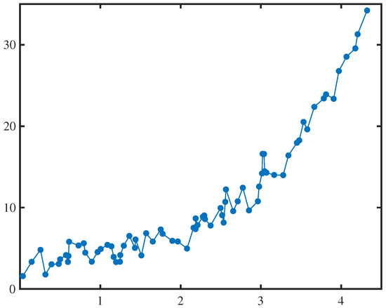
where ${\beta }_0$, ${\beta }_1$, and ${\beta }_2$ are the parameters to be estimated, and ε is an uncertain disturbance term, which is assumed to follow a normal uncertainty distribution with a mean of 0 and a standard deviation of σ. In addition, for the empirical analysis, we assume that there is a data set containing 76 sets of observations, which are related to the explanatory variables and the response variable, and are presented in the form of Table 1 and Figure 1.

Table 1. Observational data of Example 1.

x	y	x	y	x	y	x	y
0.0350	1.5892	1.1663	3.9409	2.1875	8.6692	3.0388	16.5826
0.1450	3.3379	1.1963	3.3124	2.2113	7.8528	3.0463	14.4552
0.2550	4.8082	1.2450	3.3465	2.2775	8.8732	3.0688	14.2875
0.3163	1.7829	1.2488	4.1678	2.2950	9.0323	3.1650	14.0064
0.3925	3.0347	1.2925	5.3190	2.3038	8.5864	3.2775	13.9808
0.4825	3.0839	1.3613	6.5189	2.3738	7.7935	3.3425	16.4002
0.5000	3.6518	1.4313	5.0478	2.4975	9.9483	3.4488	17.9623
0.5725	4.1642	1.4388	6.0847	2.5175	9.0674	3.4775	18.2491
0.5963	3.3266	1.5113	4.1250	2.5363	8.1565	3.5313	20.5180
0.6038	4.0595	1.5713	6.8535	2.5563	10.7031	3.5775	19.6079
0.6113	5.8057	1.6538	5.8316	2.5650	12.2296	3.6650	22.3669
0.7288	5.3459	1.7525	7.3063	2.6550	9.5657	3.7838	23.4053
0.7938	5.6176	1.7763	6.7783	2.7113	10.7657	3.8113	23.9019
0.8125	4.4627	1.8975	5.9172	2.7750	12.4397	3.9063	23.3548
0.8938	3.3543	1.9650	5.8426	2.8513	9.6549	3.9713	26.7689
0.9663	4.5373	2.0800	4.9724	2.9625	10.7734	4.0663	28.5248
1.0050	4.9135	2.1613	7.5202	2.9775	12.5799	4.1763	29.5484
1.0888	5.4231	2.1800	7.5710	3.0138	14.1928	4.2050	31.2873
1.1388	5.2447	2.1863	7.3537	3.0213	16.5998	4.3225	34.2073

Figure 1. Observational data of Example 1.

At first, we denote the observations shown in Table 1 and Figure 1 as

$$\begin{array}{c}\hfill (x_i,y_i),i=1,2,\cdots ,76.\end{array}$$

(11)

Then we can obtain 76 real-valued functions with respect to ${\beta }_0$, ${\beta }_1$, ${\beta }_2$, and $\sigma$ as

$$h_1({\beta }_0,{\beta }_1,{\beta }_2,\sigma ),h_2({\beta }_0,{\beta }_1,{\beta }_2,\sigma ),\cdots ,h_{76}({\beta }_0,{\beta }_1,{\beta }_2,\sigma )$$

by substituting the $(x_i,y_i)$ into

$$h_i({\beta }_0,{\beta }_1,{\beta }_2,\sigma )={\displaystyle \frac{y_i-{\beta }_0-{\beta }_{1}exp\left({\beta }_2{x}_i\right)}{\sigma }}$$

for $i=1,2,\cdots ,76$. It follows from (5) that the least squares estimations ${\widehat{\beta }}_0$, ${\widehat{\beta }}_1$, ${\widehat{\beta }}_2$ and $\widehat{\sigma }$ solve the following minimization problem:

$$\begin{array}{cc}\hfill \underset{{\beta }_0,{\beta }_1,{\beta }_2,\sigma >0}{min}\sum _{i=1}^{76}& \left({\left(1+exp\left({\displaystyle \frac{-\pi h_i({\beta }_0,{\beta }_1,{\beta }_2,\sigma )}{\sqrt{3}}}\right)\right)}^{-1}\right.\hfill \\ \hfill & {\left.-{\displaystyle \frac{1}{76}}\sum _{j=1}^{76}\mathbb{I}(h_j({\beta }_0,{\beta }_1,{\beta }_2,\sigma )\le h_i({\beta }_0,{\beta }_1,{\beta }_2,\sigma ))\right)}^2,\hfill \end{array}$$

which are

$${\widehat{\beta }}_0=2.1316,{\widehat{\beta }}_1=0.9476,{\widehat{\beta }}_2=0.8194,\widehat{\sigma }=1.1965.$$

Therefore we obtain a fitted exponential growth model

$$y=2.1316+0.9476exp\left(0.8194x\right)$$

(12)

and an estimated uncertain exponential growth model

$$y=2.1316+0.9476exp\left(0.8194x\right)+\mathcal{N}(0,1.1965).$$

(13)

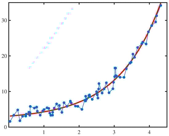
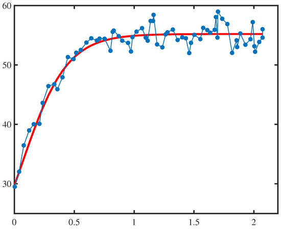
Plotting the fitted exponential growth model (12) and observations in the same graph, and presenting them in Figure 2, we can see that the fitted exponential growth model matches the observations well.

Figure 2. Fitted exponential growth model (12) and observational data of Example 1, which shows a good fit between the fitted exponential growth model and the observational data.

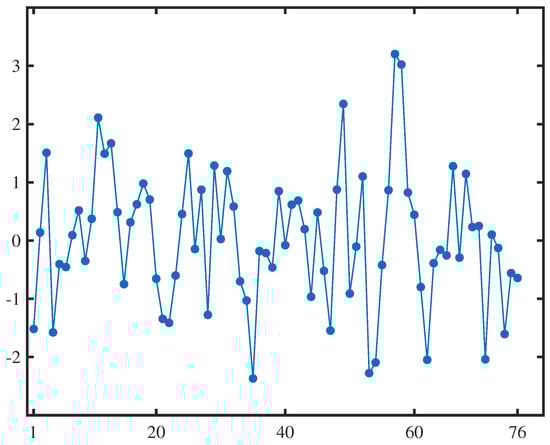
Next, we test the suitability of the estimated uncertain exponential growth model (13) and make predictions based on the new explanatory variables. Using the observations and the estimated parameter values, we can calculate the 76 residuals ${\epsilon }_1,{\epsilon }_2,\cdots ,{\epsilon }_{76}$ of the estimated uncertain exponential growth model (13) according to the following formula:

$${\epsilon }_i=y_i-{\widehat{\beta }}_0-{\widehat{\beta }}_{1}exp\left({\widehat{\beta }}_2{x}_i\right),i=1,2,\cdots ,76,$$

which are shown in Figure 3. Assume that the significance level is set to $\alpha =0.05$, and the critical value calculated at this level is $\alpha \times 76=3.8$. Referring to Equation (8), we can further conclude that the test is

$$\begin{array}{cc}\hfill W=\{(z_1,z_2,\cdots ,z_{76}):& \mathrm{there} \mathrm{are} \mathrm{at} \mathrm{least} 4 \mathrm{of} \mathrm{indexes} i^{\prime }\mathrm{s} \mathrm{with} 1\le i\le 76\hfill \\ \hfill & \mathrm{such} \mathrm{that} z_i<-2.4167 \mathrm{or} z_i>2.4167\}.\hfill \end{array}$$

As depicted in Figure 3, it is evident that only

$${\epsilon }_{57},{\epsilon }_{58}\notin [-2.4167,2.4167].$$

Consequently, we can infer that

$$({\epsilon }_1,{\epsilon }_2,\cdots ,{\epsilon }_{76})\notin W.$$

This strongly supports the conclusion that the estimated uncertain exponential growth model (13) can better adapt to and fit the observation data set depicted in Table 1 and Figure 1.

Figure 3. Residual plot of the estimated uncertain exponential growth model (13) in Example 1.

In addition, if the new explanatory variable is $\widehat{x}=4.5$, then the forecast uncertain variable of the response variable is

$$\begin{array}{c}\hfill \widehat{y}=2.1316+0.9476exp\left(0.8194\widehat{x}\right)+\mathcal{N}(0,1.1965)\sim \mathcal{N}(39.9713,1.1965).\end{array}$$

Then it follows from Equations (9) and (10) that the point forecast value of the response variable $\widehat{y}$ is

$$\widehat{\mu }=E\left[\widehat{y}\right]=39.9713,$$

and the $95\%$ confidence interval is

$$39.9713\pm {\displaystyle \frac{1.1965\times \sqrt{3}}{\pi }}ln{\displaystyle \frac{1+0.95}{1-0.95}},$$

i.e., $39.9713\pm 2.4167$.

Example 2.

When exploring growth patterns in complex environments, another approach is to capture growth trends that gradually accelerate at the beginning of growth, accelerate in the middle of growth, and slow down in the later stages of growth by constructing a logistic growth model, especially under uncertain circumstances such as the process of population evolution or the spread of infectious diseases. The specific logistic growth model is as follows:

$$\begin{array}{c}\hfill y={\beta }_0+{\displaystyle \frac{{\beta }_1}{1+{\beta }_{2}exp\left(-{\beta }_{3}x\right)}}+\epsilon ,\end{array}$$

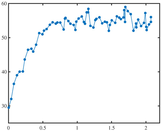
where ${\beta }_0$, ${\beta }_1$, ${\beta }_2$, and ${\beta }_3$ are the parameters to be estimated, and ε is an uncertain disturbance term, which is assumed to follow a normal uncertainty distribution with a mean of 0 and a standard deviation of σ. In addition, for the empirical analysis, we assume that there is a data set containing 68 sets of observations, which are related to the explanatory variables and the response variable, and are presented in the form of Table 2 and Figure 4.

Table 2. Observational data of Example 2.

x	y	x	y	x	y	x	y
0.0030	29.5059	0.6885	54.1126	1.1620	58.4385	1.6830	58.0711
0.0395	32.0362	0.7110	54.4404	1.1915	53.4652	1.6955	54.6119
0.0780	36.4589	0.7530	54.4186	1.2355	52.9707	1.7000	58.9852
0.1230	38.9807	0.8025	52.3946	1.2630	55.1536	1.7355	57.7782
0.1615	40.0327	0.8210	55.5801	1.2780	55.4998	1.7785	56.8902
0.2090	40.0993	0.8295	55.7937	1.3230	55.9606	1.8180	52.0411
0.2360	43.6076	0.8710	54.8597	1.3630	54.2075	1.8555	54.1480
0.2840	46.4421	0.9005	54.0925	1.4020	54.6567	1.8605	53.0196
0.3330	46.7559	0.9490	53.7172	1.4320	54.4987	1.8865	55.2992
0.3590	45.9164	0.9735	52.2714	1.4600	52.0097	1.9290	53.4092
0.4015	47.9307	0.9860	54.6858	1.4750	53.7355	1.9715	54.3374
0.4465	51.3303	1.0200	55.6078	1.5025	55.0737	1.9905	57.2144
0.4935	50.9886	1.0660	56.1994	1.5525	54.3553	2.0040	53.1554
0.5165	52.0612	1.0970	54.6051	1.5765	56.2438	2.0100	52.2278
0.5545	52.5257	1.1130	54.0854	1.6110	55.8744	2.0445	53.8768
0.6015	53.7737	1.1375	57.4118	1.6350	55.4344	2.0725	54.6140
0.6420	54.4962	1.1580	57.4150	1.6725	55.9188	2.0726	56.0243

Figure 4. Observational data of Example 2.

At first, we denote the observations shown in Table 2 and Figure 4 as

$$\begin{array}{c}\hfill (x_i,y_i),i=1,2,\cdots ,68.\end{array}$$

(14)

Then we can obtain 68 real-valued functions with respect to ${\beta }_0$, ${\beta }_1$, ${\beta }_2$, ${\beta }_3$, and $\sigma$ as

$$h_1({\beta }_0,{\beta }_1,{\beta }_2,{\beta }_3,\sigma ),h_2({\beta }_0,{\beta }_1,{\beta }_2,{\beta }_3,\sigma ),\cdots ,h_{68}({\beta }_0,{\beta }_1,{\beta }_2,{\beta }_3,\sigma )$$

by substituting the $(x_i,y_i)$ into

$$h_i({\beta }_0,{\beta }_1,{\beta }_2,{\beta }_3,\sigma )={\displaystyle \frac{{\displaystyle y_i-{\beta }_0-\frac{{\beta }_1}{1+{\beta }_{2}exp\left(-{\beta }_3{x}_i\right)}}}{\sigma }}$$

for $i=1,2,\cdots ,68$. It follows from (5) that the least squares estimations ${\widehat{\beta }}_0$, ${\widehat{\beta }}_1$, ${\widehat{\beta }}_2$, ${\widehat{\beta }}_3$, and $\widehat{\sigma }$ solve the following minimization problem:

$$\begin{array}{cc}\hfill \underset{{\beta }_0,{\beta }_1,{\beta }_2,{\beta }_3,\sigma >0}{min}\sum _{i=1}^{68}& \left({\left(1+exp\left({\displaystyle \frac{-\pi h_i({\beta }_0,{\beta }_1,{\beta }_2,{\beta }_3,\sigma )}{\sqrt{3}}}\right)\right)}^{-1}\right.\hfill \\ \hfill & {\left.-{\displaystyle \frac{1}{68}}\sum _{j=1}^{68}\mathbb{I}(h_j({\beta }_0,{\beta }_1,{\beta }_2,{\beta }_3,\sigma )\le h_i({\beta }_0,{\beta }_1,{\beta }_2,{\beta }_3,\sigma ))\right)}^2\hfill \end{array}$$

which are

$${\widehat{\beta }}_0=11.5185,{\widehat{\beta }}_1=43.6983,{\widehat{\beta }}_2=1.4007,{\widehat{\beta }}_3=5.3150,\widehat{\sigma }=1.6965.$$

Therefore, we obtain a fitted logistic growth model

$$y=11.5185+{\displaystyle \frac{43.6983}{1+1.4007exp\left(-5.3150x\right)}}$$

(15)

and an estimated uncertain logistic growth model

$$y=11.5185+{\displaystyle \frac{43.6983}{1+1.4007exp\left(-5.3150x\right)}}+\mathcal{N}(0,1.6965).$$

(16)

Plotting the fitted logistic growth model (15) and observations in the same graph, and presenting them in Figure 5, we can see that the fitted logistic growth model matches the observations well.

Figure 5. Fitted logistic growth model (15) and observational data of Example 2, which shows a good fit between the fitted exponential growth model and the observational data.

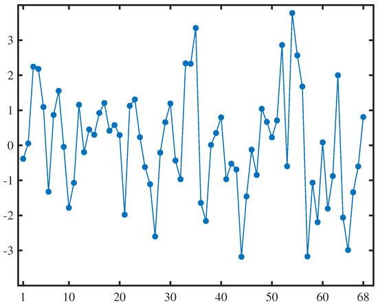
Next, we test the suitability of the estimated uncertain logistic growth model (16) and make predictions based on the new explanatory variables. Using the observations and the estimated parameter values, we can calculate the 68 residuals ${\epsilon }_1,{\epsilon }_2,\cdots ,{\epsilon }_{68}$ of the estimated uncertain logistic growth model (16) according to the following formula:

$${\epsilon }_i=y_i-{\widehat{\beta }}_0-{\displaystyle \frac{{\widehat{\beta }}_1}{1+{\widehat{\beta }}_{2}exp\left(-{\widehat{\beta }}_3{x}_i\right)}},i=1,2,\cdots ,68,$$

which is shown in Figure 6. Assume that the significance level is set to $\alpha =0.05$, and the critical value calculated at this level is $\alpha \times 68=3.4$. Referring to Equation (8), we can further conclude that the test is

$$\begin{array}{cc}\hfill W=\{(z_1,z_2,\cdots ,z_{68}):& \mathrm{there} \mathrm{are} \mathrm{at}\mathrm{least} 4 \mathrm{of} \mathrm{indexes} i^{\prime }\mathrm{s} \mathrm{with} 1\le i\le 68\hfill \\ \hfill & \mathrm{such} \mathrm{that} z_i<-3.4266 \mathrm{or} z_i>3.4266\}.\hfill \end{array}$$

Figure 6. Residual plot of the estimated uncertain logistic growth model (16) in Example 2.

As depicted in Figure 6, it is evident that only

$${\epsilon }_{54}\notin [-3.4266,3.4266].$$

Consequently, we can infer that

$$({\epsilon }_1,{\epsilon }_2,\cdots ,{\epsilon }_{68})\notin W.$$

This strongly supports the conclusion that the estimated uncertain logistic growth model (16) can better adapt to and fit the observation data set depicted in Table 2 and Figure 4.

In addition, if the new explanatory variable is $\widehat{x}=2.1$, then the forecast uncertain variable of the response variable is

$$\begin{array}{c}\hfill \widehat{y}=11.5185+{\displaystyle \frac{43.6983}{1+1.4007exp\left(-5.3150\widehat{x}\right)}}+\mathcal{N}(0,1.6965)\sim \mathcal{N}(55.2160,1.6965).\end{array}$$

Then it follows from Equations (9) and (10) that the point forecast value of the response variable $\widehat{y}$ is

$$\widehat{\mu }=E\left[\widehat{y}\right]=55.2160,$$

and the $95\%$ confidence interval is

$$55.2160\pm {\displaystyle \frac{1.6965\times \sqrt{3}}{\pi }}ln{\displaystyle \frac{1+0.95}{1-0.95}},$$

i.e., $55.2160\pm 3.4266$.

5. Case Study: Forecast of Electrical Power Output

In this section, we will select the data set downloaded from the website of cnblogs.com and accessed on 10 August 2024, which has 9568 data points of a combined cycle power plant during a full load operation for 6 years (2006–2011). The corresponding explanatory variables specifically include the hourly average environmental variable temperature ($x_1$), atmospheric pressure ($x_2$), relative humidity ($x_3$), exhaust vacuum ($x_4$), and the response variable is the full load electrical power output (y) of the plant. Due to the limitation of the amount of data, this paper only intercepts the first 135 data in the data set for modeling analysis, and has realized the forecast of the full load electrical power output. The specific data are shown in Table 3.

Table 3. The first 135 data in the data set of combined cycle power plant during a full load operation, downloaded from the website cnblogs.com.

${\mathit{x}}_1$	${\mathit{x}}_2$	${\mathit{x}}_3$	${\mathit{x}}_4$	y	${\mathit{x}}_1$	${\mathit{x}}_2$	${\mathit{x}}_3$	${\mathit{x}}_4$	y
14.96	41.76	1024.07	73.17	463.26	10.54	34.03	1018.71	74	478.77
25.18	62.96	1020.04	59.08	444.37	27.71	74.34	998.14	71.85	434.2
5.11	39.4	1012.16	92.14	488.56	23.11	68.3	1017.83	86.62	437.91
20.86	57.32	1010.24	76.64	446.48	7.51	41.01	1024.61	97.41	477.61
10.82	37.5	1009.23	96.62	473.9	26.46	74.67	1016.65	84.44	431.65
26.27	59.44	1012.23	58.77	443.67	29.34	74.34	998.58	81.55	430.57
15.89	43.96	1014.02	75.24	467.35	10.32	42.28	1008.82	75.66	481.09
9.48	44.71	1019.12	66.43	478.42	22.74	61.02	1009.56	79.41	445.56
14.64	45	1021.78	41.25	475.98	13.48	39.85	1012.71	58.91	475.74
11.74	43.56	1015.14	70.72	477.5	25.52	69.75	1010.36	90.06	435.12
17.99	43.72	1008.64	75.04	453.02	21.58	67.25	1017.39	79	446.15
20.14	46.93	1014.66	64.22	453.99	27.66	76.86	1001.31	69.47	436.64
24.34	73.5	1011.31	84.15	440.29	26.96	69.45	1013.89	51.47	436.69
25.71	58.59	1012.77	61.83	451.28	12.29	42.18	1016.53	83.13	468.75
26.19	69.34	1009.48	87.59	433.99	15.86	43.02	1012.18	40.33	466.6
21.42	43.79	1015.76	43.08	462.19	13.87	45.08	1024.42	81.69	465.48
18.21	45	1022.86	48.84	467.54	24.09	73.68	1014.93	94.55	441.34
11.04	41.74	1022.6	77.51	477.2	20.45	69.45	1012.53	91.81	441.83
14.45	52.75	1023.97	63.59	459.85	15.07	39.3	1019	63.62	464.7
13.97	38.47	1015.15	55.28	464.3	32.72	69.75	1009.6	49.35	437.99
17.76	42.42	1009.09	66.26	468.27	18.23	58.96	1015.55	69.61	459.12
5.41	40.07	1019.16	64.77	495.24	35.56	68.94	1006.56	38.75	429.69
7.76	42.28	1008.52	83.31	483.8	18.36	51.43	1010.57	90.17	459.8
27.23	63.9	1014.3	47.19	443.61	26.35	64.05	1009.81	81.24	433.63
27.36	48.6	1003.18	54.93	436.06	25.92	60.95	1014.62	48.46	442.84
27.47	70.72	1009.97	74.62	443.25	8.01	41.66	1014.49	76.72	485.13
14.6	39.31	1011.11	72.52	464.16	19.63	52.72	1025.09	51.16	459.12
7.91	39.96	1023.57	88.44	475.52	20.02	67.32	1012.05	76.34	445.31
5.81	35.79	1012.14	92.28	484.41	10.08	40.72	1022.7	67.3	480.8
30.53	65.18	1012.69	41.85	437.89	27.23	66.48	1005.23	52.38	432.55
23.87	63.94	1019.02	44.28	445.11	23.37	63.77	1013.42	76.44	443.86
26.09	58.41	1013.64	64.58	438.86	18.74	59.21	1018.3	91.55	449.77
29.27	66.85	1011.11	63.25	440.98	14.81	43.69	1017.19	71.9	470.71
27.38	74.16	1010.08	78.61	436.65	23.1	51.3	1011.93	80.05	452.17
24.81	63.94	1018.76	44.51	444.26	10.72	41.38	1021.6	63.77	478.29
12.75	44.03	1007.29	89.46	465.86	29.46	71.94	1006.96	62.26	428.54
24.66	63.73	1011.4	74.52	444.37	8.1	40.64	1020.66	89.04	478.27
16.38	47.45	1010.08	88.86	450.69	27.29	62.66	1007.63	58.02	439.58
13.91	39.35	1014.69	75.51	469.02	17.1	49.69	1005.53	81.82	457.32
23.18	51.3	1012.04	78.64	448.86	11.49	44.2	1018.79	91.14	475.51
22.47	47.45	1007.62	76.65	447.14	23.69	65.59	1010.85	88.92	439.66
13.39	44.85	1017.24	80.44	469.18	13.51	40.89	1011.03	84.83	471.99
9.28	41.54	1018.33	79.89	482.8	9.64	39.35	1015.1	91.76	479.81
11.82	42.86	1014.12	88.28	476.7	25.65	78.92	1010.83	86.56	434.78
10.27	40.64	1020.63	84.6	474.99	21.59	61.87	1011.18	57.21	446.58
22.92	63.94	1019.28	42.69	444.22	27.98	58.33	1013.92	54.25	437.76
16	37.87	1020.24	78.41	461.33	18.8	39.72	1001.24	63.8	459.36
21.22	43.43	1010.96	61.07	448.06	18.28	44.71	1016.99	33.71	462.28
13.46	44.71	1014.51	50	474.6	13.55	43.48	1016.08	67.25	464.33
9.39	40.11	1029.14	77.29	473.05	22.99	46.21	1010.71	60.11	444.36
31.07	73.5	1010.58	43.66	432.06	23.94	59.39	1014.32	74.55	438.64
12.82	38.62	1018.71	83.8	467.41	13.74	34.03	1018.69	67.34	470.49
32.57	78.92	1011.6	66.47	430.12	21.3	41.1	1001.86	42.75	455.13
8.11	42.18	1014.82	93.09	473.62	27.54	66.93	1017.06	55.2	450.22
13.92	39.39	1012.94	80.52	471.81	24.81	63.73	1009.34	83.61	440.43
23.04	59.43	1010.23	68.99	442.99	4.97	42.85	1014.02	88.78	482.98
27.31	64.44	1014.65	57.27	442.77	15.22	50.88	1014.19	100.12	460.44
5.91	39.33	1010.18	95.53	491.49	23.88	54.2	1012.81	64.52	444.97
25.26	61.08	1013.68	71.72	447.46	33.01	68.67	1005.2	51.41	433.94
27.97	58.84	1002.25	57.88	446.11	25.98	73.18	1012.28	85.78	439.73
26.08	52.3	1007.03	63.34	442.44	28.18	73.88	1005.89	75.41	434.48
29.01	65.71	1013.61	48.07	446.22	21.67	60.84	1017.93	81.63	442.33
12.18	40.1	1016.67	91.87	471.49	17.67	45.09	1014.26	51.92	457.67
13.76	45.87	1008.89	87.27	463.5	21.37	57.76	1018.8	70.12	454.66
25.5	58.79	1016.02	64.4	440.01	28.69	67.25	1017.71	53.83	432.21
28.26	65.34	1014.56	43.4	441.03	16.61	43.77	1012.25	77.23	457.66
21.39	62.96	1019.49	72.24	452.68	27.91	63.76	1010.27	65.67	435.21
7.26	40.69	1020.43	90.22	474.91

5.1. Uncertain Electrical Power Output Model

At first, we denote the observations shown in Table 3 as

$$x_{i1},x_{i2},x_{i3},x_{i4},y_i,i=1,2,\cdots ,135,$$

(17)

and choose the following uncertain linear regression model:

$$y={\beta }_0+{\beta }_1{x}_1+{\beta }_2{x}_2+{\beta }_3{x}_3+{\beta }_4{x}_4+\epsilon ,$$

(18)

to model the relationship between $x_1,x_2,x_3,x_4$ and y, where ${\beta }_0$, ${\beta }_1$, ${\beta }_2$, ${\beta }_3$, and ${\beta }_4$ are the parameters to be estimated, and $\epsilon$ is an uncertain disturbance term assumed to follow a normal uncertainty distribution with a mean of 0 and a standard deviation of $\sigma$.

By substituting the observations (17) into

$$h_i({\beta }_0,{\beta }_1,{\beta }_2,{\beta }_3,{\beta }_4,\sigma )={\displaystyle \frac{y_i-{\beta }_0-{\sum }_{j=1}^4{\beta }_j{x}_{ij}}{\sigma }}$$

for $i=1,2,\cdots ,135$, we can obtain 135 real-valued functions with respect to ${\beta }_0$, ${\beta }_1$, ${\beta }_2$, ${\beta }_3$, ${\beta }_4$ and $\sigma$ as

$$h_1({\beta }_0,{\beta }_1,{\beta }_2,{\beta }_3,{\beta }_4,\sigma ),h_2({\beta }_0,{\beta }_1,{\beta }_2,{\beta }_3,{\beta }_4,\sigma ),\cdots ,h_{76}({\beta }_0,{\beta }_1,{\beta }_2,{\beta }_3,{\beta }_4,\sigma ).$$

Then it follows from (5) that the least squares estimations ${\widehat{\beta }}_0$, ${\widehat{\beta }}_1$, ${\widehat{\beta }}_2$, ${\widehat{\beta }}_3$, ${\widehat{\beta }}_4$, and $\widehat{\sigma }$ solve the following minimization problem:

$$\begin{array}{cc}\hfill \underset{{\beta }_0,{\beta }_1,{\beta }_2,{\beta }_3,{\beta }_4,\sigma >0}{min}\sum _{i=1}^{135}& \left({\left(1+exp\left({\displaystyle \frac{-\pi h_i({\beta }_0,{\beta }_1,{\beta }_2,{\beta }_3,{\beta }_4,\sigma )}{\sqrt{3}}}\right)\right)}^{-1}\right.\hfill \\ \hfill & {\left.-{\displaystyle \frac{1}{135}}\sum _{j=1}^{135}\mathbb{I}(h_j({\beta }_0,{\beta }_1,{\beta }_2,{\beta }_3,{\beta }_4,\sigma )\le h_i({\beta }_0,{\beta }_1,{\beta }_2,{\beta }_3,{\beta }_4,\sigma ))\right)}^2,\hfill \end{array}$$

which are

$${\widehat{\beta }}_0=515.9451,{\widehat{\beta }}_1=-2.5699,{\widehat{\beta }}_2=-0.0763,{\widehat{\beta }}_3=0.0166,{\widehat{\beta }}_4=-0.3275,\widehat{\sigma }=5.4886.$$

Therefore, we obtain a fitted electrical power output model

$$y=515.9451-2.5699x_1-0.0763x_2+0.0166x_3-0.3275x_4,$$

and an estimated uncertain electrical power output model

$$y=515.9451-2.5699x_1-0.0763x_2+0.0166x_3-0.3275x_4+\mathcal{N}(0,5.4886).$$

(19)

5.2. Uncertain Hypothesis Test and Electrical Power Output Forecast

Next, we test the suitability of the estimated uncertain electrical power output model (19) and forecast the electrical power output based on the new explanatory variables. Using the observations and the estimated parameter values, we can calculate the 135 residuals ${\epsilon }_1,{\epsilon }_2,\cdots ,{\epsilon }_{135}$ of the estimated uncertain electrical power output model (19) according to the following formula:

$${\epsilon }_i=y_i-{\widehat{\beta }}_0-\sum _{j=1}^4{\widehat{\beta }}_j{x}_{ij},i=1,2,\cdots ,135,$$

which is shown in Figure 7. Assume that the significance level is set to $\alpha =0.05$, and the critical value calculated at this level is $\alpha \times 135=6.75$. Referring to Equation (8), we can further conclude that the test is

$$\begin{array}{cc}\hfill W=\{(z_1,z_2,\cdots ,z_{135}):& \mathrm{there} \mathrm{are} \mathrm{at} \mathrm{least} 7 \mathrm{of} \mathrm{indexes} i^{\prime }\mathrm{s} \mathrm{with} 1\le i\le 135\hfill \\ \hfill & \mathrm{such} \mathrm{that} z_i<-11.0860 \mathrm{or} z_i>11.0860\}.\hfill \end{array}$$

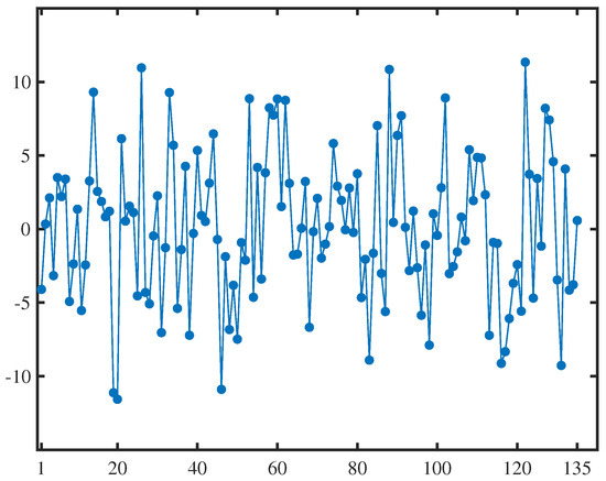
Figure 7. Residual plot of the estimated uncertain electrical power output model (19).

As depicted in Figure 7, it is evident that only

$${\epsilon }_{19},{\epsilon }_{20},{\epsilon }_{122}\notin [-11.0860,11.0860].$$

Consequently, we can infer that

$$({\epsilon }_1,{\epsilon }_2,\cdots ,{\epsilon }_{135})\notin W.$$

This strongly supports the conclusion that the estimated uncertain electrical power output model (19) can better adapt to and fit the observation data set depicted in Table 3.

In addition, if the new explanatory variable is

$$({\widehat{x}}_1,{\widehat{x}}_2,{\widehat{x}}_3,{\widehat{x}}_4)=(20.97,47.43,1007.64,71.18),$$

then the forecast uncertain variable of the electrical power output is

$$\begin{array}{cc}\hfill \widehat{y}& =515.9451-2.5699{\widehat{x}}_1-0.0763{\widehat{x}}_2+0.0166{\widehat{x}}_3-0.3275{\widehat{x}}_4+\mathcal{N}(0,5.4886)\hfill \\ \hfill & \sim \mathcal{N}(451.8605,5.4886).\hfill \end{array}$$

Then it follows from Equations (9) and (10) that the point forecast value of the electrical power output $\widehat{y}$ is

$$\widehat{\mu }=E\left[\widehat{y}\right]=451.8605,$$

and the $95\%$ confidence interval is

$$451.8605\pm {\displaystyle \frac{5.4886\times \sqrt{3}}{\pi }}ln{\displaystyle \frac{1+0.95}{1-0.95}},$$

i.e., $451.8605\pm 11.0860$.

6. Conclusions

For the sake of overcoming the limitation of the traditional least squares method in dealing with uncertain regression models, this paper creatively combined the least squares principle with the mathematical properties of the normal uncertainty distribution, and proposed a least squares estimation method for unknown parameters and disturbance term of uncertain regression models. In order to handle the calculation problem of related estimators, this paper also designed a numerical algorithm to solve the specific parameter values under this estimation method. Finally, through two numerical examples and empirical research on electrical power output forecast, this paper fully illustrated the effectiveness of the proposed least squares estimation method.

The greatest contribution of this paper is the least squares estimation of an uncertain regression model based on the mathematical properties of the normal uncertainty distribution and the observed data. The shortcoming of this paper is that it is difficult to solve the corresponding estimators analytically. This paper only designed a simple numerical algorithm without considering the speed and convergence of numerical solutions. Future research content can be driven from this perspective, and more extensive empirical research can also be conducted based on the proposed method.

References

- Galton, F. Family likeness in stature. Proc. R. Soc. Lond. 1886, 40, 42–73. [Google Scholar]
- Berkson, J. Application of the logistic function to bio-assay. J. Am. Stat. Assoc. 1944, 39, 357–365. [Google Scholar]
- Hoerl, A.; Kennard, R. Ridge regression: Biased estimation for nonorthogonal problems. Technometrics 1970, 12, 55–67. [Google Scholar] [CrossRef]
- Tibshirani, R. Regression shrinkage and selection via the lasso. J. R. Stat. Soc. Ser. B Stat. Methodol. 1996, 58, 267–288. [Google Scholar] [CrossRef]
- Zou, H.; Hastie, T. Regularization and variable selection via the elastic net. J. R. Stat. Soc. Ser. B Stat. Methodol. 2005, 67, 301–320. [Google Scholar] [CrossRef]
- Freund, R.; Wilson, W.; Sa, P. Regression Analysis; Elsevier: Amsterdam, The Netherlands, 2006. [Google Scholar]
- Sen, A.; Srivastava, M. Regression Analysis: Theory, Methods, Applications; Springer Science & Business Media: Berlin/Heidelberg, Germany, 2012. [Google Scholar]
- Chatterjee, S.; Simonoff, J. Handbook of Regression Analysis; John Wiley & Sons: Hoboken, NJ, USA, 2013. [Google Scholar]
- Liu, B. Uncertainty Theory, 2nd ed.; Springer: Berlin, Germany, 2007. [Google Scholar]
- Liu, B. Some research problems in uncertainty theory. J. Uncertain Syst. 2009, 3, 3–10. [Google Scholar]
- Yao, K.; Liu, B. Uncertain regression analysis: An approach for imprecise observations. Soft Comput. 2018, 22, 5579–5582. [Google Scholar] [CrossRef]
- Ye, T.; Liu, Y.H. Multivariate uncertain regression model with imprecise observations. J. Ambient. Intell. Humaniz. Comput. 2020, 11, 4941–4950. [Google Scholar] [CrossRef]
- Chen, D. Uncertain regression model with autoregressive time series errors. Soft Comput. 2021, 25, 14549–14559. [Google Scholar] [CrossRef]
- Chen, D. Uncertain regression model with moving average time series errors. Commun. Stat. Theory Methods 2023, 52, 7632–7646. [Google Scholar] [CrossRef]
- Jiang, B.; Ye, T. Uncertain panel regression analysis with application to the impact of urbanization on electricity intensity. J. Ambient. Intell. Humaniz. Comput. 2023, 14, 13017–13029. [Google Scholar] [CrossRef]
- Ding, J.; Zhang, Z. Statistical inference on uncertain nonparametric regression model. Fuzzy Optim. Decis. Mak. 2021, 20, 451–469. [Google Scholar] [CrossRef]
- Liu, Z.; Yang, Y. Least absolute deviations estimation for uncertain regression with imprecise observations. Fuzzy Optim. Decis. Mak. 2020, 19, 33–52. [Google Scholar] [CrossRef]
- Lio, W.; Liu, B. Uncertain maximum likelihood estimation with application to uncertain regression analysis. Soft Comput. 2020, 24, 9351–9360. [Google Scholar] [CrossRef]
- Chen, D. Tukey’s biweight estimation for uncertain regression model with imprecise observations. Soft Comput. 2020, 24, 16803–16809. [Google Scholar] [CrossRef]
- Liu, Y. Moment estimation for uncertain regression model with application to factors analysis of grain yield. Commun. Stat. Simul. Comput. 2022, 1–11. [Google Scholar] [CrossRef]
- Xie, W.; Wu, J.; Sheng, Y. Uncertain regression model based on Huber loss function. J. Intell. Fuzzy Syst. 2023, 45, 1169–1178. [Google Scholar] [CrossRef]
- Lio, W.; Liu, B. Residual and confidence interval for uncertain regression model with imprecise observations. J. Intell. Fuzzy Syst. 2018, 35, 2573–2583. [Google Scholar] [CrossRef]
- Liu, Y.; Liu, B. A modified uncertain maximum likelihood estimation with applications in uncertain statistics. Commun. Stat. Theory Methods 2024, 53, 6649–6670. [Google Scholar] [CrossRef]
- Liu, Y.; Liu, B. Estimation of uncertainty distribution function by the principle of least squares. Commun. Stat. Theory Methods 2023, 1–18. [Google Scholar] [CrossRef]
- Liu, Z. Uncertain growth model for the cumulative number of COVID-19 infections in China. Fuzzy Optim. Decis. Mak. 2021, 20, 229–242. [Google Scholar] [CrossRef]
- Yang, L. Analysis of death toll from COVID-19 in China with uncertain time series and uncertain regression analysis. J. Uncertain Syst. 2022, 15, 2243007. [Google Scholar] [CrossRef]
- Ding, C.; Ye, T. Uncertain logistic growth model for confirmed COVID-19 cases in Brazil. J. Uncertain Syst. 2022, 15, 2243008. [Google Scholar] [CrossRef]
- Li, H.; Yang, X.; Ni, Y. Uncertain yield-density regression model with application to parsnips. Int. J. Gen. Syst. 2023, 52, 777–801. [Google Scholar] [CrossRef]
- Liu, Y. Analysis of China’s population with uncertain statistics. J. Uncertain Syst. 2022, 15, 2243001. [Google Scholar] [CrossRef]
- Gao, C.; Liu, Y.; Ning, Y.; Gao, H.; Hu, B. Analysis of the number of students in general colleges and universities in China with uncertain statistics. Soft Comput. 2023. [Google Scholar] [CrossRef]
- Chen, D.; Yang, X. Maximum likelihood estimation for uncertain autoregressive model with application to carbon dioxide emissions. J. Intell. Fuzzy Syst. 2021, 40, 1391–1399. [Google Scholar] [CrossRef]
- Ye, T.; Liu, B. Uncertain significance test for regression coefficients with application to regional economic analysis. Commun. Stat.-Theory Methods 2023, 52, 7271–7288. [Google Scholar] [CrossRef]
- Jia, Y.; Tang, H. Modeling China’s per capita disposable income by uncertain statistics. J. Uncertain Syst. 2023. [Google Scholar] [CrossRef]
- Ye, T.; Liu, B. Uncertain hypothesis test with application to uncertain regression analysis. Fuzzy Optim. Decis. Mak. 2022, 21, 157–174. [Google Scholar]
Disclaimer/Publisher’s Note: The statements, opinions and data contained in all publications are solely those of the individual author(s) and contributor(s) and not of MDPI and/or the editor(s). MDPI and/or the editor(s) disclaim responsibility for any injury to people or property resulting from any ideas, methods, instructions or products referred to in the content. |
© 2024 by the authors. Licensee MDPI, Basel, Switzerland. This article is an open access article distributed under the terms and conditions of the Creative Commons Attribution (CC BY) license (https://creativecommons.org/licenses/by/4.0/).