A New Generalization of the Inverse Generalized Weibull Distribution with Different Methods of Estimation and Applications in Medicine and Engineering

Abstract

Limitations inherent to existing statistical distributions in capturing the complexities of real-world data often necessitate the development of novel models. This paper introduces the new exponential generalized inverse generalized Weibull (NEGIGW) distribution. The NEGIGW distribution boasts significant flexibility with symmetrical and asymmetrical shapes, allowing its hazard rate function to be adapted to many failure patterns observed in various fields such as medicine, biology, and engineering. Some statistical properties of the NEGIGW distribution, such as moments, quantile function, and Renyi entropy, are studied. Three methods are used for parameter estimation, including maximum likelihood, maximum product of spacing, and percentile methods. The performance of the estimation methods is evaluated via Monte Carlo simulations. The NEGIGW distribution excels in its ability to fit real-world data accurately. Five medical and engineering datasets are applied to demonstrate the superior fit of NEGIGW distribution compared to competing models. This compelling evidence suggests that the NEGIGW distribution is promising for lifetime data analysis and reliability assessments across different disciplines.

1. Introduction

Probability distributions are essential for data modeling in many disciplines, including economics, engineering, biology, business, and the medical sciences. Therefore, several extended distributions have been proposed to enhance the functionality and adaptability of the density and hazard rate functions to model data diversity. The techniques for extending distributions include compounding, adding parameters, composing, and transforming. For instance, the beta-generated method by [1], the Kumaraswamy-generated method by [2], and the transformed-transformer approach by [3] among others.

A new lifetime family named the exponential-X (NLTE-X) was developed by [4]. This family is based on the T-X generator with $T\sim Exp\left(1\right)$ and $W\left(F\left(x\right)\right)=-log\left\{{\displaystyle \frac{1-F\left(x\right)}{e^{\theta F\left(x\right)}}}\right\}$. The cumulative distribution function (CDF) and probability density function (PDF) of NLTE-X are given by:

$$G(x;\theta ,\xi )=1-\left\{{\displaystyle \frac{1-F(x;\Theta )}{e^{\theta F(x;\Theta )}}}\right\};\theta >0,x>0,$$

(1)

$$g(x;\theta ,\xi )=f\left(x\right){\displaystyle \frac{\{1+\theta \overline{F}(x;\Theta )\}}{e^{\theta F(x;\Theta )}}};\theta >0,x>0,$$

(2)

where $\Theta$ is the vector of distribution parameters, and $\theta$ is a parameter of the NLTE-X family. Various distributions were generated from the NLTE-X family, such as the exponential Fréchet distribution [5], exponential inverted Topp–Leone distribution [6], and exponential-X power family of distribution [7].

Inverted distributions have attracted many researchers’ interest. Studies have shown that inverted distributions have more flexible density and hazard function structures than non-inverted ones. In addition, the applications of inverted distributions are significant in various domains, including the biological sciences, life test problems, chemical data, and medicine. For example, In reliability analysis, the inverse Weibull distribution (IW) can accurately model the lifetime of various systems [8,9]. The inverted Kumaraswamy distribution introduced by [10] was applied to precipitation, repairable items, and vinyl chloride data. Moreover, the inverted Topp–Leone distribution was applied to the failure times of Aarset data [11].

Recently, some generalizations of the inverse distributions were studied in the literature. These include the Kumaraswamy–inverse Weibull distribution proposed by [12], the Kumaraswamy inverse exponential distribution developed by [13], the alpha power inverse Rayleigh distribution developed by [14], the exponentiated inverse Rayleigh distribution introduced by [15], and the Weibull inverted exponential distribution by [16]. The Marshall–Olkin alpha power inverse Weibull distribution by [17], the alpha-power exponentiated inverse Rayleigh distribution proposed by [18], the odd Weibull inverse Topp–Leone distribution proposed by [19], the odds generalized exponential-inverse Weibull distribution proposed by [20], the generalized inverted Kumaraswamy distribution introduced by [21], the Kumaraswamy generalized inverse Lomax distribution developed by [22], and the inverse Weibull generator of distribution proposed by [23].

Moreover, a new generalization of both the IW and generalized inverse Weibull distribution (GIW) [24], named the generalized inverse generalized Weibull (GIGW), with CDF and PDF is given by

$$F_{GIGW}\left(x\right)=1-{\left(1-e^{-\gamma {(\lambda /x)}^{\beta }}\right)}^{\alpha };x>0,\gamma ,\lambda ,\alpha ,\beta >0,$$

(3)

$$f_{GIGW}\left(x\right)=\alpha {\lambda }^{\beta }{\beta }^{\beta }\gamma x^{-(\beta +1)}{e}^{-\gamma {(\lambda /x)}^{\beta }}{(1-e^{-\gamma {(\lambda /x)}^{\beta }})}^{\alpha -1};x>0,$$

(4)

where $\lambda$ is the scale parameter and $\alpha ,\beta ,$ and $\gamma$ are the shape parameters. Some of the properties of this distribution are studied by [25]. In addition, ref. [26] has obtained some estimators of the parameter of GIGW using maximum likelihood and the Bayesian estimation methods.

The main purpose of this article is to introduce a new generalization of the IW and inverse generalized Weibull based on the NLTE-X family of distributions called the new exponential generalized inverse generalized Weibull (NEGIGW). The significance of the NEGIGW distribution and its desirable characteristics include the following:

• The NEGIGW will improve the features and adaptability of the density and hazard rate functions, accurately capturing the behavior of several real-world phenomena. The hazard rate function of the NEGIGW exhibits a wide range of forms, including decreasing, bath-tab and upside-down bath-tab, and reversed J-shape. The density can take symmetrical and asymmetrical shapes. This will enable NEGIGW to fit a wide range of data from the engineering, medicine, and reliability fields.
• The NEGIGW introduces new generalizations of the IW, inverse generalized Weibull (IGW), and GIGW distributions by adding new parameters, thus increasing their flexibility and improving their ability to characterize tail shapes more accurately as observed from the different shapes of the NEGIGW density and hazard functions. Therefore, this generalization will help IW, IGW, and GIGW’s inability to fit real-world data such as the lifetime of some cancer data that showed a non-monotone failure rate when it attained a maximum after a finite period and then decreased gradually.
• The CDF and hazard rate functions, moments, and entropy of the NEGIGW are in closed forms, which are useful in analyzing complete and censored data.
• The applications of five medical and engineering data illustrate that the NEGIGW performs better than other competing lifetime models when modeling bladder cancer, failure of the engine’s turbocharger, fatigue Fracture of Kevlar 373/epoxy and failure and service times of aircraft windshield data.

Additionally, this study extends its investigation by evaluating the performance of various estimation methods for the parameters of the NEGIGW distribution. Three prominent techniques are compared: maximum likelihood (ML), maximum product of spacing (MPS), and percentile (PC) methods. A simulation study is conducted to assess the effectiveness of these estimators across a range of sample sizes and parameter values. The statistical analysis of the simulation results will provide valuable insights into the behavior and accuracy of each method under different conditions. Moreover, the applicability of the NEGIGW distribution is explored by demonstrating its superior fit to five practical applications compared to competing distributions. This comparative analysis strengthens the case for the NEGIGW distribution as a versatile tool for modeling real-world phenomena.

This article is structured as follows: Section 2 presents the NEGIGW with some graphical representations. We derived some of the NEGIGW properties in Section 3. In Section 4, three methods of estimation are used to estimate the parameter of the NEGIGW. Section 5, demonstrates extensive simulation studies to examine the performance of the various estimators. In Section 6, five applications in various domains are investigated to examine the NEGIGW’s effectiveness. Finally, some concluding remarks are made in Section 7.

2. New Exponential Generalized Inverse Generalized Weibull Distribution

The CDF and PDF of the NEGIGW can be derived by substituting (3) and (4) in (1) and (2) as follows

$$G\left(x\right)=1-{\displaystyle \frac{{\left(1-e^{-\gamma {(\lambda /x)}^{\beta }}\right)}^{\alpha }}{e^{\theta \left(1-{\left(1-e^{-\gamma {(\lambda /x)}^{\beta }}\right)}^{\alpha }\right)}}},x>0,\theta ,\gamma ,\alpha ,\lambda ,\beta >0,$$

(5)

$$\begin{array}{c}\hfill g\left(x\right)=\alpha {\lambda }^{\beta }\beta \gamma x^{-(\beta +1)}{e}^{-\gamma {(\lambda /x)}^{\beta }}{(1-e^{-\gamma {(\lambda /x)}^{\beta }})}^{\alpha -1}{\displaystyle \frac{\left[1+\theta {\left(1-e^{-\gamma {(\lambda /x)}^{\beta }}\right)}^{\alpha }\right]}{e^{\theta \left(1-{\left(1-e^{-\gamma {(\lambda /x)}^{\beta }}\right)}^{\alpha }\right)}}}.\end{array}$$

(6)

The survival $S\left(x\right)$ function is expressed as

$$S\left(x\right)={\displaystyle \frac{{\left(1-e^{-\gamma {(\lambda /x)}^{\beta }}\right)}^{\alpha }}{e^{\theta (1-{\left(1-e^{-\gamma {(\lambda /x)}^{\beta }}\right)}^{\alpha })}}}.$$

(7)

The hazard rate function (HF), which is frequently utilized in lifetime modeling as it indicates the likelihood of failure, is defined as

$$\begin{array}{c}\hfill HF=\alpha {\lambda }^{\beta }\beta \gamma x^{-(\beta +1)}{e}^{-\gamma {(\lambda /x)}^{\beta }}{\displaystyle \frac{\left[1+\theta {\left(1-e^{-\gamma {(\lambda /x)}^{\beta }}\right)}^{\alpha }\right]}{(1-e^{-\gamma {(\lambda /x)}^{\beta }})}}.\end{array}$$

(8)

The NEGIGW distribution’s versatility in representing real-world data is evident in its ability to generate a wide range of shapes for its PDF and HF. The density plots in Figure 1 show decreasing, right-skewed, left-skewed, and symmetrical shapes, indicating its ability to fit complicated data. The HF plots of the NEGIGW in Figure 2 exhibit diverse asymmetrical forms such as unimodal, decreasing, and upside-down bathtubs, allowing for modeling failure rates that change over time. This flexibility of NEGIGW makes it a powerful tool for researchers and analysts. Researchers can tailor the NEGIGW to capture the underlying patterns of diverse real-world phenomena. This capability can lead to more precise modeling and improved decision-making across various fields, from finance and engineering to ecology and medicine.

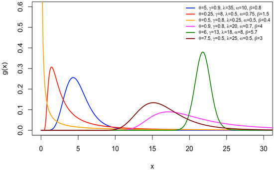
Figure 1. The NEGIGW density plots.

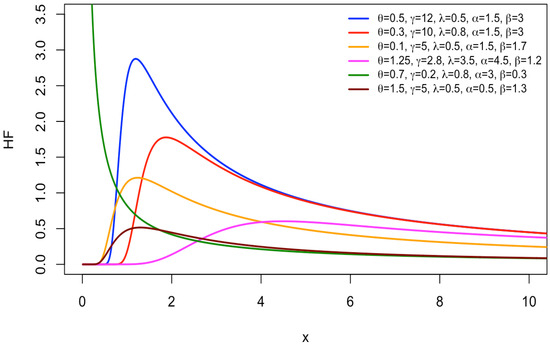
Figure 2. The NEGIGW HF’s plots.

2.1. Linear Representation for the Density of NEGIGW

A linear representation of the PDF of NEGIGW has been developed using mathematical expansions. The derivation begins with the binomial theorem, given by

$${(1-x)}^n=\sum _{i=0}^n{(-1)}^i\left({\displaystyle \genfrac{}{}{0pt}{}{n}{i}}\right)x^i.$$

(9)

By applying (9), the PDF of NEGIGW will become

$$\begin{array}{c}\hfill g\left(x\right)=\sum _{v_1=0}^1\alpha {\lambda }^{\beta }\beta \gamma {\theta }_1^v\left({\displaystyle \genfrac{}{}{0pt}{}{1}{v_1}}\right)x^{-(\beta +1)}{e}^{-\gamma {(\lambda /x)}^{\beta }}{(1-e^{-\gamma {(\lambda /x)}^{\beta }})}^{\alpha +\alpha v_1-1}{e}^{-\theta \left[1-{\left(1-e^{-\gamma {(\lambda /x)}^{\beta }}\right)}^{\alpha }\right]}\end{array}$$

The exponential expansion with a positive exponent is given by

$$e^x=\sum _{i=0}^{\infty }{\displaystyle \frac{x^i}{i!}}.$$

(10)

Then, the PDF will be

$$\begin{array}{c}\hfill g\left(x\right)=\sum _{v_1=0}^1\sum _{v_2=0}^{\infty }\left({\displaystyle \genfrac{}{}{0pt}{}{1}{v_1}}\right){\displaystyle \frac{\alpha {\lambda }^{\beta }\beta \gamma {\theta }^{v_1+v_2}{e}^{-\theta }}{v_2!}}{x}^{-(\beta +1)}{e}^{-\gamma {(\lambda /x)}^{\beta }}{(1-e^{-\gamma {(\lambda /x)}^{\beta }})}^{\alpha (v_1+v_2+1)-1}\end{array}$$

Applying (9) again, the PDF of NEGIGW will reduced to

$$\begin{array}{c}\hfill g\left(x\right)=\sum _{v_3=0}^{\infty }{\eta }_{v_3}{\lambda }^{\beta }\beta \gamma x^{-(\beta +1)}{e}^{-(v_3+1)\gamma {(\lambda /x)}^{\beta }},\end{array}$$

(11)

where

$$\begin{array}{c}\hfill {\eta }_{v_3}=\sum _{v_1=0}^1\sum _{v_2=0}^{\infty }\left({\displaystyle \genfrac{}{}{0pt}{}{1}{v_1}}\right)\left({\displaystyle \genfrac{}{}{0pt}{}{\alpha (v_1+v_2+1)-1}{v_3}}\right){\displaystyle \frac{{(-1)}^{v_3}\alpha {\theta }^{v_1+v_2}{e}^{-\theta }}{v_2!}}.\end{array}$$

(12)

2.2. Some Special Cases of NEGIGW

Special cases of NEGIGW can be obtained as follows:

• When $\gamma =1$ and $\alpha =1$, the NEGIGW reduces to the exponential Fréchet distribution with parameters $\beta$, $\theta$, and $\lambda$ presented in [5].
• When $\beta =1$ and $\gamma =1$, the NEGIGW reduces to the exponential generalized inverse exponential distribution with parameters $\alpha$, $\theta$, and $\lambda$; (not been previously studied).
• When $\beta =2$ and $\alpha =1$, the NEGIGW reduces to the exponential generalized inverse Rayleigh distribution with parameters $\gamma$, $\theta$, and $\lambda$; (not been previously studied).

3. Properties of the NEGIGW

In this section, some characteristic properties of the NEGIGW are derived.

3.1. Quantile Function

The uth quantile function $(0<u<1)$ of $X\sim$ NEGIGW can be derived by inverting (5) and solving the non-linear equation by the Lambert function $W[.]$.

$$x_u=\lambda {\left\{-{\displaystyle \frac{1}{\gamma }}log\left\{1-{\left\{{\displaystyle \frac{W\left(\theta e^{\theta }(1-u)\right)}{\theta }}\right\}}^{{\displaystyle \frac{1}{\alpha }}}\right\}\right\}}^{{\displaystyle \frac{-1}{\beta }}},0\le u\le 1.$$

(13)

The median of the NEGIGW can be obtained by substituting $u=0.5$ into Equation (13).

$$Median\left(x\right)=\lambda {\left\{-{\displaystyle \frac{1}{\gamma }}log\left\{1-{\left\{{\displaystyle \frac{W\left(\theta e^{\theta }\left(0.5\right)\right)}{\theta }}\right\}}^{{\displaystyle \frac{1}{\alpha }}}\right\}\right\}}^{{\displaystyle \frac{-1}{\beta }}}.$$

(14)

3.2. Moment

The $rth$ moment of $X\sim$ NEGIGW is obtained as follows

$$\begin{array}{c}\hfill \begin{array}{cc}\hfill {\mu }_r& =E\left(x^r\right)={\int }_0^{\infty }{x}^{r}g\left(x\right)dx\hfill \\ & =\sum _{v_3=0}^{\infty }{\eta }_{v_3}{\lambda }^{\beta }\beta \gamma {\int }_0^{\infty }{x}^r{x}^{-(\beta +1)}{e}^{-(v_3+1)\gamma {(\lambda /x)}^{\beta }}dx.\hfill \end{array}\end{array}$$

(15)

By substituting $y=(v_3+1)\gamma {(\lambda /x)}^{\beta }$, therefore, the $rth$ moment can be defined as

$$\begin{array}{c}\hfill {\mu }_r=\sum _{v_3=0}^{\infty }{\eta }_{v_3}{\lambda }^r{\gamma }^{\frac{r}{\beta }}{(v_3+1)}^{\frac{r}{\beta }-1}\Gamma \left(1-{\displaystyle \frac{r}{\beta }}\right),\beta >r,\end{array}$$

(16)

where ${\eta }_{v_3}$ is given by (12)

3.3. Moment Generating Function

The moment-generating function (MGF) of the NEGIGW is defined as

$$\begin{array}{c}\hfill M_X\left(t\right)=E\left(e^{tx}\right)=\sum _{r=0}^{\infty }{\displaystyle \frac{t^r}{r!}}{\mu }_r.\end{array}$$

(17)

Therefore, substituting (16) into (17), the MGF is obtained as

$$\begin{array}{c}\hfill M_X\left(t\right)=\sum _{r=0}^{\infty }\frac{t^r}{r!}\sum _{v_3=0}^{\infty }{\eta }_{v_3}{\lambda }^r{\gamma }^{\frac{r}{\beta }}{(v_3+1)}^{{\displaystyle \frac{r}{\beta }}-1}\Gamma \left(1-{\displaystyle \frac{r}{\beta }}\right),\beta >r,\end{array}$$

(18)

where ${\eta }_{v_3}$ is given by (12).

3.4. Characteristic Function

The NEGIGW characteristic function is obtained as

$$\begin{array}{c}\hfill {\varphi }_x\left(t\right)=E\left(e^{itx}\right)=\sum _{r=0}^{\infty }\frac{{\left(it\right)}^r}{r!}\sum _{v_3=0}^{\infty }{\eta }_{v_3}{\lambda }^r{\gamma }^{\frac{r}{\beta }}{(v_3+1)}^{\frac{r}{\beta }-1}\Gamma \left(1-\frac{r}{\beta }\right),\beta >r,\end{array}$$

(19)

where ${\eta }_s$ is given by (12).

3.5. Rényi Entropy

The Rényi entropy can be used to determine the uncertainty measurement of the random variable X. When the Rényi entropy value is high, the data’s uncertainty level increases. According to [27], the Rényi entropy, $RE\left(\mathsf{\delta }\right)$, can be expressed as

$$RE\left(\mathsf{\delta }\right)={\displaystyle \frac{1}{1-\mathsf{\delta }}}log\left[{\int }_{-\infty }^{\infty }{\left[g\left(x\right)\right]}^{\mathsf{\delta }}dx\right]$$

(20)

By substituting $g\left(x\right)$ given in (6) into the (20) and applying the expansions (10) and (9). $RE\left(\mathsf{\delta }\right)$ is presented as

$$\begin{array}{c}\hfill {\left[g\left(x\right)\right]}^{\mathsf{\delta }}=\sum _{v_3=0}^{\infty }{\eta }_{v_3}^{*}{\beta }^{\mathsf{\delta }}{\gamma }^{\mathsf{\delta }}{\lambda }^{\mathsf{\delta }\beta }{x}^{-\mathsf{\delta }(\beta +1)}{e}^{-\gamma (\mathsf{\delta }+v_3){(\lambda /x)}^{\beta }},\end{array}$$

(21)

where

$$\begin{array}{c}\hfill {\eta }_{v_3}^{*}=\sum _{v_1=0}^{\mathsf{\delta }}\sum _{v_2=0}^{\infty }\left({\displaystyle \genfrac{}{}{0pt}{}{\mathsf{\delta }}{v_1}}\right)\left({\displaystyle \genfrac{}{}{0pt}{}{\alpha (v_1+v_2+\mathsf{\delta })-\mathsf{\delta }}{v_3}}\right){\displaystyle \frac{{(-1)}^{v_3}{\alpha }^{\mathsf{\delta }}{\mathsf{\delta }}^{v_2}{\theta }^{v_1+v_2}{e}^{-\theta \mathsf{\delta }}}{v_2!}}.\end{array}$$

(22)

By replacing (21) in (20), and calculating the integral, the Rényi entropy of the NEGIGW can be derived as

$$\begin{array}{c}\hfill RE\left(\mathsf{\delta }\right)={\displaystyle \frac{1}{1-\mathsf{\delta }}}log\left[\sum _{v_3=0}^{\infty }{\eta }_{v_3}^{*}{\displaystyle \frac{{\beta }^{(\delta -1)}{\lambda }^{(1-\delta )}}{{(\delta +v_3)}^{\frac{1}{\beta }[\delta (\beta +1)-1]}{\gamma }^{\frac{1}{\beta }(\delta -1)}}}\Gamma \left({\displaystyle \frac{1}{\beta }}[\delta (\beta +1)-1]\right)\right].\end{array}$$

(23)

3.6. Order Statistics

Let $X_{i:n}$ denote the ith order statistics for NEGIGW’s random sample (RS) $X_1,X_2,\cdots ,X_n$. Therefore, the ith order statistics PDF, $f_{i:n}\left(x\right)$, is presented as

$$f_{i:n}\left(x\right)={\displaystyle \frac{n!}{(i-1)!(n-i)!}}f\left(x\right){\left[F\left(x\right)\right]}^{i-1}{\left[1-F\left(x\right)\right]}^{n-i}.$$

(24)

Using (9), the PDF of $X_{i:n}$ becomes

$$f_{i:n}\left(x\right)=\sum _{k=0}^n{\displaystyle \frac{{(-1)}^{k}n!}{(i-1)!(n-i)!}}\left({\displaystyle \genfrac{}{}{0pt}{}{n}{k}}\right)f\left(x\right){\left[F\left(x\right)\right]}^{k+i-1}.$$

(25)

Substituting (5) into (25), the PDF of $X_{i:n}$

$$\begin{array}{c}\hfill f_{i:n}\left(x\right)=\sum _{k=0}^n{\displaystyle \frac{{(-1)}^{k}n!}{(i-1)!(n-i)!}}\left({\displaystyle \genfrac{}{}{0pt}{}{n}{k}}\right)f\left(x\right){\left[1-{\displaystyle \frac{{(1-e^{-\gamma {(\lambda /x)}^{\beta }})}^{\alpha }}{e^{\theta \left(1-{\left(1-e^{-\gamma {(\lambda /x)}^{\beta }}\right)}^{\alpha }\right)}}}\right]}^{k+i-1},\end{array}$$

(26)

where $f\left(x\right)$ given by (6).

4. Estimation of Parameters

This section presents three estimation methods used to estimate the parameters of the NEGIGW.

4.1. ML Estimation Method

If $x_1,\cdots ,x_n$ are NEGIGW RS of size n, the log-likelihood function (ℓ) for $\Theta =(\theta ,\gamma ,\lambda ,\alpha ,\beta )$ is as follows:

$$\begin{array}{cc}\hfill \ell \left(\Theta \right)=& nlog\left(\alpha \right)+n\beta log\left(\lambda \right)+nlog\left(\beta \right)+nlog\left(\gamma \right)-(\beta +1)\sum _{i=1}^{n}log\left(x_i\right)-\gamma \sum _{i=1}^n{\left({\displaystyle \frac{\lambda }{x_i}}\right)}^{\beta }\hfill \\ & +(\alpha -1)\sum _{i=1}^{n}log\left(1-e^{-\gamma {(\lambda /x_i)}^{\beta }}\right)-\theta \sum _{i=1}^n\left(1-{\left(1-e^{-\gamma {(\lambda /x_i)}^{\beta }}\right)}^{\alpha }\right)\hfill \\ & +\sum _{i=1}^{n}log\left[1+\theta {\left(1-e^{-\gamma {(\lambda /x_i)}^{\beta }}\right)}^{\alpha }\right].\hfill \end{array}$$

(27)

The following are the first derivatives of (27), with respect to $\Theta =(\theta ,\gamma ,\lambda ,\alpha ,\beta )$

$$\begin{array}{c}\hfill {\displaystyle \frac{\partial \ell }{\partial \theta }}=-\sum _{i=1}^n\left(1-{\left(1-e^{-\gamma {(\lambda /x_i)}^{\beta }}\right)}^{\alpha }\right)+\sum _{i=1}^n{\displaystyle \frac{{(1-e^{-\gamma {(\lambda /x_i)}^{\beta }})}^{\alpha }}{1+\theta {\left(1-e^{-\gamma {(\lambda /x_i)}^{\beta }}\right)}^{\alpha }}},\end{array}$$

(28)

$$\begin{array}{cc}\hfill {\displaystyle \frac{\partial \ell }{\partial \gamma }}=& {\displaystyle \frac{n}{\gamma }}-\sum _{i=1}^n{(\lambda /x_i)}^{\beta }+(\alpha -1)\sum _{i=1}^n{\displaystyle \frac{e^{-\gamma {(\lambda /x_i)}^{\beta }}}{1-e^{\gamma {(\lambda /x_i)}^{\beta }}}}{\left({\displaystyle \frac{\lambda }{x_i}}\right)}^{\beta }\hfill \\ \hfill & +\theta \alpha \sum _{i=1}^n{e}^{-\gamma {(\lambda /x_i)}^{\beta }}{\left(1-e^{-\gamma {(\lambda /x_i)}^{\beta }}\right)}^{\alpha -1}{\left({\displaystyle \frac{\lambda }{x_i}}\right)}^{\beta }\hfill \\ \hfill & +\theta \alpha \sum _{i=1}^n{\displaystyle \frac{e^{-\gamma {(\lambda /x_i)}^{\beta }}{\left(1-e^{-\gamma {(\lambda /x_i)}^{\beta }}\right)}^{\alpha -1}}{1+\theta {\left(1-e^{-\gamma {(\lambda /x_i)}^{\beta }}\right)}^{\alpha }}}{\left({\displaystyle \frac{\lambda }{x_i}}\right)}^{\beta },\hfill \end{array}$$

(29)

$$\begin{array}{cc}\hfill {\displaystyle \frac{\partial \ell }{\partial \lambda }}=& {\displaystyle \frac{n\beta }{\lambda }}-\gamma \beta {\lambda }^{\beta -1}\sum _{i=1}^n{\left({\displaystyle \frac{1}{x_i}}\right)}^{\beta }+(\alpha -1)\beta \gamma {\lambda }^{\beta -1}\sum _{i=1}^n{\displaystyle \frac{e^{-\gamma {(\lambda /x_i)}^{\beta }}}{1-e^{-\gamma {(\lambda /x_i)}^{\beta }}}}{\left({\displaystyle \frac{1}{x_i}}\right)}^{\beta }\hfill \\ \hfill & +\theta \alpha \beta \gamma {\lambda }^{\beta -1}\sum _{i=1}^n{e}^{-\gamma {(\lambda /x_i)}^{\beta }}{\left(1-e^{-\gamma {(\lambda /x_i)}^{\beta }}\right)}^{\alpha -1}{\left({\displaystyle \frac{1}{x_i}}\right)}^{\beta }\hfill \\ \hfill & +\alpha \theta \gamma \beta {\lambda }^{\beta -1}\sum _{i=1}^n{\displaystyle \frac{e^{-\gamma {(\lambda /x_i)}^{\beta }}{\left(1-e^{-\gamma {(\lambda /x_i)}^{\beta }}\right)}^{\alpha -1}}{1+\theta {\left(1-e^{-\gamma {(\lambda /x_i)}^{\beta }}\right)}^{\alpha }}}·{\left({\displaystyle \frac{1}{x_i}}\right)}^{\beta },\hfill \end{array}$$

(30)

$$\begin{array}{cc}\hfill {\displaystyle \frac{\partial \ell }{\partial \alpha }}=& {\displaystyle \frac{n}{\alpha }}+\sum _{i=1}^{n}log\left(1-e^{-\gamma {(\lambda /x_i)}^{\beta }}\right)+\theta \sum _{i=1}^n{\left(1-e^{-\gamma {(\lambda /x_i)}^{\beta }}\right)}^{\alpha }log\left(1-e^{-\gamma {(\lambda /x_i)}^{\beta }}\right)\hfill \\ \hfill & +\theta \sum _{i=1}^n{\displaystyle \frac{{\left(1-e^{-\gamma {(\lambda /x_i)}^{\beta }}\right)}^{\alpha }log\left(1-e^{-\gamma {(\lambda /x_i)}^{\beta }}\right)}{1+\theta {\left(1-e^{-\gamma {(\lambda /x_i)}^{\beta }}\right)}^{\alpha }}},and\hfill \end{array}$$

(31)

$$\begin{array}{cc}\hfill {\displaystyle \frac{\partial \ell }{\partial \beta }}=& nlog\left(\lambda \right)+{\displaystyle \frac{n}{\beta }}-\sum _{i=1}^{n}log\left(x_i\right)-\gamma \sum _{i=1}^n{\left({\displaystyle \frac{\lambda }{x_i}}\right)}^{\beta }log\left({\displaystyle \frac{\lambda }{x_i}}\right)\hfill \\ \hfill & +\gamma (\alpha -1)\sum _{i=1}^n{\displaystyle \frac{e^{-\gamma {(\lambda /x_i)}^{\beta }}}{1-e^{-\gamma {(\lambda /x_i)}^{\beta }}}}{\left({\displaystyle \frac{\lambda }{x_i}}\right)}^{\beta }log\left({\displaystyle \frac{\lambda }{x_i}}\right)\hfill \\ \hfill & [1ex]+\theta \alpha \gamma \sum _{i=1}^n{e}^{-\gamma {(\lambda /x_i)}^{\beta }}{\left(1-e^{-\gamma {(\lambda /x_i)}^{\beta }}\right)}^{\alpha -1}{\left({\displaystyle \frac{\lambda }{x_i}}\right)}^{\beta }log\left({\displaystyle \frac{\lambda }{x_i}}\right)\hfill \\ \hfill & +\alpha \theta \gamma \sum _{i=1}^n{\displaystyle \frac{e^{-\gamma {(\lambda /x_i)}^{\beta }}{\left(1-e^{-\gamma {(\lambda /x_i)}^{\beta }}\right)}^{\alpha -1}}{1+\theta {\left(1-e^{-\gamma {(\lambda /x_i)}^{\beta }}\right)}^{\alpha }}}{\left({\displaystyle \frac{\lambda }{x_i}}\right)}^{\beta }log\left({\displaystyle \frac{\lambda }{x_i}}\right).\hfill \end{array}$$

(32)

Equations (28)–(32) can be solved by numerical techniques using any optimization approach, for instance, the Newton–Raphson method.

4.2. Maximum Product of Spacing Estimation Method

The MPS method, developed by Cheng and Tong [28], estimates the parameters of the NEGIGW distribution. This method analyzes the spacings between observations in a sample. The spacings, denoted by $D_i$, are calculated for each observation i from 1 to $n+1$ in the sample of size n using the formula.

$$D_i=G\left(x_{i:n}\right)-G\left(x_{i-1:n}\right),i=1,2,\cdots ,n+1,$$

(33)

where $G\left(x_{i:n}\right)$ represents the CDF of the ith ordered observation $x_{i:n}$ in the sample. The MPS estimate M is then obtained by averaging the logarithm of all the spacings:

$$M={\displaystyle \frac{1}{n+1}}\sum _{i=1}^{n+1}log{D}_i.$$

(34)

In essence, this method maximizes the geometric mean of the observational spacings. Computing the CDF for every observation is computationally efficient for smaller datasets. However, for large samples, this can become difficult. Furthermore, the robustness of the MPS method depends on the data coming from a NEGIGW distribution, and it can be susceptible to outliers that have a large effect on spacings.

4.3. Percentile Estimation Method

Percentiles are useful in descriptive statistics and parameter estimation, see [29]. The PC method equates the sample percentile points with the corresponding population percentile points for the NEGIGW (13). The PC estimates can be obtained by minimizing (35) concerning the parameters of NEGIGW as follows:

$$P=\sum _{i=1}^n{\left[x_{i:n}-\lambda {\left\{-{\displaystyle \frac{1}{\gamma }}log\left\{1-{\left\{{\displaystyle \frac{W\left(\theta e^{\theta }(1-u_i)\right)}{\theta }}\right\}}^{{\displaystyle \frac{1}{\alpha }}}\right\}\right\}}^{{\displaystyle \frac{-1}{\beta }}}\right]}^2.$$

(35)

5. Simulation Studies

This section evaluates the performance of the various estimation methods using numerical studies. We randomly generated $N=1000$ samples from NEGIGW with sizes $n=$ 30, 100, 200, and 500 for the following three sets of parameter values:

• $SetI:\theta =20,\gamma =0.3,\lambda =0.05,\alpha =5,\beta =2$
• $SetII:\theta =20,\gamma =0.2,\lambda =0.09,\alpha =5,\beta =1.2$
• $SetIII:\theta =20,\gamma =0.2,\lambda =0.09,\alpha =5,\beta =1.7$
• $SetIV:\theta =30$, $\gamma =2.2$, $\lambda =0.2$, $\alpha =7$ and $\beta =1.7$.

Three estimation techniques are performed to calculate the estimation for the NEGIGW parameters using Monte Carlo simulation, following the steps below.

• Generate a random sample from the NEGIGW distribution with size n.
• Calculate the ML, MPS, and PC estimations for each parameter $\pi$.
• Repeat the steps from 1 to 2, N times.
• For each parameter, calculate the average estimate, $\left(\widehat{\pi }\right)$, and mean square error (MSE), where the MSE is defined as

  $$\begin{array}{c}\hfill MSE\left(\widehat{\pi }\right)=var\left(\widehat{\pi }\right)+{[Bias\left(\widehat{\pi }\right)]}^2={\displaystyle \frac{1}{N}}\sum _{i=1}^N{(\widehat{{\pi }_i}-{\pi }_{tr})}^2,\end{array}$$

  where $\widehat{\pi }$ represents the parameter estimate, ${\pi }_{tr}$ represents the true value of the parameter, and

  $$Bias\left(\widehat{\pi }\right)={\displaystyle \frac{1}{N}}\sum _{i=1}^N\left(\widehat{{\pi }_i}-{\pi }_{tr}\right).$$

The R programming is used for all estimation results [30]. An analysis of the parameter estimates for the NEGIGW distribution using ML, MPS, and PC methods reveals a clear trend, as shown in Table 1, Table 2, Table 3 and Table 4. The tables display the ML, MPS, and PC estimation values and corresponding MSE. The results show that, as the sample size increases, the MSE generally decreases for all three methods, indicating improved accuracy with more data. Additionally, parameter estimates themselves tend to converge towards the true values. From Table 1, Table 2 and Table 3, the performance of ML and PC methods are similar in terms of small MSE values. However, the MPS method is considered less efficient as it has larger MSE values, especially at some parameter estimation. Out of all the estimators, the ML estimator has the lowest MSE value. ML and PC are the most reliable choices for estimating NEGIGW parameters.

Table 1. Estimates and MSE of NEGIGW parameters for Set I.

Set I: $\mathit{\theta }=20$, $\mathit{\gamma }=0.3$, $\mathit{\lambda }=0.05$, $\mathit{\alpha }=5$ and $\mathit{\beta }=2$.
n		ML		MPS		PC
		Estimate	MSE	Estimate	MSE	Estimate	MSE
30	$\widehat{\theta }$	19.9997	(2.59 $\times {10}^{-6}$)	20.1601	(6.7444)	19.9998	(6.12 $\times {10}^{-5}$)
	$\widehat{\gamma }$	0.2978	(1.15 $\times {10}^{-4}$)	0.2546	(1.07 $\times {10}^{-2}$)	0.2999	(6.31 $\times {10}^{-5}$)
	$\widehat{\lambda }$	0.0511	(3.57 $\times {10}^{-5}$)	0.0591	(5.45 $\times {10}^{-4}$)	0.0491	(3.72 $\times {10}^{-5}$)
	$\widehat{\alpha }$	4.9990	(3.17 $\times {10}^{-5}$)	5.2934	(1.38 $\times {10}^1$)	4.99973	(3.22 $\times {10}^{-5}$)
	$\widehat{\beta }$	1.9860	(6.21 $\times {10}^{-3}$)	2.1186	(8.49 $\times {10}^{-1}$)	2.0001	(3.14 $\times {10}^{-5}$)
100	$\widehat{\theta }$	19.9999	(1.39 $\times {10}^{-7}$)	20.0946	(2.2337)	19.99990	(5.91 $\times {10}^{-5}$)
	$\widehat{\gamma }$	0.2998	(4.25 $\times {10}^{-5}$)	0.2625	(0.0046)	0.2996	(4.25 $\times {10}^{-5}$)
	$\widehat{\lambda }$	0.0501	(2.48 $\times {10}^{-6}$)	0.0579	(0.0001)	0.0488	(4.61 $\times {10}^{-5}$)
	$\widehat{\alpha }$	4.9999	(1.85 $\times {10}^{-6}$)	5.7276	(7.0071)	5.0005	(5.61 $\times {10}^{-5}$)
	$\widehat{\beta }$	1.9987	(4.35 $\times {10}^{-4}$)	1.9516	(0.0950)	1.9996	( 8.62 $\times {10}^{-5}$)
200	$\widehat{\theta }$	20.0000	(2.26 $\times {10}^{-11}$)	20.0853	(1.3915)	20.0008	(8.66 $\times {10}^{-4}$)
	$\widehat{\gamma }$	0.2999	(2.46 $\times {10}^{-8}$)	0.2681	(3.10 $\times {10}^{-3}$)	0.2996	(2.57 $\times {10}^{-5}$)
	$\widehat{\lambda }$	0.0500	(1.65 $\times {10}^{-7}$)	0.0565	(9.60 $\times {10}^{-5}$)	0.0484	(1.06 $\times {10}^{-4}$)
	$\widehat{\alpha }$	5.0000	(3.02 $\times {10}^{-10}$)	5.6960	(6.0409)	5.0006	(3.54 $\times {10}^{-4}$)
	$\widehat{\beta }$	2.0000	(2.07 $\times {10}^{-8}$)	1.9491	(3.20 $\times {10}^{-2}$)	2.0005	(3.67 $\times {10}^{-4}$)
500	$\widehat{\theta }$	20.0000	(1.21 $\times {10}^{-14}$)	20.0496	(9.34 $\times {10}^{-1}$)	20.0001	(3.88 $\times {10}^{-5}$)
	$\widehat{\gamma }$	0.2999	(4.81 $\times {10}^{-10}$)	0.2798	(1.23 $\times {10}^{-3}$)	0.2996	(7.50 $\times {10}^{-5}$)
	$\widehat{\lambda }$	0.0499	(6.23 $\times {10}^{-8}$)	0.0555	(5.94 $\times {10}^{-5}$)	0.0480	(6.73 $\times {10}^{-5}$)
	$\widehat{\alpha }$	5.0000	(1.74 $\times {10}^{-13}$)	5.9106	(4.7893)	5.0000	(1.76 $\times {10}^{-4}$)
	$\widehat{\beta }$	1.9999	(1.16 $\times {10}^{-10}$)	1.9361	( 1.42 $\times {10}^{-2}$)	1.9998	(5.54 $\times {10}^{-5}$)

Table 2. Estimates and MSE of NEGIGW parameters for Set II.

Set II: $\mathit{\theta }=20$, $\mathit{\gamma }=0.2$, $\mathit{\lambda }=0.09$, $\mathit{\alpha }=5$ and $\mathit{\beta }=1.2$.
n		ML		MPS		PC
		Estimate	MSE	Estimate	MSE	Estimate	MSE
30	$\widehat{\theta }$	20.0022	(0.0042)	23.7632	(1.00 $\times {10}^2$)	20.0003	(4.00 $\times {10}^{-5}$)
	$\widehat{\gamma }$	0.1847	(0.0006)	0.2033	(0.0208)	0.1995	(1.07 $\times {10}^{-4}$)
	$\widehat{\lambda }$	0.0936	(0.0007)	0.1396	(0.0130)	0.0893	(4.40 $\times {10}^{-5}$)
	$\widehat{\alpha }$	5.0066	(0.02501)	9.6769	(1.55 $\times {10}^2$)	4.9999	(6.99 $\times {10}^{-5}$)
	$\widehat{\beta }$	1.2451	(0.0274)	1.3933	(0.6815)	1.1999	(1.18 $\times {10}^{-4}$)
100	$\widehat{\theta }$	20.0004	(2.40 $\times {10}^{-4}$)	21.1927	(3.62 $\times {10}^1$)	19.9996	(2.40 $\times {10}^{-4}$)
	$\widehat{\gamma }$	0.1895	(2.57 $\times {10}^{-4}$)	0.1956	(0.007)	0.1996	(2.80 $\times {10}^{-4}$)
	$\widehat{\lambda }$	0.0939	(2.16 $\times {10}^{-4}$)	0.1121	(0.0035)	0.0893	(1.78 $\times {10}^{-4}$)
	$\widehat{\alpha }$	5.0014	(2.42 $\times {10}^{-4}$)	7.0864	(5.710 $\times {10}^1$)	5.0004	(6.74 $\times {10}^{-5}$)
	$\widehat{\beta }$	1.2111	(7.83 $\times {10}^{-3}$)	1.2303	(0.1045)	1.1994	(2.50 $\times {10}^{-4}$)
200	$\widehat{\theta }$	20.0001	(9.07 $\times {10}^{-7}$)	20.1055	(1.58 $\times {10}^1$)	19.9999	(8.37 $\times {10}^{-5}$)
	$\widehat{\gamma }$	0.1924	(1.19 $\times {10}^{-4}$)	0.1902	(0.0063)	0.1999	(9.21 $\times {10}^{-5}$)
	$\widehat{\lambda }$	0.0934	(1.17 $\times {10}^{-4}$)	0.1081	(0.0011)	0.0891	(7.68 $\times {10}^{-5}$)
	$\widehat{\alpha }$	5.0005	(1.10 $\times {10}^{-5}$)	6.7276	(2.66 $\times {10}^1$)	5.0001	(4.89 $\times {10}^{-5}$)
	$\widehat{\beta }$	1.2029	(3.69 $\times {10}^{-3}$)	1.2066	(0.0508)	1.1998	(8.30 $\times {10}^{-5}$)
500	$\widehat{\theta }$	20.0000	(2.83 $\times {10}^{-7}$)	19.7828	(7.2341)	20.0001	(3.02 $\times {10}^{-5}$)
	$\widehat{\gamma }$	0.1936	(7.46 $\times {10}^{-5}$)	0.1952	(2.04 $\times {10}^{-3}$)	0.2002	(7.27 $\times {10}^{-5}$)
	$\widehat{\lambda }$	0.0927	(4.37 $\times {10}^{-5}$)	0.1000	(4.11 $\times {10}^{-4}$)	0.0886	(7.27 $\times {10}^{-5}$)
	$\widehat{\alpha }$	5.0002	(3.48 $\times {10}^{-6}$)	5.9146	(1.04 $\times {10}^1$)	4.9998	(5.85 $\times {10}^{-5}$)
	$\widehat{\beta }$	1.2003	(1.20 $\times {10}^{-3}$)	1.1851	(1.03 $\times {10}^{-2}$)	1.1998	(4.06 $\times {10}^{-5}$)

Table 3. Estimates and MSE of NEGIGW parameters for Set III.

Set III: $\mathit{\theta }=20$, $\mathit{\gamma }=0.2$, $\mathit{\lambda }=0.09$, $\mathit{\alpha }=5$ and $\mathit{\beta }=1.7$.
n		ML		MPS		PC
		Estimate	MSE	Estimate	MSE	Estimate	MSE
30	$\widehat{\theta }$	20.0014	(9.23 $\times {10}^{-5}$)	22.0293	(6.02 $\times {10}^1$)	20.0001	(2.26 $\times {10}^{-4}$)
	$\widehat{\gamma }$	0.1730	(3.72 $\times {10}^{-4}$)	0.1762	(0.01069)	0.1994	(1.72 $\times {10}^{-4}$)
	$\widehat{\lambda }$	0.0964	(3.72 $\times {10}^{-4}$)	0.0064	(0.0057)	0.0881	(1.39 $\times {10}^{-4}$)
	$\widehat{\alpha }$	5.0052	(7.00 $\times {10}^{-4}$)	7.5851	(9.55 $\times {10}^1$)	4.9997	(1.65 $\times {10}^{-4}$)
	$\widehat{\beta }$	1.7500	(4.54 $\times {10}^{-2}$)	2.0051	(1.3373)	1.7005	(1.37 $\times {10}^{-4}$)
100	$\widehat{\theta }$	20.0003	(5.14 $\times {10}^{-6}$)	20.5078	(1.83 $\times {10}^1$)	19.9996	(1.29 $\times {10}^{-4}$)
	$\widehat{\gamma }$	0.1828	(5.26 $\times {10}^{-4}$)	0.1706	(0.0058)	0.1993	(1.53 $\times {10}^{-4}$)
	$\widehat{\lambda }$	0.0952	(1.43 $\times {10}^{-4}$)	0.1093	(0.0017)	0.0886	(1.10 $\times {10}^{-4}$)
	$\widehat{\alpha }$	5.0012	(6.53 $\times {10}^{-5}$)	6.5891	(3.43 $\times {10}^1$)	5.0007	(2.23 $\times {10}^{-4}$)
	$\widehat{\beta }$	1.7087	(1.21 $\times {10}^{-2}$)	1.7573	(0.2168)	1.7002	(2.35 $\times {10}^{-4}$)
200	$\widehat{\theta }$	20.0001	(2.39 $\times {10}^{-6}$)	20.2710	(1.59 $\times {10}^1$)	20.0011	(1.37 $\times {10}^{-3}$)
	$\widehat{\gamma }$	0.1872	(3.32 $\times {10}^{-4}$)	0.1788	(3.78 $\times {10}^{-3}$)	0.1991	(2.52 $\times {10}^{-4}$)
	$\widehat{\lambda }$	0.0942	(8.62 $\times {10}^{-5}$)	0.1062	(9.79 $\times {10}^{-4}$)	0.0879	(2.11 $\times {10}^{-4}$)
	$\widehat{\alpha }$	5.0005	(3.05 $\times {10}^{-5}$)	6.4389	(2.48 $\times {10}^1$)	5.0012	(6.82 $\times {10}^{-4}$)
	$\widehat{\beta }$	1.7005	(5.91 $\times {10}^{-3}$)	1.6945	(7.93 $\times {10}^{-2}$)	1.7006	(5.68 $\times {10}^{-4}$)
500	$\widehat{\theta }$	20.0000	(5.19 $\times {10}^{-7}$)	19.8140	(8.4763)	19.9999	(1.47 $\times {10}^{-4}$)
	$\widehat{\gamma }$	0.1935	( 1.19 $\times {10}^{-4}$)	0.1866	(2.03 $\times {10}^{-3}$)	0.1994	(2.67 $\times {10}^{-4}$)
	$\widehat{\lambda }$	0.0922	(2.74 $\times {10}^{-5}$)	0.1040	(4.98 $\times {10}^{-4}$)	0.0873	(1.59 $\times {10}^{-4}$)
	$\widehat{\alpha }$	5.0000	(6.77 $\times {10}^{-6}$)	6.4854	(1.39 $\times {10}^1$)	5.0000	(4.24 $\times {10}^{-4}$)
	$\widehat{\beta }$	1.6973	(1.44 $\times {10}^{-3}$)	1.6559	(2.79 $\times {10}^{-2}$)	1.6998	(1.50 $\times {10}^{-4}$)

Table 4. Estimates and MSE of NEGIGW parameters for Set IV.

Set IV: $\mathit{\theta }=30$, $\mathit{\gamma }=2.2$, $\mathit{\lambda }=0.2$, $\mathit{\alpha }=7$ and $\mathit{\beta }=1.7$.
n		ML		MPS		PC
		Estimate	MSE	Estimate	MSE	Estimate	MSE
30	$\widehat{\theta }$	29.9988	(5.07 $\times {10}^{-3}$)	32.5644	(6.89 $\times {10}^1$)	29.9941	(8.93 $\times {10}^{-2}$)
	$\widehat{\gamma }$	2.1964	(3.86 $\times {10}^{-4}$)	1.1960	(1.4776)	2.1613	(2.90 $\times {10}^{-1}$)
	$\widehat{\lambda }$	0.1976	(2.15 $\times {10}^{-4}$)	0.3014	(3.73 $\times {10}^{-2}$)	0.1599	(1.23 $\times {10}^{-1}$)
	$\widehat{\alpha }$	6.9989	(3.30 $\times {10}^{-2}$)	10.0888	(1.54 $\times {10}^2$)	6.9908	(1.01 $\times {10}^{-1}$)
	$\widehat{\beta }$	1.7817	(6.95 $\times {10}^{-2}$)	2.372	(3.5218)	1.6899	(1.35 $\times {10}^{-1}$)
100	$\widehat{\theta }$	30.0003	(3.12 $\times {10}^{-6}$)	31.5468	(3.80 $\times {10}^1$)	29.9949	(8.78 $\times {10}^{-2}$)
	$\widehat{\gamma }$	2.1983	(4.07 $\times {10}^{-6}$)	1.4975	(8.25 $\times {10}^{-1}$)	2.1667	(2.05 $\times {10}^{-1}$)
	$\widehat{\lambda }$	0.1993	(6.40 $\times {10}^{-5}$)	0.2610	(1.44 $\times {10}^{-2}$)	0.1449	(1.09 $\times {10}^{-1}$)
	$\widehat{\alpha }$	7.0013	(3.89 $\times {10}^{-5}$)	9.4165	(9.63 $\times {10}^1$)	6.9984	(9.66 $\times {10}^{-2}$)
	$\widehat{\beta }$	1.7252	(1.67 $\times {10}^{-2}$)	1.8678	(3.91 $\times {10}^{-1}$)	1.7002	(1.25 $\times {10}^{-1}$)
200	$\widehat{\theta }$	30.0001	(1.09 $\times {10}^{-6}$)	30.5452	(1.69 $\times {10}^1$)	29.9957	(7.04 $\times {10}^{-2}$)
	$\widehat{\gamma }$	2.1984	(3.08 $\times {10}^{-6}$)	1.6412	(5.75 $\times {10}^{-1}$)	2.1825	(9.99 $\times {10}^{-2}$)
	$\widehat{\lambda }$	0.1999	(2.86 $\times {10}^{-5}$)	0.2384	3.98 $\times {10}^{-3}$	0.1374	(2.94 $\times {10}^{-2}$)
	$\widehat{\alpha }$	7.00050	(1.50 $\times {10}^{-5}$)	8.3229	(5.07 $\times {10}^1$)	7.0067	(5.17 $\times {10}^{-2}$)
	$\widehat{\beta }$	1.7065	(6.90 $\times {10}^{-3}$)	1.7931	(1.67 $\times {10}^{-1}$)	1.715	(6.47 $\times {10}^{-2}$)
500	$\widehat{\theta }$	30.0000	(3.90 $\times {10}^{-7}$)	30.2673	(5.475)	29.9715	(8.06 $\times {10}^{-4}$)
	$\widehat{\gamma }$	2.1989	( 1.61 $\times {10}^{-6}$)	1.8225	(2.98 $\times {10}^{-1}$)	2.1789	(4.43 $\times {10}^{-4}$)
	$\widehat{\lambda }$	0.1998	(1.18 $\times {10}^{-5}$)	0.2245	(1.24 $\times {10}^{-3}$)	0.1471	(2.79 $\times {10}^{-3}$)
	$\widehat{\alpha }$	7.0003	(5.70 $\times {10}^{-6}$)	8.0011	(2.47 $\times {10}^1$)	6.9577	(1.78 $\times {10}^{-3}$)
	$\widehat{\beta }$	1.7055	(2.86 $\times {10}^{-3}$)	1.734	(6.45 $\times {10}^{-2}$)	1.6625	(1.40 $\times {10}^{-3}$)

6. Applications

This section demonstrates the usefulness of the NEGIGW by utilizing five real-world data in various fields. The datasets are provided below.

Data 1: Remission Periods of Bladder Cancer Patients

The data present the remission periods in months of 128 bladder cancer patients, [31]:

0.08	2.09	3.48	4.87	6.94	8.66	13.11	23.63	0.20	2.23	3.52
4.98	6.97	9.02	13.29	0.40	2.26	3.57	5.06	7.09	9.22	13.80
25.74	0.50	2.46	3.64	5.09	7.26	9.47	14.24	25.82	0.51	2.54
3.70	5.17	7.28	9.74	14.76	26.31	0.81	2.62	3.82	5.32	7.32
10.06	14.77	32.15	2.64	3.88	5.32	7.39	10.34	14.83	34.26	0.90
2.69	4.18	5.34	7.59	10.66	15.96	36.66	1.05	2.69	4.23	5.41
7.62	10.75	16.62	43.01	1.19	2.75	4.26	5.41	7.63	17.12	46.12
1.26	2.83	4.33	5.49	7.66	11.25	17.14	79.05	1.35	2.87	5.62
7.87	11.64	17.36	1.40	3.02	4.34	5.71	7.93	11.79	18.10	1.46
4.40	5.85	8.26	11.98	19.13	1.76	3.25	4.50	6.25	8.37	12.02
2.02	3.31	4.51	6.54	8.53	12.03	20.28	2.02	3.36	6.76	12.07
21.73	2.07	3.36	6.93	8.65	12.63	22.69

Data 2: Failure of Engine’s Turbocharger

The data consist of 40 observations for the time (in 103 h) of the failure of a certain kind of engine’s turbocharger, [32]:

1.6	3.5	4.8	5.4	6.0	6.5	7.0	7.3	7.7	8.0	8.4
2.0	3.9	5.0	5.6	6.1	6.5	7.1	7.3	7.8	8.1	8.4
2.6	4.5	5.1	5.8	6.3	6.7	7.3	7.7	7.9	8.3	8.5
3.0	4.6	5.3	6.0	8.7	8.8	9.0

Data 3: Failure Times of Aircraft Windshield

The data present the failure times of 84 aircraft windshields [33]:

0.040	1.866	2.385	3.443	0.301	1.876	2.481	3.467	0.309	1.899	2.610
3.478	0.557	1.911	2.625	3.578	0.943	1.912	2.632	3.595	1.070	1.914
2.646	3.699	1.124	1.981	2.661	3.779	1.248	2.010	2.688	3.924	1.281
2.038	2.823	4.035	1.281	2.085	2.890	4.121	1.303	2.089	2.902	4.167
1.432	2.097	2.934	4.240	1.480	2.135	2.962	4.255	1.505	2.154	2.964
4.278	1.506	2.190	3.000	4.305	1.568	2.194	3.103	4.376	1.615	2.223
3.114	4.449	1.619	2.224	3.117	4.485	1.652	2.229	3.166	4.570	1.652
2.300	3.344	4.602	1.757	2.324	3.376	4.663

Data 4: Service Times of Aircraft Windshield

The data present the service times of 63 aircraft windshields [33].

0.046	1.436	2.592	0.140	1.492	2.600	0.150	1.580	2.670	0.248	1.719
2.717	0.280	1.794	2.819	0.313	1.915	2.820	0.389	1.920	2.878	0.487
1.963	2.950	0.622	1.978	3.003	0.900	2.053	3.102	0.952	2.065	3.304
0.996	2.117	3.483	1.003	2.137	3.500	1.010	2.141	3.622	1.085	2.163
3.665	1.092	2.183	3.695	1.152	2.240	4.015	1.183	2.341	4.628	1.244
2.435	4.806	1.249	2.464	4.881	1.262	2.543	5.140

Data 5: Fatigue Fracture of Kevlar 373/epoxy

The data represent the life of fatigue fracture of Kevlar 373/epoxy subjected to constant pressure at 90 % stress level until all had failed [34].

0.0251	0.0886	0.0891	0.2501	0.3113	0.3451	0.4763	0.5650	0.5671	0.6566
0.6748	0.6751	0.6753	0.7696	0.8375	0.8391	0.8425	0.8645	0.8851	0.9113
0.9120	0.9836	1.0483	1.0596	1.0773	1.1733	1.2570	1.2766	1.2985	1.3211
1.3503	1.3551	1.4595	1.4880	1.5728	1.5733	1.7083	1.7263	1.7460	1.7630
1.7746	1.8275	1.8375	1.8503	1.8808	1.8878	1.8881	1.9316	1.9558	2.0048
2.0408	2.0903	2.1093	2.1330	2.2100	2.2460	2.2878	2.3203	2.3470	2.3513
2.4951	2.5260	2.9911	3.0256	3.2678	3.4045	3.4846	3.7433	3.7455	3.9143
4.8073	5.4005	5.4435	5.5295	6.5541	9.0960

The total time test (TTT) plot developed by [35] is a valuable graphical tool for determining if the data are suitable for a particular distribution. Figure 3 displays the TTT plots for the fifth dataset. It can be seen that the first dataset represents a bathtub hazard rate, and the second, third, fourth, and fifth datasets represent increasing hazard rate functions. The adequacy of the five datasets for the NEGIGW is determined by comparing its fit to the following distributions with their CDFs defined as

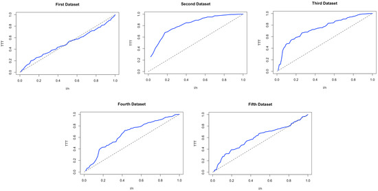
Figure 3. TTT plots for datasets.

• The Generalized Inverse Generalized Weibull Distribution (GIGW) given in (3).
• The Exponential Fréchet (NEXF) Distribution [5]
  $\hspace{1em}F\left(x\right)=1-{\displaystyle \frac{1-e^{-{(\lambda /x)}^{\beta }}}{e^{\theta e^{-{(\lambda /x)}^{\beta }}}}}$.
• The Exponentiated Generalized Inverse Weibull (EGIW) Distribution [31]
  $\hspace{1em}F\left(x\right)={[1-{\{1-e^{-{(\lambda /x)}^{\beta }}\}}^{\alpha }]}^q$.
• The Exponentiated Weibull Exponential (EWE) Distribution [36]
  $\hspace{1em}F\left(x\right)={[1-e^{-{\left(\frac{jx}{h}\right)}^k}]}^z$.
• The Inverse Weibull (IW) Distribution [37]
  $F\left(x\right)=e^{-{(\lambda /x)}^{\beta }}$.

As noted in Section 5, the ML demonstrated better results. MLs of the parameters for each distribution were computed along with their corresponding log-likelihood values. In order to assess the effectiveness of the NEGIGW, various goodness of fit (GoF) criteria were employed, namely the corrected Akaike information criterion (CAIC), Akaike information criterion (AIC), Bayesian information criterion (BIC), Hannan–Quinn information criterion (HQIC), and the Kolomogorov–Smirnov (K-S) test. The p-value corresponding to the K-S test is calculated. The optimal model is characterized by the minimum value of these statistics and the maximum p-value.

Table 5, Table 6, Table 7, Table 8 and Table 9 summarize the MLs of the parameters, the log-likelihood, and the GoF for each model. The results in Table 5, Table 6, Table 7, Table 8 and Table 9 indicate that the NEGIGW has the lowest CAIC, AIC, BIC, HQIC, and K-S measures. The NEGIGW has the highest p-values among all the fitted models. Furthermore, Figure 4, Figure 5, Figure 6, Figure 7 and Figure 8 display the density and CDF for the NEGIGW and the competitive distributions. The histogram represents the empirical density for the data and the dot black line represents the empirical CDF for the data. The Figures demonstrate that NEGIGW best matches the actual distribution of the examined datasets. Consequently, when compared to competing distributions, the NEGIGW is the most appropriate model for the analyzed data.

Table 5. Measures of ML and GoF for the first data.

Distributions	NEGIGW	GIGW	NEXF	EGIW	EWE	IW
Estimates	$\widehat{\theta }=$ 40.0485		$\widehat{\theta }=$ 11.1467	$\widehat{q}=$ 10.9153	$\widehat{j}=$ 0.4596
	$\widehat{\gamma }=$ 8.9609	$\widehat{\gamma }=$ 6.4492			$\widehat{k}=$ 0.5434
	$\widehat{\lambda }=$ 1.9341	$\widehat{\lambda }=$ 0.7863	$\widehat{\lambda }=$ 86.1435	$\widehat{\lambda }=$ 50.5093	$\widehat{h}=$ 0.7251	$\widehat{\lambda }=$ 3.2582
	$\widehat{\alpha }=$ 31.0659	$\widehat{\alpha }=$ 22.4685		$\widehat{\alpha }=$ 11.6619	$\widehat{z}=$ 5.8631
	$\widehat{\beta }=$ 0.1495	$\widehat{\beta }=$ 0.3052	$\widehat{\beta }=$ 0.3818	$\widehat{\beta }=$ 0.1951		$\widehat{\beta }=$ 0.7520
$-\ell$	−410.9638	−413.7740	−417.8249	−424.7263	−413.7165	−444.0008
CAIC	832.4194	835.8732	841.8433	857.7778	835.7582	892.0975
AIC	831.9276	835.5480	841.6498	857.4526	835.4330	892.0015
BIC	846.1877	846.9561	850.2059	868.8607	846.8412	897.7056
HQIC	837.7216	840.1832	845.1262	862.0878	840.0682	894.3191
K-S	0.0495	0.0578	0.0784	0.0934	0.0544	0.1407
p-value	0.9118	0.7848	0.4101	0.2138	0.8419	0.01250

Table 6. Measures of ML and GoF for the second data.

Distributions	NEGIGW	GIGW	NEXF	EGIW	EWE	IW
Estimates	$\widehat{\theta }=$ 113.6416		$\widehat{\theta }=$ 46.7096	$\widehat{q}=$ 88.8453	$\widehat{j}=$ 3.8269
	$\widehat{\gamma }=$ 10.7248	$\widehat{\gamma }=$ 49.1384			$\widehat{k}=$ 1.0587
	$\widehat{\lambda }=$ 4.6217	$\widehat{\lambda }=$ 0.1821	$\widehat{\lambda }=$ 41.7403	$\widehat{\lambda }=$ 12.8390	$\widehat{h}=$ 7.6894	$\widehat{\lambda }=$ 4.6721
	$\widehat{\alpha }=$ 97.6858	$\widehat{\alpha }=$ 71.4909		$\widehat{\alpha }=$ 14.9492	$\widehat{z}=$ 17.8675
	$\widehat{\beta }=$ 0.3634	$\widehat{\beta }=$ 0.6764	$\widehat{\beta }=$ 0.7394	$\widehat{\beta }=$ 0.3051		$\widehat{\beta }=$ 1.9445
$-\ell$	−84.98336	−87.92892	−88.71552	−97.82884	−93.78136	−101.5917
CAIC	181.7314	185.0007	184.0977	204.8005	196.7056	207.5079
AIC	179.9667	183.8578	183.4310	203.6577	195.5627	207.1836
BIC	188.4111	190.6134	188.4977	210.4132	202.3182	210.5613
HQIC	183.0199	186.3004	185.2630	206.1003	198.0053	208.4049
K-S	0.1175	0.1321	0.1372	0.2079	0.1261	0.2438
p-value	0.6379	0.4873	0.4381	0.0628	0.5481	0.0172

Table 7. Measures of ML and GoF for the third data.

Distributions	NEGIGW	GIGW	NEXF	EGIW	EWE	IW
Estimates	$\widehat{\theta }=$ 62.9467		$\widehat{\theta }=$ 38.6179	$\widehat{q}=$ 48.1213	$\widehat{j}=$ 7.0647
	$\widehat{\gamma }=$ 7.4028	$\widehat{\gamma }=$ 4.3172			$\widehat{k}=$ 0.3127
	$\widehat{\lambda }=$ 4.1741	$\widehat{\lambda }=$ 2.8629	$\widehat{\lambda }=$ 46.6470	$\widehat{\lambda }=$ 27.6062	$\widehat{h}=$ 0.1155	$\widehat{\lambda }=$ 1.4486
	$\widehat{\alpha }=$ 56.5685	$\widehat{\alpha }=$ 80.5273		$\widehat{\alpha }=$ 17.0032	$\widehat{z}=$ 69.9833
	$\widehat{\beta }=$ 0.2438	$\widehat{\beta }=$ 0.3792	$\widehat{\beta }=$ 0.4541	$\widehat{\beta }=$ 0.1619		$\widehat{\beta }=$ 0.8387
$-\ell$	−138.2479	−146.3092	−150.8618	−175.9310	−163.8430	−194.5367
CAIC	287.2651	301.1247	308.0236	360.3683	336.1922	393.2215
AIC	286.4959	300.6184	307.7236	359.8620	335.6859	393.0733
BIC	298.6500	310.3417	315.0160	369.5853	345.4092	397.9350
HQIC	291.3817	304.5271	310.6551	363.7707	339.5946	395.0277
K-S	0.1067	0.1455	0.1616	0.2334	0.1812	0.3127
p-value	0.2937	0.0569	0.0248	0.0002	0.0079	1.4533 $\times {10}^{-7}$

Table 8. Measures of ML and GoF for the fourth data.

Distributions	NEGIGW	GIGW	NEXF	EGIW	EWE	IW
Estimates	$\widehat{\theta }=$ 114.3494		$\widehat{\theta }=$ 60.2657	$\widehat{q}=$ 43.8506	$\widehat{j}=$ 7.0741
	$\widehat{\gamma }=$ 8.3534	$\widehat{\gamma }=$ 3.911			$\widehat{k}=$ 0.2408
	$\widehat{\lambda }=$ 4.4939	$\widehat{\lambda }=$ 3.1471	$\widehat{\lambda }=$ 68.1877	$\widehat{\lambda }=$ 48.6810	$\widehat{h}=$ 0.0186	$\widehat{\lambda }=$ 0.9307
	$\widehat{\alpha }=$ 97.7212	$\widehat{\alpha }=$ 77.6282		$\widehat{\alpha }=$ 28.6196	$\widehat{z}=$ 69.9850
	$\widehat{\beta }=$ 0.1560	$\widehat{\beta }=$ 0.2879	$\widehat{\beta }=$ 0.3961	$\widehat{\beta }=$ 0.1765		$\widehat{\beta }=$ 0.8102
$-\ell$	−103.7424	−108.1407	−115.3408	−144.9830	−117.5368	−131.3029
CAIC	218.5375	224.9711	237.0883	298.6557	243.7633	266.8058
AIC	217.4849	224.2814	236.6816	297.9660	243.0736	266.6058
BIC	228.2005	232.8539	243.1110	306.5385	251.6461	270.8921
HQIC	221.6994	227.6530	239.2103	301.3376	246.4452	268.2916
K-S	0.1406	0.1626	0.2184	0.3978	0.1752	0.2215
p-value	0.1499	0.0635	0.0041	1.65 $\times {10}^{-9}$	0.0366	1.49 $\times {10}^{-1}$

Table 9. Measures of ML and GoF for the fifth data.

Distributions	NEGIGW	GIGW	NEXF	EGIW	EWE	IW
Estimates	$\widehat{\theta }=$ 36.4168		$\widehat{\theta }=$ 13.5573	$\widehat{q}=$ 0.5567	$\widehat{j}=$ 3.9945
	$\widehat{\gamma }=$ 1.0614	$\widehat{\gamma }=$ 3.911			$\widehat{k}=$ 0.5579
	$\widehat{\lambda }=$ 3.4524	$\widehat{\lambda }=$ 1.0997	$\widehat{\lambda }=$ 21.1117	$\widehat{\lambda }=$ 50.4851	$\widehat{h}=$ 1.3137	$\widehat{\lambda }=$ 0.8207
	$\widehat{\alpha }=$ 31.4465	$\widehat{\alpha }=$ 0.6286		$\widehat{\alpha }=$ 28.4964	$\widehat{z}=$ 7.0722
	$\widehat{\beta }=$ 0.1811	$\widehat{\beta }=$ 0.8498	$\widehat{\beta }=$ 0.4038	$\widehat{\beta }=$ 0.4141		$\widehat{\beta }=$ 0.7588
$-\ell$	−123.6436	−127.4275	−131.5939	−127.7306	−126.4810	−153.5392
CAIC	258.1444	263.4185	269.5211	264.0246	261.5253	311.2428
AIC	257.2873	262.8551	269.1877	263.4612	260.9619	311.0784
BIC	268.9409	272.1780	276.1799	272.7841	270.2848	315.7399
HQIC	261.9446	266.5810	271.9821	267.1871	264.6878	312.9414
K-S	0.0845	0.1044	0.1310	0.1177	0.0934	0.1893
p-value	0.6179	0.3540	0.1343	0.2239	0.4918	7.37 $\times {10}^{-3}$

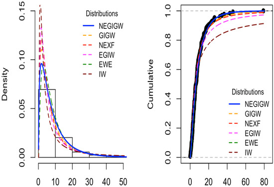
Figure 4. The NEGIGW is compared to other distributions for the first data. (Right): CDF for all distributions. (Left): observed and expected frequencies for all distributions.

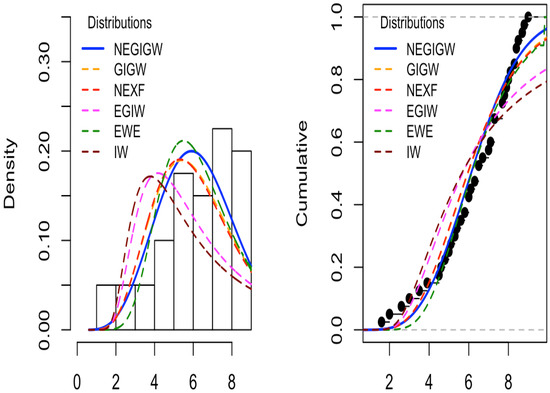
Figure 5. The NEGIGW is compared to other distributions for the second data. (Right): CDF for all distributions. (Left): observed and expected frequencies for all distributions.

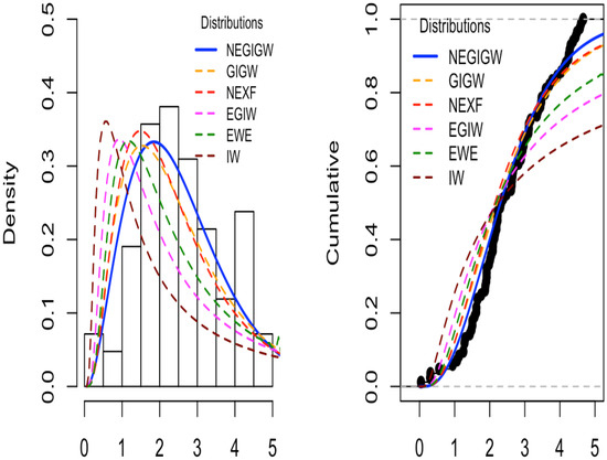
Figure 6. The NEGIGW is compared to other distributions for the third data. (Right): CDF for all distributions. (Left): observed and expected frequencies for all distributions.

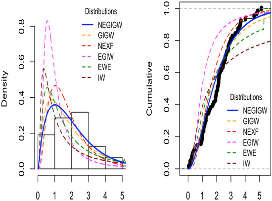
Figure 7. The NEGIGW is compared to other distributions for the fourth data. (Right): CDF for all distributions. (Left): observed and expected frequencies for all distributions.

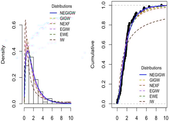
Figure 8. The NEGIGW is compared to other distributions for the fifth data. (Right): CDF for all distributions. (Left): observed and expected frequencies for all distributions.

7. Concluding Remarks

This article introduces a new exponential generalized inverse generalized Weibull (NEGIGW) distribution based on the NLTE-X family. The suggested NEGIGW was motivated by the idea that generalization gives more flexibility in examining practical data. The NEGIGW’s hazard rate function takes several forms, allowing it to mimic various hazard behaviors in real-world settings such as medical, biological, engineering, and other applications. Important statistical properties are derived in close form. The estimation of the NEGIGW’s parameters is obtained using three methods of estimation; ML, MPS, and PC. An extensive simulation study is performed to compare the performance of these methods. The simulation results indicate that in terms of MSEs, the ML performs better than other methods. Five applications from medical, biological, and engineering fields are used to demonstrate the usefulness of the NEGIGW. We concluded that the proposed NEGIGW fits better than other competing models. This generalization is expected to lead to further lifetimes and reliability analysis applications.

References

- Eugene, N.; Lee, C.; Famoye, F. Beta-normal distribution and its applications. Commun. Stat.-Theory Methods 2002, 31, 497–512. [Google Scholar] [CrossRef]
- Jones, M. Kumaraswamy’s distribution: A beta-type distribution with some tractability advantages. Stat. Methodol. 2009, 6, 70–81. [Google Scholar] [CrossRef]
- Alzaatreh, A.; Lee, C.; Famoye, F. A new method for generating families of continuous distributions. Metron 2013, 71, 63–79. [Google Scholar] [CrossRef]
- Huo, X.; Khosa, S.K.; Ahmad, Z.; Almaspoor, Z.; Ilyas, M.; Aamir, M. A new lifetime exponential-X family of distributions with applications to reliability data. Math. Probl. Eng. 2020, 2020, 1316345. [Google Scholar] [CrossRef]
- Alzeley, O.; Almetwally, E.M.; Gemeay, A.M.; Alshanbari, H.M.; Hafez, E.H.; Abu-Moussa, M. Statistical inference under censored data for the new exponential-X Fréchet distribution: Simulation and application to leukemia data. Comput. Intell. Neurosci. 2021, 2021, 2167670. [Google Scholar] [CrossRef] [PubMed]
- Metwally, A.S.M.; Hassan, A.S.; Almetwally, E.M.; Kibria, B.G.; Almongy, H.M. Reliability analysis of the new exponential inverted Topp–Leone distribution with applications. Entropy 2021, 23, 1662. [Google Scholar] [CrossRef] [PubMed]
- Hassan, F.; Hafez, E.A. The exponential-X power function (NEXPF) distribution and its applications to modelling reliability. J. Algebr. Stat. 2022, 13, 741–752. [Google Scholar]
- Khan, M.S.; Pasha, G.; Pasha, A.H. Theoretical analysis of inverse Weibull distribution. WSEAS Trans. Math. 2008, 7, 30–38. [Google Scholar]
- Mudholkar, G.S.; Srivastava, D.K.; Kollia, G.D. A generalization of the Weibull distribution with application to the analysis of survival data. J. Am. Stat. Assoc. 1996, 91, 1575–1583. [Google Scholar] [CrossRef]
- Abd AL-Fattah, A.; El-Helbawy, A.; Al-Dayian, G. Inverted Kumaraswamy distribution: Properties and estimation. Pak. J. Stat. 2017, 33, 37–61. [Google Scholar]
- Hassan, A.S.; Elgarhy, M.; Ragab, R. Statistical properties and estimation of inverted Topp-Leone distribution. J. Stat. Appl. Probab. 2020, 9, 319–331. [Google Scholar]
- Shahbaz, M.Q.; Shahbaz, S.; Butt, N.S. The Kumaraswamy-inverse Weibull distribution. Pak. J. Stat. Oper. Res. 2012, 8, 479–489. [Google Scholar] [CrossRef]
- Oguntunde, P.; Adejumo, A.O.; Owoloko, E. Application of Kumaraswamy inverse exponential distribution to real lifetime data. Int. J. Appl. Math. Stat. 2017, 56, 34–47. [Google Scholar]
- Malik, A.; Ahmad, S. A new inverse Rayleigh distribution: Properties and application. Int. J. Sci. Res. Math. Stat. Sci. 2018, 5, 92–96. [Google Scholar] [CrossRef]
- Rao, G.S.; Mbwambo, S. Exponentiated inverse Rayleigh distribution and an application to coating weights of iron sheets data. J. Probab. Stat. 2019, 2019, 7519429. [Google Scholar] [CrossRef]
- Eghwerido, J. A new Weibull inverted exponential distribution: Properties and applications. FUPRE J. Sci. Ind. Res. (FJSIR) 2022, 6, 58–72. [Google Scholar]
- Basheer, A.M.; Almetwally, E.M.; Okasha, H.M. Marshall-Olkin alpha power inverse Weibull distribution: Non bayesian and bayesian estimations. J. Stat. Appl. Probab. 2021, 10, 327–345. [Google Scholar]
- Ali, M.; Khalil, A.; Ijaz, M.; Saeed, N. Alpha-power exponentiated inverse Rayleigh distribution and its applications to real and simulated data. PLoS ONE 2021, 16, e0245253. [Google Scholar] [CrossRef] [PubMed]
- Almetwally, E.M. The odd Weibull inverse Topp–leone distribution with applications to COVID-19 data. Ann. Data Sci. 2022, 9, 121–140. [Google Scholar] [CrossRef] [PubMed]
- Hassan, A.S.; Elsherpieny, E.A.; Mohamed, R.E. Odds generalized exponential-inverse Weibull distribution: Properties & estimation. Pak. J. Stat. Oper. Res. 2018, 14, 1–22. [Google Scholar]
- Iqbal, Z.; Tahir, M.M.; Riaz, N.; Ali, S.A.; Ahmad, M. Generalized inverted Kumaraswamy distribution: Properties and application. Open J. Stat. 2017, 7, 645. [Google Scholar] [CrossRef]
- Ogunde, A.A.; Chukwu, A.U.; Oseghale, I.O. The Kumaraswamy Generalized Inverse Lomax distribution and applications to reliability and survival data. Sci. Afr. 2023, 19, e01483. [Google Scholar] [CrossRef]
- Hassan, A.S.; Nassr, S.G. The Inverse Weibull generator of distributions: Properties and applications. J. Data Sci. 2018, 16, 723–742. [Google Scholar] [CrossRef]
- De Gusmao, F.R.; Ortega, E.M.; Cordeiro, G.M. The generalized inverse Weibull distribution. Stat. Pap. 2011, 52, 591–619. [Google Scholar] [CrossRef]
- Jain, K.; Singla, N.; Sharma, S.K. The generalized inverse generalized Weibull distribution and its properties. J. Probab. 2014, 2014, 736101. [Google Scholar] [CrossRef]
- Rao, A.K.; Pandey, H. Parameter estimation of generalized inverse generalized Weibull distribution via Bayesian approach. Eur. Sch. J. 2022, 3, 23–28. [Google Scholar]
- Rényi, A. On measures of information and entropy. In Proceedings of the 4th Berkeley Symposium on Mathematics, Statistics and Probability, Berkeley, CA, USA, 20–30 June 1961; Volume 1. [Google Scholar]
- Cheng, R.; Amin, N. Maximum product-of-spacings estimation with applications to the lognormal distribution. Math Rep. 1979, 791. [Google Scholar]
- Schoonjans, F.; De Bacquer, D.; Schmid, P. Estimation of population percentiles. Epidemiology 2011, 22, 750–751. [Google Scholar] [CrossRef]
- R Core Team. R: A Language and Environment for Statistical Computing; R Foundation for Statistical Computing: Vienna, Austria, 2024. [Google Scholar]
- Elbatal, I.; Muhammed, H.Z. Exponentiated generalized inverse Weibull distribution. Appl. Math. Sci. 2014, 8, 3997–4012. [Google Scholar] [CrossRef]
- Xu, K.; Xie, M.; Tang, L.C.; Ho, S.L. Application of neural networks in forecasting engine systems reliability. Appl. Soft Comput. 2003, 2, 255–268. [Google Scholar] [CrossRef]
- Tahir, M.H.; Cordeiro, G.M.; Mansoor, M.; Zubair, M. The Weibull-Lomax distribution: Properties and applications. Hacet. J. Math. Stat. 2015, 44, 455–474. [Google Scholar] [CrossRef]
- Abdul-Moniem, I.; Seham, M. Transmuted gompertz distribution. Comput. Appl. Math. J. 2015, 1, 88–96. [Google Scholar]
- Aarset, M.V. How to identify a bathtub hazard rate. IEEE Trans. Reliab. 1987, 36, 106–108. [Google Scholar] [CrossRef]
- Alsolami, E.; Alsulami, D. Combining two exponentiated families to generate a new family of distributions. Symmetry 2022, 14, 1739. [Google Scholar] [CrossRef]
- Keller, A.Z.; Kamath, A.R.R. Alternative reliability models for mechanical systems. In Proceedings of the Third International Conference on Reliability and Maintainability, Toulouse, France, 18–22 October 1982; pp. 411–415. [Google Scholar]
Disclaimer/Publisher’s Note: The statements, opinions and data contained in all publications are solely those of the individual author(s) and contributor(s) and not of MDPI and/or the editor(s). MDPI and/or the editor(s) disclaim responsibility for any injury to people or property resulting from any ideas, methods, instructions or products referred to in the content. |
© 2024 by the authors. Licensee MDPI, Basel, Switzerland. This article is an open access article distributed under the terms and conditions of the Creative Commons Attribution (CC BY) license (https://creativecommons.org/licenses/by/4.0/).