New Numerical Results on Existence of Volterra–Fredholm Integral Equation of Nonlinear Boundary Integro-Differential Type

Abstract

Symmetry is presented in many works involving differential and integral equations. Whenever a human is involved in the design of an integral equation, they naturally tend to opt for symmetric features. The most common examples are the Green functions and linguistic kernels that are often designed symmetrically and regularly distributed over the universe of discourse. In the current study, the authors report a study on boundary value problem (BVP) for a nonlinear integro Volterra–Fredholm integral equation with variable coefficients and show the existence of solution by applying some fixed-point theorems. The authors employ various numerical common approaches as the homotopy analysis methodology established by Liao and the modified Adomain decomposition technique to produce a numerical approximate solution, then graphical depiction reveals that both methods are most effective and convenient. In this regard, the authors address the requirements that ensure the existence and uniqueness of the solution for various variations of nonlinearity power. The authors also show numerical examples of how to apply our primary theorems and test the convergence and validity of our suggested approach.

1. Basic Tools and Existence of Solutions

In this section we briefly review some basic elements of the Volterra–Fredholm integral equations and integro-differential equations. For a comprehensive study on these topics, we refer the interested reader to [33,34,35,36,37].

Definition 1

(See [33]). Let $(X,\mathrm{d})$ be a metric space. Then, we say a function $\mathtt{f}$:$X\to X$ is a contraction mapping, if there is a non-negative real number $0\le k<1$ such that

$$\begin{array}{c}\hfill \mathrm{d}\left(\mathtt{f}\right(\mathtt{x}),\mathtt{f}(\mathtt{y}\left)\right)\le k\mathrm{d}(\mathtt{x},\mathtt{y}),for all\mathtt{x},\mathtt{y}\in X.\end{array}$$

Theorem 1

(See [37]). Suppose that $g\left(\mathtt{x}\right)=li{m}_{n\to \infty }{g}_n\left(\mathtt{x}\right)$ on J, where $g,g_1,g_2,\dots$ are all Riemann integrable functions on I. If ${\left\{g_n\left(x\right)\right\}}_{n=1}^{\infty }$ is uniformly bounded on J, then ${\int }_{b_0}^{b_1}g\left(\mathtt{t}\right)\mathrm{d}\mathtt{t}=li{m}_{n\to \infty }{\int }_{b_0}^{b_1}{g}_n\left(\mathtt{t}\right)\mathrm{d}\mathtt{t}$ and $li{m}_{n\to \infty }{\int }_{b_0}^{b_1}\left|g_n\left(\mathtt{t}\right)-g\left(\mathtt{t}\right)\right|\mathrm{d}\mathtt{t}=0$

Theorem 2

(See [34]). Let $(X,\mathrm{d})$ be a metric space, then for each contraction mapping ${\tau }:X\to X$ has a unique fixed point of τ in X.

Theorem 3

(See [35]). Let $(X,||.|\left|\right)$ be a Banach space over $\mathbb{R}$ and $\mathcal{K}$ be a nonempty closed, convex and bounded subset of X. Any Compact operator $b_0:\mathcal{K}\to \mathcal{K}$ has at least one fixed point.

Our two theorems are considering the Arzela–Ascoli theorem and Krasnoselskii fixed point theorem, respectively.

Theorem 4

(See [33]). Every bounded and equicontinuous sequence in the closed and bounded interval $[a,b]$ has a uniformly convergent subsequence.

Theorem 5

(See [36]). Let X be a Banach space and μ be a closed and convex nonempty subset of X, then the functions $\mathcal{H},\mathcal{K}:\mu \to X$ with the following properties:

1. 

$\mathcal{H}$ is a contraction mapping,

2. 

$\mathcal{K}$ is compact and continuous,

3. 

for all $\mathtt{x},\mathtt{y}\in \mu$, such that $\mathcal{H}\mathtt{x}+\mathcal{K}\mathtt{y}\in \mu .$

Then, there is $\mathtt{y}$ in μ such that $\mathcal{H}\mathtt{y}+\mathcal{K}\mathtt{y}=\mathtt{y}$.

Let us briefly recall the following concepts that will be involved in proving the next theorem of existence and uniqueness of the solutions.

Main postulates:

We suppose the following Hypotheses to prove all theorems.

Hypothesis 1

(H1). The functions $\mathcal{A}$ and $\mathcal{B}$ belong to $\mathcal{C}(J,\mathbb{R})$.

Hypothesis 2

(H2). The known free function $\mathtt{f}$ is a member of the ${\mathcal{C}}^2(J,\mathbb{R})$.

Hypothesis 3

(H3). For any $\mathtt{y}\in J$, the known kernel $(\mathtt{t},\mathtt{y})\mapsto {\Psi }(\mathtt{t},\mathtt{y})$ is continuous in $\mathtt{t}$, for all $\mathtt{t}\in \mathbb{R}$.

$${\left(\underset{b_0}{\overset{b_1}{\int }}{\left({\Psi }(\mathtt{t},\mathtt{y})\right)}^{2}dy\right)}^{\frac{1}{2}}\le \gamma ,\mathrm{for} \mathrm{all}\mathtt{t}\in J,\gamma >0,$$

Hypothesis 4

(H4).

$$\left(\xi +k_1|{{\lambda }}_1|{{\epsilon }}_1\left(1\right)+\left|{{\lambda }}_2\right|{{\epsilon }}_2\left(1\right)\right)\le |\mho |,$$

where

$$\xi =\left((b_1-b_0){\parallel \mathcal{A}\parallel }_{\infty }+{(b_1-b_0)}^2{\parallel \mathcal{B}\parallel }_{\infty }\right),$$

$${{\epsilon }}_1\left(l\right)=\left(\genfrac{}{}{0pt}{}{p}{l}\right)\frac{\gamma {(b_1-b_0)}^{2l+\frac{1}{2}}\sqrt{{{{\rm Y}}}_1\left(l\right)}}{\sqrt{2p-2l+1}},$$

$${{\epsilon }}_2\left(l\right)=\left(\genfrac{}{}{0pt}{}{q}{l}\right)\frac{\gamma {(b_1-b_0)}^{2l+\frac{1}{2}}\sqrt{{{{\rm Y}}}_2\left(l\right)}}{\sqrt{2q-2l+1}},$$

$${{{\rm Y}}}_1\left(l\right)=\left\{{\ell }_2^{2p-2l}+{\ell }_2^{2p-2l-1}{\ell }_1+\cdots +{\ell }_1^{2p-2l}\right\},$$

and

$${{{\rm Y}}}_2\left(l\right)=\left\{{\ell }_2^{2q-2l}+{\ell }_2^{2q-2l-1}{\ell }_1+\cdots +{\ell }_1^{2q-2l}\right\}.$$

Hypothesis 5

(H5).

$$\left(\xi +|{{\lambda }}_1|{{\Lambda }}_1+\left|{{\lambda }}_2\right|{{\Lambda }}_2\right)\le |\mho |,$$

where

$${{\Lambda }}_1=\sum _{l=1}^p{\displaystyle \frac{{\rho }_1\left(l\right)k_1^l{{\epsilon }}_1\left(l\right)}{{(b_1-b_0)}^{3l-3}}},$$

and

$${{\Lambda }}_2=\sum _{l=1}^q{\displaystyle \frac{{\rho }_2\left(l\right){{\epsilon }}_2\left(l\right)}{{(b_1-b_0)}^{3l-3}}},$$

where ${\rho }_1\left(l\right),{\rho }_2\left(l\right)\mathrm{such} \mathrm{that}{\rho }_1\left(1\right)=1={\rho }_2\left(1\right)$ are finite positive constants depend on l and $k_1$ is a positive real numbers.

Theorem 6.

If the conditions $\left(\mathbf{H}\mathbf{1}\right)$–$\left(\mathbf{H}\mathbf{3}\right)$ are applied, then (1)–(2) are reduce to the as follows Equation (3) is nonlinear Volterra–Fredholm integral equations (NVFIE).

$$\begin{array}{cc}\hfill \mho \sigma \left(\mathtt{t}\right)& +\underset{b_0}{\overset{b_1}{\int }}[\mathcal{H}(\mathtt{t},\mathtt{x})-{{\lambda }}_1\underset{b_0}{\overset{\mathtt{t}}{\int }}{\mathcal{S}}_p(\mathtt{t},\mathtt{y};1){\mathcal{M}}_2(\mathtt{y},\mathtt{x})\mathrm{d}\mathtt{y}\hfill \\ \hfill & -{{\lambda }}_2\underset{b_0}{\overset{b_1}{\int }}{\mathcal{S}}_q(\mathtt{t},\mathtt{y};1){\mathcal{M}}_2(\mathtt{y},\mathtt{x})\mathrm{d}\mathtt{y}]\sigma \left(\mathtt{x}\right)\mathrm{d}\mathtt{x}\hfill \\ \hfill & =\mathcal{F}\left(\mathtt{t}\right)+{{\lambda }}_1\underset{b_0}{\overset{\mathtt{t}}{\int }}\sum _{l=2}^p{\mathcal{S}}_p(\mathtt{t},\mathtt{y};l){\left(\underset{b_0}{\overset{b_1}{\int }}{\mathcal{M}}_2(\mathtt{y},\mathtt{x})\sigma \left(\mathtt{x}\right)\mathrm{d}\mathtt{x}\right)}^l\mathrm{d}\mathtt{y}\hfill \\ \hfill & +{{\lambda }}_2\underset{b_0}{\overset{b_1}{\int }}\sum _{l=2}^q{\mathcal{S}}_q(\mathtt{t},\mathtt{y};l){\left(\underset{b_0}{\overset{b_1}{\int }}{\mathcal{M}}_2(\mathtt{y},\mathtt{x})\sigma \left(\mathtt{x}\right)\mathrm{d}\mathtt{x}\right)}^l\mathrm{d}\mathtt{y},\hfill \end{array}$$

(3)

where

$$\begin{array}{ccc}\hfill \sigma \left(\mathtt{t}\right)& :=& {{\phi }}^{{}^{″}}\left(\mathtt{t}\right),\hfill \end{array}$$

(4)

$$\begin{array}{ccc}\hfill \mathcal{H}(\mathtt{t},\mathtt{x})& :=& {\displaystyle \frac{1}{(b_1-b_0)}}\left\{\begin{array}{cc}(\mathtt{x}-b_0)\left(\mathcal{A}\left(\mathtt{t}\right)-(b_1-\mathtt{t})\mathcal{B}\left(\mathtt{t}\right)\right)\hfill & b_0\le \mathtt{x}\le \mathtt{t}\hfill \\ (\mathtt{x}-b_1)\left(\mathcal{A}\left(\mathtt{t}\right)-(b_0-\mathtt{t})\mathcal{B}\left(\mathtt{t}\right)\right)\hfill & \mathtt{t}\le \mathtt{x}\le b_1\hfill \end{array}\right.,\hfill \end{array}$$

(5)

$$\begin{array}{ccc}\hfill {\mathcal{S}}_p(\mathtt{t},\mathtt{y};l)& :=& \left(\genfrac{}{}{0pt}{}{p}{l}\right){\displaystyle \frac{{\Psi }(\mathtt{t},\mathtt{y})}{{(b_1-b_0)}^p}}{\left[{\ell }_1(b_1-\mathtt{y})+{\ell }_2(\mathtt{y}-b_0)\right]}^{p-l},\hfill \end{array}$$

(6)

$$\begin{array}{ccc}\hfill {\mathcal{S}}_q(\mathtt{t},\mathtt{y};l)& :=& \left(\genfrac{}{}{0pt}{}{q}{l}\right){\displaystyle \frac{{\Psi }(\mathtt{t},\mathtt{y})}{{(b_1-b_0)}^q}}{\left[{\ell }_1(b_1-\mathtt{y})+{\ell }_2(\mathtt{y}-b_0)\right]}^{q-l},\hfill \end{array}$$

(7)

$$\begin{array}{ccc}\hfill {\mathcal{M}}_2(\mathtt{y},\mathtt{x})& :=& \left\{\begin{array}{cc}(\mathtt{x}-b_0)(\mathtt{y}-b_1)\hfill & b_0\le \mathtt{x}\le \mathtt{y}\hfill \\ (\mathtt{x}-b_1)(\mathtt{y}-b_0)\hfill & \mathtt{y}\le \mathtt{x}\le b_1\hfill \end{array}\right.,\hfill \end{array}$$

(8)

$$\begin{array}{ccc}\hfill \mu \left(\mathtt{t}\right)& :=& {\displaystyle \frac{\left(-\mathcal{A}\left(\mathtt{t}\right)+(b_1-\mathtt{t})\mathcal{B}\left(\mathtt{t}\right)\right){\ell }_1+\left(\mathcal{A}\left(\mathtt{t}\right)+(\mathtt{t}-b_0)\mathcal{B}\left(\mathtt{t}\right)\right){\ell }_2}{(b_1-b_0)}},\hfill \end{array}$$

(9)

$$\begin{array}{ccc}\hfill \mathcal{F}\left(\mathtt{t}\right)& :=& \mathtt{f}\left(\mathtt{t}\right)+{{\lambda }}_1\underset{b_0}{\overset{\mathtt{t}}{\int }}{\mathcal{S}}_p(\mathtt{t},\mathtt{y};0)\mathrm{d}\mathtt{y}+{{\lambda }}_2\underset{b_0}{\overset{b_1}{\int }}{\mathcal{S}}_q(\mathtt{t},\mathtt{y};0)\mathrm{d}\mathtt{y}-\mu \left(\mathtt{t}\right).\hfill \end{array}$$

(10)

Proof. 

If a function $\mathtt{t}\mapsto \sigma \left(\mathtt{t}\right)$ belongs $C(J,\mathbb{R})$, then:

$$Let{{\phi }}^{{}^{″}}\left(\mathtt{t}\right)=\sigma \left(\mathtt{t}\right),$$

(11)

$${{\phi }}^{{}^{\prime }}\left(\mathtt{t}\right)=\underset{b_0}{\overset{\mathtt{t}}{\int }}\sigma \left(\mathtt{x}\right)\mathrm{d}\mathtt{x}+{{\phi }}^{{}^{\prime }}\left(b_0\right),$$

(12)

and

$${\phi }\left(\mathtt{t}\right)=\underset{b_0}{\overset{\mathtt{t}}{\int }}(\mathtt{t}-\mathtt{x})\sigma \left(\mathtt{x}\right)\mathrm{d}\mathtt{x}+{\ell }_1+(\mathtt{t}-b_0){{\phi }}^{{}^{\prime }}\left(b_0\right).$$

(13)

It follows from Equation (13) with $\mathtt{t}=b_1$ that

$${{\phi }}^{{}^{\prime }}\left(b_0\right)=\frac{1}{(b_1-b_0)}\left[({\ell }_2-{\ell }_1)+\underset{b_0}{\overset{b_1}{\int }}(x-b_0)\sigma \left(x\right)dx\right]$$

(14)

and by putting Equation (14) into Equation (12), we obtain

$${{\phi }}^{{}^{\prime }}\left(\mathtt{t}\right)={\displaystyle \frac{1}{(b_1-b_0)}}\left[({\ell }_2-{\ell }_1)+\underset{b_0}{\overset{b_1}{\int }}{\mathcal{H}}_1(\mathtt{t},\mathtt{x})\sigma \left(\mathtt{x}\right)\mathrm{d}\mathtt{x}\right].$$

(15)

By using the result in Equations (12) and (11), we can obtain

$${\phi }\left(\mathtt{t}\right)={\displaystyle \frac{1}{(b_1-b_0)}}\left[(\mathtt{t}-b_0){\ell }_2+(b_1-\mathtt{x}){\ell }_1+\underset{b_0}{\overset{b_1}{\int }}{\mathcal{H}}_2(\mathtt{t},\mathtt{x})\sigma \left(\mathtt{x}\right)\mathrm{d}\mathtt{x}\right],$$

(16)

where

$${\mathcal{M}}_1(\mathtt{t},\mathtt{x}):=\left\{\begin{array}{cc}(b_0-\mathtt{x})\hfill & b_0\le \mathtt{x}\le \mathtt{t}\hfill \\ (b_1-\mathtt{x})\hfill & \mathtt{t}\le \mathtt{x}\le b_1\hfill \end{array}\right.,$$

(17)

$${\mathcal{M}}_2(\mathtt{t},\mathtt{x}):=\left\{\begin{array}{cc}(b_1-\mathtt{t})(b_0-\mathtt{x})\hfill & b_0\le \mathtt{x}\le \mathtt{x}\hfill \\ (b_0-\mathtt{t})(b_1-\mathtt{x})\hfill & \mathtt{t}\le \mathtt{x}\le b_1\hfill \end{array}\right.,$$

(18)

and

$${\left[{\phi }\left(\mathtt{t}\right)\right]}^p={\displaystyle \frac{1}{{(b_1-b_0)}^p}}\sum _{l=0}^p\left(\genfrac{}{}{0pt}{}{p}{l}\right){\left[(\mathtt{t}-b_0){\ell }_2+(b_1-\mathtt{t}){\ell }_1\right]}^{p-l}{\left(\underset{b_0}{\overset{b_1}{\int }}{\mathcal{M}}_2(\mathtt{t},\mathtt{x})\sigma \left(\mathtt{x}\right)\mathrm{d}\mathtt{x}\right)}^l,$$

(19)

$${\left[{\phi }\left(\mathtt{t}\right)\right]}^q={\displaystyle \frac{1}{{(b_1-b_0)}^q}}\sum _{l=0}^q\left(\genfrac{}{}{0pt}{}{q}{l}\right){\left[{\ell }_1(b_1-\mathtt{t})+{\ell }_2(\mathtt{t}-b_0)\right]}^{q-l}{\left(\underset{b_0}{\overset{b_1}{\int }}{\mathcal{M}}_2(\mathtt{t},\mathtt{x})\sigma \left(\mathtt{x}\right)\mathrm{d}\mathtt{x}\right)}^l.$$

(20)

Substitution Equations (11), (15), (16), (19) and (20) into Equation (1) to get

$$\begin{array}{cc}\hfill & \mho \sigma \left(\mathtt{t}\right)+{\displaystyle \frac{\mathcal{A}\left(\mathtt{t}\right)}{b_1-b_0}}\left({\ell }_2-{\ell }_1\right)+\frac{1}{b_1-b_0}\underset{b_0}{\overset{b_1}{\int }}\left[\mathcal{A}\left(\mathtt{t}\right)M_1(t,x)+\mathcal{B}\left(\mathtt{t}\right){\mathcal{M}}_2(\mathtt{t},\mathtt{x})\right]\sigma \left(\mathtt{x}\right)\mathrm{d}\mathtt{x}\hfill \\ \hfill & +{\displaystyle \frac{\mathcal{B}\left(\mathtt{t}\right)}{b_1-b_0}}\left((b_1-\mathtt{t}){\ell }_1+(\mathtt{t}-b_0){\ell }_2\right)\hfill \\ \hfill & =\mathcal{F}\left(\mathtt{t}\right)+{\displaystyle \frac{{{\lambda }}_1}{{(b_1-b_0)}^p}}\underset{b_0}{\overset{\mathtt{t}}{\int }}\sum _{l=0}^p\left(\genfrac{}{}{0pt}{}{p}{l}\right){\Psi }(\mathtt{t},\mathtt{y}){\left[(b_1-\mathtt{t}){\ell }_1+(\mathtt{t}-b_0){\ell }_2\right]}^{p-l}{\left(\underset{b_0}{\overset{b_1}{\int }}{\mathcal{M}}_2(\mathtt{y},\mathtt{x})\sigma \left(\mathtt{x}\right)\mathrm{d}\mathtt{x}\right)}^l\mathrm{d}\mathtt{y}\hfill \\ \hfill & +{\displaystyle \frac{{{\lambda }}_2}{{(b_1-b_0)}^q}}\underset{b_0}{\overset{b_1}{\int }}\sum _{l=0}^q\left(\genfrac{}{}{0pt}{}{q}{l}\right){\Psi }(\mathtt{t},\mathtt{y}){\left[(b_1-\mathtt{t}){\ell }_1+(\mathtt{t}-b_0){\ell }_2\right]}^{q-l}{\left(\underset{b_0}{\overset{b_1}{\int }}{\mathcal{M}}_2(\mathtt{y},\mathtt{x})\sigma \left(\mathtt{x}\right)\mathrm{d}\mathtt{x}\right)}^l\mathrm{d}\mathtt{y},\hfill \end{array}$$

$$\begin{array}{cc}\hfill \mho \sigma \left(\mathtt{t}\right)+\underset{b_0}{\overset{b_1}{\int }}[\mathcal{H}(\mathtt{t},\mathtt{x})& -{{\lambda }}_1\underset{b_0}{\overset{\mathtt{t}}{\int }}{\mathcal{S}}_p(\mathtt{t},\mathtt{y};1){\mathcal{M}}_2(\mathtt{y},\mathtt{x})\mathrm{d}\mathtt{y}-{{\lambda }}_2\underset{b_0}{\overset{b_1}{\int }}{\mathcal{S}}_q(\mathtt{t},\mathtt{y};1){\mathcal{M}}_2(\mathtt{y},\mathtt{x})\mathrm{d}\mathtt{y}]\sigma \left(\mathtt{x}\right)\mathrm{d}\mathtt{x}\hfill \\ \hfill & =\mathcal{F}\left(\mathtt{t}\right)+{{\lambda }}_1\underset{b_0}{\overset{\mathtt{t}}{\int }}\sum _{l=2}^p{\mathcal{S}}_p(\mathtt{t},\mathtt{y};l){\left(\underset{b_0}{\overset{b_1}{\int }}{\mathcal{M}}_2(\mathtt{y},\mathtt{x})\sigma \left(\mathtt{x}\right)\mathrm{d}\mathtt{x}\right)}^l\mathrm{d}\mathtt{y}\hfill \\ \hfill & +{{\lambda }}_2\underset{b_0}{\overset{b_1}{\int }}\sum _{l=2}^q{\mathcal{S}}_q(\mathtt{t},\mathtt{y};l){\left(\underset{b_0}{\overset{b_1}{\int }}{\mathcal{M}}_2(\mathtt{y},\mathtt{x})\sigma \left(\mathtt{x}\right)\mathrm{d}\mathtt{x}\right)}^l\mathrm{d}\mathtt{y},\hfill \end{array}$$

(21)

where $\mathcal{F}\left(\mathtt{t}\right),\mathcal{H}(\mathtt{t},\mathtt{x}),{\mathcal{S}}_p(\mathtt{t},\mathtt{y};l),{\mathcal{S}}_q(\mathtt{t},\mathtt{y};l)$ and $\mu \left(\mathtt{t}\right)$ are determined in Equations (5)–(7), (9) and (10) above, respectively.

The converse is straight forward and thereby it is omitted. □

The following theorem states that if the NVFIE (3) has a continuous solution if it meet the requirements $\left(\mathbf{H}\mathbf{1}\right)$–$\left(\mathbf{H}\mathbf{4}\right)$.

Theorem 7.

If conditions $\left(\mathbf{H}\mathbf{1}\right)$–$\left(\mathbf{H}\mathbf{4}\right)$ hold, then an NVFIE (3) has a continuous solution.

Proof. 

Let ${\nabla }_{\varsigma }=\{{\parallel \sigma \parallel }_{\infty }=\underset{\mathtt{t}\in J}{sup}\left|\sigma \left(\mathtt{t}\right)\right|\le \varsigma ,\sigma \in \mathcal{C}(J,\mathbb{R})\}$. Where the positive, finite solution of the Equation (22) is denoted by the symbol $\varsigma$.

$$|{{\lambda }}_1|\sum _{l=1}^p{\left(k_1\varsigma \right)}^l{{\epsilon }}_1\left(l\right)+|{{\lambda }}_2|\sum _{l=1}^q{\varsigma }^l{{\epsilon }}_2\left(l\right)+\left(\xi -|\mho |\right)\varsigma +{\parallel \mathcal{F}\parallel }_{\infty }=0,$$

(22)

and $k_1$ is an upper bound of $|{\mathcal{M}}_2(\mathtt{t},\mathtt{x})|.$ Considering (3) and setting the following two operators

$$\begin{array}{cc}\hfill \left({\mathcal{P}}_1{\sigma }_1\right)\left(\mathtt{t}\right)& =\frac{1}{\mho }\mathcal{F}\left(\mathtt{t}\right)-\frac{1}{\mho }\underset{b_0}{\overset{b_1}{\int }}[\mathcal{H}(\mathtt{t},\mathtt{x})-{{\lambda }}_1\underset{b_0}{\overset{\mathtt{t}}{\int }}{\mathcal{S}}_p(\mathtt{t},\mathtt{y};1){\mathcal{M}}_2(\mathtt{y},\mathtt{x})\mathrm{d}\mathtt{y}\hfill \\ \hfill & -{{\lambda }}_2\underset{b_0}{\overset{b_1}{\int }}{\mathcal{S}}_q(\mathtt{t},\mathtt{y};1){\mathcal{M}}_2(\mathtt{y},\mathtt{x})\mathrm{d}\mathtt{y}]\sigma \left(\mathtt{x}\right)\mathrm{d}\mathtt{x},\hfill \\ \hfill \left({\mathcal{P}}_2{\sigma }_2\right)\left(\mathtt{t}\right)& =\frac{{{\lambda }}_1}{\mho }\underset{b_0}{\overset{\mathtt{t}}{\int }}\sum _{l=2}^p{\mathcal{S}}_p(\mathtt{t},\mathtt{y};l){\left(\underset{b_0}{\overset{b_1}{\int }}{\mathcal{M}}_2(\mathtt{y},\mathtt{x})\sigma \left(\mathtt{x}\right)\mathrm{d}\mathtt{x})\right)}^l\mathrm{d}\mathtt{y}\hfill \\ \hfill & +{\displaystyle \frac{{{\lambda }}_2}{\mho }}\underset{b_0}{\overset{b_1}{\int }}\sum _{l=2}^q{\mathcal{S}}_q(\mathtt{t},\mathtt{y};l){\left(\underset{b_0}{\overset{b_1}{\int }}{\mathcal{M}}_2(\mathtt{y},\mathtt{x})\sigma \left(\mathtt{x}\right)\mathrm{d}\mathtt{x}\right)}^l\mathrm{d}\mathtt{y},\hfill \end{array}$$

where ${\sigma }_1$, ${\sigma }_2$ are two arbitrary functions in the set ${\nabla }_{\varsigma }$. Now,

$$\begin{array}{ccc}\hfill |\left({\mathcal{P}}_1{\sigma }_1\right)\left(\mathtt{t}\right)|& \le & {\displaystyle \frac{1}{|\mho |}}\left|\mathcal{F}\left(\mathtt{t}\right)\right|+{\displaystyle \frac{\varsigma }{|\mho |}}\underset{b_0}{\overset{b_1}{\int }}\left|\mathcal{H}(\mathtt{t},\mathtt{x})\right|\mathrm{d}\mathtt{x}+{\displaystyle \frac{|{{\lambda }}_1|\varsigma }{|\mho |}}\underset{b_0}{\overset{\mathtt{t}}{\int }}\underset{b_0}{\overset{b_1}{\int }}\left|{\mathcal{S}}_p(\mathtt{t},\mathtt{y};1)\right||{\mathcal{M}}_2(\mathtt{y},\mathtt{x})|\mathrm{d}\mathtt{x}\mathrm{d}\mathtt{y}\hfill \\ & & +\frac{|{{\lambda }}_2|\varsigma }{|\mho |}\underset{b_0}{\overset{b_1}{\int }}\underset{b_0}{\overset{b_1}{\int }}\left|{\mathcal{S}}_q(\mathtt{t},\mathtt{y};1)\right||{\mathcal{M}}_2(\mathtt{y},\mathtt{x})|\mathrm{d}\mathtt{x}\mathrm{d}\mathtt{y}\hfill \\ & \le & \frac{1}{|\mho |}\left|\mathcal{F}\left(\mathtt{t}\right)\right|+\frac{\xi \varsigma }{|\mho |}+{\displaystyle \frac{k_1\left|{{\lambda }}_1\right|p\varsigma }{|\mho |{(b_1-b_0)}^{p-3}}}\underset{b_0}{\overset{b_1}{\int }}{\displaystyle \frac{\left|{\Psi }\right(\mathtt{t},\mathtt{y}\left)\right|}{|({\ell }_1-{\ell }_2)\mathtt{y}+({\ell }_2{b}_1-{\ell }_1{b}_0){|}^{1-p}}}\mathrm{d}\mathtt{y}\hfill \\ & & +{\displaystyle \frac{|{{\lambda }}_2|q\varsigma }{|\mho |{(b_1-b_0)}^{q-3}}}\underset{b_0}{\overset{b_1}{\int }}\frac{\left|{\Psi }\right(\mathtt{t},\mathtt{y}\left)\right|}{|({\ell }_1-{\ell }_2)\mathtt{y}+({\ell }_2{b}_1-{\ell }_1{b}_0){|}^{1-q}}\mathrm{d}\mathtt{y}\hfill \\ & \le & {\displaystyle \frac{1}{|\mho |}}\left|\mathcal{F}\left(\mathtt{t}\right)\right|+\frac{\xi \varsigma }{|\mho |}+k_1\left|{{\lambda }}_1\right|{\displaystyle \frac{p{(b_1-b_0)}^{\frac{5}{2}}{\left({{{\rm Y}}}_1\left(1\right)\right)}^{\frac{1}{2}}\varsigma }{{|\mho |\left(2p-1\right)}^{\frac{1}{2}}}}{(\underset{b_0}{\overset{b_1}{\int }}{\left({\Psi }(\mathtt{x},\mathtt{y})\right)}^2\mathrm{d}\mathtt{y})}^{\frac{1}{2}}\hfill \\ & & +\left|{{\lambda }}_2\right|{\displaystyle \frac{q{(b_1-b_0)}^{\frac{5}{2}}{\left({{{\rm Y}}}_2\left(1\right)\right)}^{\frac{1}{2}}\varsigma }{{|\mho |\left(2q-1\right)}^{\frac{1}{2}}}}{(\underset{b_0}{\overset{b_1}{\int }}{\left({\Psi }(\mathtt{t},\mathtt{y})\right)}^2\mathrm{d}\mathtt{y})}^{\frac{1}{2}}\hfill \end{array}$$

$$\le \frac{1}{|\mho |}{\parallel \mathcal{F}\left(\mathtt{t}\right)\parallel }_{\infty }+\frac{1}{|\mho |}(\xi +(k_1|{{\lambda }}_1|{\epsilon }_1\left(1\right)+|{{\lambda }}_2\left|{\epsilon }_2\left(1\right)\right)\varsigma .$$

(23)

By using the same arguments as above, we can deduce

$$\begin{array}{ccc}\hfill \left|\left({\mathcal{P}}_2{\sigma }_2\right)\left(\mathtt{t}\right)\right|& \le & {\displaystyle \frac{\left|{{\lambda }}_1\right|}{|\mho |}}\underset{b_0}{\overset{\mathtt{t}}{\int }}{\displaystyle \sum _{l=2}^p}\left|{\mathcal{S}}_p(\mathtt{t},\mathtt{y};l)\right|{\left(\underset{b_0}{\overset{b_1}{\int }}\left|{\mathcal{M}}_2(\mathtt{y},\mathtt{x})\sigma \left(\mathtt{x}\right)\right|\mathrm{d}\mathtt{x}\right)}^l\mathrm{d}\mathtt{y}\hfill \\ & & \\ & & +\frac{\left|{{\lambda }}_2\right|}{|\mho |}\underset{b_0}{\overset{b_1}{\int }}{\displaystyle \sum _{l=2}^q}\left|{\mathcal{S}}_p(\mathtt{t},\mathtt{y};l)\right|{\left(\underset{b_0}{\overset{b_1}{\int }}\left|{\mathcal{M}}_2(\mathtt{y},\mathtt{x})\sigma \left(\mathtt{x}\right)\right|\mathrm{d}\mathtt{x}\right)}^l\mathrm{d}\mathtt{y}\hfill \\ & & \\ & \le & \left|{{\lambda }}_1\right|{\displaystyle \sum _{l=2}^p}\left(\genfrac{}{}{0pt}{}{p}{l}\right)\frac{{(b_1-b_0)}^{2l+\frac{1}{2}}{\left({{{\rm Y}}}_1\left(l\right)\right)}^{\frac{1}{2}}{\left(k_1\varsigma \right)}^l}{|\mho |{\left(2p-2l+1\right)}^{\frac{1}{2}}}{\left(\underset{b_0}{\overset{b_1}{\int }}{\left({\Psi }(\mathtt{t},\mathtt{y})\right)}^2\mathrm{d}\mathtt{y}\right)}^{\frac{1}{2}}\hfill \\ & & \\ & +& \left|{{\lambda }}_2\right|{\displaystyle \sum _{l=2}^q}\left(\genfrac{}{}{0pt}{}{q}{l}\right)\frac{{(b_1-b_0)}^{2l+\frac{1}{2}}{\left({{{\rm Y}}}_2\left(l\right)\right)}^{\frac{1}{2}}{\varsigma }^l}{|\mho |{\left(2q-2l+1\right)}^{\frac{1}{2}}}{\left(\underset{b_0}{\overset{b_1}{\int }}{\left({\Psi }(\mathtt{t},\mathtt{y})\right)}^2\mathrm{d}\mathtt{y}\right)}^{\frac{1}{2}}\hfill \end{array}$$

$$\le \frac{1}{|\mho |}\left(\left|{{\lambda }}_1\right|{\displaystyle \sum _{l=2}^p}{\left(k_1\varsigma \right)}^l{{\epsilon }}_1\left(l\right)+\left|{{\lambda }}_2\right|{\displaystyle \sum _{l=2}^q}{\varsigma }^l{{\epsilon }}_2\left(l\right)\right).$$

(24)

From Equations (23) and (24), it follows that

$$\begin{array}{ccc}\hfill \parallel {\mathcal{P}}_1\left({\sigma }_1\right)+{\mathcal{P}}_2\left({\sigma }_2\right){\parallel }_{\infty }& \le & \parallel {\mathcal{P}}_1\left({\sigma }_1\right){\parallel }_{\infty }+{\parallel {\mathcal{P}}_2\left({\sigma }_2\right)\parallel }_{\infty }\hfill \\ & & \\ \hfill & \le & {\displaystyle \frac{1}{|\mho |}}{\parallel \mathcal{F}\left(\mathtt{t}\right)\parallel }_{\infty }+{\displaystyle \frac{\varsigma }{|\mho |}}(\xi +(k_1\left|{{\lambda }}_1\right|{{\epsilon }}_1\left(1\right)+|{{\lambda }}_2\left|{{\epsilon }}_2\left(1\right)\right)\hfill \\ \hfill & & \\ \hfill & & +\frac{1}{|\mho |}\left(\left|{{\lambda }}_1\right|{\displaystyle \sum _{l=2}^p}{{\epsilon }}_1\left(l\right){\left(k_1\varsigma \right)}^l+\left|{{\lambda }}_2\right|{\displaystyle \sum _{l=2}^q}{{\epsilon }}_2\left(l\right){\varsigma }^l\right)=\varsigma .\hfill \end{array}$$

(25)

Therefore,

$${\mathcal{P}}_1\left({\sigma }_1\right)+{\mathcal{P}}_2\left({\sigma }_2\right)\in {\nabla }_{\varsigma },\forall {\sigma }_1,{\sigma }_2\in {\nabla }_{\varsigma }.$$

Now, if ${\mathtt{t}}_1,{\mathtt{t}}_2$ are two elements in J, without loss generality ${\mathtt{t}}_1<{\mathtt{t}}_2$. Applying the conditions $\left(\mathbf{H}\mathbf{1}\right)$–$\left(\mathbf{H}\mathbf{3}\right)$ and using the continuous functions $\mathcal{F}$, ${\mathcal{H}}_1$ and ${\mathcal{H}}_2$ in $\mathtt{t}$, we have

$$\begin{array}{c}|\left({\mathcal{P}}_1{\sigma }_1\right)\left({\mathtt{t}}_2\right)-\left({\mathcal{P}}_1{\sigma }_1\right)\left({\mathtt{t}}_1\right)|\le {\displaystyle \frac{1}{|\mho |}}|\mathcal{F}\left({\mathtt{t}}_2\right)-\mathcal{F}\left({\mathtt{t}}_1\right)|+{\displaystyle \frac{\varsigma }{|\mho |(b_1-b_0)}}\underset{b_0}{\overset{{\mathtt{t}}_1}{\int }}|{\mathcal{H}}_1({\mathtt{t}}_2,\mathtt{x})-{\mathcal{H}}_1({\mathtt{t}}_1,\mathtt{x})|\mathrm{d}\mathtt{x}\hfill \\ +\frac{\varsigma }{|\mho |(b_1-b_0)}\underset{b_0}{\overset{{\mathtt{t}}_1}{\int }}|{\mathcal{H}}_2({\mathtt{t}}_2,\mathtt{x})-{\mathcal{H}}_2({\mathtt{t}}_1,\mathtt{x})|\mathrm{d}\mathtt{x}+\underset{b_0}{\overset{{\mathtt{t}}_1}{\int }}|{\mathcal{H}}_1({\mathtt{t}}_2,\mathtt{t})-{\mathcal{H}}_2({\mathtt{t}}_1,\mathtt{x})|\mathrm{d}\mathtt{x}\\ +{\displaystyle \frac{p\varsigma k_1\left|{{\lambda }}_1\right|}{{(b_1-b_0)}^{p-3}|\mho |}}\times \underset{b_0}{\overset{b_1}{\int }}{\displaystyle \frac{\left|{\Psi }({\mathtt{t}}_2,\mathtt{y})-{\Psi }({\mathtt{t}}_1,\mathtt{y})\right|}{{\left|({\ell }_1-{\ell }_2)\mathtt{y}+({\ell }_2{b}_1-{\ell }_1{b}_0)\right|}^{1-p}}}\mathrm{d}\mathtt{y}\\ +{\displaystyle \frac{\left|{{\lambda }}_2\right|q\varsigma }{|\mho |{(b_1-b_0)}^{q-3}}}\times \underset{b_0}{\overset{b_1}{\int }}{\displaystyle \frac{\left|{\Psi }({\mathtt{t}}_2,\mathtt{y})-{\Psi }({\mathtt{t}}_1,\mathtt{y})\right|}{{\left|({\ell }_1-{\ell }_2)\mathtt{y}+({\ell }_2{b}_1-{\ell }_1{b}_0)\right|}^{1-q}}}\mathrm{d}\mathtt{y}.\end{array}$$

(26)

We can conclude that the right-hand side of Equation (26) is independent of $\sigma \in {\nabla }_{\varsigma }$. In addition, it tends zero when ${\mathtt{t}}_2-{\mathtt{t}}_1$ tends zero. Therefore, this leads to $|\left({\mathcal{P}}_1{\sigma }_1\right)\left({\mathtt{t}}_2\right)-\left({\mathcal{P}}_1{\sigma }_1\right)\left({\mathtt{t}}_1\right)|$ approaches zero.

Also, we have

$$\begin{array}{c}|\left({\mathcal{P}}_2{\sigma }_2\right)\left({\mathtt{t}}_2\right)-\left({\mathcal{P}}_2{\sigma }_2\right)\left({\mathtt{t}}_1\right)|\le \frac{|{{\lambda }}_1|}{|\mho |}{\displaystyle \sum _{l=2}^p}\left(\genfrac{}{}{0pt}{}{p}{l}\right){(b_1-b_0)}^{3l-p}{\left(k_1\varsigma \right)}^l\hfill \\ \times \underset{b_0}{\overset{b_1}{\int }}\frac{\left|{\Psi }({\mathtt{t}}_2,\mathtt{y})-{\Psi }({\mathtt{t}}_1,\mathtt{y})\right|}{{\left|({\ell }_1-{\ell }_2)\mathtt{y}+({\ell }_2{b}_1-{\ell }_1{b}_0)\right|}^{2l-2p}}\mathrm{d}\mathtt{y}\\ \hfill +\frac{|{{\lambda }}_2|}{|\mho |}{\displaystyle \sum _{l=2}^q}\left(\genfrac{}{}{0pt}{}{q}{l}\right){(b_1-b_0)}^{3l-q}{\varsigma }^l\times \underset{b_0}{\overset{b_1}{\int }}\frac{\left|{\Psi }({\mathtt{t}}_2,\mathtt{y})-{\Psi }({\mathtt{t}}_1,\mathtt{y})\right|}{{\left|({\ell }_1-{\ell }_2)\mathtt{y}+({\ell }_2{b}_1-{\ell }_1{b}_0)\right|}^{2l-2q}}\mathrm{d}\mathtt{y}.\end{array}$$

(27)

Considering Equation (27), if ${\mathtt{t}}_2-{\mathtt{t}}_1$ approaches zero, then $\mathrm{d}\mathtt{y}$ tends zero. Hence, the set $({\mathcal{P}}_1+{\mathcal{P}}_2){\nabla }_{\varsigma }$ is equicontinuous. Also, we have ${\mathcal{P}}_1{\sigma }_1$ and ${\mathcal{P}}_2{\sigma }_2$ are two elements in $(J,\mathbb{R}).$ As a result, considering $\nabla \varsigma$, ${\mathcal{P}}_1+{\mathcal{P}}_2$ is a self-operator. If $\sigma$ and $\sigma *$ are any two functions, then they belong to ${\mathcal{P}}_1\varsigma$. Therefore,

$$\parallel {\mathcal{P}}_1\left(\sigma \right)-{\mathcal{P}}_1\left({\sigma }^{*}\right){\parallel }_{\infty }\le \frac{1}{|\mho |}\left(\xi +k_1|{{\lambda }}_1|{{\epsilon }}_1\left(1\right)+\left|{{\lambda }}_2\right|{{\epsilon }}_2\left(1\right)\right){\parallel \sigma -{\sigma }^{*}\parallel }_{\infty },$$

(28)

and according to the condition (5), ${\mathcal{P}}_1$ is a contraction operator on ${\nabla }_{\varsigma }$.

$$\parallel {\mathcal{P}}_1\left(\sigma \right)-{\mathcal{P}}_1\left({\sigma }^{*}\right){\parallel }_{\infty }\le {\parallel \sigma -{\sigma }^{*}\parallel }_{\infty }.$$

Let ${\left\{{\sigma }_n\right\}}_{n\in \mathbb{N}}$ with ${\sigma }_n\in {\nabla }_{\varsigma }$ be a sequence such that ${\sigma }_n$ approaches $\sigma$ whereas n tends to ∞. Then, for any two elements ${\sigma }_n,\sigma$ which contains in ${\nabla }_{\varsigma }$ and $\forall \mathtt{t}\in J$, we have

$$\begin{array}{cc}\hfill & |\left({\mathcal{P}}_2{\sigma }_n\right)\left(\mathtt{t}\right)-\left({\mathcal{P}}_2\sigma \right)\left(\mathtt{t}\right)|\le \frac{\left|{{\lambda }}_1\right|}{|\mho |}\underset{b_0}{\overset{\mathtt{t}}{\int }}{\displaystyle \sum _{l=2}^p}\left|{\mathcal{S}}_p(\mathtt{t},\mathtt{y};l)\right|\hfill \\ \hfill & \times \left[{\left(\underset{b_0}{\overset{b_1}{\int }}{\mathcal{M}}_2(\mathtt{y},\mathtt{x}){\sigma }_n\left(\mathtt{x}\right)\mathrm{d}\mathtt{x}\right)}^l-{\left(\underset{b_0}{\overset{b_1}{\int }}{\mathcal{M}}_2(\mathtt{y},\mathtt{x})\sigma \left(\mathtt{x}\right)\mathrm{d}\mathtt{x}\right)}^l\right]\mathrm{d}\mathtt{y}\hfill \\ \hfill & +\frac{\left|{{\lambda }}_2\right|}{|\mho |}\underset{b_0}{\overset{b_1}{\int }}{\displaystyle \sum _{l=2}^q}\left|{\mathcal{S}}_q(\mathtt{t},\mathtt{y};l)\right|\left[{\left(\underset{b_0}{\overset{b_1}{\int }}{\mathcal{M}}_2(\mathtt{y},\mathtt{x}){\sigma }_n\left(\mathtt{x}\right)\mathrm{d}\mathtt{x}\right)}^l-{\left(\underset{b_0}{\overset{b_1}{\int }}{\mathcal{M}}_2(\mathtt{y},\mathtt{x})\sigma \left(\mathtt{x}\right)\mathrm{d}\mathtt{x}\right)}^l\right]\mathrm{d}\mathtt{y}\hfill \\ \hfill & \le \frac{\left|{{\lambda }}_1\right|}{|\mho |}\underset{b_0}{\overset{\mathtt{t}}{\int }}{\displaystyle \sum _{l=2}^p}\left|{\mathcal{S}}_p(\mathtt{t},\mathtt{y};l)\right|{\rho }_1\left(l\right)\left(\underset{b_0}{\overset{b_1}{\int }}{\mathcal{M}}_2(\mathtt{y},\mathtt{x})|{\sigma }_n\left(\mathtt{x}\right)-\sigma \left(\mathtt{x}\right)|\mathrm{d}\mathtt{x}\right)\mathrm{d}\mathtt{y}\hfill \\ \hfill & +\frac{\left|{{\lambda }}_2\right|}{|\mho |}\underset{b_0}{\overset{b_1}{\int }}{\displaystyle \sum _{l=2}^q}\left|{\mathcal{S}}_q(\mathtt{t},\mathtt{y};l)\right|{\rho }_2\left(l\right)\left(\underset{b_0}{\overset{b_1}{\int }}{\mathcal{M}}_2(\mathtt{y},\mathtt{x})|{\sigma }_n\left(\mathtt{x}\right)-\sigma \left(\mathtt{x}\right)|\mathrm{d}\mathtt{x}\right)\mathrm{d}\mathtt{y}.\hfill \end{array}$$

By applying (1), it follows that

$$\begin{array}{cc}\hfill & \underset{n\to \infty }{lim}|\left({\mathcal{P}}_2{\sigma }_n\right)\left(\mathtt{t}\right)-\left({\mathcal{P}}_2\sigma \right)\left(\mathtt{t}\right)|\hfill \\ \hfill & \le \frac{\left|{{\lambda }}_1\right|}{|\mho |}\underset{b_0}{\overset{\mathtt{t}}{\int }}{\displaystyle \sum _{l=2}^p}\left|{\mathcal{S}}_p(\mathtt{t},\mathtt{y};l)\right|{\rho }_1\left(l\right)\left(\underset{b_0}{\overset{b_1}{\int }}{\mathcal{M}}_2(\mathtt{y},\mathtt{x})\underset{n\to \infty }{lim}|{\sigma }_n\left(\mathtt{x}\right)-\sigma \left(\mathtt{x}\right)|\mathrm{d}\mathtt{x}\right)\mathrm{d}\mathtt{y}\hfill \\ \hfill & +\frac{\left|{{\lambda }}_2\right|}{|\mho |}\underset{b_0}{\overset{b_1}{\int }}{\displaystyle \sum _{l=2}^q}\left|{\mathcal{S}}_q(\mathtt{t},\mathtt{y};l)\right|{\rho }_2\left(l\right)\left(\underset{b_0}{\overset{b_1}{\int }}{\mathcal{M}}_2(\mathtt{y},\mathtt{x})\underset{n\to \infty }{lim}|{\sigma }_n\left(\mathtt{x}\right)-\sigma \left(\mathtt{x}\right)|\mathrm{d}\mathtt{x}\right)\mathrm{d}\mathtt{y}=0,\hfill \end{array}$$

where ${\rho }_1\left(l\right)$ and ${\rho }_2\left(l\right)$ are finite positive real numbers that depend on l. As a result, the operator ${\mathcal{P}}_2$ is a sequentially continuous operator on ${\nabla }_{\varsigma }$.

The sequence ${\mathcal{P}}_2\left({\sigma }_n\right)$ is uniformly bounded on J since

$$\left|{\mathcal{P}}_2\sigma \left(\mathtt{t}\right)\right|\le \frac{1}{|\mho |}\left(\left|{{\lambda }}_1\right|{\displaystyle \sum _{l=2}^p}{\left(k_1\varsigma \right)}^l{{\epsilon }}_1\left(l\right)+\left|{{\lambda }}_2\right|{\displaystyle \sum _{l=2}^q}{\varsigma }^l{{\epsilon }}_2\left(l\right)\right).$$

Furthermore, the sequence ${\mathcal{P}}_2\left({\sigma }_n\right)$ is equicontinuous because

$$|{\mathcal{P}}_2\left({\sigma }_n\right)\left({\mathtt{t}}_2\right)-{\mathcal{P}}_2\left({\sigma }_n\right)\left({\mathtt{t}}_1\right)|<ϵ,\mathrm{as} |{\mathtt{t}}_2-{\mathtt{t}}_1|<\xi ,\forall n\in \mathbb{N}.$$

The sequence ${\mathcal{P}}_2\left({\sigma }_n\right)$ has a subsequence ${\mathcal{P}}_2{\left\{{\sigma }_{nk}\right\}}_{k\in \mathbb{N}}$ which uniformly converges according to the Arzela–Ascoli theorem (4). Furthermore, the operator ${\mathcal{P}}_2$ is completely continuous and the collection ${\mathcal{P}}_2{\nabla }_{\varsigma }$ is compact. After satisfying all of the conditions of the Krasnosel’skii theorem (5), the operator ${\mathcal{P}}_1+{\mathcal{P}}_2$ has at least one fixed point in ${\nabla }_{\varsigma }$, which is a solution to the NVFIE (3). □

Theorem 8.

The NVFIE (21) has a unique solution, whenever the conditions $\left(\mathbf{H}\mathbf{1}\right)$–$\left(\mathbf{H}\mathbf{3}\right)$ and $\left(\mathbf{H}\mathbf{5}\right)$ are satisfied.

Proof. 

It is obvious that the operator ${\mathcal{P}}_1+{\mathcal{P}}_2$ is a self-adjoint operator on ${\nabla }_{\varsigma }$. By using the same method used in Equation (28), we have

$$\parallel {\mathcal{P}}_1\left(\sigma \right)-{\mathcal{P}}_1\left({\sigma }^{*}\right){\parallel }_{\infty }\le \frac{1}{|\mho |}\left(\xi +k_1|{{\lambda }}_1|{{\epsilon }}_1\left(1\right)+\left|{{\lambda }}_2\right|{{\epsilon }}_2\left(1\right)\right){\parallel \sigma -{\sigma }^{*}\parallel }_{\infty }.$$

Also, $\forall \sigma ,{\sigma }^{*}\in {\nabla }_{\varsigma }$, we have

$$\parallel {\mathcal{P}}_2\left(\sigma \right)-{\mathcal{P}}_2\left({\sigma }^{*}\right){\parallel }_{\infty }\le \frac{1}{|\mho |}\left(\left|{{\lambda }}_1\right|{\displaystyle \sum _{l=2}^p}\frac{{\rho }_1\left(l\right)k_1^l{{\epsilon }}_1\left(l\right)}{{(b_1-b_0)}^{3l-3}}+\left|{{\lambda }}_2\right|{\displaystyle \sum _{l=2}^q}\frac{{\rho }_2\left(l\right){{\epsilon }}_2\left(l\right)}{{(b_1-b_0)}^{3l-3}}\right){\parallel \sigma -{\sigma }^{*}\parallel }_{\infty }.$$

(29)

By using Equation (28) with ${\rho }_1\left(1\right)=1={\rho }_2\left(1\right)$ and (29), it follows that

$$\begin{array}{cc}\hfill & \parallel ({\mathcal{P}}_1+{\mathcal{P}}_2)\left(\sigma \right)-({\mathcal{P}}_1+{\mathcal{P}}_2)\left({\sigma }^{*}\right){\parallel }_{\infty }\hfill \\ \hfill & \le \parallel \left({\mathcal{P}}_1\right)\left(\sigma \right)-\left({\mathcal{P}}_1\right)\left({\sigma }^{*}\right){\parallel }_{\infty }+{\parallel \left({\mathcal{P}}_2\right)\left(\sigma \right)-\left({\mathcal{P}}_2\right)\left({\sigma }^{*}\right)\parallel }_{\infty }\hfill \\ \hfill & \le \frac{1}{|\mho |}\left(\xi +|{{\lambda }}_1|k_1{{\epsilon }}_1\left(1\right)+\left|{{\lambda }}_2\right|{{\epsilon }}_2\left(1\right)\right){\parallel \sigma -{\sigma }^{*}\parallel }_{\infty }\hfill \\ \hfill & +\frac{1}{|\mho |}\left(\left|{{\lambda }}_1\right|{\displaystyle \sum _{l=2}^p}\frac{{\rho }_1\left(l\right)k_1^l{{\epsilon }}_1\left(l\right)}{{(b_1-b_0)}^{3l-3}}+\left|{{\lambda }}_2\right|{\displaystyle \sum _{l=2}^q}\frac{{\rho }_2\left(l\right){{\epsilon }}_2\left(l\right)}{{(b_1-b_0)}^{3l-3}}\right){\parallel \sigma -{\sigma }^{*}\parallel }_{\infty }\hfill \\ \hfill & \le {\displaystyle \frac{1}{|\mho |}}\left(\xi +\left|{{\lambda }}_1\right|{{\Lambda }}_1+\left|{{\lambda }}_2\right|{{\Lambda }}_2\right){\parallel \sigma -{\sigma }^{*}\parallel }_{\infty }.\hfill \end{array}$$

Hence, one can have

$$\parallel ({\mathcal{P}}_1+{\mathcal{P}}_2)\left(\sigma \right)-({\mathcal{P}}_1+{\mathcal{P}}_2)\left({\sigma }^{*}\right){\parallel }_{\infty }\le {\parallel \sigma -{\sigma }^{*}\parallel }_{\infty }.$$

(30)

We conclude that the operator is contraction on ${\nabla }_{\varsigma }$ according to the Banach contraction principal (3) and the condition $\left(\mathbf{H}\mathbf{5}\right)$. As a result, the NVFIE (21) has a unique continuous solution in ${\nabla }_{\varsigma }$. □

2. Methods of Solutions

Our main section is divided into two subsections that deal with the solution technique for the given nonlinear problem including the modified Adomain decomposition and homotopy analysis methods.

2.1. The Modified Adomain Decomposition Method Solution

If the criteria of Theorem 8 hold, then the next section will explain how can we apply the MADM to get an approximate solution to the NVFIE (21). Assume that the formula can be used to estimate the unknown function $\sigma \left(\mathtt{t}\right)$ of the Equation (21)

$$\sigma \left(\mathtt{t}\right)={\displaystyle \sum _{n=0}^{\infty }}{\sigma }_n\left(\mathtt{t}\right).$$

(31)

If $\mathcal{F}\left(\mathtt{t}\right)={\mathcal{F}}_1\left(\mathtt{t}\right)+{\mathcal{F}}_2\left(\mathtt{t}\right)$, then we have

$${\sigma }_0\left(\mathtt{t}\right)=\frac{1}{\mho }{\mathcal{F}}_1\left(\mathtt{t}\right),$$

(32)

$$\begin{array}{c}{\sigma }_1\left(\mathtt{t}\right)=\frac{1}{\mho }{\mathcal{F}}_2\left(\mathtt{t}\right)\hfill \\ -\frac{1}{\mho }\left\{\underset{b_0}{\overset{b_1}{\int }}\left[\mathcal{H}(\mathtt{t},\mathtt{x})-{{\lambda }}_1\underset{b_0}{\overset{\mathtt{t}}{\int }}{\mathcal{S}}_p(\mathtt{t},\mathtt{y};1){\mathcal{M}}_2(\mathtt{y},\mathtt{x})\mathrm{d}\mathtt{y}-{{\lambda }}_2\underset{b_0}{\overset{b_1}{\int }}{\mathcal{S}}_q(\mathtt{t},\mathtt{y};1){\mathcal{M}}_2(\mathtt{y},\mathtt{x})\mathrm{d}\mathtt{y}\right]{\sigma }_0\left(\mathtt{x}\right)\mathrm{d}\mathtt{x}\right\}\\ \hfill +\frac{{{\lambda }}_1}{\mho }\underset{b_0}{\overset{\mathtt{t}}{\int }}{\displaystyle \sum _{l=2}^p}{\mathcal{S}}_p(\mathtt{t},\mathtt{y};l){\mathsf{A}}_0(\mathtt{y},\mathtt{x})\mathrm{d}\mathtt{y}+\frac{{{\lambda }}_2}{\mho }\underset{b_0}{\overset{b_1}{\int }}{\displaystyle \sum _{l=2}^q}{\mathcal{S}}_q(\mathtt{t},\mathtt{y};l){\mathsf{A}}_0(\mathtt{y},\mathtt{x})\mathrm{d}\mathtt{y},\end{array}$$

(33)

$$\begin{array}{c}{\sigma }_n\left(\mathtt{t}\right)=-\frac{1}{\mho }\left\{\underset{b_0}{\overset{b_1}{\int }}\right[\mathcal{H}(\mathtt{t},\mathtt{x})-{{\lambda }}_1\underset{b_0}{\overset{\mathtt{t}}{\int }}{\mathcal{S}}_p(\mathtt{t},\mathtt{y};1){\mathcal{M}}_2(\mathtt{y},\mathtt{x})\mathrm{d}\mathtt{y}\hfill \\ -{{\lambda }}_2\underset{b_0}{\overset{b_1}{\int }}{\mathcal{S}}_q(\mathtt{t},\mathtt{y};1){\mathcal{H}}_2(\mathtt{y},\mathtt{x})\mathrm{d}\mathtt{y}\left]{\sigma }_{n-1}\left(\mathtt{x}\right)\mathrm{d}\mathtt{x}\right\}\\ \hfill +\frac{{{\lambda }}_1}{\mho }\underset{b_0}{\overset{\mathtt{t}}{\int }}{\displaystyle \sum _{l=2}^p}{\mathcal{S}}_p(\mathtt{t},\mathtt{y};l){\mathsf{A}}_{n-1}(\mathtt{y},\mathtt{x})\mathrm{d}\mathtt{y}+\frac{{{\lambda }}_2}{\mho }\underset{b_0}{\overset{b_1}{\int }}{\displaystyle \sum _{l=2}^q}{\mathcal{S}}_q(\mathtt{t},\mathtt{y};l){\mathsf{A}}_{n-1}(\mathtt{y},\mathtt{x})\mathrm{d}\mathtt{y},\forall n\ge 2,\end{array}$$

(34)

$${\mathsf{A}}_n({\sigma }_n\left(\mathtt{t}\right),\mathtt{y};l)=\frac{1}{n!}\left(\frac{d^n}{d{\nu }^n}{\left[\underset{b_0}{\overset{b_1}{\int }}{\mathcal{M}}_2(\mathtt{y},\mathtt{x}){\displaystyle \sum _{i=0}^{\infty }}{\nu }^i{\sigma }_i\left(\mathtt{x}\right)\mathrm{d}\mathtt{x}\right]}^l\right){|}_{\nu =0},$$

(35)

where ${\mathsf{A}}_n$ is an Adomain’s polynomial, for $n=0,1,2,\dots$.

The following theorem holds if the conditions of Theorem 8 are satisfied:

Theorem 9.

The NVFIE (21) converges to the exact solution $\sigma \left(\mathtt{t}\right)$, whenever the approximate solution established by Equations (32)–(34).

Proof. 

Define a sequence of partial sum $\left\{S_k\left(\mathtt{t}\right)\right\}$ as follows:

$$S_k\left(\mathtt{t}\right)={\displaystyle \sum _{i=0}^k}{\sigma }_i\left(\mathtt{t}\right).$$

For each pair of positive integers $n,m$ with $n>m$ and $m\ge 1$, we have

$$\begin{array}{cc}\hfill & \parallel S_n\left(\mathtt{t}\right)-S_m{\left(\mathtt{t}\right)\parallel }_{\infty }\hfill \\ \hfill & =|{\displaystyle \sum _{i=m+1}^n}{\sigma }_i\left(\mathtt{t}\right)|\hfill \\ \hfill & \le {\displaystyle \frac{1}{|\mho |}}\underset{b_0}{\overset{b_1}{\int }}|\mathcal{H}(\mathtt{t},\mathtt{x}){\displaystyle \sum _{i=m}^{n-1}}{\sigma }_i\left(\mathtt{x}\right)|\mathrm{d}\mathtt{x}+\frac{\left|{{\lambda }}_1\right|}{|\mho |}\underset{b_0}{\overset{b_1}{\int }}\underset{b_0}{\overset{\mathtt{t}}{\int }}|{\mathcal{S}}_p(\mathtt{t},\mathtt{y};1){\mathcal{M}}_2(\mathtt{y},\mathtt{x}){\displaystyle \sum _{i=m}^{n-1}}{\sigma }_i\left(\mathtt{x}\right)|\mathrm{d}\mathtt{y}\mathrm{d}\mathtt{x}\hfill \\ \hfill & +{\displaystyle \frac{\left|{{\lambda }}_2\right|}{|\mho |}}\underset{b_0}{\overset{b_1}{\int }}\underset{b_0}{\overset{b_1}{\int }}|{\mathcal{S}}_q(\mathtt{t},\mathtt{y};1){\mathcal{M}}_2(\mathtt{y},\mathtt{x}){\displaystyle \sum _{i=m}^{n-1}}{\sigma }_i\left(\mathtt{x}\right)|\mathrm{d}\mathtt{y}\mathrm{d}\mathtt{x}\hfill \\ \hfill & +{\displaystyle \frac{\left|{{\lambda }}_1\right|}{|\mho |}}\underset{b_0}{\overset{\mathtt{t}}{\int }}{\displaystyle \sum _{l=2}^p}|{\mathcal{S}}_p(\mathtt{t},\mathtt{y};l)\sum _{i=m}^{n-1}{\mathsf{A}}_i(\mathtt{y},\mathtt{x})|\mathrm{d}\mathtt{y}\mathrm{d}\mathtt{x}+{\displaystyle \frac{\left|{{\lambda }}_2\right|}{|\mho |}}\underset{b_0}{\overset{b_1}{\int }}\sum _{l=2}^q|{\mathcal{S}}_q(\mathtt{t},\mathtt{y};l)\sum _{i=m}^{n-1}{\mathsf{A}}_i(\mathtt{y},\mathtt{x})|\mathrm{d}\mathtt{y}\mathrm{d}\mathtt{x}\hfill \end{array}$$

$$\begin{array}{cc}\hfill & \le {\displaystyle \frac{\xi }{|\mho |}}{\parallel S_{n-1}-S_{m-1}\parallel }_{\infty }+{\displaystyle \frac{k_1\left|{{\lambda }}_1\right|}{|\mho |}}{(b_1-b_0)}^3\underset{b_0}{\overset{b_1}{\int }}|{\mathcal{S}}_p(\mathtt{t},\mathtt{y};1)\sum _{i=m}^{n-1}{\sigma }_i\left(\mathtt{x}\right)|\mathrm{d}\mathtt{x}\hfill \\ \hfill & +{\displaystyle \frac{\left|{{\lambda }}_2\right|}{|\mho |}}{(b_1-b_0)}^3\underset{b_0}{\overset{b_1}{\int }}|{\mathcal{S}}_q(\mathtt{t},\mathtt{y};1)\sum _{i=m}^{n-1}{\sigma }_i\left(\mathtt{x}\right)|\mathrm{d}\mathtt{x}\hfill \\ \hfill & +\frac{\left|{{\lambda }}_1\right|}{|\mho |}\underset{b_0}{\overset{\mathtt{t}}{\int }}\sum _{l=2}^p\left|{\mathcal{S}}_p(\mathtt{t},\mathtt{y};l){\left(\underset{b_0}{\overset{b_1}{\int }}\sum _{i=m}^{n-1}{\sigma }_i\left(\mathtt{x}\right)\mathrm{d}\mathtt{x}\right)}^l\right|\mathrm{d}\mathtt{y}+\frac{\left|{{\lambda }}_2\right|}{|\mho |}\underset{b_0}{\overset{b_1}{\int }}\sum _{l=2}^q\left|{\mathcal{S}}_q(\mathtt{t},\mathtt{y};l){\left(\underset{b_0}{\overset{b_1}{\int }}\sum _{i=m}^{n-1}{\sigma }_i\left(\mathtt{x}\right)\mathrm{d}\mathtt{x}\right)}^l\right|\mathrm{d}\mathtt{y}\hfill \\ \hfill & \le {\displaystyle \frac{1}{|\mho |}}\left(\xi +(k_1\left|{{\lambda }}_1\right|{{\epsilon }}_1\left(1\right)+\left|{{\lambda }}_2\right|{{\epsilon }}_2\left(1\right))\right){\parallel S_{n-1}-S_{m-1}\parallel }_{\infty }\hfill \\ \hfill & +\frac{\left|{{\lambda }}_1\right|}{|\mho |}\underset{b_0}{\overset{\mathtt{t}}{\int }}\sum _{l=2}^p{(b_1-b_0)}^3{\rho }_1\left(l\right)\left|{\mathcal{S}}_p(\mathtt{t},\mathtt{y};l)\right|\mathrm{d}\mathtt{y}+\frac{\left|{{\lambda }}_2\right|}{|\mho |}\underset{b_0}{\overset{b_1}{\int }}\sum _{l=2}^q{(b_1-b_0)}^3{\rho }_2\left(l\right)\left|{\mathcal{S}}_q(\mathtt{t},\mathtt{y};l)\right|\mathrm{d}\mathtt{y}\hfill \\ \hfill & \le \frac{1}{|\mho |}\left(\xi +k_1\left|{{\lambda }}_1\right|{{\epsilon }}_1\left(1\right)+\left|{{\lambda }}_2\right|{{\epsilon }}_2\left(1\right)+\left|{{\lambda }}_1\right|\sum _{l=2}^p{\displaystyle \frac{{\rho }_1\left(l\right)k_1^l{{\epsilon }}_1\left(l\right)}{{(b_1-b_0)}^{3l-3}}}\right){\parallel S_{n-1}-S_{m-1}\parallel }_{\infty }\hfill \\ \hfill & +\frac{1}{|\mho |}\left(\left|{{\lambda }}_2\right|\sum _{l=2}^q{\displaystyle \frac{{\rho }_2\left(l\right){{\epsilon }}_2\left(l\right)}{{(b_1-b_0)}^{3l-3}}}\right){\parallel S_{n-1}-S_{m-1}\parallel }_{\infty }.\hfill \end{array}$$

By setting ${\rho }_1\left(1\right),{\rho }_2\left(1\right)=1$, we have

$$\begin{array}{cc}\hfill & \parallel S_n\left(\mathtt{t}\right)-S_m{\left(\mathtt{t}\right)\parallel }_{\infty }\hfill \\ \hfill & \le \frac{1}{|\mho |}\left(\xi +|{{\lambda }}_1|\sum _{l=1}^p{\displaystyle \frac{{\rho }_1\left(l\right)k_1^l{{\epsilon }}_1\left(l\right)}{{(b_1-b_0)}^{3l-3}}}+\left|{{\lambda }}_2\right|\sum _{l=1}^q{\displaystyle \frac{{\rho }_2\left(l\right){{\epsilon }}_2\left(l\right)}{{(b_1-b_0)}^{3l-3}}}\right){\parallel S_{n-1}-S_{m-1}\parallel }_{\infty }\hfill \\ \hfill & =\frac{1}{|\mho |}\left(\xi +|{{\lambda }}_1|{{\Lambda }}_1+\left|{{\lambda }}_2\right|{{\Lambda }}_2\right){\parallel S_{n-1}-S_{m-1}\parallel }_{\infty }\hfill \\ \hfill & =\vartheta \parallel S_{n-1}\left(\mathtt{t}\right)-S_{m-1}{\left(\mathtt{t}\right)\parallel }_{\infty },\hfill \end{array}$$

(36)

where $\vartheta ={\displaystyle \frac{\left(\mathcal{A}+|{{\lambda }}_1|{{\Lambda }}_1+\left|{{\lambda }}_2\right|{{\Lambda }}_2\right)}{|\mho |}},$ and $\vartheta <1.$ Take $n=m+1$ to get

$$\begin{array}{cc}\hfill \parallel S_{m+1}-S_m{\parallel }_{\infty }& \le \vartheta \parallel S_m\left(\mathtt{t}\right)-S_{m-1}{\left(\mathtt{t}\right)\parallel }_{\infty }\hfill \\ & \le {\vartheta }^2{\parallel S_{m-1}\left(\mathtt{t}\right)-S_{m-2}\left(\mathtt{t}\right)\parallel }_{\infty }\hfill \\ & \le \cdots \le {\vartheta }^m{\parallel S_1\left(\mathtt{t}\right)-S_0\left(\mathtt{t}\right)\parallel }_{\infty }\hfill \\ & ={\vartheta }^m{\parallel {\sigma }_1\parallel }_{\infty }.\hfill \end{array}$$

(37)

Substituting the inequality (37) into the inequality (36), setting $n>m>N\in \mathbb{N}$, and applying the triangle inequality, we get

$$\parallel S_n-S_m{\parallel }_{\infty }\le {\displaystyle \frac{{\vartheta }^n}{1-\vartheta }}{\parallel {\sigma }_1\parallel }_{\infty }=ϵ,$$

where

$$\underset{n\to \infty }{lim}{\vartheta }^n=0.$$

Therefore,

$$\forall n,m\in \mathbb{N},\parallel S_n-S_m{\parallel }_{\infty }<ϵ.$$

As a result, the sequence $\left\{S_k\left(\mathtt{t}\right)\right\}$ is a Cauchy in the Banach space $\mathcal{C}(J,\mathbb{R})$, and hence,

$$\underset{n\to \infty }{lim}{S}_n\left(\mathtt{t}\right)=\sigma \left(\mathtt{t}\right).$$

□

2.2. The Homotopy Analysis Method Solution

In this section, we analyse for the NVFIE (21) under the conditions of Theorem 8 by applying the HAM (see [27]) to (2) as follows: If the criteria of Theorem 8 hold, then the HAM will be used to obtain an approximate solution to the NVFIE (21) in the section that follows. Equation (2) provides that

$$\begin{array}{c}\sigma \left(\mathtt{t}\right)+{\displaystyle \frac{1}{\mho }}\left(\underset{b_0}{\overset{b_1}{\int }}\left[\mathcal{H}(\mathtt{t},\mathtt{x})-{{\lambda }}_1\underset{b_0}{\overset{\mathtt{t}}{\int }}{\mathcal{S}}_p(\mathtt{t},\mathtt{y};1){\mathcal{M}}_2(\mathtt{y},\mathtt{x})\mathrm{d}\mathtt{y}-{{\lambda }}_2\underset{b_0}{\overset{b_1}{\int }}{\mathcal{S}}_q(\mathtt{t},\mathtt{y};1){\mathcal{M}}_2(\mathtt{y},\mathtt{x})\mathrm{d}\mathtt{y}\right]\sigma \left(\mathtt{x}\right)\mathrm{d}\mathtt{x}\right)\hfill \\ -\frac{1}{\mho }\mathcal{F}\left(\mathtt{t}\right)+\frac{{{\lambda }}_1}{\mho }\underset{b_0}{\overset{\mathtt{t}}{\int }}\sum _{l=2}^p{\mathcal{S}}_p(\mathtt{t},\mathtt{y};l){\left(\underset{b_0}{\overset{b_1}{\int }}{\mathcal{M}}_2(\mathtt{y},\mathtt{x})\sigma \left(\mathtt{x}\right)\mathrm{d}\mathtt{x}\right)}^l\mathrm{d}\mathtt{y}\\ \hfill -\frac{{{\lambda }}_2}{\mho }\underset{b_0}{\overset{b_1}{\int }}\sum _{l=2}^q{\mathcal{S}}_q(\mathtt{t},\mathtt{y};l){\left(\underset{b_0}{\overset{b_1}{\int }}{\mathcal{M}}_2(\mathtt{y},\mathtt{x})\sigma \left(\mathtt{x}\right)\mathrm{d}\mathtt{x}\right)}^l\mathrm{d}\mathtt{y}=0.\end{array}$$

(38)

We define the nonlinear operator $\mathcal{N}$ by

$$\begin{array}{cc}\hfill & \mathcal{N}\left[\sigma \right(\mathtt{t}\left)\right]=\sigma \left(\mathtt{t}\right)\hfill \\ \hfill & +{\displaystyle \frac{1}{\mho }}\left(\underset{b_0}{\overset{b_1}{\int }}\left[\mathcal{H}(\mathtt{t},\mathtt{x})-{{\lambda }}_1\underset{b_0}{\overset{\mathtt{t}}{\int }}{\mathcal{S}}_p(\mathtt{t},\mathtt{y};1){\mathcal{M}}_2(\mathtt{y},\mathtt{x})\mathrm{d}\mathtt{y}-{{\lambda }}_2\underset{b_0}{\overset{b_1}{\int }}{\mathcal{S}}_q(\mathtt{t},\mathtt{y};1){\mathcal{M}}_2(\mathtt{y},\mathtt{x})\mathrm{d}\mathtt{y}\right]\sigma \left(\mathtt{x}\right)\mathrm{d}\mathtt{x}\right)\hfill \\ \hfill & -\frac{1}{\mho }\mathcal{F}\left(\mathtt{t}\right)-\frac{{{\lambda }}_1}{\mho }\underset{b_0}{\overset{\mathtt{t}}{\int }}\sum _{l=2}^p{\mathcal{S}}_p(\mathtt{t},\mathtt{y};l){\left(\underset{b_0}{\overset{b_1}{\int }}{\mathcal{M}}_2(\mathtt{y},\mathtt{x})\sigma \left(\mathtt{x}\right)\mathrm{d}\mathtt{x}\right)}^l\mathrm{d}\mathtt{y}\hfill \\ \hfill & -\frac{{{\lambda }}_2}{\mho }\underset{b_0}{\overset{b_1}{\int }}\sum _{l=2}^q{R}_q(\mathtt{t},\mathtt{y};l){\left(\underset{b_0}{\overset{b_1}{\int }}{\mathcal{M}}_2(\mathtt{y},\mathtt{x})\sigma \left(\mathtt{x}\right)\mathrm{d}\mathtt{x}\right)}^l\mathrm{d}\mathtt{y}.\hfill \end{array}$$

(39)

From Equations (38) and (39), we get

$$\mathcal{N}\left[\sigma \right(\mathtt{t}\left)\right]=0,\mathrm{for} \mathrm{all}\mathtt{t}\in J.$$

(40)

The following explanation for the homotopy of the unknown function $\sigma \left(\mathtt{t}\right)$ can be considered

$${\mathcal{F}}^{*}\left[\mathcal{M}(\mathtt{t};h,\mathit{ȷ})\right]=(1-\mathit{ȷ})\mathcal{L}(\mathcal{M}(\mathtt{t};h,\mathit{ȷ})-{\sigma }_0\left(\mathtt{t}\right))-\mathit{ȷ}hN\left[\mathcal{M}(\mathtt{t};h,\mathit{ȷ})\right].$$

(41)

• The function ${\sigma }_0\left(\mathtt{t}\right)$ is the initial approximate solution of the unknown function $\sigma \left(\mathtt{t}\right)$;
• The rate of convergence parameter $h\in \mathbb{R}-\left\{0\right\}$ is used to the method suggested;
• Equation (41) embeds the homotopy parameter $\mathit{ȷ}\in [0,1]$.
• The operator $\mathcal{L}$ is known as an auxiliary linear operator if $\mathit{ȷ}\left(\mathtt{t}\right)=0$ when $\mathcal{L}[\mathit{ȷ}(\mathtt{t}\left)\right]=0$;
• If the Equation (39) is denoted by the operator $\mathcal{N}$, then we obtain

$$\begin{array}{c}\mathcal{N}\left[\mathcal{M}\right(\mathtt{t};h,\mathit{ȷ}\left)\right]=\mathcal{M}(\mathtt{t};h,\mathit{ȷ})\hfill \\ +{\displaystyle \frac{1}{\mho }}\left\{\underset{b_0}{\overset{b_1}{\int }}\left[\mathcal{H}(\mathtt{t},\mathtt{x})-{{\lambda }}_1\underset{b_0}{\overset{\mathtt{t}}{\int }}{\mathcal{S}}_p(\mathtt{t},\mathtt{y};1){\mathcal{M}}_2(\mathtt{y},\mathtt{x})\mathrm{d}\mathtt{y}-{{\lambda }}_2\underset{b_0}{\overset{b_1}{\int }}{\mathcal{S}}_q(\mathtt{t},\mathtt{y};1){\mathcal{M}}_2(\mathtt{y},\mathtt{x})\mathrm{d}\mathtt{y}\right]\mathcal{M}(\mathtt{x};h,\mathit{ȷ})\mathrm{d}\mathtt{x}\right\}\\ -{\displaystyle \frac{1}{\mho }}\mathcal{F}\left(\mathtt{t}\right)-{\displaystyle \frac{{{\lambda }}_1}{\mho }}\underset{b_0}{\overset{\mathtt{t}}{\int }}\sum _{l=2}^p{\mathcal{S}}_p(\mathtt{t},\mathtt{y};l){\left(\underset{b_0}{\overset{b_1}{\int }}\mathcal{M}(\mathtt{x};h,\mathit{ȷ}){\mathcal{M}}_2(\mathtt{y},\mathtt{x})\mathrm{d}\mathtt{x}\right)}^l\mathrm{d}\mathtt{y}\\ \hfill -{\displaystyle \frac{{{\lambda }}_2}{\mho }}\underset{b_0}{\overset{b_1}{\int }}\sum _{l=2}^q{\mathcal{S}}_q(\mathtt{t},\mathtt{y};l){\left(\underset{b_0}{\overset{b_1}{\int }}\mathcal{M}(\mathtt{x};h,\mathit{ȷ}){\mathcal{M}}_2(\mathtt{y},\mathtt{x})\mathrm{d}\mathtt{x}\right)}^l\mathrm{d}\mathtt{y},\end{array}$$

(42)

and

$${\mathcal{F}}^{*}\left[\mathcal{M}(\mathtt{t};h,\mathit{ȷ})\right]=0.$$

(43)

Solving Equation (43) yields

$$(1-\mathit{ȷ})\mathcal{L}[\mathcal{M}(\mathtt{t};h,\mathit{ȷ})-{\sigma }_0\left(\mathtt{t}\right)]=\mathit{ȷ}h\mathcal{N}\left[\mathcal{M}(\mathtt{t};h,\mathit{ȷ})\right]$$

$$\sigma \left(\mathtt{t}\right)=\sum _{n=0}^{\infty }{\sigma }_n\left(\mathtt{t}\right)={\sigma }_0\left(\mathtt{t}\right)+\sum _{n=1}^{\infty }{\sigma }_n\left(\mathtt{t}\right),$$

(44)

where

$$\begin{array}{cc}\hfill {\sigma }_n\left(\mathtt{t}\right)& ={\displaystyle \frac{1}{n!}}{\displaystyle \frac{{\partial }^n}{\partial {\mathit{ȷ}}^n}}\mathcal{M}(\mathtt{t};h,\mathit{ȷ}){|}_{\mathit{ȷ}=0};\hfill \\ \hfill {\sigma }_1\left(\mathtt{t}\right)& =h{\mathcal{R}}_{\mathbf{1}}\left[{\sigma }_0\left(\mathtt{t}\right)\right];\hfill \\ \hfill {\sigma }_n\left(\mathtt{t}\right)& ={\sigma }_{n-1}\left(t\right)+h{\mathcal{R}}_{\mathbf{n}}{\sigma }_{n-1}\left(\mathtt{t}\right),\forall n\ge 2;\hfill \\ \hfill {\sigma }_{n-1}\left(\mathtt{t}\right)& =\left({\sigma }_0\left(\mathtt{t}\right),{\sigma }_1\left(\mathtt{t}\right),\dots ,{\sigma }_{n-1}\left(\mathtt{t}\right)\right);\hfill \\ \hfill {\mathcal{R}}_{\mathbf{n}}\left[{\sigma }_{n-1}\left(\mathtt{t}\right)\right]& ={\displaystyle \frac{1}{(n-1)!}}\left[{\displaystyle \frac{{\partial }^{n-1}}{\partial {\mathit{ȷ}}^{n-1}}}\mathcal{N}\left(\sum _{i=0}^{\infty }{\sigma }_i\left(\mathtt{t}\right){\mathit{ȷ}}^i\right){|}_{\mathit{ȷ}=0}\right].\hfill \end{array}$$

3. Numerical Results

As an application of the construction of the above algorithms in Theorems 7 and 8, we can now present some numerical examples. Data calculations and graphs are implemented by MATLAB 2022a.

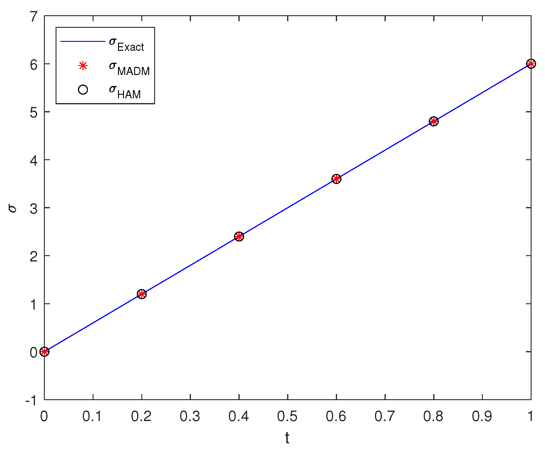
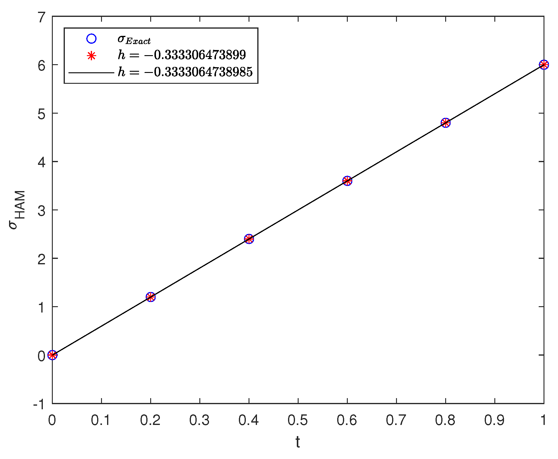
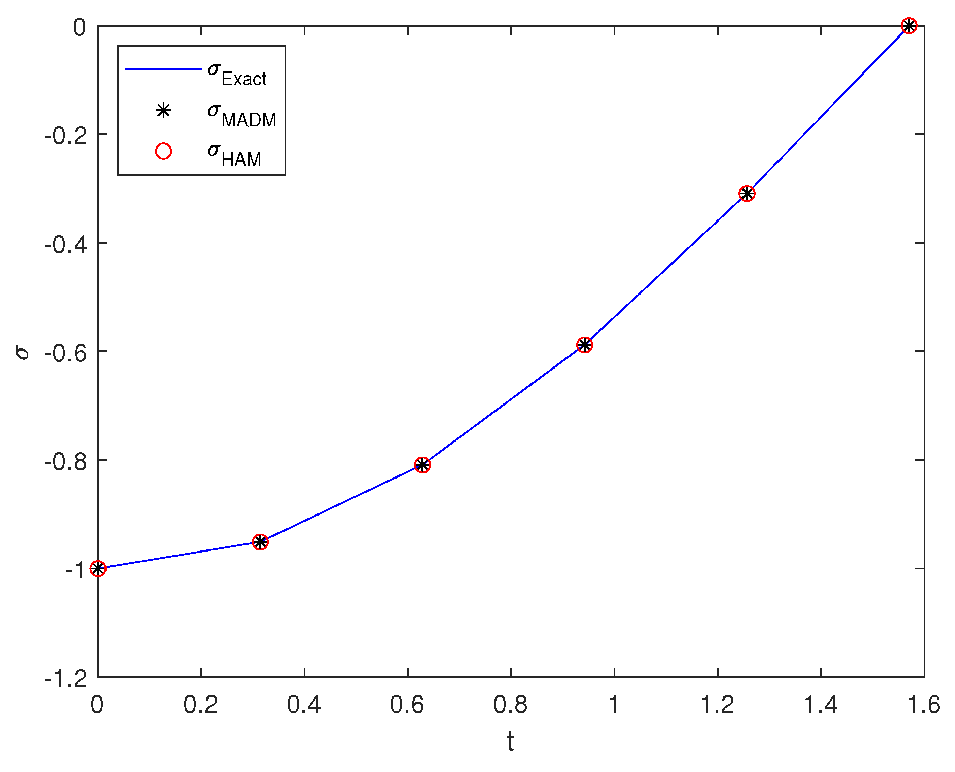
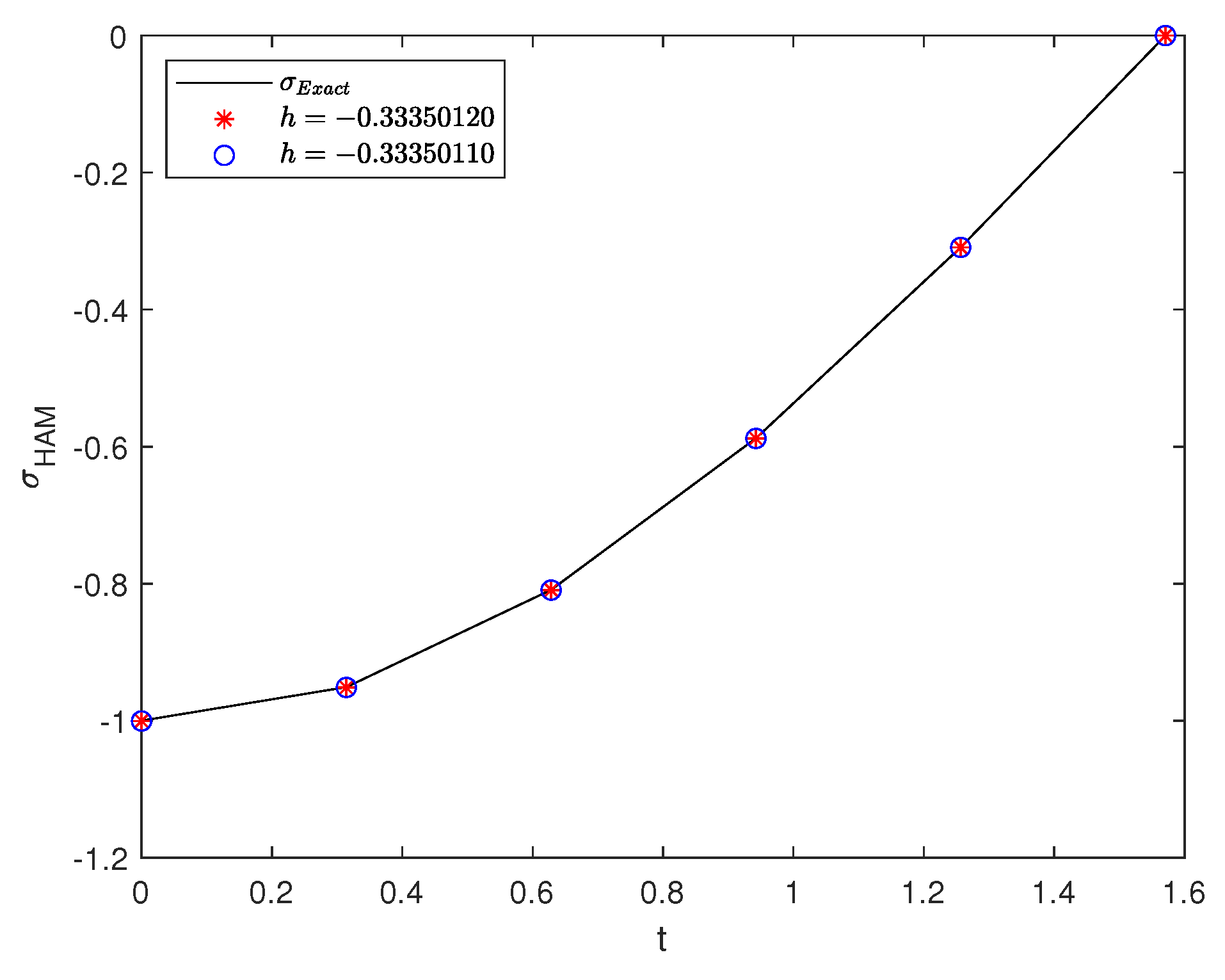
Example 1.

Our first example considers the boundary value problem

$$\mho {{\varphi }}^{″}\left(\mathtt{t}\right)+2{{\varphi }}^{\prime }\left(\mathtt{t}\right)=\mathtt{f}\left(\mathtt{t}\right)+{{\lambda }}_1{\int }_0^t\mathtt{t}(3s^2-2){{\varphi }}^3\left(s\right)ds+{{\lambda }}_2{\int }_0^1\mathtt{t}(3s^2-2){{\varphi }}^2\left(s\right)ds$$

(45)

where $\mathtt{f}\left(\mathtt{t}\right)=6\mho \mathtt{t}+6{\mathtt{t}}^2-4-{{\lambda }}_1(\frac{\mathtt{t}{({\mathtt{t}}^3-2\mathtt{t}+1)}^4}{4}-\frac{\mathtt{t}}{4})+{{\lambda }}_2\frac{\mathtt{t}}{3}$ and the exact solution ${\varphi }\left(\mathtt{t}\right)={\mathtt{t}}^3-2\mathtt{t}+1$, $\mathtt{t}\in [0,1]$ with boundary conditions ${\varphi }\left(0\right)=1,$${\varphi }\left(1\right)=0$ and $\mho =5\times {10}^3,{{\lambda }}_1=\frac{1}{300},$ and ${{\lambda }}_2=\frac{1}{400}.$ Considering the postulate $\left(\mathbf{H}\mathbf{3}\right)$,

$${\left[{\int }_0^1{\left(\mathtt{t}(3{\mathtt{y}}^2-2)\right)}^{2}d\mathtt{y}\right]}^{\frac{1}{2}}\le \frac{3}{\sqrt{5}},$$

postulate $\left(\mathbf{H}\mathbf{4}\right)$,

$$\begin{array}{cc}\hfill & \left(\xi +k_1|{{\lambda }}_1|{{\epsilon }}_1\left(1\right)+\left|{{\lambda }}_2\right|{{\epsilon }}_2\left(1\right)\right)=2.0099\le |\mho |,\hfill \\ \hfill where\xi & =2,k_1=1,\hfill \\ \hfill {{\lambda }}_1& =\frac{1}{300},{{\epsilon }}_1\left(1\right)=\frac{9}{5},\hfill \\ \hfill {{\lambda }}_2& =\frac{1}{400},{{\epsilon }}_2\left(1\right)=\frac{6}{\sqrt{15}},\hfill \end{array}$$

and postulate $\left(\mathbf{H}\mathbf{5}\right)$,

$$\begin{array}{cc}\hfill & \left(\xi +|{{\lambda }}_1|{{\Lambda }}_1+\left|{{\lambda }}_2\right|{{\Lambda }}_2\right)=2.0254\le |\mho |,\hfill \\ \hfill where\xi & =2,{{\lambda }}_1=\frac{1}{300},{{\lambda }}_2=\frac{1}{400},\hfill \\ \hfill {{\Lambda }}_1& =5.4654,{{\Lambda }}_2=2.8908,\hfill \end{array}$$

respectively. These confirm the convergence of the problem.

Repeating the above process as in Section 1 by setting $\sigma \left(\mathtt{t}\right)={{\varphi }}^{″}\left(\mathtt{t}\right)$, we can deduce a nonlinear Volterra–Fredholm integral equation in the form of (3). Moreover, (45) can satisfy the condition postulate $\left(\mathbf{H}\mathbf{5}\right)$ it has a unique solution. Thus, Theorem 8 confirms the uniqueness of solution of this problem. Finally, we tabulate the numerical results in Table 1 with $h=-0.3333064738985$ for the proposed methods and their absolute errors between them with the exact value. Moreover, we have drawn it graphically in Figure 1 for the same value of h.

Table 1. Numerical solutions for Example 1 solved by the MADM $\left({\sigma }_{MADM}\right)$ and HAM $\left({\sigma }_{HAM}\right)$.

$\mathtt{t}$	${\mathit{\sigma }}_{\mathit{exact}}$	${\mathit{\sigma }}_{\mathit{MADM}}$	${\mathit{\sigma }}_{\mathit{HAM}}$	$\parallel {\mathit{\sigma }}_{\mathit{exact}}-{\mathit{\sigma }}_{\mathit{MADM}}\parallel$	$\parallel {\mathit{\sigma }}_{\mathit{exact}}-{\mathit{\sigma }}_{\mathit{HAM}}\parallel$
0	0	0.000000000018898	−0.000266659995017	0.000000000018898	0.000266659995017
0.200000000000000	1.200000000000000	1.200000011921477	1.199658611206104	0.000000011921477	0.000341388793896
0.400000000000000	2.400000000000000	2.400000086393681	2.399647950502708	0.000000086393681	0.000352049497292
0.600000000000000	3.600000000000000	3.600000175841783	3.599701327382030	0.000000175841783	0.000298672617970
0.800000000000000	4.800000000000001	4.800000247296660	4.799818687831255	0.000000247296660	0.000181312168746
1.000000000000000	6.000000000000000	6.000000295194053	5.999999999994251	0.000000295194053	0.000000000005749

Figure 1. Plot of the proposed methods compared with the exact solution of Example 1.

For several values of $h=[-0.333306473899000-0.333306473898500-0.333306473898000]$, the best approximations of ${\sigma }_{HAM}$ can be deduced as tabulated in Table 2.

Table 2. Different values of ${\sigma }_{HAM}$ with respect to the values of $h$.

$\mathit{h}=-0.333306473899$	$\mathit{h}=-0.3333064738985$	$\mathit{h}=-0.333306473898$
−0.000266659995017	−0.000266659995017	−0.000266659995017
1.199658611207904	1.199658611206104	1.199658611204305
2.399647950506308	2.399647950502708	2.399647950499109
3.599701327387429	3.599701327382030	3.599701327376630
4.799818687838455	4.799818687831255	4.799818687824056
6.000000000003250	5.999999999994251	5.999999999985251

It is worth mentioning that the h values can confirm the convergence of the approximate solution, which are demonstrated in Figure 2.

Figure 2. ${\sigma }_{HAM}$ solutions for some values of h in Example 1.

Example 2.

Consider the following boundary value problem:

$$\mho {{\varphi }}^{″}\left(\mathtt{t}\right)=\mathtt{f}\left(\mathtt{t}\right)+{{\lambda }}_1\underset{0}{\overset{\mathtt{t}}{\int }}sin(\mathtt{t}-s){{\varphi }}^2\left(s\right)ds+{{\lambda }}_2\underset{0}{\overset{\frac{\pi }{2}}{\int }}sin(\mathtt{t}-s){\varphi }\left(s\right)ds$$

(46)

with boundary conditions

$${\varphi }\left(0\right)=1and{\varphi }\left(\frac{\pi }{2}\right)=0,$$

where $\mathtt{f}\left(\mathtt{t}\right)=-\mho cos\left(\mathtt{t}\right)-{{\lambda }}_1\left(\frac{{sin}^2\left(\mathtt{t}\right)-cos\left(\mathtt{t}\right)+1}{3}\right)-{{\lambda }}_2\left(\frac{\pi sin\left(\mathtt{t}\right)-2cos\left(\mathtt{t}\right)}{4}\right)$, ${\varphi }\left(\mathtt{t}\right)=cos\left(\mathtt{t}\right)$ is exact solution, for all $\mathtt{t}\in [0,\frac{\pi }{2}],$$\mho =4\times {10}^3,{{\lambda }}_1=\frac{1}{400}$ and ${{\lambda }}_2=\frac{1}{1200}.$

Observe that the postulate $\left(\mathbf{H}\mathbf{3}\right):$

$${\left[{\int }_0^{\frac{\pi }{2}}{\left((sin(\mathtt{t}-\mathtt{y})\right)}^{2}d\mathtt{y}\right]}^{\frac{1}{2}}\le \frac{\sqrt{\pi }}{2},$$

postulate $\left(\mathbf{H}\mathbf{4}\right):$

$$\begin{array}{cc}\hfill & \left(\xi +k_1|{{\lambda }}_1|{{\epsilon }}_1\left(1\right)+\left|{{\lambda }}_2\right|{{\epsilon }}_2\left(1\right)\right)=0.0102\le |\mho |,\hfill \\ \hfill where\xi & =0,k_1=1,\hfill \\ \hfill {{\lambda }}_1& =\frac{1}{400},{{\epsilon }}_1\left(1\right)=3.1646,\hfill \\ \hfill {{\lambda }}_2& =\frac{1}{1200},{{\epsilon }}_2\left(1\right)=2.7406,\hfill \end{array}$$

and postulate $\left(\mathbf{H}\mathbf{5}\right):$

$$\begin{array}{cc}\hfill & \left(\xi +|{{\lambda }}_1|{{\Lambda }}_1+\left|{{\lambda }}_2\right|{{\Lambda }}_2\right)=0.0260\le |\mho |,\hfill \\ \hfill where\xi & =0,{{\lambda }}_1=\frac{1}{400},{{\lambda }}_2=\frac{1}{1200},\hfill \\ \hfill {{\Lambda }}_1& =4.9093,{{\Lambda }}_2=2.7406,\hfill \end{array}$$

respectively. These confirm the convergence of the problem.

By repeating the approach described in Section 1 and setting $\sigma \left(\mathtt{t}\right):={{\varphi }}^{″}\left(\mathtt{t}\right)$, we may get a nonlinear Volterra–Fredholm integral equation in the form of (3). Furthermore, (46) meets the requirement postulate $\left(\mathbf{H}\mathbf{5}\right)$. Thus, Theorem 8 confirms the uniqueness of this problem’s solution. Finally, we arrange the numerical results for the suggested approaches and their absolute errors with the exact value in Table 3 with $h=-0.3335010$. Furthermore, we have illustrated it graphically in Figure 3 for the same value of h. Table 2 illustrates the average absolute infinity norm errors between the exact and approximate solutions (MADM and HAM) with $h=-0.3335010$.

Table 3. Numerical solutions for Example 1 solved by the MADM $\left({\sigma }_{MADM}\right)$ and HAM $\left({\sigma }_{H}AM\right)$.

$\mathtt{t}$	${\mathit{\sigma }}_{\mathit{exact}}$	${\mathit{\sigma }}_{\mathit{MADM}}$	${\mathit{\sigma }}_{\mathit{HAM}}$	$\parallel {\mathit{\sigma }}_{\mathit{Exact}}-{\mathit{\sigma }}_{\mathit{MADM}}\parallel$	$\parallel {\mathit{\sigma }}_{\mathit{Exact}}-{\mathit{\sigma }}_{\mathit{HAM}}\parallel$
0	−1.000000000000000	−1.000000843016519	−1.000503767496914	0.000000843016519	0.000503767496914
0.314159265358979	−0.951056516295154	−0.951056973274357	−0.951535349824139	0.000000456979203	0.000478833528985
0.628318530717959	−0.809016994374947	−0.809017188656542	−0.809424201820296	0.000000194281594	0.000407207445348
0.942477796076938	−0.587785252292473	−0.587785364820836	−0.588081184954149	0.000000112528363	0.000295932661675
1.256637061435917	−0.309016994374947	−0.309017207000090	−0.309172883226273	0.000000212625142	0.000155888851325
1.570796326794897	−0.000000000000000	−0.000000440291301	−0.000000736172456	0.000000440291300	0.000000736172456

Figure 3. Plot of the proposed methods compared with the exact solution of Example 2.

In addition, Figure 4 illustrates the absolute errors of infinity of the ${\sigma }_{MADM}$, $({\sigma }_{HAM}$, with $h=-0.33330490)$ and the exact solution at the same points used in Table 2.

Figure 4. ${\sigma }_{HAM}$ solutions for some values of h in Example 2.

Again, there are many values of $h=[-0.33350120-0.33350110-0.3335010]$ which give the best approximations of ${\sigma }_{HAM}$ as shown in Table 4.

Table 4. Different values of ${\sigma }_{HAM}$ with respect to the values of $h$.

$\mathit{h}=-0.33350120$	$\mathit{h}=-0.33350110$	$\mathit{h}=-0.3335010$
−1.000504367497397	−1.000504067497155	−1.000503767496914
−0.951535920505433	−0.951535635164786	−0.951535349824139
−0.809424687324857	−0.809424444572576	−0.809424201820296
−0.588081537766754	−0.588081361360451	−0.588081184954149
−0.309173068825120	−0.309172976025696	−0.309172883226273
−0.000000736408373	−0.000000736290414	−0.000000736172456

4. Conclusions and Future Directions

The main theme of this research is focused on the solution and analysis of a nonlinear boundary value problems for a Volterra–Fredholm integro equation with specific boundary conditions. We explicitly build the existence and uniqueness of an auxiliary problem with the simplified right-hand side using Arzela–Ascoli and Krasnoselskii fixed point theorems. Furthermore, using the theory of the Banach contraction principle index, we demonstrate the existence of at least one continuous solution to the original issue, as stated in Theorem 7. We have included some numerical talks and clear graphical representations for Volterra–Fredholm integro issues for several eigenvalues and homotopy parameters to help you grasp the resultant boundary models. Many solutions have been found and are depicted in Figure 1, Figure 2 and Figure 3. In addition, efficiency of the proposed schemes is also presented in tables by calculating absolute errors.

The Volterra–Fredholm integro fractional differential problems have a bright future as a type of highly integrated boundary value problem in integrated fractional operators; however, there is still room for improvement in transmission efficiency and numerical solutions, which is also the future direction of our work.

References

- AzZobi, E.; AlZoubi, W.; Akinyemi, L.; Senol, I.; Mamat, M. Abundant closed-form solitons for time-fractional integro-differential equation in fluid dynamics. Opt. Quantum Electron. 2021, 53, 132. [Google Scholar]
- Indiaminov, R.; Butaev, R.; Isayev, N.; Ismayilov, K.; Yuldoshev, B.; Numonov, A. Nonlinear integro-differential equations of bending of physically nonlinear viscoelastic plates. IOP. Conf. Ser. Mater 2020, 869, 052048. [Google Scholar] [CrossRef]
- Srivastava, H.M.; Mohammed, P.O.; Guirao, J.L.G.; Hamed, Y.S. Some higher-degree Lacunary fractional splines in the approximation of fractional differential equations. Symmetry 2021, 13, 422. [Google Scholar] [CrossRef]
- Alvarez, O.; Tourin, A. Viscosity solutions of nonlinear integro-differential equations. In Annales de l’Institut Henri Poincaré C, Analyse Non Linéaire; Elsevier: Amsterdam, The Netherlands, 1996; Volume 13, pp. 293–317. [Google Scholar]
- Laadjal, Z.; Ma, Q.-H. Existence and uniqueness of solutions for nonlinear Volterra–Fredholm integro-differential equation of fractional order with boundary conditions. J. Math. Meth. Appl. Sci. 2019, 44, 8215–8227. [Google Scholar] [CrossRef]
- Singh, H.; Sahoo, M.R.; Singh, O.P. Numerical method based on Galerkin approximation for the fractional advection-dispersion equation. Int. J. Appl. Comput. Math. 2017, 3, 2171–2187. [Google Scholar] [CrossRef]
- Rao, V.S.H.; Rao, K.K. On a nonlinear differential-integral equation for ecological problems. Bull. Austral. Math. Soc. 2009, 19, 363–369. [Google Scholar] [CrossRef]
- Hethcote, H.W.; Tudor, D.W. Integral equation models for endemic infectious diseases. J. Math. Biol. 2009, 9, 37–47. [Google Scholar] [CrossRef]
- Srivastava, H.M. A survey of some recent developments on higher transcendental functions of analytic number theory and applied mathematics. Symmetry 2021, 13, 2294. [Google Scholar] [CrossRef]
- Wazwaz, A.M.; El-Sayed, S.M. A new modification of the Adomian decomposition method for linear and nonlinear operators. J. Appl. Math. Compt. 2001, 122, 393–405. [Google Scholar] [CrossRef]
- Bildik, N.; Inc, M. Modified decomposition method for nonlinear Volterra–Fredholm integral equations. Chaos, Solit. Fract. 2007, 33, 308–313. [Google Scholar] [CrossRef]
- Abdou, M.A.; Youssef, M.I. On an approximate solution of a boundary value problem for a nonlinear integro-differential equation. Arab J. Basic Appl. Sci. 2021, 28, 386–396. [Google Scholar] [CrossRef]
- HamaRashid, H.A.; Hama, M.F. Approximate solutions for a class of nonlinear Volterra–Fredholm integro-differential equations under Dirichlet boundary conditions. AIMS Math. 2022, 8, 463–483. [Google Scholar]
- Dawooda, L.A.; Hamoud, A.A.; Mohammed, N.M. Laplace discrete decomposition method for solving nonlinear Volterra–Fredholm integro-differential equations. J. Math. Comput. Sci. 2020, 21, 158–163. [Google Scholar] [CrossRef]
- HamaRashid, H.; Srivastava, H.M.; Hama, M.; Mohammed, P.O.; Almusawa, M.Y.; Baleanu, D. Novel algorithms to approximate the solution of nonlinear integro-differential equations of Volterra-Fredholm integro type. AIMS Math. 2023, 8, 14572–14591. [Google Scholar] [CrossRef]
- Srivastava, H.M.; Saxena, R.K. Some Volterra-type fractional integro-differential equations with a multivariable confluent hypergeometric function as their kernel. J. Integr. Equat. 2005, 17, 199–217. [Google Scholar] [CrossRef]
- Diethelm, K.; Ford, J. Numerical Solution of the Bagley–Torvik Equation. BIT Numer. Math. 2002, 42, 490–507. [Google Scholar] [CrossRef]
- Wazwaz, A. A new algorithm for calculating Adomian polynomials for nonlinear operators. Appl. Math. Comput. 2000, 111, 33–51. [Google Scholar] [CrossRef]
- Babolian, E.; Biazar, J. Solution of nonlinear equations by modified Adomian decomposition method. Appl. Math. Comput. 2002, 132, 167–172. [Google Scholar] [CrossRef]
- Yalcinbas, S.; Sezer, M. The approximate solution of high-order linear Volterra–Fredholm integro-differential equations in terms of Taylor polynomials. Appl. Math. Comput. 2000, 112, 291–308. [Google Scholar]
- Batiha, B.; Noorani, M.S.M.; Hashim, I. Numerical solutions of the nonlinear integro-differential equations. IJOPCM 2008, 1, 34–42. [Google Scholar]
- El-Sayed, S.M.; Kaya, D.; Zarea, S. The decomposition method applied to solve high-order linear Volterra–Fredholm integro-differential equations. Int. J. Nonlinear Sci. Numer. Simul. 2004, 5, 105–112. [Google Scholar] [CrossRef]
- Ali, M.R.; Hadhoud, A.R.; Srivastava, H.M. Solution of fractional Volterra–Fredholm integro-differential equations under mixed boundary conditions by using the HOBW method. Adv. Differ. Equat. 2019, 2019, 115. [Google Scholar] [CrossRef]
- Ma, X.-J.; Srivastava, H.M.; Baleanu, D.; Yang, X.-J. A new Neumann series method for solving a family of local fractional Fredholm and Volterra integral equations. Math. Probl. Eng. 2013, 2013, 325121. [Google Scholar] [CrossRef]
- He, J.-H. Homotopy perturbation method: A new nonlinear analytical technique. Appl. Math. Comput. 2003, 135, 73–79. [Google Scholar] [CrossRef]
- He, J.-H. Homotopy perturbation method for solving boundary value problems. Phys. Lett. A 2006, 350, 87–88. [Google Scholar] [CrossRef]
- Liao, S. Homotopy Analysis Method in Nonlinear Differential Equations; Higher Education Press: Beijing, China; Springer: Cham, Switzerland, 2012. [Google Scholar]
- Lakshmikantham, V.; Mohana Rao, M.R. Theory of Integro-Differential Equations; Gordon and Breach Science Publishers: Amsterdam, The Netherlands, 1995. [Google Scholar]
- Mohammed, P.O.; Machado, J.A.T.; Guirao, J.L.G.; Agarwal, R.P. Adomian decomposition and fractional power series solution of a class of nonlinear fractional differential equations. Mathematics 2021, 9, 1070. [Google Scholar] [CrossRef]
- Moaaz, O.; El-Nabulsi, R.A.; Muhib, A.; Elagan, S.K.; Zakarya, M. New improved results for oscillation of fourth-order neutral differential equations. Mathematics 2021, 9, 2388. [Google Scholar] [CrossRef]
- Ali, K.K.; Mohamed, E.M.H.; Abd El salam, M.A.; Nisar, K.S.; Khashan, M.M.; Zakarya, M. A collocation approach for multiterm variable-order fractional delay-differential equations using shifted Chebyshev polynomials. Alex. Eng. J. 2022, 61, 3511–3526. [Google Scholar] [CrossRef]
- Zakarya, M.; Abd-Rabo, M.A.; AlNemer, G. Hypercomplex systems and non-Gaussian stochastic solutions with Some numerical simulation of χ-Wick-type (2 + 1)-D C-KdV equations. Axioms 2022, 11, 658. [Google Scholar] [CrossRef]
- Zhou, Y.; Wang, J.; Zhang, L. Basic Theory of Fractional Differential Equations; World Scientific: Singapore, 2016. [Google Scholar]
- Thomson, B.S.; Bruckner, J.B.; Bruckner, A.M. Elementary Real Analysis, 2nd ed.; Prentice Hall: Kent, OH, USA, 2008. [Google Scholar]
- Kilbas, A.A.; Srivastava, H.M.; Trujillo, J.J. Theory and Applications of Fractional Differential Equations; North-Holland: Amsterdam, The Netherlands; Elsevier: Amsterdam, The Netherlands, 2006. [Google Scholar]
- Smart, D.R. Fixed Point Theorem; Cambridge Tracts in Mathematics; Cambridge University Press: Cambridge, UK, 1980. [Google Scholar]
- Thomson, B. The bounded convergence theorem. Amer. Math. Mon. 2020, 127, 483–503. [Google Scholar] [CrossRef]