Computational Modeling of Individual Red Blood Cell Dynamics Using Discrete Flow Composition and Adaptive Time-Stepping Strategies

Abstract

In this article, we present a finite element method for studying the dynamic behavior of deformable vesicles, which mimic red blood cells, in a non-Newtonian Casson fluid. The fluid membrane, represented by an implicit level-set function, adheres to the Canham–Helfrich model and maintains surface inextensibility constraint through penalty. We propose a two-step time integration scheme that incorporates higher-order accuracy by using an asymmetric composition of discrete flow based on the second-order backward difference formula, followed by a projection onto the real axis. Our framework incorporates variable time steps generated by an appropriate adaptation criterion. We validate our model through numerical simulations against existing experimental and numerical results in the case of purely Newtonian flow. Furthermore, we provide preliminary results demonstrating the influence of the non-Newtonian fluid model on membrane regimes.

1. Introduction

Red blood cells (RBCs) are the primary cellular component of blood flow and play a crucial role in delivering oxygen to the body. RBCs exhibit remarkable deformability, enabling them to traverse small capillaries without rupture under high hydrodynamic stress. The dynamics of RBCs and their interactions with other blood components give rise to non-Newtonian hemorheology, particularly in small vessels and damaged blood vessels [1]. While blood can be approximated as Newtonian in large arteries with high shear rates (that is, the shear stress is proportional to the shear rate) [2], it exhibits complex non-Newtonian characteristics (e.g., shear thinning, thixotropy, yield stress, etc.) in small-diameter arteries such as capillaries and tiny arterioles [3,4,5,6]. The intricate interactions of its cellular constituents lead to significant non-Newtonian differences in its hemorheological properties, which have been extensively studied experimentally and theoretically. At low shear rates, several experimental studies have been conducted, such as the one by Cokelet in 1963 [7]. Mathematical modeling of the spatio-temporal behavior of individual RBCs is an exciting and dynamic field of research. Through modeling, we aim to gain a better understanding of the complex patterns exhibited by RBCs at the microscopic scale. Despite significant progress, the behavior of RBCs remains non-trivial, and many challenges persist [8,9,10].

We focus on performing numerical simulations of a coupled system that models the interaction between an individual RBC’s deformation and hydrodynamics using a realistic rheological model for blood at the RBC level. This modeling approach has significant importance and potential in several biomedical and therapeutic applications, such as the delivery of drugs, the treatment of cancer [11,12], and the production of biomolecules [13].

While there is growing interest in biomedical applications from the perspective of scientific computing and numerical modeling, most contributions in this field are focused on studying the dynamics of lipid vesicles in a purely Newtonian fluid. Vesicles are giant biomimetic unilamellar liposomes lacking a submembrane cytoskeleton and are commonly used as an instrumental model to study the behavior of RBCs in laboratory settings.

The mechanical properties of vesicles play a crucial role in their ability to withstand strong stresses and large deformations in flow, resulting in a wide variety of static and dynamic behaviors [14,15]. In the 1970s, Helfrich introduced a model for biomembranes where the mechanical properties are the result of bending energy minimization under constraints, also known as the Canham–Helfrich energy [16,17,18]. The bending energy density depends on the mean square curvature of the membrane. The bending force involves fourth-order derivative calculations of a shape function, which makes the problem numerically stiff and can result in several numerical difficulties [19,20,21,22].

In multiphysics modeling, there are two families of numerical strategies used for representing interfaces. Interface tracking techniques require moving meshes to track interface deformations, while interface capturing methods use fixed meshes and introduce an additional equation to implicitly track the interface [23].

The classical Galerkin finite element method [24], the boundary element method [25,26,27], the penalty-immersed boundary method [28], and the parametric finite element method [9,29] are examples of interface tracking techniques. On the other hand, the level-set method [22,30,31,32,33,34], the phase-field method [35,36], and the combined level-set and phase-field methods [37] are examples of interface capturing methods.

In this work, we use the level-set method because of the large deformations of the membrane. The level-set method has been proven effective for capturing the complex dynamics of interfaces with large deformations and topological changes [38,39,40,41].

At the microscopic scale, blood flow is characterized by the presence of aggregates of red blood cells that have a finite yield stress corresponding to a plastic solid behavior; it therefore cannot be modeled as a homogeneous Newtonian flow. Several studies have focused on the study of the non-Newtonian behavior of blood; see, for example, [42,43,44,45]. Numerous experimental studies have been performed on blood flow with different hematocrits, anticoagulants, and temperatures [46,47]. They have demonstrated that blood exhibits a finite yield strength in small vessels, owing to coagulation phenomena and the collective interactions of its components. To describe this behavior, Casson’s model has proven effective in fine-tuning experimental measurements over a range of blood vessel diameters, hematocrit levels, and shear rates [48]. We also refer to the discussion on the choice of Casson’s model for blood flow in [5]. Casson’s model expresses shear stress with respect to shear rate and a minimum yield stress [49]; see Cokelet’s work [7] for a comprehensive study. In this work, we have adopted the Casson constitutive model to describe the non-Newtonian behavior of blood at the RBC level.

As a result, blood behaves as an elastic solid at zero shear rate, when the shear stress decreases beneath the yield stress value. We often observe a change in behavior once the minimum yield limit of the fluid is exceeded [50]. However, dealing with the discontinuity of stress at a zero strain rate presents significant computational challenges. To address this challenge, various approaches have been introduced, with regularization techniques being a commonly used method. These techniques involve multiplying the stress by an exponential term [51,52,53] or simply regularizing the discontinuity at zero strain [54] in order to remove the singularity.

Given a system of differential equations obtained, for example, by finite element discretization, numerical integration using composition methods has emerged as a powerful tool for raising the order of a given lower-order basic integrator (i.e., first-order backward Euler scheme or second-order midpoint scheme) [55]. Here we introduce a technique for composing a second-order backward difference scheme, referred to as BDF-2, to increase the approximation order. This technique has been widely developed for one-step methods. For example, the Stromer–Verlet method [56], which is a symmetric and symplectic scheme used in the simulation of the Hamiltonian system [57], is the result of the composition of two schemes with a half time step: the symplectic Euler scheme (also known as the Euler–Cromer rule) [58] and its adjoint (i.e., its inverse discrete flow using a negative time step). In general, for a numerical scheme and a given time step, the composition strategy is based on multiple composition of basic numerical flows using substeps of the original time step. A theoretical framework for composition methods applied to arbitrary symmetric basic integrators was developed [59]. Various works have been carried out to build a symmetric, symplectic [59], or pseudo-numerical flow from the composition of basic discrete flows [60,61] and to increase the order of the scheme [62]. Recently, complex coefficients have been used for the composition and construction of pseudo-symplectic and pseudo-symmetric flows [63]. In particular, a time-symmetric method corresponds to its own adjoint, which represents the inverse map of the original flow with opposite time step. Symmetric methods necessarily have even orders. The composition of multi-step methods into cyclic pathways [64] has been used to improve their stability domain. This technique has been applied to solve systems, such as in electromagnetics [65], in quantum mechanics for Klein–Gordon networks [66,67], in astronomy [68], in electric and chaotic systems [69], etc. We also refer the reader to [55,62,70,71].

Furthermore, adapted time-stepping strategies can be extremely useful to better follow the dynamics of highly deformable interfaces [72,73]. The adpted step sizes can be calculated if an appropriate local error estimate is available. This could be done by considering a composition method involving complex coefficients, so that the imaginary part of the output represents an error estimate of the numerical approximation. The strategy of taking into account complex coefficients in the composition technique has been used in [63] to produce pseudo-symmetric and symplectic schemes. Recently, an error estimation of the composed Cranck–Nikolson scheme has been proposed based on the imaginary part of the composed discrete flux using complex coefficients.

For multi-step methods, the technique is more technical. Multi-step composed methods in cyclic pathways were first developed in the 1980s to improve their stability domain [64]. In this work, we develop the composition technique of the BDF-2 scheme to increase the approximation order of integration in time. Indeed, the method consists of calculating, by using the last two approximations, an intermediate value by manipulating the coefficients associated with the BDF-2 scheme. This last intermediate value is then used with the last two solutions to predict an approximation such that the new coefficients verify third-order convergence conditions. This technique will allow us to adapt the time step based on the corresponding error estimate.

The paper is organized as follows. Section 2 presents the mathematical model and describes briefly the different subproblems for a vesicle immersed in a Casson fluid. Section 3 is devoted to the time discretization and the composition technique. The numerical method is presented in Section 4. In Section 5, several numerical simulations are provided in Newtonian and non-Newtonian cases, providing better information on the accuracy of the method. We close with some conclusions and possible extensions in Section 6.

2. Mathematical Framework

The spatio-temporal deformations of the vesicle are driven by the bending force, actions of fluid forces and boundary conditions, requiring the balance equations of mass and momentum. The fluid-membrane coupling is described through the balance of hydrodynamic stress by the bending response of the membrane. The level-set description of the membrane obeys a Hamilton–Jacobi equation.

2.1. Preliminaries

By $\Lambda \subset {\mathbb{R}}^2$, we denote a given open-bounded domain with polyhedral boundary $\partial \Lambda$ and denote by $\mathit{\nu }$ the outward unit normal vector on $\partial \Lambda$. Usual notation will be adopted for Lebesgue spaces $L^p(\Omega )$ and Sobolev spaces $H^s(\Omega )$ with norm ${∥·∥}_{s,\Omega }$. For a time period $T>0$ and for any time $t\in (0,T)$, let $\Gamma \left(t\right)=\partial \Omega \left(t\right)$ represent a vesicle immersed in the domain $\Lambda$ so that $\Gamma \left(t\right)\cap \partial \Lambda =\varnothing$; $\Omega \left(t\right)$ is the inner fluid domain, while $\Lambda \in {\mathbb{R}}^2$ is the exteracellular domain. In the following, the dependence of the shape on time is omitted to lighten the notations. Let $\mathbf{n}$ and H be the unit outward normal vector and mean curvature defined for $\Gamma$, respectively. See the schematic representation in Figure 1. As usual, $\mathit{I}$ stands for the $2\times 2$ identity tensor.

Figure 1. (Left) Simulation setup of a vesicle $\Gamma =\Gamma \left(t\right)$ with enclosed fluid domain $\Omega =\Omega \left(t\right)$ immersed in an incompressible non-Newtonian fluid domain $\Lambda \backslash \Omega \left(t\right)$ under simple shear flow conditions. A band of regularization along the circumference of the vesicle is of width $2\epsilon$. (Right) Cross-section of $\Gamma$ representing a regularized sharp function $\eta$ across the membrane.

2.2. Membrane Model

Consider a vesicle freely suspended in flow. It represents a two-dimensional inextensible fluidic membrane made of two monolayers of phospholipidic molecules. To describe the mechanical properties of lipid vesicles and also provide insight into the biconcave shapes of RBCs, Canham [17], Helfrich [16], and Evans [74] independently introduced a geometric model in the early 1970s, in which the mechanical response is driven by the minimization of a bending energy density dependent on the mean squared curvature. Given a geometrical form $\Omega$ in two-dimensional space, the energy functional is given by:

$$E(\Omega )=\frac{k}{2}{\int }_{\partial \Omega }{H}^{2}ds,$$

(1)

where k is the bending rigidity modulus. The contribution of the Gaussian curvature is not relevant, if one is not interested in the change of topology; this is the case for RBCs.

We first adopt the limit of full incompressibility for both inner and outer fluids. In addition, the membrane is characterized by its local inextensibility, which forces the surface velocity divergence to vanish on the membrane. This allows it to resist stretching and leads to the preservation of the vesicle’s perimeter (or area in 3D) [75].

From a numerical point of view, the local inextensibility is generally imposed by an exact local Lagrange multiplier acting as a position-dependent membrane tension [76] or by the minimization of an elastic energy, depending on the stretching [30]. The corresponding elastic force is strongly nonlinear, which can be a source of numerical instability. As a result, fluid incompressibility and membrane inextensibility result in the preservation of global area and perimeter in 2D (or volume and surface in the 3D case). Let $\mathit{u}$ be the fluid velocity. The inextensibility constraint reads:

$${div}_s\mathit{u}=0,(0,T)\times \Gamma ,$$

(2)

where ${div}_s$ is the surface divergence operator defined through the normal $\mathbf{n}$ on the membrane. Given the generic functions f and $\mathit{v}$, the surface gradient ${\mathbf{\nabla }}_s$, the surface divergence ${div}_s$, and the Laplace–Beltrami operators ${\Delta }_s$, we write:

$$\begin{array}{cc}{\mathbf{\nabla }}_{s}f\hfill & =(\mathit{I}-\mathbf{n}\otimes \mathbf{n})\mathbf{\nabla }f,\hfill \\ {div}_s\mathit{v}\hfill & =(\mathit{I}-\mathbf{n}\otimes \mathbf{n}):\mathbf{\nabla }\mathit{v},\hfill \\ {\Delta }_{s}f\hfill & ={div}_s\left({\mathbf{\nabla }}_{s}f\right).\hfill \end{array}$$

Here, the crossed circle ⊗ represents the tensor product operator, while the semicolon : stands for the tensor contraction operator.

Based on shape optimization techniques [20], the bending force is given in the two-dimensional case by:

$$\mathit{F}=k\left({\Delta }_{s}H+\frac{H^3}{2}\right)\mathbf{n},\mathrm{on}(0,T)\times \Gamma .$$

Considering the balance of surface forces and hydrodynamic stresses acting on the vesicle, the fluid/vesicle coupling is described by the jump of the normal Cauchy stress ${\mathit{\sigma }}_{tot}$ [76]. The bending force is then transformed into a forcing surface term in the momentum equation:

$$\left[\left[{\mathit{\sigma }}_{tot}\mathbf{n}\right]\right]={\mathbf{\nabla }}_s\lambda -\lambda H\mathbf{n}+k\left({\Delta }_{s}H+\frac{H^3}{2}\right)\mathbf{n}on(0,T)\times \Gamma ,$$

where $\lambda$ stands for a local Lagrange multiplier associated with the inextensibility constraint (2).

2.3. Interface Tracking: Level-Set Representation

We use a level-set representation to follow the deformations of the vesicle $\Gamma \left(t\right)$, described in an implicit way as a zero level-set of a function $\phi$:

$$\Gamma \left(t\right)=\left\{\mathit{x}\in \Lambda ;\phi (t,\mathit{x})=0\right\}.$$

(3)

The function $\phi$ is initialized with a signed distance ${\phi }_0\left(\mathit{x}\right)$:

$${\phi }_0\left(\mathit{x}\right)=\left\{\begin{array}{c}{\displaystyle \underset{\mathit{y}\in \Gamma \left(0\right)}{inf}\parallel \mathit{y}-\mathit{x}\parallel ,\mathrm{if}\mathit{x}\notin \Omega \left(0\right)}\\ {\displaystyle -\underset{\mathit{y}\in \Gamma \left(0\right)}{inf}\parallel \mathit{y}-\mathit{x}\parallel ,\mathrm{otherwise}.}\end{array}\right.$$

All geometric fields are written in terms of $\phi$ and are extended to the entire domain $\Lambda$. In particular, $\mathbf{n}=\mathbf{\nabla }\phi /|\mathbf{\nabla }\phi |$ and $H=div\mathbf{n}$. The property of signed distance is lost by advection. To restitute the signed distance property, which is important for avoiding numerical instabilities resulting from very small or very high level-set gradients, a redistancing problem is commonly solved on a regular basis.

Surface integrals over $\Gamma$ are approximated as integrals over $\Lambda$. Set a small regularization parameter $\epsilon >0$ proportional to the mesh size. We introduce regularized Heaviside ${\mathcal{H}}_{\epsilon }$ and Dirac ${\delta }_{\epsilon }$ functions as follows:

$$\begin{array}{ccc}\hfill {\mathcal{H}}_{\epsilon }\left(\phi \right)& =& \left\{\begin{array}{cc}{\displaystyle 0,}\hfill & \mathrm{if}\phi <-\epsilon \hfill \\ {\displaystyle \frac{1}{2}\left(1+\frac{\phi }{\epsilon }+\frac{sin\left({\displaystyle \frac{\pi \phi }{\epsilon }}\right)}{\pi }\right),}\hfill & \mathrm{if}\left|\phi \right|⩽\epsilon \hfill \\ {\displaystyle 1,}\hfill & \mathrm{otherwise}\hfill \end{array}\right.,\hfill \\ \hfill {\delta }_{\epsilon }\left(\phi \right)& =& \frac{\mathrm{d}{\mathcal{H}}_{\epsilon }}{\mathrm{d}\phi }\left(\phi \right)=\left\{\begin{array}{cc}{\displaystyle \frac{1}{2\epsilon }\left(1+cos\left({\displaystyle \frac{\pi \phi }{\epsilon }}\right)\right),}\hfill & \mathrm{if}\left|\phi \right|⩽\epsilon \hfill \\ {\displaystyle 0,}\hfill & \mathrm{otherwise}\hfill \end{array}\right..\hfill \end{array}$$

For a function f and its extension $\tilde{f}$ on $\Lambda$, surface integrals are approximated as follows:

$${\int }_{\Gamma }f\left(\mathit{x}\right)d\mathit{s}\approx {\int }_{\Lambda }|\mathbf{\nabla }\phi |{\delta }_{\epsilon }\left(\phi \right)\tilde{f}\left(\mathit{x}\right)\mathrm{d}\mathit{x}.$$

(4)

The membrane force requires an evaluation of the fourth-order derivative of $\phi$, which leads to a stiff problem with strong restrictions on the time step required for stability [33,76].

2.4. Non-Newtonian Fluid Model

Let $\mathit{u}$ and p be the fluid velocity and pressure, respectively. Let $\left|\mathit{\tau }\right|={\left(\frac{1}{2}\mathit{\tau }:\mathit{\tau }\right)}^{1/2}$, with $\mathit{\tau }\in {\mathbb{R}}^{2\times 2}$ denoting the Euclidean norms of tensors. Let the positive constant ${\sigma }_0$ be the yield stress. The membrane is suspended in an incompressible non-Newtonian fluid, where the constitutive law is given by the Casson model and expresses the Cauchy stress tensor ${\mathit{\sigma }}_{tot}$ with respect to the the symmetric part of the velocity gradient (rate of deformation),

$$\mathbf{D}\left(\mathbf{u}\right)=\frac{1}{2}\left(\mathbf{\nabla }\mathit{u}+\mathbf{\nabla }{\mathit{u}}^T\right),$$

as follows:

$${\mathit{\sigma }}_{tot}=\mathit{\sigma }-p\mathbf{I}.$$

Here, $\mathit{\sigma }$ stands for the stress deviator tensor. Let $\eta (.)$ be the non-Newtonian viscosity function:

$$\begin{array}{c}\hfill \left\{\begin{array}{cc}{\displaystyle \mathit{\sigma }=2\eta \left(\left|\mathbf{D}\left(\mathbf{u}\right)\right|\right)\mathbf{D}\left(\mathbf{u}\right)={\left({\displaystyle \sqrt{K}+\sqrt{{\displaystyle \frac{{\sigma }_0}{\left|\mathbf{D}\right(\mathit{u}\left)\right|}}}}\right)}^2\mathbf{D}\left(\mathit{u}\right),}\hfill & \mathrm{when}\left|\mathbf{D}\right(\mathit{u}\left)\right|\ne 0,\hfill \\ {\displaystyle \left|\mathit{\sigma }\right|<{\sigma }_0,}\hfill & \mathrm{when}\left|\mathbf{D}\right(\mathit{u}\left)\right|=0,\hfill \end{array}\right..\end{array}$$

(5)

Here, Casson’s viscosity constant K corresponds to the fluid viscosity in the Newtonian case, that is, when the yield stress equals zero. Indeed, ${\sigma }_0=0$ reduces the constitutive equation to the Navier–Stokes case with a symmetric Cauchy stress and proportionality constant given by the constant K. Note that the stress is undetermined when $\mathbf{D}\left(\mathit{u}\right)=\mathbf{0}$, while we only know that it is less than the yield stress value. The viscosity function decreases as the shear rate increases.

According to [50], the reported yield stress values vary between $0.0002$ and $0.04$ Pa, while the Casson viscosity constant is $K\approx 0.56$ Pa·s [77]. The relation (5) is not defined when the shear rate vanishes, and one proceeds by regularization with a small positive parameter $\xi$. The limiting case $\xi \to 0$ allows us to retrieve Casson’s original model; see, for example, [52,78]. By analogy with the Newtonian case, we consider different Casson’s viscosity constants of the internal and external fluids, referred to as $K_i$ and $K_o$, respectively. Accordingly, the problem is modified in order to go back to standard equations, where the fluid behaves as a quasi-Newtonian fluid. That allows the use of standard solvers. The deviator stress in (5) writes:

$$\mathit{\sigma }=2{\eta }^{*}\left(\left|\mathbf{D}\left(\mathbf{u}\right)\right|\right)\mathbf{D}\left(\mathbf{u}\right),$$

with a viscosity function:

$$\begin{array}{c}\hfill {\eta }^{*}\left(\mathbf{D}\left(\mathit{u}\right)\right)=\left\{\begin{array}{cc}{\displaystyle \frac{1}{2}{\left(\sqrt{K_i}+\sqrt{{\displaystyle \frac{{\sigma }_0}{{\displaystyle \left|\mathbf{D}\right(\mathit{u}\left)\right|+\xi }}}}\right)}^2,}\hfill & \mathrm{in}\Omega ,\hfill \\ {\displaystyle \frac{1}{2}{\left(\sqrt{K_o}+\sqrt{{\displaystyle \frac{{\sigma }_0}{{\displaystyle \left|\mathbf{D}\right(\mathit{u}\left)\right|+\xi }}}}\right)}^2,}\hfill & \mathrm{otherwise}.\hfill \end{array}\right..\end{array}$$

(6)

To remedy the discontinuity of the viscosity accross the membrane in (6), the sharp viscosity is replaced by a smooth function:

$${\eta }_{\epsilon }^{*}(\mathbf{D}\left(\mathit{u}\right),\phi )=\frac{1}{2}{\left(\sqrt{K_o}{\mathcal{H}}_{\epsilon }\left(\phi \right)+\sqrt{K_i}\left(1-{\mathcal{H}}_{\epsilon }\left(\phi \right)\right)+\sqrt{\frac{{\sigma }_0}{\left|\mathbf{D}\right(\mathit{u}\left)\right|+\xi }}\right)}^2,\mathrm{in}\Lambda .$$

(7)

That results in a symmetric and regularized Cauchy stress tensor.

Dimensionless Nonlinear Coupled Problem

Assume a constant piecewise fluid density equal to ${\rho }_i$ and ${\rho }_o$ in the intracellular and extracellular domains, respectively. Consider a vesicle in simple shear flow as depicted in Figure 1. Opposite constant velocities $\mathit{u}=(\pm V_b,0)$ are imposed on the horizontal boundaries ${\Sigma }_D$, while stress-free boundary conditions are imposed elsewhere. Let ${\Sigma }_{-}$ denote the inflow domain. Admissible velocities belong to:

$$\mathbb{V}\left(V_b\right)=\left\{\mathbf{v}\in {\left(H^1\left(\Lambda \right)\right)}^2\mathrm{s}.\mathrm{t}.\mathbf{v}={(V_b,0)}^T\mathrm{on}{\Sigma }_D\right\}.$$

To write the dimensionless problem, we introduce some dimensionless parameters of hemodynamical relevance. Given ${\phi }_0$, the vesicle initially has a perimeter of $|\Gamma (0\left)\right|$. Set $R_0=|\Gamma \left(0\right)|/2\pi$ as the radius of a circle having the same circumference as the membrane. The confinement of the vesicle in $\Lambda$ is denoted by the dimensionless parameter $\alpha =R_0/L$. To normalize the problem, we consider the characteristic length ${\alpha }_{\mathit{x}}=L/\alpha$, the characteristic velocity ${\alpha }_{\mathit{u}}=\alpha V_b$, the characteristic time ${\alpha }_t={\alpha }_{\mathit{x}}/{\alpha }_{\mathit{u}}$, and the characteristic pressure ${\alpha }_p=R_0^2{K}_0{V}_v/L^3$. We choose ${\rho }_o$ and $K_o$ in the extracellular domain as characteristic density and viscosity, respectively.

We end up with a set of dimensionless physical parameters. The Reynolds number Re assesses inertial forces with respect to viscous forces. The bending capillary number $\mathrm{Ca}$ compares the force of the imposed flow to the membrane bending strength. Bingham’s number measures the effect of the yield stress against the rate of fluid strain. The viscosity contrast $\beta =K_i/K_o$ compares the intracellular viscosity to the extracellular viscosity in the Newtonian case. The same is true for the density contrast ${\rho }_i/{\rho }_o$. Without loss of generality, we assume similar intra- and extracellular densities as usual ${\rho }_i/{\rho }_o\approx 1$, since this parameter is known not to have an effect on the vesicle dynamics. Finally, a parameter of great importance is the reduced area; it represents the deflation of the cell which is the ratio between the enclosed area and the area of a circle having the same perimeter. The dimensionless parameters of the problem are:

$$\begin{array}{cccccc}\hfill \mathrm{Re}& =\frac{{\rho }_{o}L{V}_b}{K_o},\hfill & \hfill \mathrm{Ca}& =\frac{k{K}_o{L}^3{V}_b}{R_0},\hfill & \hfill \mathrm{Bn}& =\frac{{\sigma }_0{L}^3}{K_o{R}_0^2{V}_b},\hfill \\ \hfill {\Xi }_{2D}& =\frac{|\Omega |}{\pi }\times {\left(\frac{2\pi }{|\Gamma |}\right)}^2,\hfill & \hfill \alpha & =\frac{R_o}{L},\hfill & \hfill \beta & =\frac{K_i}{K_o}.\hfill \end{array}$$

We also refer to the work of Laadhari et al. [31,76] for a detailed description of the dimensionless problem and for obtaining the dimensionless physical parameters in the Newtonian case. In the following, all quantities are dimensionless, while the same previous notation is used. The regularization parameter is always denoted by $\xi$. The normalized problem is written as:

find φ, u, p, and λ such that                       

$$\begin{array}{ccc}\mathrm{(8a)}& \hfill \frac{\partial \phi }{\partial t}+\mathbf{u}.\mathbf{\nabla }\phi & =& 0\mathrm{in} (0,T)\times \Lambda \hfill \mathrm{(8b)}& \hfill \mathrm{Re}\left(\frac{\partial \mathbf{u}}{\partial t}+\mathbf{u}.\nabla \mathbf{u}\right)-\mathbf{div}\left(2{\eta }_{\epsilon }^{*}(\mathbf{D}\left(\mathit{u}\right),\phi )\mathbf{D}\left(\mathit{u}\right)\right)+\mathbf{\nabla }p& =& 0\mathrm{in} (0,T)\times (\Lambda \backslash \Gamma )\hfill \mathrm{(8c)}& \hfill \mathrm{div}\mathbf{u}& =& 0\mathrm{in} (0,T)\times \Lambda \hfill \mathrm{(8d)}& \hfill {\mathrm{div}}_s\mathbf{u}& =& 0\mathrm{on} (0,T)\times \Gamma \hfill \mathrm{(8e)}& \hfill \left[\right[\mathbf{u}\left]\right]& =& 0\mathrm{on} (0,T)\times \Gamma \hfill \hfill -\frac{1}{\mathrm{Ca}}\left\{{\Delta }_{s}H+\frac{H^3}{2}\right\}\mathbf{n}& & \hfill \\ \mathrm{(8f)}& \hfill +H\lambda \mathbf{n}-{\mathbf{\nabla }}_s\lambda +\left[\left[2{\eta }_{\epsilon }^{*}(\mathbf{D}\left(\mathit{u}\right),\phi )\mathbf{D}\left(\mathit{u}\right)-p\mathit{I}\right]\right].\mathbf{n}& =& 0\mathrm{on} (0,T)\times \Gamma \hfill \mathrm{(8g)}& \hfill \phi & =& {\phi }_b\mathrm{on}(0,T)\times {\Sigma }_{-}\hfill \mathrm{(8h)}& \hfill \mathbf{u}& =& {\mathbf{u}}_b\mathrm{on}(0,T)\times {\Sigma }_D\hfill \mathrm{(8i)}& \hfill (2{\eta }_{\epsilon }^{*}(\mathbf{D}\left(\mathit{u}\right),\phi )\mathbf{D}\left(\mathit{u}\right)-p\mathit{I}).\mathit{\nu }& =& 0\mathrm{on}(0,T)\times \partial \Lambda \backslash {\Sigma }_D\hfill \mathrm{(8j)}& \hfill \phi \left(0\right)& =& {\phi }_0\mathrm{in}\Lambda \hfill \mathrm{(8k)}& \hfill \mathbf{u}\left(0\right)& =& {\mathbf{u}}_0\mathrm{in}\Lambda .\hfill \end{array}$$

The normalized smooth viscosity function is:

$${\eta }_{\epsilon }^{*}(\mathbf{D}\left(\mathit{u}\right),\phi )=\frac{1}{2}{\left({\mathcal{H}}_{\epsilon }\left(\phi \right)+\sqrt{\beta }\left(1-{\mathcal{H}}_{\epsilon }\left(\phi \right)\right)+\sqrt{\frac{\mathrm{Bn}}{\left|\mathbf{D}\right(\mathit{u}\left)\right|+\xi }}\right)}^2,\mathrm{in}\Lambda .$$

(9)

3. Composition Technique Applied to the Second-Order BDF Scheme

In this section, we focus on the construction of a higher-order scheme by double composition of the second-order BDF scheme. Let us simply note the differential system obtained by finite element discretization by the following initial value problem:

$$\frac{dy}{dt}=f(t,y),y\left(0\right)=y_0,t⩾0.$$

(10)

For time interval $[0,T]$, we consider a partition into N sub-intervals $[t_n,t_{n+1})$, $n=0,\dots ,N-1$ of step size $\Delta t$. For all $n⩾1$, the unknowns $y_n$ approach the true solution $y\left(t\right)$ at discrete time steps $t_n$ and are calculated by induction. Given a numerical scheme and $n⩾1$, let ${\rm Y}$ be the numerical flow such that:

$$y_n={{\rm Y}}_{\Delta t}\left(y_{n-1}\right),\mathrm{and}\underset{n\mathrm{times}}{\underbrace{{{\rm Y}}_{\Delta t}\circ \dots \circ {{\rm Y}}_{\Delta t}\left(y_0\right)}}=y_n.$$

The numerical scheme is of order p if $y\left(t_n\right)-{{\rm Y}}_{\Delta t}\left(y_{n-1}\right)=\mathcal{O}\left(\Delta t^{p+1}\right)$. Given a basic integrator with a low order p, composition methods allow us to raise the order of the scheme by constructing a composed numerical flow ${{\rm Y}}_{a_1\Delta t}\circ \cdots \circ {{\rm Y}}_{a_s\Delta t}$, composing the basic one s times. According to [55] (Theorem 4.1, Section II.4), the composed flow is at least of order $p+1$ if and only if the coefficients $a_1,\cdots ,a_s$ verify the conditions $a_1+\dots +a_s=1$ and $a_1^{p+1}+\cdots +a_s^{p+1}=0$. For all s, these two algebraic equations have no real solution if p is odd. To construct symmetric schemes with even orders, it has been suggested to start with a second-order integrator and consider a three-times symmetric composition (i.e., $s=3$ and $a_3=a_1$) to produce the so-called triple-jump numerical flow; see, e.g., [55] (page 44) and [79]. In fact, this results from considering only symmetric compositions of second-order integrators, i.e., methods with weighting coefficients satisfying an additional condition $a_{s+1-i}=a_i$ with $i=1,\cdots ,s$. This composition has $a_2<0$, which limits its application for any non-reversible vector field. For $s=2$ and any order p, these algebraic equations have complex solutions:

$${\displaystyle a_1=\frac{1}{2}+\frac{i}{2}\frac{sin\left({\displaystyle \frac{\pi }{p+1}}\right)}{1+cos\left({\displaystyle \frac{\pi }{p+1}}\right)}\mathrm{and}{a}_2=\overline{a_1},}$$

(11)

leading to higher-order pseudo-symmetric and symplectic numerical flows [63].

Note that this technique and the choice of sub-step sizes (11) are valid for raising the orders of one-step methods, whereas this framework is not applicable to multi-step methods such as the BDF-2 method. In the following, we develop a procedure for a two-step asymmetric composition of the BDF-2 scheme using complex coefficients to both (i) increase the order of the time scheme, and also (ii) adapt the time step using the imaginary part of the compose numerical flow.

3.1. Second-Order Backward Differentiation BDF-2

For $n>1$ and given $y_{n-2}$ and $y_{n-1}$, a numerical approximation of $y\left(t_n\right)$ is computed using the BDF-2 scheme. For a constant time step $\Delta t$, the BDF-2 scheme applied to (10) approximates $y_n$ as follows:

$$3y_n-4y_{n-1}+y_{n-2}=2\Delta tf(t_n,y_n).$$

For an adaptive time step $\Delta t_n$, the difference formula rather involves some coefficients ${\gamma }_i$, with $i=0,1,2$; see, for example, [80] (Appendix G.7). The approximated solution verifies:

$${\gamma }_2{y}_n+{\gamma }_1{y}_{n-1}+{\gamma }_0{y}_{n-2}=\Delta t_{n}f(t_n,y_n),\mathrm{with}\Delta t_n=t_n-t_{n-1}.$$

This approximation can be seen as the output of the associated numerical flow, referred to as:

$$(y_n,y_{n-1})={{\rm Y}}_{\Delta t_n,{\gamma }_i}^{\mathrm{BDF}-2}(y_{n-1},y_{n-2}).$$

In what follows, we develop a technique to increase the order of BDF-2 using the double composition of the same discrete flow ${{\rm Y}}_{\Delta t_n,{\gamma }_i}^{\mathrm{BDF}-2}$ with appropriate time step and scheme coefficients. To our knowledge, the developed approach is novel for the BDF-2 scheme, while we refer to [64,81,82] for more information on the composition of multi-step methods in a cyclic way.

The method is based on computing a first approximate solution after a first jump at time $t_{n-1/2}$ using a BDF-2 method and a correctly chosen complex substep size so that the solution $y_n$ at time $t_n$ is obtained by double composition of BDF-2. A schematic representation of the extension to the complex space and two-step solution is provided in Figure 2. It can be summarized as follows:

Figure 2. Schematic representation of the BDF-2 flow composition method and the entire solution method.

Step 1:

$(y_{n-1/2},y_{n-1})={{\rm Y}}_{a_1\Delta t_n,{\gamma }_i}^{\mathrm{BDF}2}(y_{n-1},y_{n-2}),$

Step 2:

$(y_n,y_{n-1})=\mathrm{Re}\left({{\rm Y}}_{a_2\Delta t_n,{\omega }_i}^{\mathrm{BDF}2}\circ {{\rm Y}}_{a_1\Delta t_n,{\gamma }_i}^{\mathrm{BDF}2}(y_{n-1},y_{n-2})\right),$

where the parameters $a_1$, $a_2$, $\Delta t_n$, ${\gamma }_i$ and ${\omega }_i$ will be explicitly introduced in the following subsections.

3.2. Step 1: Calculation of an Intermediate Solution

For all $n>2$, consider the time steps $\Delta t_n$ so that $t_n=t_{n-1}+\Delta t_n$. Our goal is to produce a third-order approximation of $y\left(t_n\right)$ using $y_{n-2}$ and $y_{n-1}$. We first compute an intermediate step solution, denoted $y_{n-1/2}$, between $y_{n-1}$ and the desired $y_n$ using $y_{n-2}$ and $y_{n-1}$. Thus, $y_{n-1/2}\approx y\left(t_{n-1/2}\right)$ follows the BDF-2 scheme and is given by:

$${\gamma }_2{y}_{n-1/2}+{\gamma }_1{y}_{n-1}+{\gamma }_0{y}_{n-2}=(t_{n-1/2}-t_{n-1})f(t_{n-1/2},y_{n-1/2}),$$

(12)

where $t_{n-1/2}=t_{n-1}+a_1\Delta t_n$, and $a_1$ is a substep coefficient to be set subsequently. The coefficients ${\gamma }_0,{\gamma }_1$, and ${\gamma }_2$ shall satisfy:

$$y\left(t_{n-1/2}\right)-y_{n-1/2}=\mathcal{O}\left({(a_1\Delta t_n)}^3\right).$$

Note that, for a BDF scheme with a given order, the coefficients in both fixed and variable time steps do not depend obviously on the function f. We refer the interested readers to [72] (page 412, Equation (5.12)) for more details. We follow the procedure in [80] (Appendix G.7) to find the coefficients ${\gamma }_i$. Set $f(t,y)=y$, so that $y_0{e}^t$ is a solution of (10). We express $y_{n-2}$ and $y_{n-1}$ in terms of $y_{n-1/2}$:

$$y_{n-2}=e^{-(t_{n-1/2}-t_{n-2})}{y}_{n-1/2}\mathrm{and}{y}_{n-1}=e^{-(t_{n-1/2}-t_{n-1})}{y}_{n-1/2}.$$

By substituting in (12), we get:

$${\gamma }_2+{\gamma }_1{e}^{-(t_{n-1/2}-t_{n-1})}+{\gamma }_0{e}^{-(t_{n-1/2}-t_{n-2})}=t_{n-1/2}-t_{n-1}.$$

(13)

By performing Taylor series expansions in (13), we obtain:

$$\begin{array}{cc}{\gamma }_2\hfill & +{\gamma }_1\left[1-(t_{n-1/2}-t_{n-1})+\frac{1}{2}{(t_{n-1/2}-t_{n-1})}^2+\cdots \right]\hfill \\ \hfill & +{\gamma }_0\left[1-(t_{n-1/2}-t_{n-2})+\frac{1}{2}{(t_{n-1/2}-t_{n-2})}^2+\cdots \right]=t_{n-1/2}-t_{n-1}.\hfill \end{array}$$

Considering terms up to the second order gives the following linear system:

$$\begin{array}{c}\hfill \left\{{\displaystyle \begin{array}{cc}\hfill {\displaystyle {\gamma }_0+{\gamma }_1+{\gamma }_2}& =0\hfill \\ \hfill {\displaystyle {\epsilon }_n^{\prime }{\gamma }_0+{\gamma }_1+1}& =0\hfill \\ \hfill {\displaystyle {{\epsilon }_n^{\prime }}^2{\gamma }_0+{\gamma }_1}& =0\hfill \end{array}}\right.,\mathrm{with}{\epsilon }_n^{\prime }=\frac{t_{n-1/2}-t_{n-2}}{t_{n-1/2}-t_{n-1}}.\end{array}$$

(14)

The solution for the above linear system is expressed by:

$${\gamma }_0=\frac{1}{{\epsilon }_n^{\prime }({\epsilon }_n^{\prime }-1)},{\gamma }_1=-\frac{{\epsilon }_n^{\prime }}{{\epsilon }_n^{\prime }-1}\mathrm{and}{\gamma }_2=\frac{{\epsilon }_n^{\prime }+1}{{\epsilon }_n^{\prime }}.$$

(15)

As a consequence, $y_{n-1/2}$ is written as:

$$y_{n-1/2}=\frac{{\displaystyle {\gamma }_0}}{{\displaystyle (t_{n-1/2}-t_{n-1})-{\gamma }_2}}{y}_{n-2}+\frac{{\gamma }_1}{(t_{n-1/2}-t_{n-1})-{\gamma }_2}{y}_{n-1}.$$

(16)

Remark 1.

If the time steps are equally spaced, that is $\Delta t=t_{n-1}-t_{n-2}=t_{n-1/2}-t_{n-1}$, then ${\epsilon }_n^{\prime }=2$, ${\gamma }_0=1/2$, ${\gamma }_1=-4/2$, and ${\gamma }_2=3/2$. We recover the BDF-2 formula with fixed step size:

$$3y_{n-1/2}-4y_{n-1}+y_{n-2}=2\Delta tf(t_{n-1/2},y_{n-1/2}).$$

(17)

3.3. Step 2 and Solution Method

In the following, we use the three points $y_{n-2},y_{n-1}$, and $y_{n-1/2}$ to calculate an approximation $y_n$ of $y\left(t_n\right)$; see Figure 2. We define a suitable condition to eliminate $y_{n-2}$, thus using only $y_{n-1}$ and $y_{n-1/2}$ and reducing Step 2 to a two-step method to calculate $y_n$. We seek $y_n$ that satisfy the following third-order backward difference formula:

$${\omega }_2{y}_n+{\omega }_1{y}_{n-1/2}+{\omega }_0{y}_{n-1}+{\omega }_{-1}{y}_{n-2}=(t_n-t_{n-1/2})f(t_n,y_n).$$

(18)

Similar to the previous subsection, we write $y_{n-2},y_{n-1}$ in terms of $y_n$ and express $y_{n-1/2}$ using (16):

$$\begin{array}{cc}\hfill y_{n-2}& =e^{-(t_n-t_{n-2})}{y}_n,\\ \hfill y_{n-1}& =e^{-(t_n-t_{n-1})}{y}_n,\\ \hfill y_{n-1/2}& {\displaystyle =\frac{{\displaystyle {\gamma }_0{e}^{-(t_n-t_{n-2})}+{\gamma }_1{e}^{-(t_n-t_{n-1})}}}{{\displaystyle (t_{n-1/2}-t_{n-1})-{\gamma }_2}}{y}_n.}\end{array}$$

By substituting in (18), we get:

$${\displaystyle {\omega }_2+{\omega }_1\frac{{\displaystyle {\gamma }_0{e}^{-(t_n-t_{n-2})}+{\gamma }_1{e}^{-(t_n-t_{n-1})}}}{{\displaystyle (t_{n-1/2}-t_{n-1})-{\gamma }_2}}+{\omega }_0{e}^{-(t_n-t_{n-1})}+{\omega }_{-1}{e}^{-(t_n-t_{n-2})}=(t_n-t_{n-1/2}).}$$

By performing Taylor series expansions up to order 4, we obtain:

$$\begin{array}{cc}\hfill {\omega }_{-1}& ((t_{n-1/2}-t_{n-1})-{\gamma }_2)\left[1-(t_n-t_{n-2})+\frac{1}{2}{(t_n-t_{n-2})}^2-\frac{1}{6}{(t_n-t_{n-2})}^3+\cdots \right]+\hfill \\ \hfill & {\omega }_0((t_{n-1/2}-t_{n-1})-{\gamma }_2)\left[1-(t_n-t_{n-1})+\frac{1}{2}{(t_n-t_{n-1})}^2-\frac{1}{6}{(t_n-t_{n-1})}^3+\cdots \right]+\hfill \\ \hfill & {\omega }_1{\gamma }_0\left[1-(t_n-t_{n-2})+\frac{1}{2}{(t_n-t_{n-2})}^2-\frac{1}{6}{(t_n-t_{n-2})}^3+\cdots \right]+\hfill \\ \hfill & {\omega }_1{\gamma }_1\left[1-(t_n-t_{n-1})+\frac{1}{2}{(t_n-t_{n-1})}^2-\frac{1}{6}{(t_n-t_{n-1})}^3+\cdots \right]+\hfill \\ \hfill & {\omega }_2((t_{n-1/2}-t_{n-1})-{\gamma }_2)=\left((t_{n-1/2}-t_{n-1})-{\gamma }_2\right)\left(t_n-t_{n-1/2}\right).\hfill \end{array}$$

The equation can be arranged as follows:

$$\begin{array}{c}-{\omega }_{-1}{\gamma }_2-{\omega }_0{\gamma }_2+{\omega }_1({\gamma }_1+{\gamma }_2)-{\omega }_2{\gamma }_2\hfill \\ +({\omega }_{-1}+{\omega }_0+{\omega }_2)(t_{n-1/2}-t_{n-1})+({\gamma }_2{\omega }_{-1}-{\omega }_1{\gamma }_0)(t_n-t_{n-2})+({\gamma }_2{\omega }_0-{\gamma }_1{\omega }_1)(t_n-t_{n-1})\hfill \\ -\left({\omega }_{-1}(t_n-t_{n-2})+{\omega }_0(t_n-t_{n-1})\right)(t_{n-1/2}-t_{n-1})-\frac{1}{2}({\gamma }_2{\omega }_{-1}-{\omega }_1{\gamma }_0){(t_n-t_{n-2})}^2\hfill \\ -\frac{1}{2}({\gamma }_2{\omega }_0-{\gamma }_1{\omega }_1){(t_n-t_{n-1})}^2\hfill \\ +\frac{1}{2}\left({\omega }_{-1}{(t_n-t_{n-2})}^2+{\omega }_0{(t_n-t_{n-1})}^2\right)(t_{n-1/2}-t_{n-1})+\frac{1}{6}({\gamma }_2{\omega }_{-1}-{\omega }_1{\gamma }_0){(t_n-t_{n-2})}^3\hfill \\ +\frac{1}{6}({\gamma }_2{\omega }_0-{\gamma }_1{\omega }_1){(t_n-t_{n-1})}^3\hfill \\ =(t_n-t_{n-1/2})(t_{n-1/2}-t_{n-1})-{\gamma }_2(t_n-t_{n-1/2}).\hfill \end{array}$$

We identify the terms of the same power to obtain a linear system in ${\left\{{\omega }_i\right\}}_i$. To make the system easier to read, we introduce the quantities:

$$\begin{array}{cccccc}\hfill \frac{(t_{n-1/2}-t_{n-1})}{(t_n-t_{n-1})}& =a_1,\hfill & \hfill \frac{(t_n-t_{n-1/2})}{(t_n-t_{n-1})}& =1-a_1,\hfill & \hfill \frac{(t_n-t_{n-2})}{(t_n-t_{n-1})}& ={\epsilon }_n,\hfill \end{array}$$

yielding the following linear system:

$$\left\{\begin{array}{c}{\omega }_{-1}+{\omega }_0+{\omega }_1+{\omega }_2=0\hfill \\ (a_1+{\gamma }_2{\epsilon }_n){\omega }_{-1}+(a_1+{\gamma }_2){\omega }_0-({\epsilon }_n{\gamma }_0+{\gamma }_1){\omega }_1+\left(a_1\right){\omega }_2=-(1-a_1){\gamma }_2\hfill \\ (2{\epsilon }_n{a}_1+{\gamma }_2{\epsilon }_n^2){\omega }_{-1}+(2a_1+{\gamma }_2){\omega }_0-({\epsilon }_n^2{\gamma }_0+{\gamma }_1){\omega }_1=-2(1-a_1)a_1\hfill \\ (3{\epsilon }_n^2{a}_1+{\gamma }_2{\epsilon }_n^3){\omega }_{-1}+(3a_1+{\gamma }_2){\omega }_0-({\epsilon }_n^3{\gamma }_0+{\gamma }_1){\omega }_1=0.\hfill \end{array}\right.$$

For each value of $a_1$ and ${\epsilon }_n$, this system must be solved to obtain the coefficients ${\left\{{\omega }_i\right\}}_i$. By manipulating the terms, we prove that:

$${\epsilon }_n=(1-a_1)+a_1{\epsilon }_n^{\prime },\mathrm{with}{\epsilon }_n^{\prime }=1+\frac{r_n}{a_1}\mathrm{and}{r}_n=\frac{t_{n-1}-t_{n-2}}{t_n-t_{n-1}}.$$

(19)

Thus, the solution of the above system is given by:

$$\begin{array}{ccc}{\omega }_{-1}\hfill & =& {\displaystyle -\frac{(a_1-1)\left(3a_1^3+(3r_n-4)a_1^2+(r_n^2-2r_n+2)a_1+r_n\right)}{(3a_1^2+2(r_n-1)a_1-r_n)(1+r_n)r_n(a_1+r_n)}}\hfill \\ \\ {\omega }_0\hfill & =& {\displaystyle \frac{(1+r_n)(a_1-1)\left(3a_1^3+(2r_n-4)a_1^2-2(r_n-1)a_1+r_n\right)}{\left(3a_1^2+2(r_n-1)a_1-r_n\right)r_n{a}_1}}\hfill \\ \\ {\omega }_1\hfill & =& {\displaystyle -\frac{(1+r_n)(a_1-1)(2a_1+r_n)}{\left(3a_1^2+2(r_n-1)a_1-r_n\right)(a_1+r_n)a_1}}\hfill \\ \\ {\omega }_2\hfill & =& {\displaystyle -\frac{{(a_1-1)}^2((3r_n+6)a_1+2r_n^2+3r_n)}{(3a_1^2+2(r_n-1)a_1-r_n)(1+r_n)}.}\hfill \end{array}$$

(20)

Returning to the algebraic Equation (18), a fourth-order numerical approximation of $y_n$ can be obtained without using $y_{n-2}$ but provided ${\omega }_{-1}=0$. That is,

$$3a_1^3+(3r_n-4)a_1^2+(r_n^2-2r_n+2)a_1+r_n=0.$$

(21)

Solving this equation in terms of $a_1$ will help formulate the two-step composition of the BDF. Note that the trivial case $a_1=1$ causes all the coefficients ${\omega }_i=0,i=-1,0,1,2$ to vanish, thus preventing the composition from being achieved. Thereafter, we will present the composition algorithm of BDF with a fixed time step.

3.4. Algorithm of Composed BDF-2 Scheme with Fixed Time Step

Herein, the time steps $t_n$ are equidistant, which gives $r_n=1$ and ${\epsilon }_n=2$ for all $n>2$. Therefore, $a_1\ne 1$ is the solution for ${\omega }_{-1}=0$, yielding:

$$(a_1-1)(3a_1^3-a_1^2+a_1+1)=0.$$

That results in a complex step size:

$$\begin{array}{cc}\hfill a_1& =\frac{1}{9}\left({\displaystyle -\frac{8}{b}\left(\frac{1}{2}-\mathbf{i}\frac{\sqrt{3}}{2}\right)-b\left(\frac{1}{2}+\mathbf{i}\frac{\sqrt{3}}{2}\right)+1}\right),\mathrm{with}b={\left(\frac{2\sqrt{19}}{\sqrt{3}}-134\right)}^{1/3}.\hfill \end{array}$$

Hence, ${\epsilon }_n^{\prime }$, $a_2$, and the coefficients ${\gamma }_i$ from (15) are computed as follows:

$$\begin{array}{cccccccccc}\hfill {\epsilon }_n^{\prime }& =1+\frac{1}{a_1},\hfill & \hfill a_2& =1-a_1,\hfill & \hfill {\gamma }_0& =\frac{a_1^2}{a_1+1},\hfill & \hfill {\gamma }_1& =\frac{a_1+1}{a_1},\hfill & \hfill {\gamma }_2& =\frac{a_1+2}{a_1+1}.\hfill \end{array}$$

From (20), we also compute the coefficients ${\left\{{\omega }_i\right\}}_i$:

$$\begin{array}{ccc}\hfill & {\omega }_{-1}=0,\hfill & \hfill {\omega }_0=\frac{2(a_1-1)(3a_1^3-2a_1^2+1)}{(3a_1^2-1)a_1},\\ \hfill & {\omega }_1=-\frac{2(a_1-1)(2a_1+1)}{(3a_1^2-1)(a_1+1)a_1},\hfill & \hfill {\omega }_2=-\frac{{(a_1-1)}^2(9a_1+5)}{2(3a_1^2-1)}.\end{array}$$

Algorithm 1 can be summarized as follows:

Algorithm 1 Composed BDF-2 with fixed time step.

1: Set fixed-point tolerance $\mathtt{tol}$ and time step $\Delta t$   2: Set initial conditions ($n=0$): $y_0$ and $y_{-1}=y_0$   3: Compute $a_1$, ${\gamma }_i$ and ${\omega }_i$, with $i=1,2,3$   4: for $n=1,\dots ,n_{\max }$ do   5:    Update time $t_{n-1/2}=t_{n-1}+a_1\Delta t$   6:    Initialize $y_{n-1/2}^0$   7:    for $k=0,\dots ,k_{\max }$ do   8:      Compute ${\gamma }_2{y}_{n-1/2}^{k+1}+a_1\Delta tf(t_{n-1/2},y_{n-1/2}^{k+1},y_{n-1/2}^k)=-{\gamma }_1{y}_{n-1}-{\gamma }_0{y}_{n-2}$   9:      if $|y_{n-1/2}^{k+1}-y_{n-1/2}^k|<\mathtt{tol}$ then 10:         Update solution $y_{n-1/2}=y_{n-1/2}^{k+1}$ 11:         break 12:      end if 13:    end for 14:    Update time $t_n=t_{n-1/2}+a_2\Delta t$ with $a_2=1-a_1$ 15:    Initialize ${\widehat{y_n}}^0$ 16:    for $k=0,\cdots ,k_{\max }$ do 17:      Compute ${\omega }_2{\widehat{y_n}}^{k+1}+a_2\Delta t_{k}f(t_n,{\widehat{y_n}}^{k+1},{\widehat{y_n}}^k)=-{\omega }_1{y}_{n-1/2}-{\omega }_0{y}_{n-1}$ 18:      if $|{\widehat{y_n}}^{k+1}-{\widehat{y_n}}^k|<\mathtt{tol}$ then 19:         Update solution $\widehat{y_n}={\widehat{y_n}}^{k+1}$ 20:         break 21:      end if 22:    end for 23:    Set $y_n=\mathrm{Re}\left(\widehat{y_n}\right)$ as approximation of $y\left(t_n\right)$ 24:    if $t_{n+1}⩾T$ then 25:      break 26:    end if 27: end for

3.5. Algorithm for Composing BDF-2 with Adaptive Time Step

The algorithm is adapted to solve the stiff problem based on the composed BDF-2 method with adapted time steps. Its structure is similar to that presented in Algorithm 1. Nevertheless, caution is essential for calculating the parameters $a_1$, ${\gamma }_i$, and ${\omega }_i$, with $i=1,2,3$, which must now be updated at each time step.

The time step is adapted according to the imaginary part, which can represent a control criterion for the temporal integration error, as will be shown in the numerical examples. The temporal adaptation is performed in such a way that the temporal integration error does not exceed a predefined accuracy requirement TOL. For $n⩾0$ and given the order p of the integrator, the adapted time step ${\Delta t}_{n+1}$ is calculated as follows:

$$\Delta t_{n+1}=\Delta t_n\times \sqrt[p+1]{{\displaystyle \frac{\mathrm{TOL}}{C\mathrm{Im}\left(\widehat{y_n}\right)}}}$$

(22)

The algorithm is provided in Algorithm 2.

Algorithm 2 Composed BDF-2 with adaptive time steps.

1: Set fixed-point tolerance $\mathtt{tol}$, time $t=0$, and initial time step $\Delta t_1$   2: Set initial conditions: $y_0$ and $y_{-1}=y_0$   3: for $n=1,\cdots ,n_{\max }$ do   4:    Compute $r_n$ from (19) and $a_1$ from (21)   5:    Compute ${\gamma }_i$, with $i=1,2,3$ from (15)   6:    Update time $t_{n-1/2}=t_{n-1}+a_1\Delta t_n$   7:    Initialize $y_{n-1/2}^0$   8:    for $k=0,\cdots ,k_{\max }$ do   9:      Compute ${\gamma }_2{y}_{n-1/2}^{k+1}+a_1\Delta t_{n}f(t_{n-1/2},y_{n-1/2}^{k+1},y_{n-1/2}^k)=-{\gamma }_1{y}_{n-1}-{\gamma }_0{y}_{n-2}$ 10:      if $|y_{n-1/2}^{k+1}-y_{n-1/2}^k|<\mathtt{tol}$ then 11:         Update solution $y_{n-1/2}=y_{n-1/2}^{k+1}$ 12:         break 13:      end if 14:    end for 15:    Update time $t_n=t_{n-1/2}+a_2\Delta t_n$ with $a_2=1-a_1$ 16:    Compute ${\omega }_i$, with $i=1,2,3$ from (20) 17:    Initialize ${\widehat{y_n}}^0$ 18:    for $k=0,\cdots ,k_{\max }$ do 19:      Compute ${\omega }_2{\widehat{y_n}}^{k+1}+a_2\Delta t_{n}f(t_n,{\widehat{y_n}}^{k+1},{\widehat{y_n}}^k)=-{\omega }_1{y}_{n-1/2}-{\omega }_0{y}_{n-1}$ 20:      if $|{\widehat{y_n}}^{k+1}-{\widehat{y_n}}^k|<\mathtt{tol}$ then 21:         Update solution $\widehat{y_n}={\widehat{y_n}}^{k+1}$ 22:         break 23:      end if 24:    end for 25:    Set $y_n=\mathrm{Re}\left(\widehat{y_n}\right)$ as approximation of $y\left(t_n\right)$ 26:    if $t_{n+1}⩾T$ then 27:      break 28:    end if 29:    Adapt the time step $\Delta t_{n+1}$ from (22) 30: end for

4. Numerical Approximation of the Fluid/Membrane Problem

In this section, we present the main aspects of the numerical discretization. For ease of presentation, we provide the temporal discretization of both fluid and level-set problems before applying the composition technique. A penalty method is introduced to handle the surface divergence constraint, which reduces the system size and allows the use of classical Navier–Stokes solvers. The level-set problem is solved using the streamline upwind Petrov–Galerkin (SUPG) stabilization, while a fixed-point algorithm allows a tightly coupled iterative approach for the fluid/vesicle problem.

4.1. Time Discretization of the Fluid Problem

Let us divide the time interval $[0,T]$ into subintervals $[t_n,t_{n+1})$,with $n=0,\dots$ of variable time steps $\Delta t_n$. For any $n⩾0$, the unknowns ${\mathit{u}}_n$, $p_n$, and ${\phi }_n$ at time step n are iteratively computed. Semi-discrete geometric quantities and surface operators (e.g., $\mathbf{n}$, H, $\mathit{I}-\mathbf{n}\otimes \mathbf{n}$, …) at time $t_n$ are endowed with a subscript n. The semi-discretized membrane bending force at $t_n$ is written as: ${\displaystyle {\mathit{F}}_n=1/\mathrm{Ca}\left\{{\displaystyle {\Delta }_{s,n}{H}_n+H_n^3/2}\right\}{\mathbf{n}}_n}$.

Hereafter, we present the fluid problem semi-discretized in time. Without loss of generality, we assume equal densities of external and encapsulated fluids ${\rho }_i={\rho }_o$, since no dependence of densities on cellular behaviors has been observed in the literature [83]. Steps 1 and 2 of the composition algorithm both involve a second-order backward difference formula with varying time steps. Let $\delta t_n$ and ${\delta }_i$, $i=0,1,2$ represent the time step and BDF-2 coefficients, respectively; they correspond to $a_1\Delta t_n$ and ${\gamma }_i$ in Step 1 and to $a_2\Delta t_n$ and ${\omega }_i$ in Step 2. In the following, we simply present the semi-discretized problem corresponding to $(y_n,y_{n-1})={{\rm Y}}_{\delta t_n,{\delta }_i}^{\mathrm{BDF}2}(y_{n-1},y_{n-2})$.

The time derivative term of $\mathit{u}$ in the momentum equation is first discretized using a second-order backward difference formula:

$$\frac{\partial \mathit{u}}{\partial \mathrm{t}}(\mathrm{t},\mathbf{x})=\frac{{\gamma }_2\mathit{u}(\mathrm{t},\mathbf{x})+{\gamma }_1\mathit{u}(\mathrm{t}-\delta {\mathrm{t}}_n,\mathbf{x})+{\gamma }_0\mathit{u}(\mathrm{t}-2\delta {\mathrm{t}}_n,\mathbf{x})}{\delta {\mathrm{t}}_n}+\mathcal{O}\left(\delta {\mathrm{t}}_n^2\right).$$

To subsequently present the penalty approach, we also use the method of characteristics; see, e.g., [84]. For any $n>0$, let ${\mathbf{u}}^{*}=2{\mathbf{u}}_{n-1}-{\mathbf{u}}_{n-2}$ be a second-order extrapolation of $\mathbf{u}$ at time ${\mathrm{t}}_n$, with ${\mathbf{u}}_{-1}={\mathbf{u}}_0$ and ${\mathbf{u}}_{-1}$ being a convenient notation. We denote by $X_{2,n-1}$ and $X_{2,n}$ the second-order characteristics terms using the predicted ${\mathbf{u}}^{*}$. We consider a second-order approximation of the Lagrange derivative. Given an approximation of ${\phi }_n$ and ${\Gamma }_n$, the time-discretized problem (8) reads:

Find u_n, p_n, and λ_n such that:                       

$$\begin{array}{ccc}\hfill {\displaystyle \frac{Re}{\delta t_n}\left({\gamma }_2{\mathbf{u}}_n+{\gamma }_1{\mathbf{u}}_{n-1}o{X}_{2,n-1}+{\gamma }_0{\mathbf{u}}_{n-2}o{X}_{2,n-2}\right)}& & \hfill \\ \mathrm{(23a)}& \hfill -\mathbf{div}\left(2{\eta }_{\epsilon }^{*}(\mathbf{D}\left({\mathit{u}}_{n-1}\right),{\phi }_n)\mathbf{D}\left({\mathbf{u}}_n\right)\right)+\mathbf{\nabla }{p}_n& =& \mathbf{0}\mathrm{in}\Lambda \backslash \partial {\Omega }_n,\hfill \mathrm{(23b)}& \hfill \mathrm{div}{\mathbf{u}}_n& =& 0\mathrm{in}\Lambda ,\hfill \mathrm{(23c)}& \hfill {\mathrm{div}}_{s,n}{\mathbf{u}}_n& =& 0\mathrm{on}{\Gamma }_n,\hfill \mathrm{(23d)}& \hfill \left[\right[{\mathbf{u}}_n\left]\right]& =& \mathbf{0}\mathrm{on}{\Gamma }_n,\hfill \mathrm{(23e)}& \hfill \left[\right[2{\eta }_{\epsilon }^{*}\left(\mathbf{D}\left({\mathit{u}}_{n-1}\right),{\phi }_n\right)\mathbf{D}\left({\mathbf{u}}_n\right)-p_n\mathbf{I}\left]\right].{\mathbf{n}}_n-{\mathit{F}}_n+H_n{\lambda }_n{\mathbf{n}}_n-{\mathbf{\nabla }}_{s,n}{\lambda }_n& =& \mathbf{0}\mathrm{on}{\Gamma }_n,\hfill \mathrm{(23f)}& \hfill {\mathbf{u}}_n& =& {\mathbf{u}}_b\mathrm{on}{\Sigma }_D.\hfill \end{array}$$

To reduce the size of the system and allow the use of standard Navier–Stokes solvers by relaxing the constraint (23c), we present in the following subsection a penalized form of this last problem.

4.2. Penalty Method

We point out that the velocity belongs to the admissible space $\mathbb{K}\left(V\right)\cap \mathbb{L}$, with:

$$\begin{array}{cc}\hfill \mathbb{K}\left(V\right)=& \left\{\mathbf{v}\in \mathbb{V}\left(V\right)\mathrm{s}.\mathrm{t}.\mathrm{div}\mathbf{v}=0\mathrm{in}\Lambda \right\}\mathrm{and}\mathbb{L}=\left\{\mathbf{v}\in {\left(H^1\left(\Lambda \right)\right)}^2\mathrm{s}.\mathrm{t}.{\mathrm{div}}_s\mathbf{v}=0\mathrm{on}\Gamma \right\}.\hfill \end{array}$$

To remove the inextensibility (23c), we write the problem as a minimization problem:

$${\mathbf{u}}_n={\displaystyle \underset{\mathbf{v}\in \mathbb{K}(t,V_b)\cap \mathbb{L}}{\arg \inf }}{J}_n\left(\mathbf{v}\right),$$

(24)

with

$$\begin{array}{ccc}\hfill {\displaystyle J_n\left(\mathbf{v}\right)}& =& {\displaystyle \frac{Re{\gamma }_2}{2}{\int }_{\Lambda }{\mathbf{v}}^2+{\int }_{\Lambda }{\eta }_{\epsilon }^{*}(\mathbf{D}\left({\mathit{u}}_{n-1}\right),{\phi }_n){\left|2\mathbf{D}\left(\mathbf{v}\right)\right|}^2}\hfill \\ \hfill {\displaystyle }& & {\displaystyle -{\int }_{\Lambda }\left({\gamma }_1{\mathbf{u}}_{n-1}o{X}_{2,n-1}+{\gamma }_0{\mathbf{u}}_{n-2}o{X}_{2,n-2}\right)\mathbf{v}-{\int }_{{\Gamma }_n}{\mathit{F}}_n.\mathbf{v}.}\hfill \end{array}$$

We approach the minimization problem (24) with another minimization problem by penalizing the surface divergence-free condition. The membrane tension field ${\lambda }_n$ no longer appears as unknown in the problem to be solved. Let ${\epsilon }_{\lambda }$ be a small penalty parameter. The velocity field is approximated by another satisfying the penalized problem. The same notation is used for the approximate velocity, which is given by:

$${\displaystyle {\mathbf{u}}_n=\underset{\mathbf{v}\in \mathbb{K}(t,V_b)}{\arg \inf }{J}_{n,{\epsilon }_{\lambda }}\left(\mathbf{v}\right),}$$

with

$$J_{n,{\epsilon }_{\lambda }}\left(\mathbf{v}\right)=J_n\left(\mathbf{v}\right)+\frac{1}{2{\epsilon }_{\lambda }}{\int }_{{\Gamma }_n}{\left({div}_{\mathrm{s},\mathrm{n}}\mathbf{v}\right)}^2.$$

The mixed velocity/pressure formulation results from a saddle point formulation:

$$({\mathbf{u}}_n;p_n)={\displaystyle \underset{{\displaystyle \mathbf{v}\in \mathbb{V}\left(V_b\right)}}{\arg \inf }\underset{{\displaystyle \begin{array}{c}q\in L^2(\Lambda )\end{array}}}{sup}}\left\{J_{n,{\epsilon }_{\lambda }}\left(\mathit{v}\right)+{\int }_{\Lambda }q\mathrm{div}\mathit{v}\right\}.$$

The variational formulation is obtained based on the corresponding optimality conditions. After approximation of surface integrals over $\Gamma$ as integrals over the entire domain $\Lambda$, the weak formulation is given by:

find ${\mathit{u}}_n\in \mathbb{V}\left(V_b\right)$ and $p_n\in L_0^2\left(\Lambda \right)$ such that:

$$\begin{array}{ccc}& & {\displaystyle \frac{Re{\gamma }_2}{\delta t_n}{\int }_{\Lambda }{\mathit{u}}_n·\mathit{v}+{\int }_{\Lambda }2{\eta }_{\epsilon }^{*}(\mathbf{D}\left({\mathit{u}}_{n-1}\right),{\phi }_n)\mathbf{D}\left({\mathit{u}}_n\right):\mathbf{D}\left(\mathbf{v}\right)-{\int }_{\Lambda }{p}_{n}div\mathit{v}}\hfill \\ & & {\displaystyle +\frac{1}{{\epsilon }_{\lambda }}{\int }_{\Lambda }|\mathbf{\nabla }{\phi }_n|{\delta }_{\epsilon }\left({\phi }_n\right){div}_{s,n}\left({\mathit{u}}_n\right){div}_s\left(\mathit{v}\right)}\hfill \\ & & {\displaystyle ={\int }_{\Lambda }\left(|\mathbf{\nabla }{\phi }_n|{\delta }_{\epsilon }\left({\phi }_n\right){\mathit{F}}_n-{\gamma }_1{\mathbf{u}}_{n-1}o{X}_{2,n-1}-{\gamma }_0{\mathbf{u}}_{n-2}o{X}_{2,n-2}\right)·\mathit{v},\forall \mathit{v}\in \mathbb{V}\left(0\right),}\hfill \\ & & {\int }_{\Lambda }qdiv{\mathit{u}}_n=0,\forall q\in L_0^2(\Lambda ).\hfill \end{array}$$

(25)

We proceed with finite elements for the spatial discretization. Let us consider a partition ${\mathcal{T}}_h$ of $\Lambda$ consisting of geometrically conformal triangular elements K, such that ${\displaystyle \overline{\Lambda }=\underset{K\in \mathcal{T}}{\cup }}$. For any $K\in \mathcal{T}$, the mesh size h is the diameter of the largest mesh element $h=max{h}_K$. Let ${\mathsf{P}}_h^k$ be the h-dependent discrete finite element space spanned by the Lagrange polynomials of degree $k⩾1$. We consider the inf-sup stable finite element (Taylor–Hood) ${\left[{\mathsf{P}}_h^{k+1}\right]}^2-{\mathsf{P}}_h^k$ for the discretization of $\mathit{u}$ and p. The resulting nonlinear problem (25) corresponds to a classical symmetric and non-singular sparse matrix. The system is solved interatively with a preconditioned GMRES algorithm. Fixed-point iterations are also considered at each time step n to allow better numerical stability.

4.3. Level Set Problem

In a similar way, the level-set equation is discretized in time using a BDF-2 scheme. We also proceed with stabilization using the streamline upwind Petrov–Galerkin (SUPG) [85] method. In fact, we consider a classical stabilization term, denoted by $S({\tau }_K;\phi ,\psi )$, in (8a) that consists of adding some diffusion in the streamline direction. The parameter ${\tau }_K$ is the streamline diffusion coefficient that is proportional to the mesh size $h_K$ in the mesh element K and depends on the discretized velocity ${\mathit{u}}_{n,h}$. We choose:

$${\tau }_K=\frac{h_K}{s_c{\parallel {\mathit{u}}_{n,h}\parallel }_{\infty ,K}},K\in {\mathcal{T}}_h,$$

with $s_c$ a scaling factor [86]. Given ${\mathit{u}}_n$, the time-discretized level-set equation is given by:

find ${\phi }_n\in \mathbb{X}=W^{1,\infty }\left(\Lambda \right)\cap H^1\left(\Lambda \right)$ such that:

$${\int }_{\Lambda }\frac{{\gamma }_2{\phi }_n+{\gamma }_1{\phi }_{n-1}+{\gamma }_0{\phi }_{n-2}}{\delta t_n}\psi +{\int }_{\Lambda }\left({\mathit{u}}_n·\mathbf{\nabla }{\phi }_n\right)\psi +{\int }_{\Lambda }S\left({\tau }_K;{\phi }_n,\psi \right)=0,$$

(26)

for all test functions $\psi \in \mathbb{X}$. Moreover, we regularly solve for a few iterations the so-called redistancing problem, which helps to keep the level-set solution close to a signed distance function [31].

Appendix A provides additional insights into the implementation of the composition technique applied to the level set problem.

5. Numerical Results

In this section, we conduct a set of numerical experiments in the case of ordinary and partial differential equations to assess the main features of the proposed method. In Example 1, an ODE test case is presented to study both the convergence properties of the composed BDF-2 scheme and the time-stepping strategy based on the imaginary part criterion. Example 2 is dedicated to the validation of the numerical framework in terms of biophysical significance. Several validation tests are presented with comparisons to known numerical and experimental results in the published literature. Finally, in Example 3, we study the effect of non-Newtonian behavior on the membrane dynamics and present some preliminary results.

Numerical simulations have been implemented using the finite element library FEniCS [87].

5.1. Example 1: One-Dimensional Test Case—Accuracy-Order Analysis

In this example, we numerically solve the following stiff IVP using adapted time steps:

$$\begin{array}{ccc}\hfill {\displaystyle \frac{dy}{dt}}& =& y^2-y^3,t\in \left[0,\frac{2}{\varkappa }\right]\hfill \\ \hfill y\left(0\right)& =& \varkappa <1.\hfill \end{array}$$

Note that the independent variable belongs to an interval that depends on the initial value. The IVP has a known exact solution $y\left(t\right)=\frac{1}{W\left(a{e}^{a-t}\right)+1}$, where $a=\frac{1}{\varkappa }-1$ and $W\left(z\right)$ is the Lambert function defined as the solution for the equation $W{e}^W=z$. The solution starts to slowly increase from $y\left(0\right)=\varkappa$ before showing a stiff variation around $t=1/\varkappa$; it eventually reaches a stationary state $y\to 1$ when $t\to \infty$. The closer the $\varkappa$ is to zero, the steeper the curve around $t=1/\varkappa$. Figure 3 shows the exact solution for different values of the parameter $\varkappa$.

Figure 3. Graph of the exact solution of the initial value problem for different choices of the parameter $\varkappa =0.1,0.05,0.01,0.005$.

For a precise resolution, the numerical scheme must allow the use of a variable time step so that the latter is reduced when strong variations of the solution are observed, while it is increased otherwise. The time-stepping strategy could be based on an error estimate of the numerical approximation so that the time step is adapted up to a given tolerance. If the error is less than a tolerance, the step time is increased, and vice versa if not. We first compute the solution for a fixed time step equal to $\Delta t=2/640\varkappa$ to see how the imaginary part of the composed discrete flow behaves and whether this could represent an appropriate error estimate. Figure 4 plots the evolution of the error between the approximate solution, given by the real part of the composed discrete flow, and the exact solution. It also displays the imaginary part of the composed scheme. The results clearly show that both curves have the same pattern: they increase before reaching a maximum value around $t=1/\varkappa$, and they decrease afterwards.

Figure 4. Time evolution of (i) the error between the exact and computed approximate solutions $e_n=|y_n-y\left(t_n\right)|$ and (ii) the error indicator based on the imaginary part $\mathrm{Im}\left(hat{y}_n\right)$. Different values of $\varkappa =0.1,0.05,0.01,0.005$ are considered.

Consequently, the imaginary part represents a good error estimate and a precise criterion for adapting the time step size. For different parameters $\varkappa$, Figure 5 describes the adapted time steps throughout the simulation periods. The results show that the time step is correctly reduced to follow the dynamics of the solution when large variations occur in the region of stiff variations of $y_n$ with $n>0$. For $\varkappa =0.01$, we plot in the same graph the adapted time steps as well as the approximate solution and the error evolution. More importantly, Figure 6 shows the success of the method to control the error and consequently achieve the desired accuracy by adapting the time step size; the error remains less than ${10}^{-11}$.

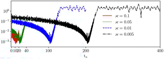
Figure 5. Evolution of the adapted time step size $\Delta t_n$ with respect to time t using the imaginary part of the composed numerical flow as an adaptation criterion. The IVP is solved for different parameters $\varkappa =0.1,0.05,0.01,0.005$.

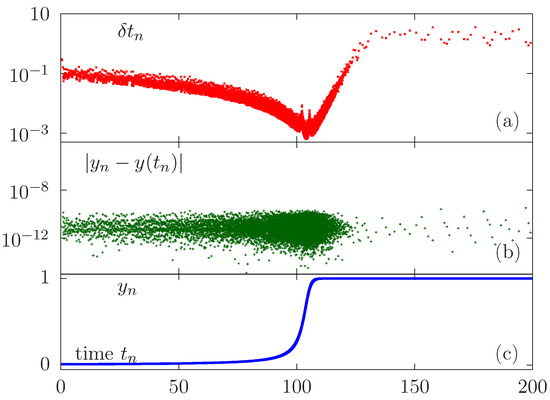
Figure 6. Quantitative study of accuracy obtained using adapted time steps. Plot of evolution in time of the time step size (a), error (b), and approximated solution (c) for $\varkappa =0.01$.

The time accuracy of the numerical approximations is studied by calculating the absolute errors for successively refined time steps compared to the exact solution. We consider the standard BDF-2 scheme and its double composition. The change in error is displayed in Figure 7, showing that optimal convergence is achieved. Convergence rates for basic and composed schemes are reported in Table 1.

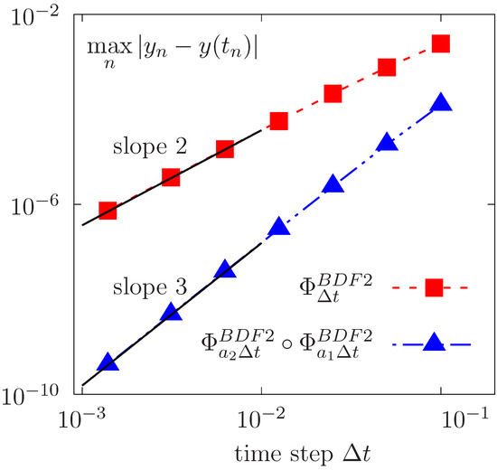
Figure 7. Temporal convergence results of the error between the exact solution and the calculated solution for different time integration methods using ${{\rm Y}}_{\Delta t}^{\mathrm{BDF}2}$ and the double flow composition ${{\rm Y}}_{a_2\Delta t}^{\mathrm{BDF}2}\circ {{\rm Y}}_{a_1\Delta t}^{\mathrm{BDF}2}$. Uniform time steps are considered.

Table 1. Table showing the error convergence rates between the exact and approximate solution in Figure 7, showing second-order and third-order for BDF-2 and its dual composition, respectively.

$1/\Delta t$	20	40	80	160	320	720
${{\rm Y}}_{\Delta t}^{\mathrm{BDF}2}$	1.65	1.83	1.92	1.96	1.98	1.99
${{\rm Y}}_{a_2\Delta t}^{\mathrm{BDF}2}\circ {{\rm Y}}_{a_1\Delta t}^{\mathrm{BDF}2}$	2.777	2.925	2.975	2.991	2.996	2.998

In the following, the time-stepping strategy will be used on a more complex PDE problem simulating the dynamics of blood cells in flow.

5.2. Example 2: Membrane Dynamics in a Newtonian Fluid under Simple Shear Flow

In this example, we perform numerical simulations of the dynamics of a two-dimensional vesicle under Newtonian shear flow. The Bingham parameter is then set to zero. A sketch of the problem setup is provided in Figure 1. We study the dynamics of a vesicle of reduced surface ${\Xi }_{2D}=0.847$ immersed in an initially stationary fluid. The membrane is confined in a square domain with confinement parameter $\alpha =1/2$. It initially has an ellipse shape, with semi-major and semi-minor axes of $\alpha /2$ and $\alpha /4$, respectively, and is located at the center of the domain; see Figure 8 (left). The physical parameters of the simulation are: $\mathrm{Re}=5.6\times {10}^{-3}$ and $\mathrm{Ca}=8\times {10}^4$. Here, we consider a uniform time step $\Delta \mathrm{t}=5\times {10}^{-3}$. Quasi-uniform unstructured meshes are generated using the mshr generator available in the FEniCS packages. Unless otherwise specified, we define ${\epsilon }_{\lambda }\approx h^{1.5}$ in our simulations, where h is the mesh size. We then provide a numerical study of the optimal choice of the penalty parameter ${\epsilon }_{\lambda }$.

Figure 8. Snapshots showing the deformations and movement of a membrane following a tank-treading regime in simple shear flow. Snapshots showing membrane deformation (red color), velocity amplitude, and streamlines. Physical parameters: ${\Xi }_{2D}=0.847$, $\beta =1$, $\mathrm{Re}=5.6\times {10}^{-3}$, $\mathrm{Ca}=8\times {10}^4$, and $\mathrm{Bn}=0$.

Under simple shear flow conditions, an inextensible two-dimensional vesicle undergoes two characteristic major dynamic behaviors known as tank-treading and tumbling regimes. For fixed physical parameters, while varying the viscosity contract between the internal fluid and the external fluid, the dynamics of the membrane change drastically. Indeed, for small viscosity ratios, the vesicle begins to rotate and reaches a stable shape with a fixed inclination angle with respect to the flow direction. The membrane continues to tank-tread around the internal fluid, which represents the tank-treading movement. By increasing the viscosity ratio above a threshold value of $\beta$, the tank-treading motion is supressed. The vesicle then behaves like a rigid elastic body that undergoes a periodic rotational movement in flow like a rigid body around its center of mass; this is the tumbling regime.

5.2.1. Tank-Treading Regime

We first set the viscosity ratio $\beta =1$. Figure 8 provides snapshots showing the dynamic behaviors of the vesicle until reaching the stationary tank-treading regime. We also plot in Figure 9 the temporal evolution of the membrane inclination angle, showing the convergence towards an equilibrium steady state. In Figure 10, we provide the variation of the relative area and relative perimeter errors throughout the simulation period, showing good conservation of area and perimeter as required by the cell model.

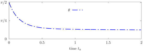
Figure 9. Time evolution of the membrane’s inclination angle for a vesicle in a tank-treading movement under simple shear flow. Physical parameters: ${\Xi }_{2D}=0.847$, $\beta =1$, $\mathrm{Re}=5.6\times {10}^{-3}$, $\mathrm{Ca}=8\times {10}^4$, and $\mathrm{Bn}=0$.

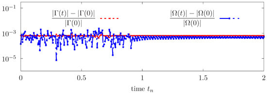
Figure 10. Time evolution of the relative error in the membrane’s area and perimeter for a vesicle in a tank-treading movement. Logarithmic scale is used on the y axis. Physical parameters: ${\Xi }_{2D}=0.847$, $\beta =1$, $\mathrm{Re}=5.6\times {10}^{-3}$, $\mathrm{Ca}=8\times {10}^4$, and $\mathrm{Bn}=0$.

Figure 11 shows the temporal evolution of the imaginary part, which is important to perform the adaptation of the time step afterwards. It can be seen that the imaginary part follows the dynamics of the membrane, where larger values are obtained as the membrane is away from the stationary tank-treading shape and begin to decrease until the equilibrium regime is reached.

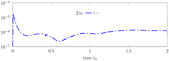
Figure 11. Error estimation based on the imaginary part throughout the simulation period for a vesicle in a tank-treading movement. Logarithmic scale is used on the y axis. Physical parameters: ${\Xi }_{2D}=0.847$, $\beta =1$, $\mathrm{Re}=5.6\times {10}^{-3}$, $\mathrm{Ca}=8\times {10}^4$, and $\mathrm{Bn}=0$.

5.2.2. Tumbling Regime

We now set a viscosity ratio $\beta =10$, resulting in a regime change towards a tumbling movement. The simulation is run for one period of complete rotation of the vesicle. Snapshots of the membrane at successive instants are provided in Figure 12.

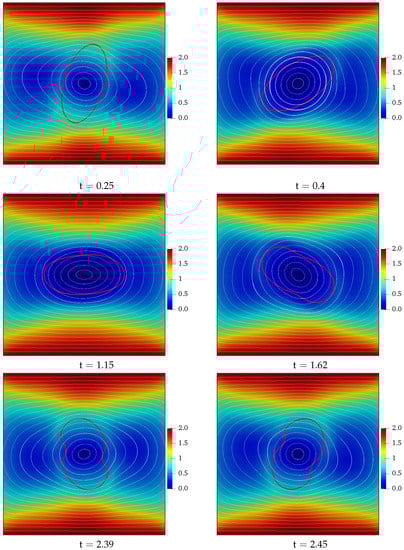
Figure 12. Tumbling motion of a vesicle immersed in a Newtonian fluid under simple shear flow. Snapshots showing membrane deformation (red color), velocity amplitude, and streamlines. Physical parameters: ${\Xi }_{2D}=0.847$, $\beta =10$, $\mathrm{Re}=5.6\times {10}^{-3}$, $\mathrm{Ca}=8\times {10}^4$, and $\mathrm{Bn}=0$.

We also provide in Figure 13 the temporal evolution of the area and perimeter, showing good conservation properties.

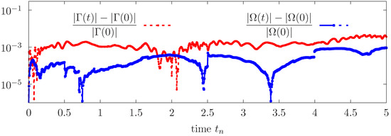
Figure 13. Time evolution of the relative error in the membrane’s area and perimeter for a vesicle in a tumbling movement. Logarithmic scale is used on the y axis. Physical parameters: ${\Xi }_{2D}=0.847$, $\beta =10$, $\mathrm{Re}=5.6\times {10}^{-3}$, $\mathrm{Ca}=8\times {10}^4$, and $\mathrm{Bn}=0$.

The angle of inclination of the membrane and the evolution over time of the imaginary part of the solution are provided respectively in Figure 14 and Figure 15. Observe that the imaginary part has four maxima during a tumbling period, which correspond to the angles of the vesicle $0,-\pi /2,-\pi ,\pi /2$. In particular, when the angle of inclination is close to $-\pi /2$ and $\pi /2$, the vesicle becomes perpendicular to the flow and undergoes a strong shearing force, inducing better tracking of the latter if the time step is sufficiently small.

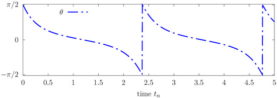
Figure 14. Time evolution of the membrane’s inclination angle for a vesicle in a tumbling movement. Physical parameters: ${\Xi }_{2D}=0.847$, $\beta =10$, $\mathrm{Re}=5.6\times {10}^{-3}$, $\mathrm{Ca}=8\times {10}^4$, and $\mathrm{Bn}=0$.

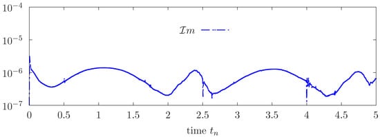
Figure 15. Error estimation based on the imaginary part throughout the simulation period for a vesicle in a tumbling movement. Logarithmic scale is used on the y axis. Physical parameters: ${\Xi }_{2D}=0.847$, $\beta =10$, $\mathrm{Re}=5.6\times {10}^{-3}$, $\mathrm{Ca}=8\times {10}^4$, and $\mathrm{Bn}=0$.

5.2.3. Calibration of the Penalty Parameter

We proceed with a numerical study to better study the setting of the penalty parameter ${\epsilon }_{\lambda }$. We consider a vesicle with a reduced area ${\Xi }_{2D}=0.85$ in simple shear flow and fix a viscosity rate of either $\beta =1$ (tank-treading motion) or $\beta =10$ (tumbling motion). The same additional parameters as the previous example are considered. We consider several values of the penalty ${\epsilon }_{\lambda }$ and evaluate in Table 2 the relative error on the perimeter. Errors are calculated over the simulation period as follows:

$$e_{|\Gamma |}={\int }_0^{\mathrm{T}}\left|\right|\Gamma \left(\mathrm{t}\right)|-|\Gamma \left(0\right)||d\mathrm{t}.$$

Table 2. Evaluation of the relative error on the perimeter of a vesicle with a reduced area ${\Xi }_{2D}=0.85$. Sensitivity study of the conservation of the perimeter with respect to the choice of ${\epsilon }_{\lambda }$. Simulations with a mesh size $h=1.7\times {10}^{-2}$.

${\mathit{\epsilon }}_{\mathit{\lambda }}$	${\mathit{h}}^1$	${\mathit{h}}^{1.2}$	${\mathit{h}}^{1.4}$	${\mathit{h}}^{1.6}$	${\mathit{h}}^{1.8}$	${\mathit{h}}^2$	${\mathit{h}}^{2.3}$
$\beta =1$	0.0022	0.021	0.0138	0.0082	0.03692	0.0512	0.0675
$\beta =10$	0.036	0.0013	0.0027	0.0057	0.0199	0.0309	0.0458

Note that the mass conservation properties are improved by decreasing the penalty parameter, up to a certain value of ${\epsilon }_{\lambda }$, beyond which the perimeter is less well preserved. Accordingly, we choose ${\epsilon }_{\lambda }=h^{1.5}$ in the following simulations.

5.2.4. Quantitative Validation with Respect to Existing Results

Subsequently, we proceed to the numerical validation of our method in the Newtonian case with some well-known results in the published literature.

Firstly, we choose the physical parameters $\beta =1$, $\mathrm{Re}={10}^{-3}$, and $\mathrm{Ca}={10}^2$. The vesicle follows a tank-treading regime, and we focus on the angle of equilibrium in the steady-state regime. A quantitative validation is performed for different reduced areas ${\Xi }_{2D}\in [0.6,0.9]$. Figure 16 shows the steady state inclination angle, denoted by ${\theta }^{*}$, obtained with different numerical methods by Laadhari et al. [76], Salac et al. [83], Kraus et al. [88], and Zhao et al. [89], as well as the experimental results provided by Kantsler and Steinberg in [90]. The numerical results show good overall agreement.

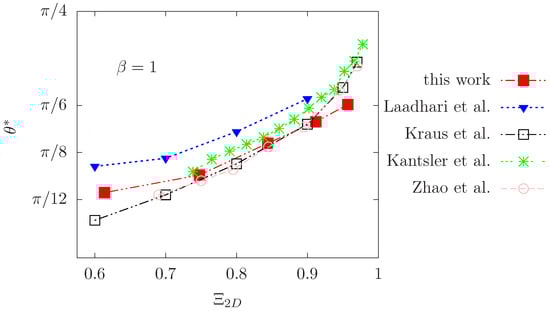
Figure 16. Vesicle under tank-treading regime in simple linear shear flow. Inclination angle at equilibrium ${\theta }^{*}$ versus the reduced area ${\Xi }_{2D}$. Physical parameters: $\beta =1$, $\mathrm{Re}={10}^{-3}$, and $\mathrm{Ca}={10}^2$. Comparisons with the published results in Laadhariet al. [76] ($\mathrm{Re}={10}^{-3}$ and $\mathrm{Ca}={10}^2$), Salac et al. [83] ($\mathrm{Re}={10}^{-3}$ and $\mathrm{Ca}={10}^2$), Kraus et al. [88] ($\mathrm{Ca}=10$), Zhao et al. [89] ($\mathrm{Ca}=9$), and the experiments of Kantsler and Steinberg [90].

Secondly, we set $\beta =2.7$ and keep the other physical parameters the same. Comparison with the numerical results of Laadhari et al. [76], Zhao et al. [89], and the experimental results in [90] are provided in Figure 17. A satisfactory agreement is observed with regard to the published data.

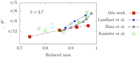
Figure 17. Vesicle following a tank-treading regime in simple linear shear flow. Angle of inclination at equilibrium ${\theta }^{*}$ with respect to the reduced area ${\Xi }_{2D}$. Physical parameters: $\beta =2.7$, $\mathrm{Re}={10}^{-3}$, and $\mathrm{Ca}={10}^2$. Comparison with the numerical results published in Laadhari et al. [76], Zhao et al. [89], and the experimental results of Kantsler and Steinberg in [90].

Finally, we are interested in the transition between tank-treading and tumbling regimes, which occurs at a threshold value of the viscosity ratio, called ${\beta }^{*}$. This is called the phase diagram. We report in Figure 18 the critical value ${\beta }^{*}$ and compare it with the results obtained from other numerical approaches in [91] (phase-field method, Re = 0), [83] (level-set method, finite difference method), [76] (level-set method, finite element method), Keller and Skalak’s theory [92], as well as the experimental results of [90]. A good qualitative and quantitative agreement is observed.

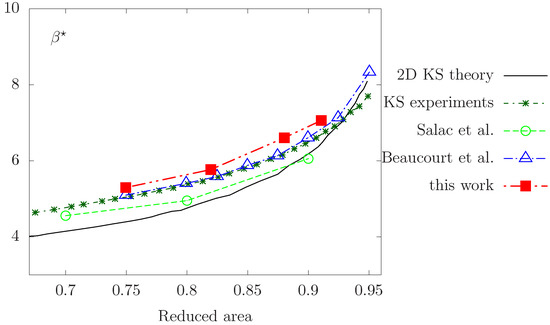
Figure 18. Phase diagram showing the critical viscosity contrast ${\beta }^{\star }$ required for the tank-treading/tumbling transition, versus the reduced area parameter ${\Xi }_{2D}$. Comparisons with numerical results in [91] (phase-field method, Stokes limit), [83] (level-set, finite difference method), [76] (level-set, finite element method), KS theory [92], and experimental results in [90].

5.3. Example 3: Membrane Dynamics in a Casson Shear Flow

In this test case, we study the effect of the Casson model on the dynamic motion of the membrane.

First, we set $\beta =1$, $\mathrm{Re}={10}^{-3}$, and $\mathrm{Ca}={10}^2$. The vesicle then follows a tank-treading motion, and we report the steady-state tilt angle in the case of a purely Newtonian fluid model as well as the change in angle when setting a non-zero Bingham parameter $\mathrm{Bn}$. We consider different reduced areas ${\Xi }_{2D}\in [0.6,0.9]$, and we set Casson’s regularization $\xi ={10}^{-2}$. The results reported in Figure 19 illustrate small changes in tilt angle for small values of $\mathrm{Bn}$, while larger changes are observed for $\mathrm{Bn}=2$.

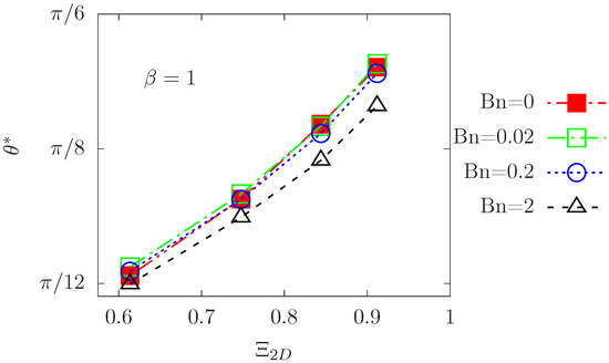
Figure 19. Numerical study of the effect of Casson flow on the vesicle tank-treading motion under simple shear flow conditions. Change in the angle of inclination at equilibrium ${\theta }^{*}$ with respect to the reduced areas ${\Xi }_{2D}$ for different values of $\mathrm{Bn}$. Simulation parameters: $\beta =1$, $\mathrm{Re}={10}^{-3}$, and $\mathrm{Ca}={10}^2$.

Now, we present a comparative study of the parameters $\beta =1$, $\mathrm{Re}={10}^{-3}$, and $\mathrm{Ca}={10}^2$, for both Newtonian and non-Newtonian cases with $Bn=2$. We observe the motion of a vesicle until it reaches a steady-state regime, undergoing tank-treading. Figure 20 displays the steady-state membrane deformations and the surrounding velocity profile for both cases. Our results indicate that a higher Bingham number leads to an inclination closer to the horizontal position.

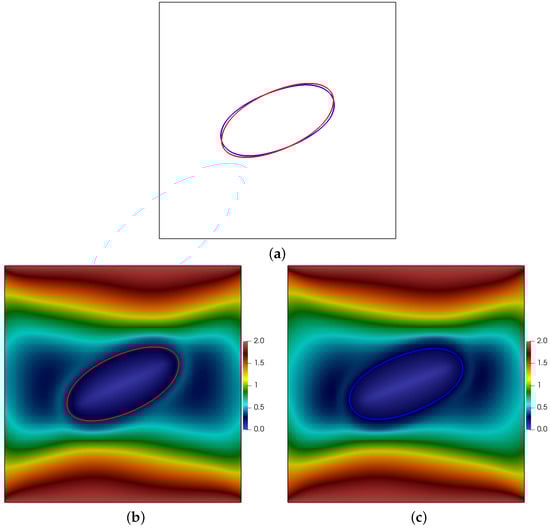
Figure 20. Change in the tank-treading stationary state between the Newtonian and non-Newtonian cases for a vesicle in simple shear flow. (a) $\mathrm{Bn}=0$ (red color), $\mathrm{Bn}=2$ (blue color). (b) Velocity profile for $\mathrm{Bn}=0$. (c) Velocity profile for $\mathrm{Bn}=2$.

We hereafter study the effect of Casson’s rheological model on the phase diagram for $\mathrm{Bn}=2$. The numerical results are reported in Figure 21, showing slightly higher values of the critical viscosity ratio needed to achieve the transition between tank-treading and tumbling regimes.

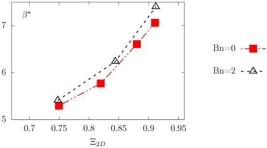
Figure 21. Numerical study of the effect of Casson flow on the transition from tank-treading to tumbling for a vesicle in simple shear flow. Changed critical viscosity contrasts ${\beta }^{*}$ against reduced areas ${\Xi }_{2D}$ for $\mathrm{Bn}=0$ and $\mathrm{Bn}=2$. Physical parameters: $\mathrm{Re}={10}^{-3}$ and $\mathrm{Ca}={10}^2$.

In conclusion, Casson’s non-Newtonian rheology should have an impact on the dynamics of red blood cells and deserves further efforts to study it. This is beyond the scope of this article, but will be deeply investigated from a biophysical point of view in future work.

6. Conclusions

We introduced a finite element methodology for the numerical simulation of inextensible biomembranes mimicking red blood cells immersed in a non-Newtonian Casson fluid. The main contributions of this article can be summarized as follows: (i) The rheological properties of blood flow in small capillaries are described by a non-Newtonian viscoplastic model through Casson’s constitutive law. To our knowledge, this is the first time that a realistic viscoplastic hemorheological model has been considered for the RBC modeling problem. (ii) Our methodology involves the introduction of the numerical integration approach based on the double-flow composition of the basic second-order backward differentiation (BDF-2) formula using complex coefficients in order to increase the order of the method. Our approach allows for an elegant estimation of the error and especially allows us to raise the order of the integrator from 2 to 3. (iii) An adaptive time-stepping strategy is introduced for higher precision in the numerical resolution. The adaptation criterion is based on a precise criterion obtained by projection of the complex approximate solution on the imaginary axis. (iv) Fluid-membrane interactions are handled implicitly through a level-set representation combined with a penalty approach. The method shows good conservation of area and perimeter (crucial issue in Eulerian methods). (v) Several numerical examples involving both ordinary and partial differential equations are performed to assess in detail the relevance of the mathematical model in terms of physiological significance. Convergence analysis is performed, showing the optimal spatio-temporal convergence behaviors. In addition, qualitative and quantitative comparative studies against analytical, numerical, and experimental results known in the published literature are carried out to validate and show the accuracy of the presented numerical approach. (vi) Preliminary study and results for the effect of the non-Newtonian rheological model on RBC regimes under simple shear flow are presented, in the hope of triggering extensive experimental and numerical studies to further explore cellular dynamics in small capillaries.

Some extensions of the developments in this article are currently being explored. In particular, the non-Newtonian effect will be explored in more detail in a separate work. This is part of a larger study of the dynamics of the biological membranes and red blood cells. We focus on developing high-precision mathematical models that better describe the mechanical properties of the cytoskeleton [32,37,93,94]. Motivated by the importance of geometric symmetries in blood flow, we will also study RBC dynamics in realistic three-dimensional axisymmetric geometries as well as flow symmetry. In a predictive modeling framework, we also plan to use the aforementioned algorithms in fluid mechanics learning with the aim of predicting the dynamics of red blood cells. We are also exploring higher-order schemes by composition of symmetric methods of order 2 and multi-step composition for various basic integrators.

References

- Connes, P.; Simmonds, M.J.; Brun, J.F.; Baskurt, O.K. Exercise hemorheology: Classical data, recent findings and unresolved issues. Clin. Hemorheol. Microcirc. 2013, 53, 187–199. [Google Scholar] [CrossRef]
- Fung, Y.C. Biomechanics, 2nd ed.; Springer: New York, NY, USA, 1993. [Google Scholar]
- Karaz, S.; Senses, E. Liposomes under Shear: Structure, Dynamics, and Drug Delivery Applications. Adv. NanoBiomed Res. 1998, 3, 2200101. [Google Scholar] [CrossRef]
- Thurston, G. Rheological parameters for the viscosity viscoelasticity and thixotropy of blood. Biorheology 1979, 16, 149–162. [Google Scholar] [CrossRef] [PubMed]
- Wajihah, S.A.; Sankar, D. A review on non-Newtonian fluid models for multi-layered blood rheology in constricted arteries. Arch. Appl. Mech. 2023, 93, 1771–1796. [Google Scholar] [CrossRef]
- Chien, S.; Usami, S.; Dellenback, R.; Gregersen, M. Shear-dependent deformation of erythrocytes in rheology of human blood. Am. J. Physiol. 1970, 219, 136–142. [Google Scholar] [CrossRef] [PubMed]
- Merrill, E.E.; Gilliland, E.R.; Cokelet, G.; Shin, H.; Britten, A.; Wells, R.E., Jr. Rheology of human blood, near and at zero flow. Effects of temperature and hematocrit level. Biophys. J. 1963, 3, 199–213. [Google Scholar] [CrossRef]
- Lai, M.C.; Li, Z. A remark on jump conditions for the three-dimensional Navier-Stokes equations involving an immersed moving membrane. Appl. Math. Lett. 2001, 14, 149–154. [Google Scholar] [CrossRef]
- Barrett, J.W.; Garcke, H.; Nurnberg, R. Numerical computations of the dynamics of fluidic membranes and vesicles. Phys. Rev. E 2015, 92, 052704. [Google Scholar] [CrossRef]
- Ayscough, S.E.; Clifton, L.A.; Skoda, M.W.; Titmuss, S. Suspended phospholipid bilayers: A new biological membrane mimetic. J. Colloid Interface Sci. 2023, 633, 1002–1011. [Google Scholar] [CrossRef]
- Noyhouzer, T.; L’Homme, C.; Beaulieu, I.; Mazurkiewicz, S.; Kuss, S.; Kraatz, H.B.; Canesi, S.; Mauzeroll, J. Ferrocene-Modified Phospholipid: An Innovative Precursor for Redox-Triggered Drug Delivery Vesicles Selective to Cancer Cells. Langmuir 2016, 32, 4169–4178. [Google Scholar] [CrossRef]
- Kaoui, B. Computer simulations of drug release from a liposome into the bloodstream. Eur. Phys. J. E 2018, 41, 20. [Google Scholar] [CrossRef] [PubMed]
- Elani, Y.; Law, R.V.; Ces, O. Vesicle-based artificial cells as chemical microreactors with spatially segregated reaction pathways. Nat. Commun. 2014, 5, 5305. [Google Scholar] [CrossRef]
- Seifert, U. Configurations of fluid membranes and vesicles. Adv. Phys. 1997, 46, 13–137. [Google Scholar] [CrossRef]
- Lipowsky, R.; Dimova, R. Introduction to remodeling of biomembranes. Soft Matter 2021, 17, 214–221. [Google Scholar] [CrossRef] [PubMed]
- Helfrich, W. Elastic properties of lipid bilayers: Theory and possible experiments. Z. Naturforschung C 1973, 28, 693–703. [Google Scholar] [CrossRef] [PubMed]
- Canham, P. The minimum energy of bending as a possible explanation of the biconcave shape of the human red blood cell. J. Theor. Biol. 1970, 26, 61–81. [Google Scholar] [CrossRef] [PubMed]
- Bassereau, P.; Sorre, B.; Lévy, A. Bending lipid membranes: Experiments after W. Helfrich’s model. Adv. Colloid Interface Sci. 2014, 208, 47–57. [Google Scholar] [CrossRef]
- Zhong-Can, O.Y.; Helfrich, W. Bending energy of vesicle membranes: General expressions for the first, second, and third variation of the shape energy and applications to spheres and cylinders. Phys. Rev. A 1989, 39, 5280–5288. [Google Scholar] [CrossRef]
- Laadhari, A.; Misbah, C.; Saramito, P. On the equilibrium equation for a generalized biological membrane energy by using a shape optimization approach. Phys. D 2010, 239, 1567–1572. [Google Scholar] [CrossRef]
- Kaoui, B.; Ristow, G.H.; Cantat, I.; Misbah, C.; Zimmermann, W. Lateral migration of a two-dimensional vesicle in unbounded Poiseuille flow. Phys. Rev. E 2008, 77, 021903. [Google Scholar] [CrossRef]
- Zhang, T.; Wolgemuth, C.W. A general computational framework for the dynamics of single- and multi-phase vesicles and membranes. J. Comput. Phys. 2022, 450, 110815. [Google Scholar] [CrossRef] [PubMed]
- Zhang, T.; Wolgemuth, C.W. Sixth-Order Accurate Schemes for Reinitialization and Extrapolation in the Level Set Framework. J. Sci. Comput. 2020, 83, 26. [Google Scholar] [CrossRef]
- Bui, C.; Lleras, V.; Pantz, O. Dynamics of red blood cells in 2d. ESAIM Proc. 2009, 28, 182–194. [Google Scholar] [CrossRef]
- Pozrikidis, C. Numerical simulation of the flow-induced deformation of red blood cells. Ann. Biomed. Eng. 2003, 31, 1194–1205. [Google Scholar] [CrossRef] [PubMed]
- Rahimian, A.; Veerapaneni, S.K.; Biros, G. Dynamic simulation of locally inextensible vesicles suspended in an arbitrary two-dimensional domain, a boundary integral method. J. Comput. Phys. 2010, 229, 6466–6484. [Google Scholar] [CrossRef]
- Dodson, W.R.; Dimitrakopoulos, P. Oscillatory tank-treading motion of erythrocytes in shear flows. Phys. Rev. E 2011, 84, 011913. [Google Scholar] [CrossRef]
- Krüger, T.; Varnik, F.; Raabe, D. Efficient and accurate simulations of deformable particles immersed in a fluid using a combined immersed boundary lattice Boltzmann finite element method. Comput. Math. Appl. 2011, 61, 3485–3505. [Google Scholar] [CrossRef]
- Bonito, A.; Nochetto, R.H.; Pauletti, M.S. Parametric FEM for geometric biomembranes. J. Comput. Phys. 2010, 229, 3171–3188. [Google Scholar] [CrossRef]
- Cottet, G.H.; Maitre, E.; Milcent, T. Eulerian formulation and Level-Set models for incompressible fluid-structure interaction. Math. Model. Numer. Anal. 2008, 42, 471–492. [Google Scholar] [CrossRef]
- Laadhari, A.; Saramito, P.; Misbah, C. Computing the dynamics of biomembranes by combining conservative level-set and adaptive finite element methods. J. Comput. Phys. 2014, 263, 328–352. [Google Scholar] [CrossRef]
- Laadhari, A. An operator splitting strategy for fluid-structure interaction problems with thin elastic structures in an incompressible Newtonian flow. Appl. Math. Lett. 2018, 81, 35–43. [Google Scholar] [CrossRef]
- Laadhari, A.; Szekely, G. Fully implicit finite element method for the modeling of free surface flows with surface tension effect. Int. J. Numer. Methods Eng. 2017, 111, 1047–1074. [Google Scholar] [CrossRef]
- Doyeux, V.; Guyot, Y.; Chabannes, V.; Prud’homme, C.; Ismail, M. Simulation of two-fluid flows using a finite element/level-set method. Application to bubbles and vesicle dynamics. J. Comput. Appl. Math. 2013, 246, 251–259. [Google Scholar] [CrossRef]
- Du, Q.; Liu, C.; Wang, X. A phase field approach in the numerical study of the elastic bending energy for vesicle membranes. J. Comput. Phys. 2004, 198, 450–468. [Google Scholar] [CrossRef]
- Valizadeh, N.; Rabczuk, T. Isogeometric analysis of hydrodynamics of vesicles using a monolithic phase-field approach. Comput. Methods Appl. Mech. Eng. 2022, 388, 114191. [Google Scholar] [CrossRef]
- Gera, P.; Salac, D. Modeling of multicomponent three-dimensional vesicles. Comput. Fluids 2018, 172, 362–383. [Google Scholar] [CrossRef]
- Osher, S.; Fedkiw, R.P. Level Set Methods: An Overview and Some Recent Results. J. Comput. Phys. 2001, 169, 463–502. [Google Scholar] [CrossRef]
- Laadhari, A. Implicit finite element methodology for the numerical modeling of incompressible two-fluid flows with moving hyperelastic interface. Appl. Math. Comput. 2018, 333, 376–400. [Google Scholar] [CrossRef]
- Laadhari, A. Exact Newton method with third-order convergence to model the dynamics of bubbles in incompressible flow. Appl. Math. Lett. 2017, 69, 138–145. [Google Scholar] [CrossRef]
- Laadhari, A.; Szekely, G. Eulerian finite element method for the numerical modeling of fluid dynamics of natural and pathological aortic valves. J. Comput. Appl. Math. 2017, 319, 236–261. [Google Scholar] [CrossRef]
- Seol, Y.; Tseng, Y.H.; Kim, Y.; Lai, M.C. An immersed boundary method for simulating Newtonian vesicles in viscoelastic fluid. J. Comput. Phys. 2019, 376, 1009–1027. [Google Scholar] [CrossRef]
- Izbassarov, D.; Muradoglu, M. A front-tracking method for computational modeling of viscoelastic two-phase flow systems. J. Non-Newton. Fluid Mech. 2015, 223, 122–140. [Google Scholar] [CrossRef]
- Suzuki, T.; Takao, H.; Suzuki, T.; Hataoka, S.; Kodama, T.; Aoki, K.; Otani, K.; Ishibashi, T.; Yamamoto, H.; Murayama, Y.; et al. Proposal of hematocrit-based non-Newtonian viscosity model and its significance in intracranial aneurysm blood flow simulation. J. Non-Newton. Fluid Mech. 2021, 290, 104511. [Google Scholar] [CrossRef]
- Gudiño, E.; Oishi, C.M.; Sequeira, A. Influence of non-Newtonian blood flow models on drug deposition in the arterial wall. J. Non-Newton. Fluid Mech. 2019, 274, 104206. [Google Scholar] [CrossRef]
- Blair, G.S. An equation for the flow of blood, plasma and serum through glass capillaries. Nature 1959, 183, 613–614. [Google Scholar] [CrossRef]
- Merrill, E.W.; Pelletier, G.A. Viscosity of human blood: Transition from Newtonian to non-Newtonian. J. Appl. Physiol. 1967, 23, 178–182. [Google Scholar] [CrossRef]
- Charm, S.; Kurland, G. Viscometry of human blood for shear rates of 0–100,000 sec−1. Nature 1965, 206, 617–618. [Google Scholar] [CrossRef]
- Casson, N. A Flow Equation for Pigment-oil Suspensions of the Printing Ink Type. In Rheology of Disperse Systems; Mills, C.C., Ed.; Pergamon Press: Oxford, UK, 1959; pp. 84–104. [Google Scholar]
- Fasano, A.; Sequeira, A. Hemomath, 1st ed.; Springer: Cham, Switzerland, 2017. [Google Scholar] [CrossRef]
- Papanastasiou, T.C. Flows of Materials with Yield. J. Rheol. 1987, 31, 385–404. [Google Scholar] [CrossRef]
- Fusi, L.; Calusi, B.; Farina, A.; Rosso, F. Stability of laminar viscoplastic flows down an inclined open channel. Eur. J. Mech. B/Fluids 2022, 95, 137–147. [Google Scholar] [CrossRef]
- Shahzad, H.; Wang, X.; Ghaffari, A.; Iqbal, K.; Hafeez, M.B.; Krawczuk, M.; Wojnicz, W. Fluid structure interaction study of non-Newtonian Casson fluid in a bifurcated channel having stenosis with elastic walls. Sci. Rep. 2022, 12, 12219. [Google Scholar] [CrossRef]
- Aghighi, M.S.; Ammar, A.; Metivier, C.; Gharagozlu, M. Rayleigh-Bénard convection of Casson fluids. Int. J. Therm. Sci. 2018, 127, 79–90. [Google Scholar] [CrossRef]
- Hairer, E.; Lubich, C.; Wanner, G. Geometric Numerical Integration: Structure-Preserving Algorithms for Ordinary Differential Equations; Springer Series in Computational Mathematics; Springer: Berlin/Heidelberg, Germany, 2002. [Google Scholar]
- Hairer, E.; Lubich, C.; Wanner, G. Geometric numerical integration illustrated by the Störmer–Verlet method. Acta Numer. 2003, 12, 399–450. [Google Scholar] [CrossRef]
- Leimkuhler, B.; Reich, S. Simulating Hamiltonian Dynamics; Cambridge Monographs on Applied and Computational Mathematics; Cambridge University Press: Cambridge, UK, 2005. [Google Scholar] [CrossRef]
- Cromer, A.H. Stable solutions using the Euler approximation. Am. J. Phys. 1981, 49, 455–459. [Google Scholar] [CrossRef]
- Yoshida, H. Construction of higher order symplectic integrators. Phys. Lett. A 1990, 150, 262–268. [Google Scholar] [CrossRef]
- McLachlan, R.I. On the Numerical Integration of Ordinary Differential Equations by Symmetric Composition Methods. SIAM J. Sci. Comput. 1995, 16, 151–168. [Google Scholar] [CrossRef]
- Blanes, S.; Casas, F.; Murua, A. Splitting and composition methods in the numerical integration of differential equations. Bol. Scc. Esp. Mat. Apl. 2008, 45, 89–145. [Google Scholar]
- Blanes, S.; Casas, F. A Concise Introduction to Geometric Numerical Integration, 1st ed.; Chapman and Hall/CRC: Boca Raton, FL, USA, 2016. [Google Scholar] [CrossRef]
- Casas, F.; Chartier, P.; Escorihuela-Tomàs, A.; Zhang, Y. Compositions of pseudo-symmetric integrators with complex coefficients for the numerical integration of differential equations. J. Comput. Appl. Math. 2021, 381, 113006. [Google Scholar] [CrossRef]
- Bickart, T.; Picel, Z. High order stiffly stable composite multistep methods for numerical integration of stiff differential equations. BIT Numer. Math. 1973, 13, 272–286. [Google Scholar] [CrossRef]
- Channell, P.J. Hybrid symplectic integrators for relativistic particles in electric and magnetic fields. Comput. Sci. Discov. 2014, 7, 015001. [Google Scholar] [CrossRef]
- Senyange, B.; Skokos, C. Computational efficiency of symplectic integration schemes: Application to multidimensional disordered Klein–Gordon lattices. Eur. Phys. J. Spec. Top. 2018, 227, 625–643. [Google Scholar] [CrossRef]
- Bader, P.; Blanes, S.; Casas, F.; Kopylov, N. Novel symplectic integrators for the Klein–Gordon equation with space- and time-dependent mass. J. Comput. Appl. Math. 2019, 350, 130–138. [Google Scholar] [CrossRef]
- Blanes, S.; Casas, F.; Farrés, A.; Laskar, J.; Makazaga, J.; Murua, A. New families of symplectic splitting methods for numerical integration in dynamical astronomy. Appl. Numer. Math. 2013, 68, 58–72. [Google Scholar] [CrossRef]
- Butusov, D.N.; Andreev, V.S.; Pesterev, D.O. Composition semi-implicit methods for chaotic problems simulation. In Proceedings of the 2016 XIX IEEE International Conference on Soft Computing and Measurements (SCM), St. Petersburg, Russia, 25–27 May 2016; pp. 107–110. [Google Scholar] [CrossRef]
- Deeb, A.; Razafindralandy, D.; Hamdouni, A. Performance of Borel-Padé-Laplace integrator for the solution of stiff and non-stiff problems. Appl. Math. Comput. 2022, 426, 127118. [Google Scholar] [CrossRef]
- Deeb, A.; Razafindralandy, D.; Hamdouni, A. Comparison between Borel-Padé summation and factorial series, as time integration methods. Discrete Contin. Dyn. Syst. Ser. S 2016, 9, 393–408. [Google Scholar] [CrossRef]
- Hairer, E.; Nørsett, S.P.; Wanner, G. Solving Ordinary Differential Equations I: Nonstiff Problems, 2nd ed.; Springer Series in Computational Mathematics Vol 1; Springer: Berlin/Heidelberg, Germany, 2009. [Google Scholar]
- Sunday, J.; Shokri, A.; Kwanamu, J.A.; Nonlaopon, K. Numerical Integration of Stiff Differential Systems Using Non-Fixed Step-Size Strategy. Symmetry 2022, 14, 1575. [Google Scholar] [CrossRef]
- Evans, E.A. Bending Resistance and Chemically Induced Moments in Membrane Bilayers. Biophys. J. 1974, 14, 923–931. [Google Scholar] [CrossRef]
- Deuling, H.; Helfrich, W. Red blood cell shapes as explained on the basis of curvature elasticity. Biophys. J. 1976, 16, 861–868. [Google Scholar] [CrossRef]
- Laadhari, A.; Saramito, P.; Misbah, C.; Székely, G. Fully implicit methodology for the dynamics of biomembranes and capillary interfaces by combining the Level Set and Newton methods. J. Comput. Phys. 2017, 343, 271–299. [Google Scholar] [CrossRef]
- Shibeshi, S.S.; Collins, W.E. The Rheology of Blood Flow in a Branched Arterial System. Appl. Rheol. 2005, 15, 398–405. [Google Scholar] [CrossRef]
- Calusi, B.; Farina, A.; Fusi, L.; Rosso, F. Long-wave instability of a regularized Bingham flow down an incline. Phys. Fluids 2022, 34, 137–147. [Google Scholar] [CrossRef]
- Suzuki, M. Fractal decomposition of exponential operators with applications to many-body theories and Monte Carlo simulations. Phys. Lett. A 1990, 146, 319–323. [Google Scholar] [CrossRef]
- Iserles, A. A First Course in the Numerical Analysis of Differential Equations, 2nd ed.; Cambridge University Press: Cambridge, UK, 2008. [Google Scholar]
- Donelson, J., III; Hansen, E. Cyclic Composite Multistep Predictor-Corrector Methods. SIAM J. Numer. Anal. 1971, 8, 137–157. [Google Scholar] [CrossRef]
- Tendler, J.M.; Bickart, T.A.; Picel, Z. A stiffly stable integration process using cyclic composite methods. ACM Trans. Math. Softw. 1978, 4, 339–368. [Google Scholar] [CrossRef]
- Salac, D.; Miksis, M. Reynolds number effects on lipid vesicles. J. Fluid Mech. 2012, 711, 122–146. [Google Scholar] [CrossRef]
- Janela, J.; Lefebvre, A.; Maury, B. A penalty method for the simulation of fluid—Rigid body interaction. ESAIM Proc. 2005, 14, 115–123. [Google Scholar] [CrossRef]
- Brooks, A.N.; Hughes, T.J. Streamline upwind/Petrov–Galerkin formulations for convection dominated flows with particular emphasis on the incompressible Navier-Stokes equations. Comput. Methods Appl. Mech. Eng. 1982, 32, 199–259. [Google Scholar] [CrossRef]
- Loch, E. The Level Set Method for Capturing Interfaces with Applications in Two-Phase Flow Problems. Ph.D. Thesis, Aachen University, Aachen, Germany, 2013. [Google Scholar]
- Alnaes, M.; Blechta, J.; Hake, J.; Johansson, A.; Kehlet, B.; Logg, A.; Richardson, C.; Ring, J.; Rognes, M.E.; Wells, G.N. The FEniCS Project Version 1.5. Arch. Numer. Softw. 2015, 3, 9–23. [Google Scholar]
- Kraus, M.; Wintz, W.; Seifert, U.; Lipowsky, R. Fluid vesicles in shear flow. Phys. Rev. Lett. 1996, 77, 3685. [Google Scholar] [CrossRef]
- Zhao, H.; Shaqfeh, E.S.G. The dynamics of a vesicle in simple shear flow. J. Fluid Mech. 2011, 674, 578–604. [Google Scholar] [CrossRef]
- Kantsler, V.; Steinberg, V. Transition to Tumbling and Two Regimes of Tumbling Motion of a Vesicle in Shear Flow. Phys. Rev. Lett. 2006, 96, 036001. [Google Scholar] [CrossRef]
- Beaucourt, J.; Rioual, F.; Séon, T.; Biben, T.; Misbah, C. Steady to unsteady dynamics of a vesicle in a flow. Phys. Rev. E 2004, 69, 011906. [Google Scholar] [CrossRef] [PubMed]
- Keller, S.R.; Skalak, R. Motion of a tank-treading ellipsoidal particle in a shear flow. J. Fluid Mech. 1982, 120, 27–47. [Google Scholar] [CrossRef]
- Laadhari, A.; Barral, Y.; Székely, G. A data-driven optimal control method for endoplasmic reticulum membrane compartmentalization in budding yeast cells. In Mathematical Methods in the Applied Sciences; Wiley Online Library: Hoboken, NJ, USA, 2023. [Google Scholar] [CrossRef]
- Gizzi, A.; Ruiz-Baier, R.; Rossi, S.; Laadhari, A.; Cherubini, C.; Filippi, S. A Three-dimensional Continuum Model of Active Contraction in Single Cardiomyocytes. In Modeling the Heart and the Circulatory System; Springer International Publishing: Cham, Switzerland, 2015; pp. 157–176. [Google Scholar] [CrossRef]
Disclaimer/Publisher’s Note: The statements, opinions and data contained in all publications are solely those of the individual author(s) and contributor(s) and not of MDPI and/or the editor(s). MDPI and/or the editor(s) disclaim responsibility for any injury to people or property resulting from any ideas, methods, instructions or products referred to in the content. |
© 2023 by the authors. Licensee MDPI, Basel, Switzerland. This article is an open access article distributed under the terms and conditions of the Creative Commons Attribution (CC BY) license (https://creativecommons.org/licenses/by/4.0/).