Abstract
In this paper, we have considered surfaces with constant negative Gaussian curvature in the simply isotropic 3-Space by defined Sauer and Strubeckerr. Firstly, we have studied the isotropic -flat, isotropic minimal and isotropic -minimal, the constant second Gaussian curvature, and the constant mean curvature of surfaces with constant negative curvature (SCNC) in the simply isotropic 3-space. Surfaces with symmetry are obtained when the mean curvatures are equal. Further, we have investigated the constant Casorati, the tangential and the amalgamatic curvatures of SCNC.
1. Introduction
Constant curvature for surfaces was one of the top subjects regarding differential geometry in the 19th century (see [1,2]). Surfaces with curvature are denoted as -surfaces, and this topic is one of the main studies in differential geometry. The hyperbolic plane’s intrinsic geometry is provided on -surfaces with a model [3,4] and the pseudosphere is the oldest known example of that geometry [5,6].
One of the most substantial problems in differential geometry is to construct a surface with constant negative Gaussian curvature in Euclidean space. From a known surface with [7], the Bäcklund’s theorem provides a geometrical method to build a family of surfaces with Gaussian curvature. For the Gaussian -surfaces, Bäcklund transformation is given by Tian [8]. For pseudospherical surfaces, Bäcklund transformation can be limited to a transformation on space curves [9]. Many studies have been conducted in other spaces, such as Minkowski space [10,11]. -surfaces in an isotropic 3-space were studied extensively by K.Strubeckerr, as in [12,13,14]. Decu and Verstraelen defined isotropic Casorati curvature [15]. Suceava investigated the tangential and amalgamatic curvatures in Euclidean 3-space [16].
Casorati proposed the Casorati curvature over Gauss and mean curvatures since this correlates better with the general intuition of curvature [16,17]. Human/computer vision and geometry are investigated using Casorati curvature [18,19]. The idea behind the amalgamatic curvature is to expand the ratio to the higher dimensions [20]. This idea can be traced back to papers [21,22], with the improvements provided in [23,24]. A recent application can be found in [16]. An important development for the invariant curvature is studied in [25] and named tangential curvature [16].
In this paper, we present the Gaussian, the second Gaussian, the mean, the second mean, the Casorati, the tangential and the amalgamatic curvatures of surfaces with a constant negative curvature defined by K.Strubeckerr and V.R.Sauer. The symmetry on the surfaces can be seen in the figures below.
2. Preliminaries
An absolute figure is an ordered triple consisting of an absolute plane w with and , which are its two complex–conjugate straight lines from the projective three-space . These are required to define the simply isotropic space , which is a Cayley–Klein space. give the absolute plane w and , are the absolute lines , . They are called the homogeneous coordinates or projective coordinates in [26]. Homogeneous coordinates played an important role in capturing the projection of a 3D view for use in monitors, T.V., etc. [27] Further information about Cayley–Klein spaces can be acquired from [28].
The absolute point is defined as the crossing node of these two lines. A motion in is a given with corresponding coordinates, as can be found at [26] and given as
where . These are named isotropic congruence transformations [26]. Isotropic congruence transformations looks like Euclidean motions (combination of a translation and a rotation) in the projection onto the xy-plane. This projection is named as a “top view” [29,30,31]. The combination of a Euclidean motion in the xy-plane and affine transformation with shearing along the z-direction is called an isotropic motion [32].
The equation
is defined as the metric of . Let U = and V = be vectors in ; then, the inner product of U and V is defined as,
This metric is induced by the absolute figure. If a line is not parallel to the z-direction, it is called non-isotropic; otherwise, it is isotropic. Isotropic planes are the planes that contain an isotropic line. Consider a -surface , , in parameterized by
Let an arbitrary surface in be called . If a surface has no isotropic tangent planes, then it is called an admissible surface. The first and second forms and , called fundamental forms, of , have the coefficients and , respectively, which can be easily stated with the induced matrix, given by [32] as,
where (with )
Then, and , the isotropic Gaussian curvature and mean curvature, can be defined as
where are principal curvatures.Therefore, the extrema of the normal curvatures, and , are determined with the non-isotropic section of the surface. Here, when and the surfaces are called, respectively, isotropic flat and isotropic minimal [26]. Isotropic -flat and isotropic -minimal are named after the moment when a non-developable surface’s second Gaussian curvature and second mean curvature are zero, respectively. The second Gaussian curvature of is given by
The second mean curvature for a surface in simply isotropic 3-space is given by [15]
where , and is the inverse of the matrix of the second fundamental form [33]. The isotropic Casorati curvature is defined by
The tangential curvature and the amalgamatic curvature are given by
respectively [16].
3. Curvatures of SCNC in
In this chapter, we provide the curvatures of SCNC in . The general form of SCNC can be derived as follows. Let be a surface with
when we have
where with and are twice continuous differentiable functions of u and v, respectively. The parametric curves are asymptotic if and only if the two conditions
are fulfilled. From the above equations with condition, the existence of two functions and can be uniquely determined by , which satisfy the equations
By solving these equations, we can obtained
For the arbitrary functions , from the solution of the previous equation, we obtain,
results in
Then,
by choosing
we obtain
by using these in the equations,
The integrability condition is fulfilled and, from integration, results in , from this, , we can obtained as
where are functions of u and are functions of v [12,34]. The isotropic curvature and the mean curvature of the surface (8) is given by
Assume the mean curvature of (8) is constant. Then,
where If we use the separation of variables method, the mean curvature and the mean curvature if and only if
where are independent variables and both sides of the Equation (10) are constant. If we show that this constant is equal to p, we can obtain
Hence, we can write
where
If the surface (8) is isotropic minimal, then, from (10), we have
and as a result of the solution of this equation,
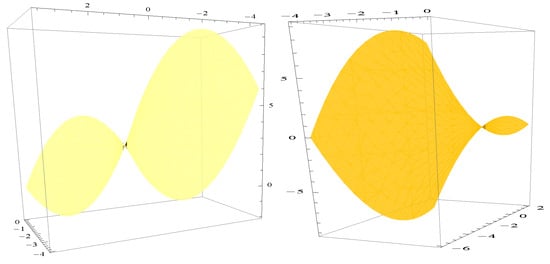
Figure 1 and Figure 2 are drawn for Equation (12); their functions are shown in their respective figures.
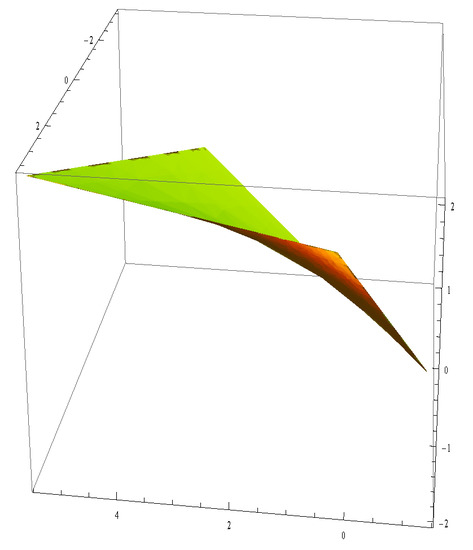
Figure 1.
and with , , .
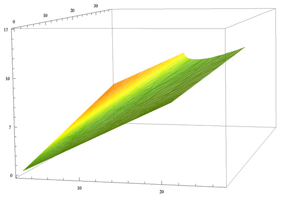
Figure 2.
and with , , .
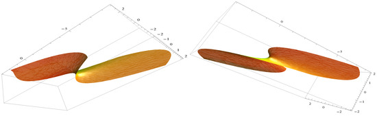
The Figure 3 with symmetry is drawn for (14) as an example where the constants and p are from Equation (12) and are from (13) [12,13,14].
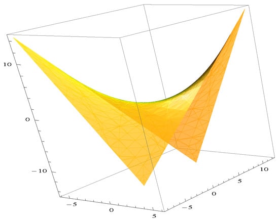
Figure 3.
and with , , .
Let us consider that the surface (14). Then, using the surface (14), the coefficients of the first and the second fundamental forms are given by
and
respectively. The isotropic Gaussian curvature and the mean curvatures , the isotropic Casorati curvature, the tangential curvature and the amalgamatic curvature of the surface (14) are given by
respectively. Let us assume that the surface (14) has a constant mean curvature. Then,
where If we use the separation of variables method, the mean curvature is a constant but 0, if and only if
where We can easily obtain
where
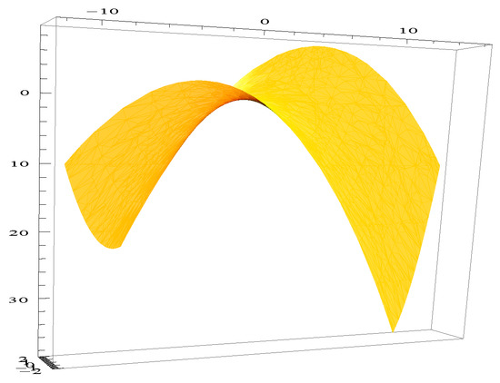
Figure 4.
and .
Suppose that the mean curvature of the constant negative curvature surface vanishes identically; then, from (22), we have
Here, u and v are independent variables, so each side of (25) is equal to a constant, called . Hence, the two equations are
With appropriate solutions to these differential equations, we have
where
Thus, we have the following results:
Theorem 1.
Theorem 2.
Theorem 3.
If the isotropic surface parametrized by (14) in has then
and if is a non-zero constant,
where where and .
Proof.
From (14), we have
where .
If from the solution of the Equation (29), we have
When we choose the constants at (28) as , we can obtain the figure with two different intervals as Figure 5.
Figure 5.
and .
Now, suppose that the second Gaussian curvature is a non-zero constant. The partial derivative of (29) with respect to u gives
Therefore, either, i.e., or
If , then we have
where If , then we have
By solving (33), we find
where , where and .
As we choose and , we can obtain the Figure 6, shown from two different angles. □
Figure 6.
.
Now, we consider the isotropic surface (14) in as satisfying as constant. From (21), we have
where Taking the partial derivative of (35) with respect to u gives
If then we have
where If then we have
where , where is positive.
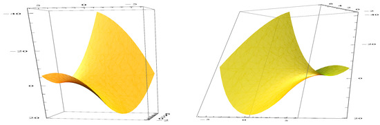
Figure 7.
and .
If the surface (14) has zero Casorati curvature (), then, by using a similar technique for the solution, we have
where
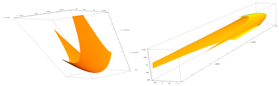
Figure 8.
and .
Let us assume that the isotropic surface (14) has a constant tangential curvature. Then from (22), we have
where By solving (22) we can find
where where

Figure 9.
and .
If the (14) has the constant amalgamatic curvature. Then, from (40), we obtain
where By solving (42), we find
where with .
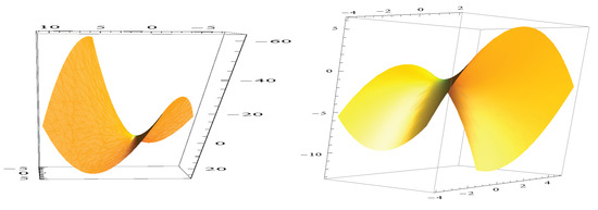
Figure 10.
and .
Author Contributions
Conceptualization, S.K.N. and İ.G.; methodology, S.K.N. and İ.G.; software, İ.G.; validation, S.K.N. and İ.G.; formal analysis, S.K.N. and İ.G.; investigation, S.K.N. and İ.G.; resources, S.K.N. and İ.G.; data curation, S.K.N. and İ.G.; writing—original draft preparation, S.K.N.; writing—review and editing, S.K.N. and İ.G.; visualization, S.K.N. and İ.G.; supervision, S.K.N.; project administration, S.K.N. and İ.G.; funding acquisition, S.K.N. and İ.G. All authors have read and agreed to the published version of the manuscript.
Funding
This research received no external funding.
Data Availability Statement
Not applicable.
Conflicts of Interest
The authors declare no conflict of interest.
References
- Bianchi, L. Lezioni di Geometria Differenziale; Ecole Bibliotheque: Pisa, Italy, 1902. [Google Scholar]
- Darboux, G. Lecons sur la Theorie Generate des Surfaces et les Applications Geometriques du Calcul Infinitesimal; Gauthier-Villars: Paris, France, 1887–1896; pp. 1–4. [Google Scholar]
- Pinkall, U. Designing Cylinders with Constant Negative Curvature. In Discrete Differential Geometry. Oberwolfach Seminars; Birkhäuser: Basel, Switzerland, 2008; Volume 38. [Google Scholar]
- Bobenko, A.; Pinkall, U.J. Discrete surfaces with constant negative Gaussian curvature and the Hirota equation. Differ. Geom. 1996, 43, 527–611. [Google Scholar] [CrossRef]
- Melko, M.; Sterling, I. Application of soliton theory to the construction of pseudospherical surfaces in R3. Ann. Glob. Anal. Geom. 1993, 11, 65–107. [Google Scholar] [CrossRef]
- Cieslinski, J.L. Pseudospherical surfaces on time scales: A geometric definition and the spectral approach. J. Phys. A Math. Theor. 2007, 40, 12525–12538. [Google Scholar] [CrossRef]
- Aldossary, M.T. Bäcklund’s Theorem for Spacelike Surfaces in Minkowski 3-Space. OSR J. Math. 2013, 5, 24–30. [Google Scholar]
- Tian, C. Bäcklund transformations for surfaces with K = −1 in 2,1. J. Geom. Phys. 1997, 22, 212–218. [Google Scholar] [CrossRef]
- Erdoğdu, M.; Özdemir, M. On Bäcklund Transformation Between Timelike Curves in Minkowski Space-Time. SDU J. Nat. Appl. Sci. 2018, 22, 1143–1150. [Google Scholar]
- Kim, Y.H.; Yoon, D.W. Classification of ruled surfaces in Minkowski 3-spaces. J. Geom. Phys. 2004, 49, 89–100. [Google Scholar] [CrossRef]
- López, R. Differential Geometry of Curves and Surfaces in Lorentz-Minkowski Space. Int. Electron. J. Geom. 2014, 7, 44–107. [Google Scholar] [CrossRef]
- Strubeckerr, K. Theorie der flachentreuen Abbildungen der Ebene, Contributions to Geometry. In Proceedings of the Geometry-Symposium, Siegen, Germany, 28 June–1 July 1978. [Google Scholar]
- Strubeckerr, K. Die Flächen konstanter Relativkrümmung K = rt − s2. Differentialgeometrie des isotropen Raumes II. Math. Z. 1942, 47, 743–777. [Google Scholar] [CrossRef]
- Strubecker, K. Die Flächen, deren Asymptotenlinien ein Quasi-Rückungsnetz bilden. Sitzungsberichte 1952, 12, 103–110. [Google Scholar]
- Decu, S.; Verstraelen, L. A note on the isotropical Geometry of production surfaces. Kragujev. J. Math. 2013, 37, 217–220. [Google Scholar]
- Brubaker, N.D.; Camero, J.; Rocha, O.R.; Suceava, B.D. A ladder of curvatures in the geometry of surfaces. Int. Electron. J. Geom. 2018, 11, 28–33. [Google Scholar]
- Casorati, F. Mesure de la courbure des surfaces suivant l’idée commune. Acta Math. 1890, 14, 95–110. [Google Scholar] [CrossRef]
- Koenderink, J.J. Shadows of Shapes; De Clootcrans Press: Utrecht, The Netherlands, 2012. [Google Scholar]
- Verstraelen, L. Geometry of submanifolds I. The first Casorati curvature indicatrices. Kragujev. J. Math. 2013, 37, 5–23. [Google Scholar]
- Conley, C.; Etnyre, R.; Gardener, B.; Odom, L.H.; Suceava, B.D. New Curvature Inequalities for Hypersurfaces in the Euclidean Ambient Space. Taiwan. J. Math. 2013, 17, 885–895. Available online: http://www.jstor.org/stable/taiwjmath.17.3.885 (accessed on 12 April 2023). [CrossRef]
- Weingarten, J. Uber eine Klasse aufeinander abwickelbarer Flachen. J. F’Ur Die Reine Angew. Math. 1861, 59, 382–393. [Google Scholar]
- Weingarten, J. Uber die Flachen, derer Normalen eine gegebene Flache beruhren. J. Fur Die Reine Angew. Math. 1863, 62, 61–63. [Google Scholar]
- Hartman, P.; Wintner, A. Umbilical points and W-surfaces. Am. J. Math. 1954, 76, 502–508. [Google Scholar] [CrossRef]
- Chern, S.S. On special W-surfaces. Proc. Am. Math. Soc. 1955, 6, 783–786. [Google Scholar] [CrossRef]
- Chen, B.Y. Pseudo-Riemannian Geometry, δ-Invariants and Applications; World Scientific: Singapore, 2011. [Google Scholar]
- Šipuš, Ž.M. Translation surfaces of constant curvatures in a simply isotropic space. Period Math. Hung. 2014, 68, 160–175. [Google Scholar] [CrossRef]
- Sangwine, S.J. Perspectives on Color Image Processing by Linear Vector Methods Using Projective Geometric Transformations. In Advances in Imaging and Electron Physics; Elsevier: Amsterdam, The Netherlands, 2013; Volume 175, pp. 283–307. [Google Scholar] [CrossRef]
- Onishchik, A.L.; Sulanke, R. Projective and Cayley-Klein Geometries; Springer: Berlin, Germany, 2006. [Google Scholar] [CrossRef]
- Pottmann, H.; Grohs, P.; Mitra, N.J. Laguerre minimal surfaces, isotropic geometry and linear elasticity. Adv. Comput. Math. 2009, 31, 391–419. [Google Scholar] [CrossRef]
- Pottmann, H.; Liu, Y. Discrete Surfaces in Isotropic Geometry. Mathematics of Surfaces XII; Springer: Berlin, Germany, 2007; pp. 341–363. [Google Scholar]
- Yoon, D.W.; Lee, J.W. Linear Weingarten Helicoidal Surfaces in Isotropic Space. Symmetry 2016, 8, 126. [Google Scholar] [CrossRef]
- Lone, M.S.; Karacan, M.K. Dual Translation Surfaces in the Three Dimensional Simply Isotropic Space. Tamkang J. Math. 2018, 49, 67–77. [Google Scholar] [CrossRef]
- Güler, E.; Vanli, A.T. On The Mean, Gauss, The Second Gaussian and The Second Mean Curvature of The Helicoidal Surfaces with Light-Like Axis in . Tsukuba J. Math. 2008, 32, 49–65. [Google Scholar] [CrossRef]
- Sauer, V.R. Infinitesimale Verbiegung der Flächen, deren Asymptotenlinien ein Quasi-Rückungsnetz bilden. Sitz. Ber. Math. Naturw. Kl. Bayr. Akad. Wiss. 1950, 1, 1–12. [Google Scholar]
Disclaimer/Publisher’s Note: The statements, opinions and data contained in all publications are solely those of the individual author(s) and contributor(s) and not of MDPI and/or the editor(s). MDPI and/or the editor(s) disclaim responsibility for any injury to people or property resulting from any ideas, methods, instructions or products referred to in the content. |
© 2023 by the authors. Licensee MDPI, Basel, Switzerland. This article is an open access article distributed under the terms and conditions of the Creative Commons Attribution (CC BY) license (https://creativecommons.org/licenses/by/4.0/).