Virtual Sensors for Nonlinear Discrete-Time Dynamic Systems

Abstract

The problem of virtual sensor design for nonlinear systems under the disturbance is investigated. Two different mathematical techniques are used to solve the problem: the algebra of functions and the logic-dynamic approach. The first one allows obtaining a general solution while the second one produces a solution for nonlinear systems by linear algebra methods. The virtual sensors are designed to be insensitive to the disturbance based on invariant functions. They estimate the prescribed function of the original system state vector. The practical example illustrates theoretical results.

1. Introduction

Modern technical systems are provided by different sensors which are used, in particular, to solve control and fault diagnosis problems. To simplify the solution, one can use the additional physical sensors but this cannot always be realized in practice and may result in extra expenses. Moreover, as usual, such sensors are unreliable. In this case, one can use virtual sensors. Additionally, virtual sensors can replace the faulty physical sensor. Note that the virtual sensors are similar to the reduced-order observers, which estimate some of the system’s state variables. Virtual sensors are constructed to estimate the arbitrary nonlinear function of the system’s state vector.

Different problems in the design and application of virtual sensors are studied [1,2,3,4,5,6,7,8,9,10,11,12,13,14]. The practical applications of such sensors have mainly been for an automotive engine [1], an industrial motor [14], walking robots [6] and aircraft [7], and for fault diagnosis in a bicomponent mixing machine [8]. For remotely deployed sensors, a new architectural paradigm is presented in [10]. The different theoretical and practical aspects of virtual sensor design are considered in [2,4,9,11].

The main contribution of this paper is that virtual sensors which are insensitive or have minimal sensitivity to external disturbances are designed to estimate the prescribed function of the system state vector. Unlike [4], where the procedure to design virtual sensors estimating the entire state was developed for linear systems free of any external disturbances, this present paper considers the systems with non-smooth nonlinearities such as backlash, dry friction, saturation, and hysteresis, estimating the prescribed function of the state vector. Clearly, the use of the virtual sensors of the reduced dimension allows one to diminish the computational complexity and implement more effective control. Such sensors are designed using two different mathematical techniques. The first is the algebra of functions, allowing one to obtain the general solution developed in [15] and used to solve the different problems of nonlinear dynamic systems described by non-smooth nonlinearities. The second is the logic-dynamic approach developed in [16] which produces a solution for nonlinear systems by linear algebra methods. Such sensors estimate the prescribed components of the system state vector and are of the minimal dimension.

Consider the system given by the nonlinear model

$$x(t+1)=f\left(x\right(t),u(t),\rho (t\left)\right),y\left(t\right)=h\left(x\right(t\left)\right).$$

(1)

Here, $x\in X\subseteq R^n$ is the state vector, $u\in U\subseteq R^m$ is the vector of control, $y\in R^l$ is the vectors of the output; $\rho \left(t\right)\in R^s$ is an unknown function of time and describes the disturbance; f and h are nonlinear functions, and the function f may be non-smooth.

The problem is to design a virtual sensor that is insensitive to the disturbance and estimates the variable $v\left(t\right)=\nu \left(x\left(t\right)\right)\in {\mathbb{R}}^p$ for the specified function $\nu$. The reduced-order model

$$\begin{array}{c}\hfill z(t+1)=f_{*}(z\left(t\right),u\left(t\right),y\left(t\right),v\left(t\right)),v\left(t\right)=h_v(z\left(t\right),y_0\left(t\right)),\end{array}$$

(2)

is used to design such a sensor. Here, $z\in R^k$ is the vector of the state, $f_{*}$ and $h_v$ are functions to be determined and the variable $y_0\left(t\right)$ will be explained below.

We consider two mathematical techniques to design the model (2): the general solution is based on the algebra of functions while the logic-dynamic approach produces a solution for nonlinear systems by methods of linear algebra.

2. General Solution

The general approach to the model (2) design is based on the algebra of functions developed in [15] and used to solve the different problems of system theory [15,17,18,19] and briefly described in Appendix A. The elements of this algebra are the functions determined on X. The algebra of the functions contains: the relation of the partial pre-order ≤, binary operations × and ⊕, binary relation $\Delta$, and operators $\mathbf{m}$ and $\mathbf{M}$.

One assumes that there exists the function $\psi$ such that $z\left(t\right)=\psi \left(x\right(t\left)\right).$ It follows from (2) that the considered problem is closed to the fault diagnosis problem described in terms of the algebra of functions in [15,17]. The differences are the variable $v\left(t\right)$ in the function $f_{*}$ and $y_0\left(t\right)$ in the function $h_v$. The similarity of these problems allows to conclude that the function $\psi$ satisfies the condition [15,17]

$$\psi \times h_{*}\le \mathbf{M}\left(\psi \right),$$

(3)

where $h_{*}\left(x\right)=(h\times \nu )\left(x\right)=\left(\begin{array}{c}\hfill h\left(x\right)\\ \hfill \nu \left(x\right)\end{array}\right)=\left(\begin{array}{c}\hfill y\\ \hfill v\end{array}\right).$

Note that the function $\psi$ is $(h_{*},f)$-invariant and is similar to that used in [20] to solve the different problems of control theory.

The case when the model is insensitive to the disturbance is the best solution. Such a model can be designed as follows. Let ${\gamma }^0$ be a minimal function (in the sense of the relation ≤) such that $\rho$ is not in ${\gamma }^0\left(f(x,u,\rho )\right)$. The sequence of functions ${\gamma }^0\le {\gamma }^1\le \dots$ is defined using the formula

$${\gamma }^{i+1}={\gamma }^i\oplus \mathbf{m}({\gamma }^i\times h_{*}),i=0,1,\dots$$

One proves that for some finite k the relation ${\gamma }^{k+1}={\gamma }^k$ is true [15,19]. Define $\psi :={\gamma }^k.$

Theorem 1

([15,19]). The function ψ is minimal, meeting the conditions (3) and ${\gamma }^0\le \psi$.

The relation ≤ and the operator $\mathbf{M}$ mean that the condition (3) implies the existence of the function $f_{*}$ satisfying the equality

$$f_{*}((\psi \times h_{*})\left(x\left(t\right)\right),u\left(t\right))=\psi \left(f(x\left(t\right),u\left(t\right),\rho \left(t\right))\right);$$

(4)

whilst, additionally, it follows from ${\gamma }^0\le \psi$ that the function $f_{*}$ does not contain the disturbance $\rho \left(t\right)$.

To avoid the influence of $\rho \left(t\right)$ on $v\left(t\right)$, the variable $y_0\left(t\right)$ in (2) should not also contain $\rho \left(t\right)$. This means that this variable should be such part of the vector $y\left(t\right)=h\left(x\right(t\left)\right)$ which is insensitive to the disturbance: $y_0\left(t\right)=({\gamma }^0\oplus h)\left(x\left(t\right)\right)$. Denote $h_0={\gamma }^0\oplus h$.

To design the dynamic part of the model (2), perform the transformation according to (4) of the right hand side of the relation

$$z(t+1)=\psi \left(x\right(t+1\left)\right)=\psi \left(f\right(x\left(t\right),u\left(t\right),\rho \left(t\right)\left)\right)$$

To design the static part in the form $v=h_v(z,y_0)$, write down it as follows:

$$\nu \left(x\right)=h_v(\psi \left(x\right),h_0\left(x\right)),$$

(5)

which is equivalent to the functional inequality

$$\psi \times h_0\le \nu .$$

(6)

If this condition is true for the function $\psi$, then based on (6) and the relation ≤, the function $h_v$ can be calculated. As a result, the model (2) was designed.

Recall that the function $\psi$ is minimal; this provides the best condition to satisfy (6) but produces the model of maximal dimensions. To simplify the model, one has to find the function ${\psi }_{*}$ satisfying the conditions

$$\psi \le {\psi }_{*},h_{*}\times {\psi }_{*}\le \mathbf{M}\left({\psi }_{*}\right).$$

(7)

Since ${\gamma }^0\le \psi$, then ${\gamma }^0\le {\psi }_{*}$, and ${\psi }_{*}$ can be used instead of $\psi$.

If the condition (6) is not satisfied, one cannot design the model insensitive to the disturbance. In this case, to design the model weakly sensitive to the disturbance, one has to supplement the function $\psi$ by the maximal (containing the minimal number of independent components) function ${\psi }^{\prime }$ satisfying the condition

$$\psi \times {\psi }^{\prime }\times h_0\le \nu .$$

(8)

Since the function ${\psi }^{\prime }$ is ambiguously defined, it should be chosen so that the contribution of the disturbance $\rho \left(t\right)$ in the function ${\psi }^{\prime }\left(f(x,u,\rho )\right)$ is minimal.

Remark 1.

If the system is linear and is described by matrix equations, one can formulate the precise definition of the disturbance $\rho \left(t\right)$ contribution in the model and then solve the problem to minimize this contribution [21]. Generally, one may call this weak sensitivity.

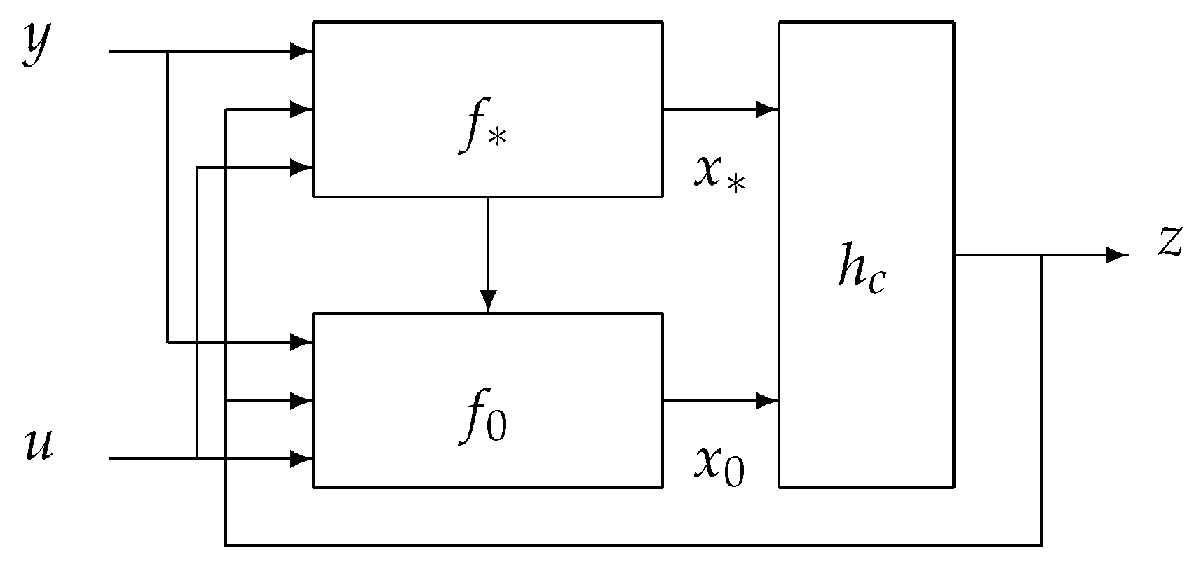
As a result, the total model is a composition of system (2) being insensitive to the disturbance and new system with the state vector $z_0={\psi }_0\left(x\right)$ (Figure 1), where function ${\psi }_0$ satisfies conditions

$${\psi }_0\le {\psi }^{\prime },(\psi \times h_{*})\times {\psi }_0\le \mathbf{M}\left({\psi }_0\right).$$

(9)

The first condition means that the function ${\psi }_0$ contains information no less than ${\psi }^{\prime }$ and can be used in (8) instead of ${\psi }^{\prime }$. The second condition is similar to the inequality (3) and describes the dynamic of the second system in Figure 1.

Figure 1. The total model.

The algorithm below (Algorithm 1) is used to compute the function ${\phi }_0$ satisfying the conditions in (9) [15,19].

Algorithm 1: Computation of the function ${\phi }_0$

1. Set $i:=1$, ${\beta }^1:={\phi }^{\prime }$.

2. Compute the function ${\gamma }^i=\mathbf{M}\left({\beta }^i\right)$.

3. If ${\gamma }^i$ can be expressed via $\phi \times h_{*}\times {\beta }^1\times \dots \times {\beta }^i$, go to Step 5.

4. Find the function ${\beta }^{i+1}$ with a minimal number of components satisfying the inequality

$$(\phi \times h_{*})\times {\beta }^1\times \dots \times {\beta }^i\times {\beta }^{i+1}\le {\gamma }^i,$$ (10)

set $i:=i+1$ and go to Step 2.

5. Set ${\phi }_0:={\beta }^1\times \dots \times {\beta }^i$.

The algorithm does not guarantee that ${\psi }_0$ is unique, since different functions ${\beta }^{i+1}$ (incomparable in the sense of the relation ≤) satisfying the conditions (10) can be chosen at Step 4. More information about the algorithm can be found in [15,19].

The final model is given by

$$\begin{array}{ccc}\hfill z(t+1)& =& f_{*}(z\left(t\right),u\left(t\right),y\left(t\right),v\left(t\right)),\hfill \\ \hfill z_0(t+1)& =& f_0(z_0\left(t\right),z\left(t\right),u\left(t\right),y\left(t\right),v\left(t\right)),\hfill \\ \hfill v\left(t\right)& =& h_c(z_0\left(t\right),z\left(t\right),y_0\left(t\right)),\hfill \end{array}$$

(11)

where the functions $h_c$ and $f_0$ are defined based on relations (8) (after replacing the function ${\psi }^{\prime }$ by ${\psi }_0$) and (9), respectively.

The stability of the model (2) or (11) can be achieved by known methods [22]; some of them are considered in Section 4.

3. Logic-Dynamic-Based Solution

3.1. Insensitivity to the Disturbance

When the function $\psi$ is assumed to be nonlinear, the theorem gives a general solution to the problem and demands a complex mathematical technique—the algebra of functions. If one limits a class of functions $\psi$ by linear functions, the solution can be obtained by the logic-dynamic approach [16] which is based on the linear algebra. To use this approach, system (1) should be presented in the form

$$\begin{array}{ccc}\hfill x(t+1)& =& Ax\left(t\right)+Bu\left(t\right)+G\Phi \left(x\right(t),u(t\left)\right)+D\rho \left(t\right),\hfill \\ \hfill y\left(t\right)& =& Cx\left(t\right),\hfill \end{array}$$

(12)

where A, B, and C are matrices, the matrix D describes the disturbance, the contribution of nonlinear terms G is presented in the form

$$\Phi (x\left(t\right),u\left(t\right))=\left(\begin{array}{c}{\varphi }_1(F_{1}x\left(t\right),u\left(t\right))\\ \dots \\ {\varphi }_q(F_{q}x\left(t\right),u\left(t\right))\end{array}\right);$$

${\varphi }_1$, …, ${\varphi }_q$ are nonlinearities, and $F_1$, …, $F_q$ are the matrices. One assumes that $v\left(t\right)=Vx\left(t\right)$ for the prescribed matrix V. System (12) can be obtained from (1) [16].

Note that the nonlinear smooth systems can be studied by geometric approaches [20,23]; in our case, where the systems with non-smooth nonlinearities are considered, these approaches cannot be applied.

As is already known [16], there are three steps in the logic-dynamic approach: at the first step, one removes the nonlinear term from (12); then, the linear model is designed with additional restriction; finally, one transforms the nonlinear term and adds it in the linear model. The linear model at the second step is given by

$$\begin{array}{ccc}\hfill z(t+1)& =& A_{*}{x}_{*}\left(t\right)+J_{*}{y}_{*}\left(t\right)+B_{*}u\left(t\right),\hfill \\ \hfill v\left(t\right)& =& C_v{x}_{*}\left(t\right)+Q{y}_0\left(t\right),\hfill \end{array}$$

(13)

where $y_{*}\left(t\right)=C_{*}x\left(t\right)=\left(\begin{array}{c}y\left(t\right)\\ z\left(t\right),\end{array}\right)$, $C_{*}=\left(\begin{array}{c}C\\ V\end{array}\right).$

As above, the variable $y_0\left(t\right)$ in (13) must be insensitive to the disturbance $\rho \left(t\right)$. To obtain such a variable, introduce the matrix $D_0$ of the maximal rank such that $D_{0}D=0$; note that $D_0$ corresponds to the function ${\gamma }^0$. Clearly, $x^{\prime }=D_{0}x$ is insensitive to $\rho \left(t\right)$ and $y_0=N_1{x}^{\prime }=N_1{D}_{0}x$ for some matrix $N_1$. Additionally, since $y_0$ is a part of the vector y, then $y_0=N_{2}Cx$ for some matrix $N_2$. Both equalities result in the equation $N_1{D}_0=N_{2}C$. The matrices $N_1$ and $N_2$ of maximal rank can be found from the equation

$$(N_1-N_2)\left(\begin{array}{c}{D}_0\\ C\end{array}\right)=0.$$

(14)

Finally, one set $y_0\left(t\right)=N_{2}Cx\left(t\right)=N_{2}y\left(t\right).$

Recall that $z\left(t\right)=\psi \left(x\right(t\left)\right)$ for some function $\psi$ in Section 2; here, this function is assumed to be linear and $z\left(t\right)=\Psi x\left(t\right)$ for some matrix $\Psi$. It is known that this function satisfies the condition [16]

$$\Psi A=A_{*}\Psi +J_{*}{C}_{*},B_{*}=\Psi B.$$

(15)

Besides one assumes that matrix $A_{*}$ is in canonical form. In [24], two different forms are considered: identification and Jordan ones; it was shown that, for the continuous-time systems, the Jordan form is preferable from the point of view of stability. The identification of the canonical form with the matrix

$$A_{*}=\left(\begin{array}{ccccc}0& 1& 0& \dots & 0\\ 0& 0& 1& \dots & 0\\ \dots & \dots & \dots & \dots \\ 0& 0& 0& \dots & 0\end{array}\right),$$

(16)

has zero eigenvalues, ensuring that the stability is therefore preferable for the discrete-time systems.

The matrices describing system (12) and model (13) meet the following equations based on (15) and (16) [16,24]:

$${\Psi }_{i}A={\Psi }_{i+1}+J_{*i}{C}_{*},i=1,\dots ,k-1,{\Psi }_{k}A=J_{*k}{C}_{*}.$$

Here, ${\Psi }_i$ and $J_{*i}$ are i-th rows of matrices $\Psi$ and $J_{*}$, respectively, $i=1,\dots ,k.$ Since system (12) contains the nonlinearity $\Phi (x,u)$ and model (13) contains the variable $v\left(t\right)$, the matrix $\Psi$ should satisfy additional restrictions. The first of them has the form [16]

$$F^{\prime }=F_{*}\left(\begin{array}{c}\Psi \\ C_{*}\end{array}\right)$$

(17)

for some matrix $F_{*}$. Here,

$$F^{\prime }=\left(\begin{array}{c}{F}_{j_1}\\ \dots \\ F_{j_d}\end{array}\right),$$

the numbers $j_1,j_2,\dots ,j_d$ denote nonzero columns in $\Psi C$. The equality (17) is solvable if

$$\mathrm{rank}\left(\begin{array}{c}\Psi \\ C_{*}\end{array}\right)=\mathrm{rank}\left(\begin{array}{c}\Psi \\ C_{*}\\ F^{\prime }\end{array}\right).$$

(18)

The second restriction arises from the demand $v\left(t\right)=Vx\left(t\right)$ and (13), which imply

$$V=C_z\Psi +Q{C}_0=\left(C_{z}Q\right)\left(\begin{array}{c}\Psi \\ C_0\end{array}\right).$$

(19)

This equation is solvable if

$$\mathrm{rank}\left(\begin{array}{c}\Psi \\ C_0\end{array}\right)=\mathrm{rank}\left(\begin{array}{c}\Psi \\ C_0\\ V\end{array}\right).$$

(20)

The inequalities (18) and (20) are the desired additional restrictions.

The condition $\Psi D=0$ guarantees that the model is insensitive to the disturbance; this demand can be presented in the form [21]

$$\begin{array}{cccc}({\Psi }_1& -J_{*1}& \dots & -J_{*k})\end{array}\left(W^{\left(k\right)}{D}^{\left(k\right)}\right)=0,$$

(21)

where

$$\begin{array}{ccc}\hfill W^{\left(k\right)}& =& \left(\begin{array}{c}{A}^k\\ C_{*}{A}^{k-1}\\ \dots \\ C_{*}\end{array}\right),\hfill \\ \hfill D^{\left(k\right)}& =& \left(\begin{array}{ccccc}D& AD& A^{2}D& \dots & A^{k-1}D\\ 0& C_{*}D& C_{*}AD& \dots & C_{*}{A}^{k-2}D\\ \dots & \dots & \dots & \dots & \dots \\ 0& 0& 0& \dots & 0\end{array}\right).\hfill \end{array}$$

This equation is solvable if

$$\mathrm{rank}\left(W^{\left(k\right)}{D}^{\left(k\right)}\right)<n+(l+p)k.$$

(22)

If it is true, the matrix $\begin{array}{cccc}({\Psi }_1& -J_{*1}& \dots & -J_{*k})\end{array}$ exists and satisfies the condition (21). Then, the matrix $\Psi$ is found and the conditions (18) and (20) are checked; if they are fulfilled, the matrices $F_{*}$, $C_z$, Q, and $B_{*}$ can be found from (17), (19) and (15), respectively. If (18) or (20) are not fulfilled, another solution of (21) should be found. In what follows, we assume that (18) and (20) are satisfied.

The transformed nonlinear term is given by

$$G_{*}\Phi (z\left(t\right),y_{*}\left(t\right),u\left(t\right))=G_{*}\left(\begin{array}{c}{\varphi }_{j_1}(F_{*j_1}w\left(t\right),u\left(t\right))\\ \dots \\ {\varphi }_{j_d}(F_{*j_d}w\left(t\right),u\left(t\right))\end{array}\right),$$

(23)

where $w=\left(\begin{array}{c}z\\ y_{*}\end{array}\right).$ One can find the matrices $F_{*j_1}$, …, $F_{*j_d}$ from the equation $F_j^{\prime }=F_{*j}\left(\begin{array}{c}\Psi \\ C_{*}\end{array}\right),$$j=j_1,\dots ,j_d,$ corresponding to (17). The term (23) is added to the model (13), and a nonlinear model which is insensitive to the disturbance was designed.

3.2. Sensitive to the Disturbance Solution

If (21) has no solutions or (18) or (20) are not satisfied for all $k<n$, the nonlinear model insensitive to the disturbance cannot be designed. Here, one has to use the robust method based on the singular value decomposition described in [21].

Consider another approach to obtain a robust solution based on the composition Figure 1. Assume that the matrix $\Psi$ is found from (21) and the condition (18) is satisfied while (20) is not. Find all the rows of matrix V for which the condition (20) is satisfied, denote them by $V^{\prime }$, and design the model (the first subsystem in Figure 1) estimating the vector $v^{\prime }\left(t\right)=V^{\prime }x\left(t\right)$ insensitive to the disturbance. The rest of the rows, denoted by $V_0$, are used to design the model (the second subsystem)

$$\begin{array}{ccc}\hfill z_0(t+1)& =& A_{*}{z}_0\left(t\right)+J_{0}v\left(t\right)+B_{0}u\left(t\right),\hfill \\ \hfill v_0\left(t\right)& =& C_0{z}_0\left(t\right)+Q_{0}y\left(t\right),\hfill \end{array}$$

(24)

estimating the variable $v_0\left(t\right)=V_{0}x\left(t\right).$ The first row of the matrix ${\Psi }_0$ such that $z_0\left(t\right)={\Psi }_{0}x\left(t\right)$ is found from the equation

$$\begin{array}{cccc}({\Psi }_{01}& -J_{01}& \dots & -J_{0k})\end{array}{W}_0^{\left(k\right)}=0$$

(25)

for minimal k, where

$$W_0^{\left(k\right)}=\left(\begin{array}{c}{A}^k\\ C_c{A}^{k-1}\\ \dots \\ C_c\end{array}\right),C_c=\left(\begin{array}{c}\Psi \\ C_{*}\end{array}\right)=\left(\begin{array}{c}\Psi \\ C\\ V\end{array}\right).$$

Then, the matrix ${\Psi }_0$ is found and the conditions (18) or (20) are checked after replacing the matrices $\Psi$, $C_{*}$, and V by ${\Psi }_0$, $C_c$, and $V_0$, respectively. If these conditions are satisfied, compute the matrices $H_0$, $Q_0$, $G_0={\Psi }_{0}G$, and $B_0={\Psi }_{0}B$ and the linear model (24) is designed. The nonlinear term has the form

$$G_0\left(\begin{array}{c}{\varphi }_{i_1}(F_{0i_1}{w}_0\left(t\right),u\left(t\right))\\ \dots \\ {\varphi }_{i_g}(F_{0i_g}{w}_0\left(t\right),u\left(t\right))\end{array}\right),$$

where $w_0=\left(\begin{array}{c}{z}_0\\ v\end{array}\right),$ $i_1,i_2,\dots ,i_g$ are numbers of nonzero columns in $G_0={\Psi }_{0}G.$ The rows $F_{0i_1}$, …, $F_{0i_g}$ are found from the equation $F_i^{″}=F_{0i}\left(\begin{array}{c}{\Psi }_0\\ C_c\end{array}\right),$$i=i_1,\dots ,i_g,$ where

$$F^{″}=\left(\begin{array}{c}{F}_{i_1}\\ \dots \\ F_{i_g}\end{array}\right).$$

If (18) or (20) is not satisfied, one has to find another solution of (25) with a former or incremented k. The total model is a composition of the models (13) and (24) supplemented by nonlinear terms.

To the contrary, if the condition (20) is satisfied while (18) is not, the model can be analogously designed by analyzing the matrix $F^{\prime }$.

4. Stability of the Model

If $G_{*}=0$, the model is linear and its stability is ensured by the canonical form of the matrix $A_{*}$, otherwise, an additional analysis is required. Consider this in detail; define the error $e\left(t\right)=\Psi x\left(t\right)-z\left(t\right).$

Assume that the error $e\left(t\right)$ is small and the function $\Phi (z,y_{*},u)$ is differentiable with respect to z. Initially consider the case when $q=1$ and $\Phi (x,u)=\varphi (Ax,u)$. Since $F=F_{*}\left(\begin{array}{c}\Psi \\ C_{*}\end{array}\right)$ and $e=\Psi x-z$, then

$$Fx=F_{*}\left(\begin{array}{c}\Psi \\ C_{*}\end{array}\right)x=F_{*}^1\Psi x+F_{*}^2{F}_{*}x=F_{*}^1(z+e)+F_{*}^2{y}_{*},$$

where $F_{*}=\left(F_{*}^1{F}_{*}^2\right)$. The function $\Delta \Phi \left(t\right)$ can be transformed as

$$\begin{array}{ccc}\hfill \Delta \Phi \left(t\right)& =& G_{*}(\varphi (Fx\left(t\right),u\left(t\right))-\varphi (F_{*}^{1}z\left(t\right)+F_{*}^2{y}_{*}\left(t\right),u\left(t\right)))\hfill \\ & =& G_{*}(\varphi (F_{*}^1(z\left(t\right)+e\left(t\right))+F_{*}^2{y}_{*}\left(t\right),u\left(t\right))\hfill \\ & & -\varphi (F_{*}^{1}z\left(t\right)+F_{*}^2{y}_{*}\left(t\right),u\left(t\right)))\hfill \\ & \approx & G_{*}\frac{\partial \varphi (z,y_{*},u)}{\partial z}{F}_{*}^{1}e\left(t\right).\hfill \end{array}$$

As a result, the final relation for $e\left(t\right)$ is given by

$$e(t+1)=\left(A_{*}+G_{*}\frac{\partial \varphi (z,y_{*},u)}{\partial z}{F}_{*}^1\right)e\left(t\right)=A_e(z,y_{*},u)e\left(t\right).$$

If the eigenvalues of the matrix $A_e(z,y_{*},u)$ are in the unit circle, the model is stable. Otherwise, one has to use a feedback with the residual $r\left(t\right)=R_{r}y\left(t\right)-y_r\left(t\right),$ where the matrix $R_r$ satisfies the condition $R_{r}C=C_r\Psi$ for some matrix $C_r$ and $y_r\left(t\right)=C_r{x}_{*}\left(t\right)$ [21]. These matrices can be found from the equation

$$(C_r-R_r)\left(\begin{array}{c}\Psi \\ C\end{array}\right)=0.$$

The nonlinear model with the feedback $Kr\left(t\right)$ is given by

$$\begin{array}{c}\hfill z(t+1)=A_{*}z\left(t\right)+J_{*}{y}_{*}\left(t\right)+B_{*}u\left(t\right)+G_{*}\Phi (z\left(t\right),y_{*}\left(t\right),u\left(t\right))+Kr\left(t\right).\end{array}$$

The equation for the error becomes

$$e(t+1)=\left(A_{*}-K{C}_r+G_{*}\frac{\partial \varphi (z,y_{*},u)}{\partial z}{F}_{*}^1\right)e\left(t\right)=A_r(z,y_{*},u)e\left(t\right).$$

This equation implies that the feedback matrix K depends on $z,y_{*},u$. This matrix can be constructed as follows: find the characteristic polynomial of the matrix $A_r(z,y_{*},u)$

$$det(A_r(z,y_{*},u)-\lambda I_k)={\lambda }^k+a_1(K,z,y_{*},u){\lambda }^{k-1}+\dots +a_k(K,z,y_{*},u),$$

specify the eigenvalues ${\lambda }_1,\dots ,{\lambda }_k$, obtain the nonlinear equations

$$\begin{array}{ccc}\hfill a_1(K,z,y_{*},u)& =& -({\lambda }_1+{\lambda }_2+\dots +{\lambda }_k),\hfill \\ \hfill a_1(K,z,y_{*},u)& =& {\lambda }_1{\lambda }_2+{\lambda }_1{\lambda }_3+\dots +{\lambda }_{k-1}{\lambda }_k,\hfill \\ & \dots & \\ \hfill a_k(K,z,y_{*},u)& =& {(-1)}^k{\lambda }_1{\lambda }_2\dots {\lambda }_k,\hfill \end{array}$$

and find elements of the matrix K.

If the model has several nonlinearities, one obtains

$$A_r(z,y_{*},u)=A_{*}-K{C}_r+G_{*}\left(\begin{array}{c}(\partial {\varphi }_{j_i}(z,y_{*},u)/\partial z)F_{*j_1}^1\\ \dots \\ (\partial {\varphi }_{j_d}(z,y_{*},u)/\partial z)F_{*j_d}^1\end{array}\right).$$

In practice, the suggested approach can be used for a model of no more than 3–4 dimensions since it results in complex impressions when the determinant $det(A_r(z,y_{*},u)-\lambda I_k)$ is calculated.

5. Practical Example

Consider the control system

$$\begin{array}{ccc}\hfill x_1(t+1)& =& a_4{u}_1\left(t\right)-a_1\sqrt{x_1\left(t\right)-x_2\left(t\right)}+x_1\left(t\right)+\rho \left(t\right),\hfill \\ \hfill x_2(t+1)& =& a_5{u}_2\left(t\right)+a_1\sqrt{x_1\left(t\right)-x_2\left(t\right)}-a_2\sqrt{x_2\left(t\right)-x_3\left(t\right)}+x_2\left(t\right),\hfill \\ \hfill x_3(t+1)& =& a_2\sqrt{x_2\left(t\right)-x_3\left(t\right)}-a_3\sqrt{x_3\left(t\right)}+x_3\left(t\right),\hfill \\ \hfill y\left(t\right)& =& x_2\left(t\right).\hfill \end{array}$$

(26)

Equation (26) constitutes a sampled-data model of the well-known three-tank system. The system consists of three consecutively united tanks. The liquid flows into the first and second tanks and follows from the third one through the pipe. The levels of liquid in the tanks are $x_1$, $x_2$, and $x_3$, respectively, and $a_1,\dots ,a_5$ are coefficients. It is assumed that $x_1\ge x_2\ge x_3$.

Design the virtual sensor estimation for the variables $x_1$ and $x_3$, that is $\nu =x_1\times x_3$. Compute the functions $h_{*}=(h\times \nu )=x_2\times x_1\times x_3=\mathbf{0}$, ${\gamma }^0=x_2\times x_3,$ and $h_0={\gamma }^0\oplus h=x_2$. Since ${\gamma }^0\times h_{*}=\mathbf{0}$, then $\mathbf{m}({\gamma }^0\times h_{*})=\mathbf{0}$, and so $\psi ={\gamma }^1={\gamma }^0=x_2\times x_3.$ Since $\psi \times h_0=(x_2\times x_3)\times x_2=x_2\times x_3,$ the condition (6) is not satisfied. The natural choice for ${\psi }^{\prime }$ in (8) is ${\psi }^{\prime }\left(x\right)=x_1.$ To compute ${\phi }_0$, one uses Algorithm 1 and obtains ${\psi }_0\left(x\right)=x_1.$ As a result, the second subsystem in Figure 1 with $z_1={\psi }_0\left(x\right)=x_1$ is given by

$$z_1(t+1)=a_4{u}_1\left(t\right)-a_1\sqrt{z_1\left(t\right)-y\left(t\right)}+z_1\left(t\right).$$

(27)

Since $\psi \left(x\right)=x_2\times x_3,$ the first subsystem in Figure 1 is two-dimensional. To reduce this subsystem, one may choose ${\psi }_{*}\left(x\right)=x_3$ which satisfies the condition (7). As a result, the first subsystem in Figure 1 with $z_2={\psi }_{*}\left(x\right)=x_3$ is given by

$$z_2(t+1)=a_2\sqrt{y\left(t\right)-z_2\left(t\right)}-a_3\sqrt{z_2\left(t\right)}+z_2\left(t\right).$$

(28)

The estimates of the variables $x_1$ and $x_3$ are as follows:

$${\widehat{x}}_1\left(t\right)=z_1\left(t\right),{\widehat{x}}_3\left(t\right)=z_2\left(t\right).$$

One can check that the model is stable, and therefore, the virtual sensor was designed.

Consider the logic-dynamic way to solve the problem. Clearly, $A=0$ in the model (12). To overcome this difficulty, transform Equation (26) by entering the formal addends $-a_1(x_1-x_2)+a_1(x_1-x_2),$$(a_1(x_1-x_2)-a_2(x_2-x_3))-(a_1(x_1-x_2)-a_2(x_2-x_3))$ and $a_2(x_2-x_3)-a_3{x}_3-a_2(x_2-x_3)+a_3{x}_3$ in the first, second, and third equations, respectively. The term $-a_1(x_1-x_2)$ refers to the linear part while $a_1(x_1-x_2)$ refers to the nonlinear part; the rest of the formal addends are considered analogously.

As a result, the system is described by matrices and nonlinearities as follows:

$$\begin{gathered} A=\left(\begin{array}{ccc}1-a_1& a_1& 0\\ -a_1& 1-a_1-a_2& a_2\\ 0& a_2& 1-a_2-a_3\end{array}\right),B=\left(\begin{array}{cc}1& 0\\ 0& 1\\ 0& 0\end{array}\right),C=\left(\begin{array}{ccc}0& 1& 0\end{array}\right), \\ D=\left(\begin{array}{c}1\\ 0\\ 0\end{array}\right),G=\left(\begin{array}{ccc}{a}_1& 0& 0\\ -a_1& a_2& 0\\ 0& -a_2& a_3\end{array}\right),\Phi \left(x\right)=\left(\begin{array}{c}-\sqrt{F_{1}x}+F_{1}x\\ -\sqrt{F_{2}x}+F_{2}x\\ -\sqrt{F_{3}x}+F_{3}x\end{array}\right), \\ {F}_1=(1-10),F_2=(01-1),F_3=\left(001\right). \end{gathered}$$

Since the variables $x_1$ and $x_3$ are estimated, then

$$V=\left(\begin{array}{ccc}1& 0& 0\\ 0& 0& 1\end{array}\right),C_{*}=\left(\begin{array}{ccc}0& 1& 0\\ 1& 0& 0\\ 0& 0& 1\end{array}\right),D_0=\left(\begin{array}{ccc}0& 1& 0\\ 0& 0& 1\end{array}\right).$$

The matrix $N_2$ is found from (14):

$$(N_1-N_2)\left(\begin{array}{ccc}0& 1& 0\\ 0& 0& 1\\ 0& 1& 0\end{array}\right)=0;$$

$N_2=1$ and $C_0=C=\left(010\right)$. Equation (21) has a solution with $k=1$:

$$\Psi =\left(001\right),J_{*}=(a_{2}01-a_2-a_3).$$

One may check that the condition (18) is satisfied, whilst (20) is not. Clearly, $V^{\prime }=\left(001\right)$ and $V_0=\left(100\right).$

The solution for $V^{\prime }$ with $\Psi =\left(001\right)$ produces the matrices $B_{*}=\left(00\right)$, $G_{*}=(0-a_2{a}_3),$ and $F^{\prime }=\left(\begin{array}{ccc}0& 1& -1\\ 0& 0& 1\end{array}\right)$. The solution of (17) is

$$F_{*}=\left(\begin{array}{cccc}-1& 1& 0& 0\\ 1& 0& 0& 0\end{array}\right).$$

The linear model corresponding to $V^{\prime }$ with $z_2=v^{\prime }=V^{\prime }x$ is given by

$$z_2(t+1)=a_{2}y\left(t\right)+(1-a_2-a_3)z_2\left(t\right);$$

and the nonlinear term is of the form

$$G_{*}\Phi (x,u)=a_2\sqrt{y\left(t\right)-z_2\left(t\right)}-a_2(y\left(t\right)-z_2\left(t\right))-a_3\sqrt{z_2\left(t\right)}+a_3{z}_2\left(t\right).$$

As a result, after inserting this term into the linear model and transforming it, one obtains the nonlinear model (28).

For $V_0$, Equation (25) has a solution with $k=1$:

$${\Psi }_0=\left(100\right),J_0=\left(100\right),$$

which produces $B_{*}=\left(a_{4}0\right)$, $G_0=\left(a_{1}00\right),$ $F^{\prime }=\left(\begin{array}{ccc}1& -1& 0\end{array}\right)$ and $F_0=(1-100).$ The linear model corresponding to $V_0$ with $z_1=v_0=V_{0}x$ being given by

$$z_1(t+1)=a_4{u}_1\left(t\right)+a_{1}y\left(t\right)+(1-a_1)z_1\left(t\right);$$

the nonlinear term is of the form

$$G_0\Phi (x,u)=-a_1\sqrt{z_1\left(t\right)-y\left(t\right)}+a_1(z_1\left(t\right)-y\left(t\right)).$$

After inserting this term into the linear model and transforming it, one obtains the nonlinear model (27).

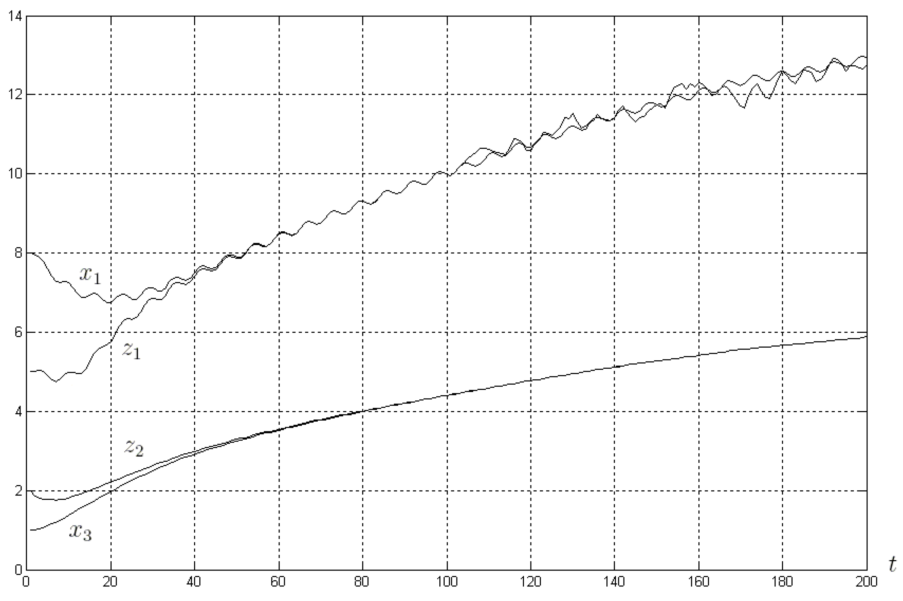
For simulation, consider system (26) and the sensor with the control $u_1\left(t\right)=u_2\left(t\right)=1+sin\left(t\right)$, $a_1=\dots =a_4=0.1$, $a_5=0.2$, $\rho \left(t\right)$ is a random process evenly distributed on $[-0.15,0.15]$ appearing at $t=100$. Simulation results are shown in Figure 2, where the variables $x_1\left(t\right)$, $x_3\left(t\right)$ and their estimates $z_1\left(t\right)$, $z_2\left(t\right)$ are presented for the initial conditions $x_1\left(0\right)=8,x_2\left(0\right)=2,x_3\left(0\right)=1,x_{*1}\left(0\right)=5,x_{*2}\left(0\right)=2$. Clearly, whilst the first sensor is sensitive to the disturbance, the second one is not.

Figure 2. Behavior of variables $x_1$ and $x_3$ and virtual sensors $z_1$ and $z_2$.

6. Discussion

The problem of virtual sensor design estimating the prescribed function of the state vector of the original system for nonlinear systems described by discrete-time models under the disturbance was studied. Two different mathematical techniques are used to solve the problem: the algebra of functions allows one to obtain a general solution and the logic-dynamic approach produces a solution for nonlinear systems by methods of linear algebra. The relations allowing one to design virtual sensor that is insensitive or that has minimal sensitivity to the disturbance were obtained. The theoretical results were illustrated by a practical example. A future research direction is the virtual sensor design for hybrid nonlinear dynamic systems.

The virtual sensors can be used in addition to the physical sensors in different practical systems or for replacing the faulty physical sensor. In particular, in [25,26], where the fault detection and estimation problems are considered, the additional virtual sensors allow simplifying the obtained solutions. Additionally, the algebra of the functions and the logic-dynamic approach enables one to extend a class of systems studied in [25,26] to systems with non-smooth nonlinearities.

References

- Ahmed, Q.; Bhatti, A.; Iqbal, M. Virtual sensors for automotive engine sensors fault diagnosis in second-order sliding modes. IEEE Sens. J. 2011, 11, 1832–1840. [Google Scholar] [CrossRef]
- Albertos, P.; Goodwin, G. Virtual sevrors for control application. Annu. Rev. Control. 2002, 26, 101–112. [Google Scholar] [CrossRef]
- Berkhoff, A.; Hekman, T. Active noise control using finite element-based virtual sensors. In Proceedings of the IEEE International Conference on Acoustics, Speech and Signal Processing (ICASSP), Brighton, UK, 12–17 May 2019. [Google Scholar]
- Blanke, M.; Kinnaert, M.; Lunze, J.; Staroswiecki, M. Diagnosis and Fault Tolerant Control; Springer: Berlin, Germany, 2016. [Google Scholar]
- Galavizh, A.; Hassanabadi, A. Designing fuzzy fault tolerant controller for a DC microgrid based on virtual sensor. In Proceedings of the 7th International Conference on Control, Instrumentation and Automation (ICCIA), Tabriz, Iran, 23–24 February 2021. [Google Scholar]
- Hashlamon, I.; Erbatur, K. Joint sensor fault detection and recovery based on virtual sensor for walking legged robots. In Proceedings of the IEEE 23rd International Symposium on Industrial Electronics, ISIE 2014, Istanbul, Turkey, 1–4 June 2014; pp. 1204–1210. [Google Scholar]
- Heredia, G.; Ollero, A. Virtual sensor for failure detection, identification and recovery in the transition phase of a morphing aircraft. Sensors 2010, 10, 2188–2201. [Google Scholar] [CrossRef]
- Jove, E.; Casteleiro-Roca, J.; Quntian, H.; Mendez-Perez, J.; Calvo-Rolle, J. Virtual sensor for fault detection, isolation and data recovery for bicomponent mixing machine monitoring. Informatica 2019, 30, 671–687. [Google Scholar] [CrossRef]
- Luzar, M.; Witczak, M. Fault-tolerant control and diagnosis for LPV system with H-infinity virtual sensor. In Proceedings of the 3rd Conference Control and Fault-Tolerant Systems, Barcelona, Spain, 7–9 September 2016; pp. 825–830. [Google Scholar]
- Trevathan, J.; Read, W.; Sattar, A.; Schmidtke, S.; Sharp, T. The virtual sensor concept. In Proceedings of the 2020 IEEE Sensors, Rotterdam, The Netherlands, 25–28 October 2020. [Google Scholar]
- Wang, Y.; Rotondo, D.; Puig, V.; Cembrano, G. Fault-tolerant control based on virtual actuator and sensor for discrete-time descriptor systems. IEEE Trans. Circuits Syst. 2020, 67, 5316–5325. [Google Scholar] [CrossRef]
- Witczak, M. Fault Diagnosis and Fault Tolerant Control Strategies for Nonlinear Systems; Springer: Berlin, Germany, 2014. [Google Scholar]
- Roy, C.; Roy, A.; Misra, S. DIVISOR: Dynamic virtual sensor formation for overlapping region in IoT-based sensor-cloud. In Proceedings of the 2018 IEEE Wireless Communications and Networking Conference, Barcelona, Spain, 15–18 April 2018. [Google Scholar]
- Hosseinpoor, Z.; Arefi, M.; Razavi-Far, R.; Mozafari, N.; Hazbavi, S. Virtual sensors for fault diagnosis: A case of induction motor broken rotor bar. IEEE Sens. J. 2021, 21, 5044–5051. [Google Scholar] [CrossRef]
- Zhirabok, A.; Shumsky, A. The Algebraic Methods for Analysis of Nonlinear Dynamic Systems; Dalnauka: Vladivostok, Russia, 2018. (In Russian) [Google Scholar]
- Zhirabok, A. Logic-dynamic approach to the fault diagnosis in nonlinear systems. In Fault Diagnosis in Robotic and Industrial Systems; Rigatos, G.G., Ed.; iConcept Press: Hong Kong, China, 2012; pp. 67–88. [Google Scholar]
- Zhirabok, A. Fault isolation in nonlinear systems by functional diagnosis method based on generalized algebraic invariants. Autom. Remote Control 1994, 55, 956–964. [Google Scholar]
- Zhirabok, A. Disturbance decoupling problem: Logic-dynamic approach-based solution. Symmetry 2019, 11, 555. [Google Scholar] [CrossRef]
- Kaldmae, A.; Kotta, U.; Jiang, B.; Shumsky, A.; Zhirabok, A. Faulty plant reconfiguration based on disturbance decoupling methods. Asian J. Control 2016, 8, 858–867. [Google Scholar]
- Isidori, A. The geometric approach to nonlinear feedback control. Lect. Notes Comput. Inf. Sci. 1982, 44, 517–530. [Google Scholar]
- Zhirabok, A.; Shumsky, A.; Solyanik, S.; Suvorov, A. Design of nonlinear robust diagnostic observers. Autom. Remote Control 2017, 78, 1572–1584. [Google Scholar] [CrossRef]
- Misawa, E.; Hedrick, J. Nonlinear observers—A state of the art. Survey. J. Dyn. Syst. Meas. Control. 1989, 111, 344–352. [Google Scholar] [CrossRef]
- Aranda-Brivaire, E.; Kotta, U. A geometric solution to the dynamic disturbance decoupling for discrete-time nonlinear systems. Kybernetika 2004, 40, 197–206. [Google Scholar]
- Zhirabok, A.; Zuev, A.; Filaretov, V.; Shumsky, A.; Kim, C. Jordan canonical form in the diagnosis and estimation problems. Autom. Remote Control 2022, 83, 1355–1370. [Google Scholar] [CrossRef]
- Jiang, X.; Zhao, D. Event-triggered fault detection for nonlinear discrete-time switched stochastic systems: A convex function method. Sci. China Inf. Sci. 2021, 64, 200204. [Google Scholar] [CrossRef]
- Zhang, T.; Deng, F.; Sun, Y.; Shi, P. Fault estimation and fault-tolerant control for linear discrete time-varying stochastic systems. Sci. China Inf. Sci. 2021, 64, 200201. [Google Scholar] [CrossRef]
- Gratzer, G. General Lattice Theory; Akademie-Verlag: Berlin, Germany, 1978. [Google Scholar]
- Shumsky, A.; Zhirabok, A. Unified approach to the problem of full decoupling via output feedback. Eur. J. Control 2010, 16, 313–325. [Google Scholar] [CrossRef]
Disclaimer/Publisher’s Note: The statements, opinions and data contained in all publications are solely those of the individual author(s) and contributor(s) and not of MDPI and/or the editor(s). MDPI and/or the editor(s) disclaim responsibility for any injury to people or property resulting from any ideas, methods, instructions or products referred to in the content. |
© 2023 by the authors. Licensee MDPI, Basel, Switzerland. This article is an open access article distributed under the terms and conditions of the Creative Commons Attribution (CC BY) license (https://creativecommons.org/licenses/by/4.0/).