Abstract
Discrete kinetic equations describing binary processes of agglomeration and fragmentation are considered using formal equivalence between the kinetic equations and the geodesic equations of some affinely connected space associated with the kinetic equation and called the kinetic space of affine connection. The geometric properties of equations are treated locally in some coordinate chart . The peculiarity of the space is that in the coordinates of some selected local chart, the Christoffel symbols defining the affine connection of the space are constant. Examples of the Smoluchowski equation for agglomeration processes without fragmentation and the exchange-driven growth equation are considered for small dimensions in terms of geodesic equations. When fragmentation is taken into account, the kinetic equations can be written as equations of quasigeodesics. Particular cases of spaces with symmetries are discussed.
Keywords:
kinetic equations; Smoluchowski equation; exchange-driven growth; affine connection; geodesics; quasigeodesics; symmetries MSC:
34A26; 70G45; 70G99; 92C45
1. Introduction
In this paper, we explore a geometric approach to the kinetics of agglomeration and fragmentation processes concerning the equivalence of binary discrete kinetic equations of agglomeration and fragmentation and geodesic equations in some space of affine connection associated with the kinetic equation.
The agglomeration and fragmentation of particles of various sizes represent the driving mechanisms behind natural phenomena on the entire range of scales, from the formation of molecular aggregates at the microscopic level and association of nanoparticles in suspensions and colloidal solutions at the meso- and macroscales, to the processes of evolution of planetary and stellar matter at the astronomical scale (see, e.g., Refs. [1,2]; more details about current research can be found in [3]).
Binary processes of coagulation, coalescence, and nucleation with the pairwise interaction of particles are most common in systems with a relatively low particle density, while many-particle aggregation is a characteristic of a densely dispersed system [4].
The mathematical modeling of binary processes of coagulation and fragmentation in the mean-field representation is based on the classical Smoluchowski equation [5], as well as the Becker–Döhring [6] equation.
In our study, we consider the systems usually assumed to be composed of a finite number N of identical ’atoms’ (monomers) which can bind (stick together) with each other during collisions, forming clusters.
The aggregation process is commonly described by the particle number density of clusters containing k monomers at time t; k is the cluster size; . The clusters are supposed to interact according to the law of mass action, in which a rate constant, with , is introduced generally depending on the sizes k and l of interacting clusters.
In the coagulation process, two clusters of sizes k and l can bind with each other and create a cluster of the size .
The coagulation–fragmentation equation can be written as [7,8]
Here, ; , , is the rate constant for the fragmentation of a cluster of k particles into clusters of l and particles. Obviously, we have . For solutions of (1), the number of particles in the system, , is conserved (the normalization condition [8]):
Denote by and , , the state vectors of the system at time t and at the initial time , respectively. Then, , i.e., is the integral of the system (1).
In the case , Equation (1) describes only the process of coagulation when no fragmentation occurs. Such processes were considered in [9] to study the kinetics of irreversible aggregation and clustering phenomena. It was found that the k and t dependence of is given by a universal function of a single variable, , that does not depend on the initial distribution. Here, is a mean cluster size.
In [10], a class of kinetic processes of cluster growth due to exchange mechanisms was defined and studied.
Exchange-driven growth (EDG) is defined as a special kind of non-equilibrium cluster expansion process in which pairs of clusters interact by exchanging a single monomer at a time [10]. The exchange rate is described by an interaction kernel depending on the interacting cluster sizes. The mathematical foundations of the EDG model, analysis of its properties, and various applications are detailed in [10,11,12]. The EDG kinetic equations introduced in [10] differ from the Smoluchowski equation, but also describe binary kinetics:
More detailed studies of exchange-driven growth can be found in [11,12].
In applications, the standard techniques for studying kinetic phenomena are computer methods, due to the mathematical complexity of kinetic equations. Therefore, the involvement of new theoretical ideas and approaches for this area seems promising, because the set of known analytical methods for kinetic equations is extremely limited. In this regard, the special cases of affinely connected spaces with high symmetry are of interest when it becomes possible to study the properties of geodesics involving Lie symmetry analysis methods.
In this work, we consider some geometric features of binary kinetic equations of the form (1) or (3), using a reformulation of them as a system of geodesic equations on some N-dimensional manifold with an affine connection.
The affine connection coefficients (the Christoffel symbols) are defined by the form of the kinetic equation. The connection coefficients obtained in this way are symmetric and independent of the coordinates of points of the manifold. Generalizing these special cases, we can introduce a class of torsion-free affinely connected spaces in which the connection coefficients are constant in some special coordinate system.
Such affinely connected spaces are naturally associated with binary kinetic equations and can serve as an object of study by known methods of differential geometry of affinely connected spaces (see, for example, [13,14]), and may also reveal new aspects in the study of kinetic phenomena.
The paper is structured as follows. In Section 2, we introduce the basic concepts and notations of the theory of affinely connected spaces and the problem setup. A kinetic affinely connected space is introduced. The equiaffinity of these spaces is discussed in Section 3. In Section 4, the properties of the Smoluchowski equation for small dimensions are considered in terms of geodesic and quasigeodesic equations. Examples of the exchange-driven growth Equation (3) are discussed in Section 5. In Section 6, the concluding remarks are given.
2. Kinetic Spaces with Affine Connection
Let us first recall some basic concepts related to the spaces with an affine connection; we will be mainly concerned with local properties. We mostly follow the notations and conventions in Refs. [15,16].
Consider a smooth N-dimensional manifold , a tangent bundle , and a space of vector fields on . For real smooth functions f and g, , and vector fields , an affine connection ∇ on is defined as a bilinear map , , such that and .
A smooth manifold endowed with a connection ∇ is a space of affine connection by definition and is denoted by (or more simply ).
Consider a point , some open neighborhood of p, and a frame
consisting of a set of smooth vector fields of over U associated to a coordinate chart such that () is a basis of .
There exist smooth functions , called Christoffel symbols of ∇ with respect to , such that . Einstein summation convention is used when this does not cause confusion.
For any vector fields and on U, , the covariant derivative of Y along X with respect to the connection ∇ reads
or, in the coordinates of a local card ,
In the following, we will deal with spaces with a symmetric connection ∇. In such a space, for arbitrary vector fields , the Lie bracket satisfies the condition , i.e., the Christoffel symbols are symmetric with respect to a coordinate chart of , .
For our approach to the binary kinetic equations, we need the concept of geodesics and the equations of geodesics in spaces with an affine connection in terms of a local frame associated to a coordinate chart .
Assume that is a smooth curve on , mapping a finite or infinite interval to , . A vector field along is a map .
The vector space of vector fields along is denoted by . The field X is smooth if, for any , and , the principal parts (components) () of X with respect to local frame are smooth functions such that
where are the frame vectors of (4) on the curve .
The covariant derivative of vector fields from induced by the connection ∇ of the space can be defined as follows.
For a curve set on J, where are coordinates of a local card , the coordinates , , are smooth functions, and is the tangent vector to the curve .
The covariant derivative of a vector field along the curve , also denoted by , reads
where , are the frame vector fields of (4), and the smooth functions
are principal parts (components) of the vector field with respect to local frame (4) on the curve . For in (7), the following notation is also used: .
A smooth is called a geodesic if the tangent vector is parallel along :
Let us represent binary kinetic equations in terms of a suitable space of affine connection, using as an example Equation (1) with ,
In the coordinate map , , referred to frame (4), in the coordinate system , consider a smooth curve , , with tangent vector , and let the curve be subject to the condition (11).
On the manifold , we define an affine connection ∇ by the coefficients of the connection of the form (12) in the local chart . Then, will be an affinely connected space , in which we consider a kinetic Equation (11) as an equation of geodesics.
Next, we can write the EDG kinetic Equation (3) in the form [10]:
where the summation indices run over the corresponding range.
Then, similarly to Equation (11), the kinetic Equation (13) can be considered as the equation of geodesics in the space , where the connection ∇ is given by (14). We will also assume the connection coefficients to be symmetric, , and independent of the coordinates x in some distinguished coordinate system of the local map of .
From the above examples, we consider an affinely connected space such that in the local chart U of the manifold containing a neighborhood of some point , there exists a local coordinate system where the connection coefficients (Christoffel symbols) are constant and symmetric, , . For brevity, we call such a space the kinetic one and denote it by .
For Christoffel symbols , we write the Riemann curvature tensor as
and the Ricci tensor reads
For constant and symmetric Christoffel symbols of the space , , we have
and
The spaces with affine connection are also general objects with a wide variety of properties. Therefore, spaces or classes of spaces with certain additional conditions are studied, making it possible to reveal and analyze the geometry of such spaces in detail. The important classes of affinely connected spaces are symmetric ones, recurrent, Ricci-recurrent, projective, etc. [13,14].
The theory of affinely connected spaces is traditionally developed on the basis of certain connection properties for which general results can be obtained. However, the spaces are determined by the form of the kinetic equations, and their general geometric properties have not been investigated. Therefore, it is reasonable to study their correspondence to one known case or another.
In this paper, as a first (preparatory) step, we discuss only some simple consequences from the definition of affinely connected kinetic spaces and illustrative examples.
3. Equiaffinity
The spaces have the important property of being equiaffine. A torsion free space with affine connection is equiaffine if the volume of an N-dimensional parallelepiped is conserved under parallel translation of vectors [13,14].
The volume at a point x is given by , where is a completely antisymmetric covariant tensor field (the main N-form), and is a basis of the tangent space . In the coordinate system of the local map , we write . The conservation of volume under parallel translation of vectors is equivalent to the condition .
Denote by the only essential component of the main N-form. Then, we have
where , is the affine connection trace, and is determined by (19) up to a constant factor.
Additionally, note that the criterion for the equiaffinity of a torsion free space is the symmetry condition for the Ricci tensor defined by the affine connection ∇.
We can apply these definitions to the space . The Ricci tensor of the form (18) is symmetric, , so the space defined above is equiaffine. The main density in the considered coordinate system of the local map , in which the Christoffel symbols are constant, is defined by Equation (19) as
where is a constant.
The equiaffinity is essential in the study of affinely connected spaces; in particular, in the theory of geodesic mappings and their generalizations [17,18,19].
Simple examples of non-linear systems of equations with constant coefficients that can be represented as geodesic equations are the Lorenz [20] and Rössler [21] systems, whose solutions demonstrate the behavior of dynamic chaos. This indicates that the spaces , despite their specificity (the existence of constant connection coefficients and equiaffinity), remain excessively complex subjects for a simple, uniform description. Therefore, it is natural to study narrower classes of spaces with additional restrictions that allow the use of special methods and approaches. Additionally, we can modify a given affine connection in such a way that the new connection has useful properties for analysis and corresponds to the original one in a certain sense. For example, connections (including those with torsion) on homogeneous spaces or on Riemann–Cartan manifolds (e.g., Ref. [14]).
4. Example: Smoluchowski’s Equation
Consider particular cases of geodesic Equation (10) with connection coefficients (12) corresponding to the Smoluchowski Equation (11) for low dimensions N. The case is trivial, so, for reasons of simplicity, we restrict ourselves to the cases .
In the case with the notations , , , , and , we can write (11) as
From (12) we find the following nonzero components of the symmetric Christoffel symbols :
The nonzero components of the Riemann curvature tensor (17), given the antisymmetry , are
and from (18) we find the nonzero components of the Ricci tensor: , , . The main space density given by (20) reads
where in (19) are , , .
From the normalization condition (2),
we can express in terms of and , and from (21) and (22) we find
Integrating Equation (27) yields the dependence of on in an implicit form
where , , , and is the integration constant that can be found from the initial data; .
From the numerical analysis of (28), one can observe a linear dependence of and for some initial values and , when and q is sufficiently small (Figure 1).
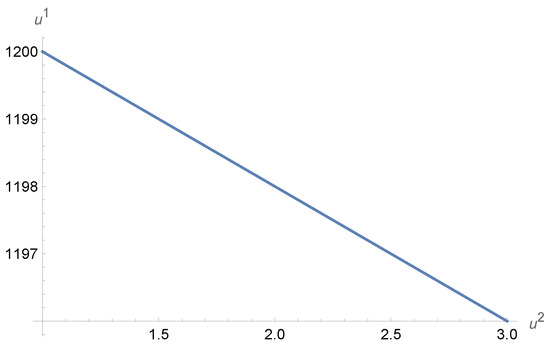
In the case of a small q compared with p, the system (21)–(23) becomes a slow–fast dynamical system with respect to slow time , in which and are fast variables, and is a slow one.
The theory of slow–fast dynamical systems, or singularly perturbed systems, has been actively developed since the last century and is presented in a wealth of papers and books; we refer to recent works with a fairly representative bibliography [22,23].
Such systems describe various physical phenomena in which a change in dynamic regimes is observed with a slow change in some of its variables. However, the (21)–(23) system does not show a variety of dynamic modes. This, in particular, is due to the non-hyperbolicity of the “slow curve” [22,23], which is obtained by equating the right-hand sides of Equations (21)–(23) to zero and is a set of points of the form , const, of the phase space of the system (21)–(23).
We construct an asymptotic solution for the system (21)–(23) accurate to by restricting ourselves to the leading term.
Let us search for a particular solution of Equation (27) accurate to in the form
where a smooth function does not depend on q.
From (23) and (27) with a given accuracy in q, we obtain
Approximate solutions of the system (21)–(23) can be found in the form of an expansion in q with an accuracy of :
Equations for obtained from (21)–(23) and (31) are
, , .
For more compact notation, we set , , , , , where is given in (26). Integration of system (32)–(36), subject to the conditions (26), yields
The geodesics in the coordinates of a local card of the space in the considered case are written as
They are obtained by integrating the relations with initial values , and for of the form (37)–(40) they are
In the case , the Riemann tensor (25) vanishes and the space is flat. In the coordinates of the local map , some components of the Christoffel symbols are zero (24). Hence, the coordinates are not Cartesian. The transition to Cartesian coordinates is given by
In the coordinates , the vector is given by the components that are as follows:
and the system (21)–(23) for the vector with reads
For , the coordinates are not Cartesian, and is not flat, because the Christoffel symbols (24) in these coordinates are nonzero, as are the components of the Riemann tensor.
Denote by the Christoffel symbols (24) in the coordinates . The non-zero are:
Equations (46) and (47) for geodesics in coordinates , according to (10), read
For , Equations (49) and (50) have a solution in the form of straight lines:
Equation (51) defines the geodesic flow in the flat .
In the case of , the numerical solutions of Equation (49) show that for various p and q and various initial conditions, for long times, after passing transient processes at short times, the solutions of Equation (49) behave as follows:
A typical example of such a solution is shown in Figure 2.
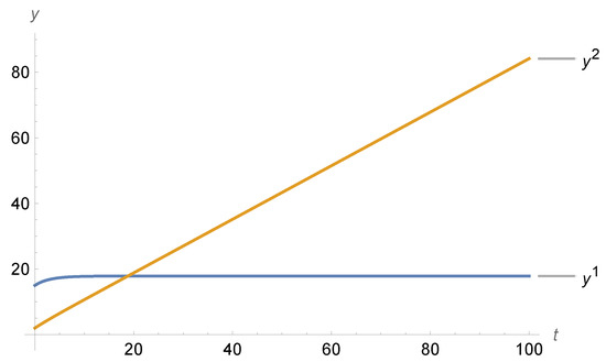
Figure 2.
The numerical solution of Equation (49) for , , , , .
The system (49), (50) for arbitrary p and q has the exact solution
where and are constant initial conditions for Equations (46), (47) and (49), (50), respectively. Then, from a comparison of (53) with numerical solutions, we can draw a conclusion that (48) is an attractor of geodesics in the space defined by (49) and (50) in the coordinates for .
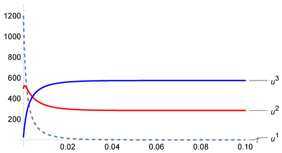
Passing to the original coordinates according to (44), we find that the solution of system (21)–(23) tends to the constant vector , , as , where the constant components and of depend on the initial vector and parameters . The quantities and can be obtained from two integrals given by (2) and (28), where the constants and are determined by the initial vector : , .
Figure 3 shows an example of the numerical solution of system (21)–(23) over a short time interval, where a transition to the stationary state is observed for the parameters and as in Figure 2, and the initial vector . Numerical solutions of system (1) were controlled using the integral (2).
For (), the system (14) is written as
Considering Equation (54) as defining the geodesic in the coordinate system , from the condition , by analogy with (21)–(23), we define the connection ∇ by the coefficients (12) for , whose explicit form we omit for simplicity reasons.
In the case of , the nonzero components of the Riemann tensor are equal to . We can directly verify the relation
Here, is the operator of covariant differentiation of the Riemann tensor R, and the covector has the form .
Then, the space becomes a recurrent affine space, which was introduced in [24,25]. The studies of these spaces showed their importance not only in the geometry and topology of manifolds, but also in physical applications such as gravity and field theory.
Analysis of the system (54) leads to results similar to the considered case .
The system (54) has the stationary solution
which can be regarded as an attractor of the system. Here, and are constant.
Numerical solutions of Equations (54) for various initial conditions and parameters show that there is a transition from the initial state to the stationary state as . This transition already occurs at rather short times. The typical behavior of solutions to system (54) is shown in Figure 4 for and , , , . The stationary state is .
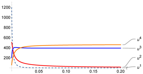
Figure 4.
The numerical solution of Equation (54).
From the considered examples, we can assume that the solutions of system (11) for an arbitrary N tend to the stationary solution asymptotically in t, , and some of the variables , , of the stationary solution are equal to zero.
In the generalizations of the theory of geodesic mappings of affinely connected spaces and Riemannian spaces, the definition of quasigeodesic [26,27] or F-planar curves (see, e.g., Ref. [18]) is introduced, which generalizes the notion of the geodesic curve.
The idea of the theory of geodesic mappings and its generalizations can be compiled from [17,18,19], where an extensive bibliography can also be found. In a torsion-free affine connection space with a tensor field F of the type (1,1), a curve is said to be quasigeodesic or F-planar (see [18,27] and references therein) if its tangent vector during parallel transport does not leave the domain formed by the tangent vector and the adjoint vector , i.e.,
where and are functions of t and is the covariant derivative along of (7).
For the case , the Smoluchowski Equation (1) with can be written as (57). We will consider it as the equation of the quasigeodesic in the sense of [26,27]. The nonzero components of the tensor F in the coordinate system are , , , , , , where due to the particle number conservation in the system. Equation (1) with the notations of the system (21)–(23) can be written as
The construction of analytical exact or approximate solutions of the system (58) for arbitrary parameters , and is non-trivial and makes sense for large N; this calls for separate study.
The system (58) for has the exact stationary solution , where is an arbitrary constant and
The stationary solution (59) can be regarded as an attractor of solutions to the system (58) with the given initial vector , and the parameter of (59) is determined using the integral (2) from the condition
which yields a cubic equation for .
Figure 5 shows an example of a numerical solution of the system for the values of the parameters , , , and initial conditions on a short time interval , where the transition to the exact stationary state can be observed.
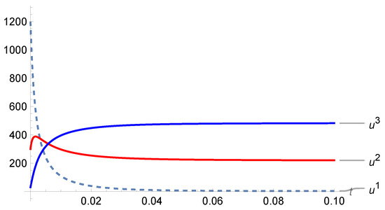
Figure 5.
The numerical solution of Equation (58).
5. Example: EDG Equation
Here, we look at the EDG Equation (13) as the geodesic Equation (10) with Christoffel symbols (14) for low dimensions N, by analogy with (11) in the previous section. Note that, by the definition of Equation (13) in accordance with [10], we can assume for a given N.
Let us consider the simplest nontrivial case, . For , , Equation (13) is written as
From (14), the nonzero symmetric Christoffel symbols are
For arbitrary parameters , the Riemann and Ricci tensors have a complex form.
In the case where , , , , the Riemann tensor vanishes, and the space with the connection (62) is flat. The dynamics of the system (61) can be explored using exact analytical solutions for , similarly to the system (21)–(23) discussed in Section 4. The influence of the parameters under the assumption when they are small can be taken into account through perturbation theory.
Numerical solutions of the system (61) show that, for different values of the parameters , the behavior of the solutions is qualitatively similar. A characteristic feature is the transition to stationary values of with increasing t. Figure 6 shows a typical example of such a solution for , , , with the initial condition .
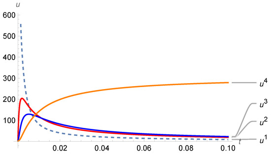
Figure 6.
The numerical solution of the system (61) for the parameters , , , with the initial condition .
As , the variables of the system (61) tend to the stationary solution for and . Here, is the integral (2) of the system (61) expressed in terms of the initial conditions: . Additionally, we assume that .
Figure 7 shows the solution of the system (61) for , , and , which corresponds to the case of a flat space . A comparison of Figure 6 and Figure 7 shows the similarity in the behavior of both solutions. However, in this case, for we have for , , and due to the last equation of the system (61).
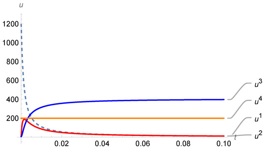
Figure 7.
The numerical solution of equations of the system (61) for , , with the initial condition .
Over a long time, the behavior of a solution , , to the system (13) with a given initial value for arbitrary N and , can be such that for , and .
6. Concluding Remarks
Mathematical models of the processes of aggregation and fragmentation of particles of various sizes and compositions have been developed and studied for over a century and continue to be a topical area of research. Because these processes are ubiquitous in natural phenomena at all spatial scales, from the micro to the macro level, they are a key element in understanding the patterns of specific phenomena.
In this paper, we use an approach in which binary kinetic equations are considered as equations of geodesics of an appropriate space with an affine connection. This makes it possible to describe kinetic processes in terms of the geodesic flows of the space associated with the kinetic equation.
The geometry of affine spaces has a long history and has by now accumulated a rich spectrum of ideas and methods that are used in numerous applications, especially in field theory and gravity, as partially presented in the bibliography below, e.g., Refs. [13,14,27], et al.
However, the spaces of affine connection introduced in this work and associated with binary kinetic equations are little studied, but may be of interest in various fields of condensed matter physics, as well as in biophysics. Some properties of the introduced spaces follow directly from their definition. In particular, such a space has the property that it has a coordinate system related to some local map, in which the connection is given by symmetric and constant Christoffel symbols defined by the kinetic equation. As a consequence, this space turns out to be equiaffine, and the volume element is conserved in it. As a preliminary study of these spaces, we have considered some of their obvious properties and toy examples of cases for . The transition to a stationary state over long times in these examples is natural due to the conservation of the number of particles in the system.
In this connection, we note the role of kinetics in describing the specific properties of highly dilute aqueous solutions and suspensions using fractal representations [8,28], as well as in the search for approaches to the study of a number of phenomena discovered experimentally that can be of interest as a means of construction of mathematical models.
In [8], using the kinetic Equation (1), and in [28], it was shown that in highly dilute solutions and suspensions, viscosity nonlinearly depends on concentration as a power law with an exponent associated with the fractal dimension. In our opinion, this indicates a correlation between kinetic phenomena and fractal properties in such systems. A detailed study of these objects is beyond the scope of this work and requires the use of new mathematical methods, among which fractal calculus seems to be the most promising (see [29] and references therein).
The specific properties of biologically active highly dilute substances called released-active forms (RA) have been discussed in [30,31]. Related issues have also been discussed in [32,33].
The physical basis of this phenomenon is currently not developed; therefore, various approaches are being tried, among which the fractality associated with the kinetics of particles in highly diluted substances ([34] and references therein) can become a prerequisite for features of the emergent behavior of such a system (e.g., Ref. [35]), which manifests itself in the specifics of its properties.
Funding
This research received no external funding.
Institutional Review Board Statement
Not applicable.
Informed Consent Statement
Not applicable.
Data Availability Statement
The data that support the findings of this study are available within the article.
Conflicts of Interest
The author declares no conflict of interest.
References
- Krapivsky, P.L. Aggregation processes with n-particle elementary reactions. J. Phys. A 1991, 24, 4697–4703. [Google Scholar] [CrossRef]
- Michel, P.; Benz, E.; Tanga, P.; Richardson, D.C. Collisions and gravitational reaccumulation: Forming asteroid families and satellites. Science 2001, 294, 1696–1700. [Google Scholar] [CrossRef] [PubMed]
- Sergei, D. Odintsov, S.D. Editorial for special issue feature papers 2020. Symmetry 2023, 15, 8. [Google Scholar]
- Brener, A. Model of many-particle aggregation in dense particle systems. Chem. Eng. Trans. 2014, 38, 145–150. [Google Scholar]
- von Smoluchowski, M. Drei vorträge über diffusion Brownsche molekular bewegung und koagulation von kolloidteichen. Phys. Z. 1916, 17, 557–571. [Google Scholar]
- Becker, R.; Döring, W. Kinetische behandlung der keimbildung in übersättigten dämpfen. Ann. Phys. 1935, 24, 719–752. [Google Scholar] [CrossRef]
- Ball, J.M.; Carr, J.; Penrose, O. The Becker-Döring cluster equations: Basic properties and asymptotic behaviour of solutions. Commun. Math. Phys. 1986, 104, 657–692. [Google Scholar] [CrossRef]
- Arinshtein, A.E. Effect of aggregation processes on the viscosity of suspensions. Sov. Phys. JETP 1992, 74, 646–649. [Google Scholar]
- van Dongen, P.G.J.; Ernst, M.H. Dynamic scaling in the kinetics of clustering. Phys. Rev. Lett. 1985, 54, 1396–1399. [Google Scholar] [CrossRef] [PubMed]
- Ben-Naim, E.; Krapivsky, P.L. Exchange-driven growth. Phys. Rev. E 2003, 68, 031104. [Google Scholar] [CrossRef]
- Esenturk, E. Mathematical theory of exchange-driven growth. Nonlinearity 2018, 31, 3460–3483. [Google Scholar] [CrossRef]
- Schlichting, A. The Exchange-driven growth model: Basic properties and longtime behavior. J. Nonlinear Sci. 2020, 30, 793–830. [Google Scholar] [CrossRef]
- Norden, A.P. Spaces with Affine Connection; Nauka: Moscow, Russia, 1976. [Google Scholar]
- Nomizu, K.; Sasaki, T. Affine Differential Geometry; Cambridge University Press: Cambridge, UK, 1994. [Google Scholar]
- Ballman, W. Lectures on Differential Geometry. Connections and Geodesics. Connections on Manifolds, Geodesics, Exponential Map. 2002. Available online: http://people.mpim-bonn.mpg.de/hwbllmnn/notes.html (accessed on 14 October 2022).
- Ballmann, W. Introduction to Geometry and Topology; Springer: Basel, Switzerland, 2015. [Google Scholar]
- Berezovski, V.E.; Mikeš, J. Almost geodesic mappings of spaces with affine connection. J. Math. Sci. 2015, 207, 389–409. [Google Scholar] [CrossRef]
- Mikeš, J.; Berezovski, V.E.; Stepanova, E.; Chudá, H. Geodesic mappings and their generalizations. J. Math. Sci. 2016, 217, 607–623. [Google Scholar] [CrossRef]
- Berezovski, V.; Cherevko, Y.; Hinterleitner, I.; Peška, P. Geodesic mappings of spaces with affine connections onto generalized symmetric and Ricci-symmetric spaces. Mathematics 2020, 8, 1560. [Google Scholar] [CrossRef]
- Lorenz, E.N. Deterministic nonperiodic flow. J. Atmos. Sci. 1963, 20, 130–141. [Google Scholar] [CrossRef]
- Rössler, O.E. An equation for continuous chaos. Phys. Lett. A 1976, 57, 397–398. [Google Scholar] [CrossRef]
- Benoît, E.; Brøns, M.; Desroches, M.; Krupa, M. Extending the zero-derivative principle for slow-fast dynamical systems. Z. Angew. Math. Phys. 2015, 66, 2255–2270. [Google Scholar] [CrossRef]
- Ginoux, J.-M. Slow invariant manifolds of slow-fast dynamical systems. Int. J. Bifurc. Chaos 2020, 31, 2150112. [Google Scholar] [CrossRef]
- Ruse, H.S. On simply harmonic spaces. J. Lond. Math. Soc. 1946, 21, 243–247. [Google Scholar] [CrossRef]
- Walker, A.G. On Ruse’s spaces of recurrent curvature. Proc. Lond. Math. Soc. 1950, 52, 36–64. [Google Scholar] [CrossRef]
- Petrov, A.Z. Modeling of physical fields. Gravit. Gen. Relat. Kazan Univ. 1968, 4–5, 7–21. (In Russian) [Google Scholar]
- Petrov, A.Z. Modeling of test-body paths in the gravitation field. Dokl. Akad. Nauk SSSR 1969, 186, 1302–1305. (In Russian) [Google Scholar]
- Oikonomou, V.K. On non-linear behavior of viscosity in low-concentration solutions and aggregate structures. Symmetry 2018, 10, 368. [Google Scholar] [CrossRef]
- Golmankhaneh, A.K. Fractal Calculus and Its Applications Fα-Calculus; World Scientific: Singapore, 2022. [Google Scholar]
- Epstein, O. The Spatial homeostasis hypothesis. Symmetry 2018, 10, 103. [Google Scholar] [CrossRef]
- Tarasov, S.A.; Gorbunov, E.A.; Don, E.S.; Emelyanova, A.G.; Kovalchuk, A.L.; Yanamala, N.; Schleker, A.S.S.; Klein-Seetharaman, J.; Groenestein, R.; Tafani, J.-P.; et al. Insights into the mechanism of action of highly diluted biologics. J. Immunol. 2020, 205, 1345–1354. [Google Scholar] [CrossRef]
- Shapovalov, A.V.; Obukhov, V.V. Some aspects of nonlinearity and self-organization in biosystems on examples of localized excitations in the DNA molecule and generalized Fisher–KPP model. Symmetry 2018, 10, 53. [Google Scholar] [CrossRef]
- Shapovalov, A.V.; Trifonov, A.Y. Approximate solutions and symmetry of a two-component nonlocal reaction-diffusion population model of the Fisher–KPP type. Symmetry 2019, 11, 366. [Google Scholar] [CrossRef]
- Brevik, I.; Shapovalov, A.V. Effects of low concentration in aqueous solutions within the fractal approach. Russ. Phys. J. 2022, 65, 197–207. [Google Scholar] [CrossRef]
- Seely, A.J.E.; Peter Macklem, P. Fractal variability: An emergent property of complex dissipative systems. Chaos 2012, 22, 013108. [Google Scholar] [CrossRef]
Disclaimer/Publisher’s Note: The statements, opinions and data contained in all publications are solely those of the individual author(s) and contributor(s) and not of MDPI and/or the editor(s). MDPI and/or the editor(s) disclaim responsibility for any injury to people or property resulting from any ideas, methods, instructions or products referred to in the content. |
© 2023 by the author. Licensee MDPI, Basel, Switzerland. This article is an open access article distributed under the terms and conditions of the Creative Commons Attribution (CC BY) license (https://creativecommons.org/licenses/by/4.0/).