A Generalised Time-Dependent Mathematical Formulation for Magnetoelectrically Coupled Soft Solids at Finite Strains

Abstract

To date, the mechanical models of magnetoelectric couplings at finite strains have mainly been limited to time-independent constitutive equations. This paper enhances the literature by developing a time-dependent electromagnetic constitutive equation to characterise the mechanical behaviour of soft solids at finite strains and take into account the full form of the Maxwell equations. Our formulation introduces a symmetrical total stress and uses recently developed spectral invariants in the amended energy function; as a result, the proposed constitutive equation is relatively simple and is amenable to a finite-element formulation.

1. Introduction

Research in the areas of so-called smart and multifunctional materials has grown exponentially in recent years. Smart materials can be defined as the innovative substances that can alter their physical and mechanical attributes when exposed to one or more external stimuli. Some widely used external stimuli are temperature, humidity, light, pH, and acoustic, electric, and magnetic fields [1,2]. Among other smart materials, electroactive polymers (EAPs) and magnetoactive polymers (MAPs) have received unprecedented attention in recent years thanks to their myriad of potential applications. These ever-expanding applications have reached many areas, including soft robotics for targeted drug delivery and cancer therapy, flexible stretch-based sensors for wearable devices, materials for morphing and shape-shifting structures, key ingredients for rapidly expanding metamaterials, to mention a few [1,2,3,4,5]. For EAPs, while working as the so-called dielectric elastomers (DEs), an electric voltage applied along the thickness direction of a thin structure will create Coulomb forces as a result of the attractions of two opposite charges resulting in expansions in the lateral directions [5]. This mechanism of converting electric input to a mechanical output is the key in actuators for soft robotics. Furthermore, EAPs can be used in energy harvesting using ambient motions, in which a mechanical input creates electric outputs that could be the essential ingredients for creating clean and green sustainable energy.

In MAPs, a polymeric composite filled with magnetisable particles (micro or nanosized) can be activated upon the application of a remotely controlled magnetic field. Depending on the filler particles, MAPs can be decomposed into two groups, i.e., soft-magnetic MAPs, where particles have less residual magnetisation and coercivity, while in hard-magnetic MAPs, particles retain a high coercivity with a significant remanence magnetisation after the removal of the external magnetic field, see, for example, reference [6]. Note that soft-magnetic MAPs are mainly used in areas where mechanical properties such shear and loss moduli are to be tuned, while for applications in largely deformable and flexible shape-shifting structures, hard-magnetic MAPs are used. For various matrix materials, fillers, manufacturing techniques, experimental characterisations, and the computational modelling of both hard and soft MAPs, a few recent review papers can be consulted, see, for example, [6].

The experimental study, mathematical modelling and simulations, and the search for novel applications of EAPs and MAPs have so far been performed separately. However, very recently, following the so-called multiferroic materials in which a magnetoelectric coupling occurs simultaneously, the quest for largely deformable similar materials has increased manifolds where magnetoelectric coupling is a common phenomenon. Note that ceramic and metal-based magneto-electroactive hard materials have applications in producing magnetoelectric random access memories [7,8]. An interesting counterpart to these hard materials could be a soft polymeric material (elastomer or hydrogel), in which a polymeric matrix is filled with magnetisable (e.g., iron, neodymium–iron–boron) particles [9,10]. A typical application of such material is in hyperthermia for cancer patients, in which a remotely controlled dynamic magnetic field will create localised heat as a result of vibrating particles in a conductive polymeric matrix. All these nascent applications require the development of appropriate mathematical frameworks to simulate magnetoelectric coupling phenomena at finite strains.

Until recently, the mathematical modelling of magnetoelectric couplings at finite strains has been limited, in the sense that models have discarded the time-dependence of the electro-magneto-mechanically coupled problems in formulating the governing equations. In this contribution, we aim to present a generalised mathematical formulation for magnetoelectrically coupled soft materials at finite strains that takes into account time-dependent dynamical phenomena. Following our recent works [11,12] on electromagnetic–elastic materials including the modelling of residual stresses appearing in magnetoelectric elasticity, we briefly present the relevant and key governing equations that are essential to represent a magneto-electro-mechanically coupled system at large strains. Afterwards, the framework is extended to incorporate the time-dependent dynamical aspects. Finally, we use an attractive set of spectral invariants [12] to mechanically characterise the proposed amended energy function.

1.1. Remark

There are many coexisting theories and results on the subject of electromagnetic continuum mechanics theory. The physics and mathematics of electromagnetic forces in continuum mechanics are complex and tedious, and it is beyond the scope of this paper to regurgitate them here. Readers are encouraged to read references [13,14,15] for the basic concepts of electromagnetic forces in deformable continua. In this paper, we only focus on a mathematical construction (which uses some fundamental equations and concepts for a solid continuum in the presence of electromagnetic fields based on the work of references [13,14,15]) to provide a relatively simple form of constitutive equation, which is beneficial to obtain boundary value problem results (especially with the aid of the finite element method) and for design purposes. We believe the mathematical construction and proofs developed in this article are not found in the literature and hence could be employed for future research.

An attractive set of spectral invariants and their derivatives are used in our proposed model; readers may not be familiar with them and their physical concept, since their development are only recent; see for example, references [16,17,18]. The concept and derivation of spectral models are rather involved, and hence it is beyond the scope of this paper to repeat them here. Readers are encouraged to read references [16,17,18] and references therein, for details on spectral modelling.

1.2. Kinematics

The descriptions of the deformation tensor $\mathbf{F}$, the right-stretch tensor $\mathbf{U}$, right Cauchy–Green tensor $\mathbf{C}={\mathbf{U}}^2$, and scalar $J=det\mathbf{F}>0$, where det denotes the determinant of a tensor, can be found in Ogden [19]. Unless stated otherwise, in this paper, all subscripts $i,j$, and k take the values one, two, and three.

1.3. Electromagnetic Field Equations

Here, we briefly state some fundamental equations and concepts for a solid continuum in the presence of electromagnetic fields based on the work of references [13,14,15].

1.3.1. Maxwell Equations

We use the notation $q_{\mathrm{e}}$ for the density of electric charge per unit of volume and $\mathbb{J}$ for the volume electric current. In the case $q_{\mathrm{e}}=0$ and $\mathbb{J}=\mathbf{0}$, the Maxwell equations are (see [13,15]):

$$\mathrm{div}\mathbb{B}=0,\mathrm{curl}\mathbb{E}+\dot{\mathbb{B}}=\mathbf{0},\mathrm{div}\mathbb{D}=0,\mathrm{curl}\mathbb{H}=\dot{\mathbb{D}},$$

(1)

where $\mathbb{B}$ is the magnetic induction, $\mathbb{E}$ is the electric field, $\mathbb{D}$ is the electric displacement, $\mathbb{H}$ is the magnetic field, and $\dot{\left(\right)}$ is the time derivative keeping $\mathbf{x}$ constant, i.e., for example ${\displaystyle \dot{\mathbb{B}}=\frac{\partial \mathbb{B}(\mathbf{x},t)}{\partial t}}$, $div$ and $curl$ are the divergence and curl operators in the current configuration.

For a vacuum, the following relations between the electric variables and the magnetic variables are:

$$\mathbb{D}={\epsilon }_{\mathrm{o}}\mathbb{E},\mathbb{B}={\mu }_{\mathrm{o}}\mathbb{H},$$

(2)

where ${\epsilon }_{\mathrm{o}}$ is the electric permittivity in vacuum, and ${\mu }_{\mathrm{o}}$ is the magnetic permeability in vacuum. For a condensed matter two extra fields can be defined, which are the electric polarization $\mathbb{P}$ and the magnetization $\mathbb{M}$, i.e.,

$$\mathbb{D}={\epsilon }_{\mathrm{o}}\mathbb{E}+\mathbb{P},\mathbb{B}={\mu }_{\mathrm{o}}(\mathbb{H}+\mathbb{M}),$$

(3)

1.3.2. Lagrangian Electric and Magnetic Variables

From [14,20,21] the expressions for the electric and the magnetic variables in the reference configuration are

$${\mathbb{E}}_{\mathrm{L}}={\mathbf{F}}^{\mathrm{T}}\mathbb{E},{\mathbb{D}}_{\mathrm{L}}=J{\mathbf{F}}^{-1}\mathbb{D},{\mathbb{B}}_{\mathrm{L}}=J{\mathbf{F}}^{-1}\mathbb{B},{\mathbb{H}}_{\mathrm{L}}={\mathbf{F}}^{\mathrm{T}}\mathbb{H}.$$

(4)

1.3.3. Continuity Conditions

The imposition of boundary conditions in electromagnetic boundary value problems is not trivial, due to the requirement of Maxwell Equation (1) to be satisfied in the body and also for the exterior surrounding, which is assumed to be a vacuum space. To make the boundary conditions clear (see also Figure 1), we introduce the notation

$$\begin{array}{c}\hfill \left[\left[a\right]\right]=a^{\left(\mathrm{o}\right)}-a^{\left(\mathrm{i}\right)},\end{array}$$

(5)

where (o) is associated with the outside of the body and (i) is associated with the inside of the body, which is very close to the surface of the body. The boundary conditions for the electromagnetic fields require the following continuity conditions [14]

$$\mathbf{n}·\left[\left[\mathbb{B}\right]\right]=0,\mathbf{n}\times \left[\left[\mathbb{E}\right]\right]=v_{\mathrm{n}}\left[\left[\mathbb{B}\right]\right],\mathbf{n}·\left[\left[\mathbb{D}\right]\right]=q_{\mathrm{e}}^{\mathrm{S}},\mathbf{n}\times \left[\left[\mathbb{H}\right]\right]+v_{\mathrm{n}}\left[\left[\mathbb{D}\right]\right]={\mathbb{J}}^{\mathrm{S}},$$

(6)

where $v_{\mathrm{n}}=\mathbf{v}·\mathbf{n}$ is the normal component of the velocity field, $\mathbf{n}$ is the outward unitary normal vector to $\partial {\mathcal{B}}_t$ (the surface of the body in the current configuration), $q_{\mathrm{e}}^{\mathrm{S}}$ represents a surface distribution of free charges, and ${\mathbb{J}}^{\mathrm{S}}$ is a surface distribution of the electric current. From now on, we assume that $q_{\mathrm{e}}^{\mathrm{S}}=0$ and ${\mathbb{J}}^{\mathrm{S}}=\mathbf{0}$.

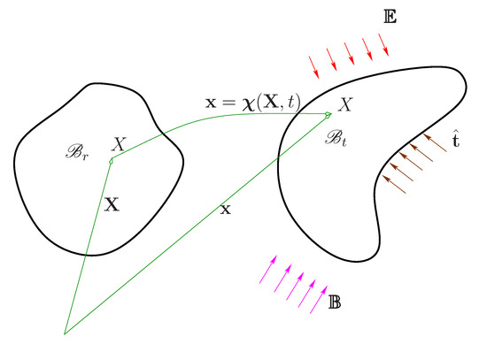
Figure 1. Deformation due to the application of electromagnetic fields $\mathbb{B}$ and $\mathbb{E}$, boundary displacement, and boundary traction $\widehat{\mathbf{t}}$. ${\mathcal{B}}_r$ is the reference (undeformed) configuration, ${\mathcal{B}}_t$ is the current configuration, and X and x are, respectively, the position vectors of X in the reference and current configurations, where X represents a generic particle of the solid body.

At the boundary, the generally nonsymmetric Cauchy stress tensor $\sigma$ satisfies the continuity condition

$$\left[[\sigma -{\sigma }_{\mathrm{M}}]\right]\mathbf{n}=\widehat{\mathbf{t}},$$

(7)

where $\widehat{\mathbf{t}}$ is the external mechanical traction and the Maxwell stress tensor ${\sigma }_{\mathrm{M}}$ has the relation [13,14]

$${\sigma }_{\mathrm{M}}=\frac{1}{2}\left({\epsilon }_o\mathbb{E}·\mathbb{E}+\frac{1}{{\mu }_o}\mathbb{B}·\mathbb{B}-2\mathbb{M}·\mathbb{B}\right)\mathbf{I}-\left({\epsilon }_o\mathbb{E}\otimes \mathbb{E}+\mathbb{P}\otimes \mathbb{E}+\frac{1}{{\mu }_o}\mathbb{B}\otimes \mathbb{B}-\mathbb{B}\otimes \mathbb{M}\right).$$

(8)

1.4. Balance of Mass and Equation of Motion

The mass balance equation is [19]

$$\begin{array}{c}\hfill \dot{\rho }+\mathrm{div}\left(\rho \mathbf{v}\right)=0,\end{array}$$

(9)

where $\mathbf{v}$ is the velocity and $\rho$ is the density of the body. The density in the reference configuration is denoted ${\rho }_{\mathrm{r}}$ and $\rho =J^{-1}{\rho }_{\mathrm{r}}$.

The first law of movement is [13]

$$\rho \frac{\mathrm{D}\mathbf{v}}{\mathrm{D}t}=div\sigma +{\mathbf{f}}_{\mathrm{e}}+\mathbf{f},$$

(10)

where ${\displaystyle \frac{\mathrm{D}\mathbf{v}}{\mathrm{D}t}}$ is the acceleration and ${\displaystyle \frac{\mathrm{D}}{\mathrm{D}t}}$ is the total time derivative, ${\mathbf{f}}_{\mathrm{e}}$ is the body force due to the electromagnetic interactions and $\mathbf{f}$ is the body force that is independent of the electromagnetic fields. In the case $q_{\mathrm{e}}=0$ and $\mathbb{J}=\mathbf{0}$, the body force ${\mathbf{f}}_{\mathrm{e}}$ is given by [13]

$${\mathbf{f}}_{\mathrm{e}}={\left(grad\mathbb{E}\right)}^{\mathrm{T}}\mathbb{P}+{\left(grad\mathbb{B}\right)}^{\mathrm{T}}\mathbb{M}+\dot{\overline{\mathbb{P}\times \mathbb{B}}}+div[\mathbf{v}\otimes (\mathbb{P}\times \mathbb{B})].$$

(11)

The second law of movement is stated as

$$\begin{array}{c}\hfill ϵ\sigma =\mathbf{L},\end{array}$$

(12)

where $\mathbf{\sigma }$ is the Cauchy stress tensor. It is clear from Equation (12) that if the vector field $\mathbf{L}\ne 0$, then the Cauchy stress $\sigma$ is a nonsymmetric second-order tensor. We note that $ϵ$ is the permutation tensor and, in this paper, we use the operator

$$\begin{array}{c}\hfill ϵ(\mathbf{b}\otimes \mathbf{c})=\mathbf{c}\times \mathbf{b},\end{array}$$

(13)

where $\mathbf{b}$ and $\mathbf{c}$ are vectors.

2. Constitutive Equations

2.1. The Amended Energy Function and the Total Stress Tensor

If $\psi$ is the Helmholtz potential and $\psi =\psi (\mathbf{F},{\mathbb{E}}^{\mathrm{e}},\mathbb{B})$ [13,14]), we have, for an isothermal problem, the Clausius–Duhem inequality, which takes the form

$$\begin{array}{c}\hfill \mathbf{\sigma }:\mathbf{D}-\rho \dot{\psi }-{\mathbb{M}}^{\mathrm{e}}·\dot{\mathbb{B}}-{\dot{\mathbb{E}}}^{\mathrm{e}}·\mathbb{P}\ge 0,\end{array}$$

(14)

where the superposed dot represents the time derivative, : denotes the inner product of two second-order tensors, and $\mathbf{D}=grad\mathbf{v}$. In view of the relation $\mathbf{\sigma }:\mathbf{D}={\left({\mathbf{F}}^{-1}\mathbf{\sigma }\right)}^{\mathrm{T}}:\dot{\mathbf{F}}$, (14) takes the form

$$\begin{array}{c}\hfill {\left({\mathbf{F}}^{-1}\mathbf{\sigma }-\rho {\displaystyle \frac{\partial \psi }{\partial \mathbf{F}}}\right)}^{\mathrm{T}}:\dot{\mathbf{F}}-\left(\rho {\displaystyle \frac{\partial \psi }{\partial \mathbb{B}}}+{\mathbb{M}}^{\mathrm{e}}\right)·\dot{\mathbb{B}}-\left(\rho {\displaystyle \frac{\partial \psi }{\partial {\mathbb{E}}^{\mathrm{e}}}}+\mathbb{P}\right)·{\dot{\mathbb{E}}}^{\mathrm{e}}\ge 0.\end{array}$$

(15)

Since $\dot{\mathbf{F}}$, $\dot{\mathbb{B}}$, and ${\dot{\mathbb{E}}}^{\mathrm{e}}$ are arbitrary, we obtain the relations

$$\sigma =\rho \mathbf{F}\frac{\partial \psi }{\partial \mathbf{F}},\mathbb{P}=-\rho \frac{\partial \psi }{\partial {\mathbb{E}}^{\mathrm{e}}},{\mathbb{M}}^{\mathrm{e}}=-\rho \frac{\partial \psi }{\partial \mathbb{B}},$$

(16)

where

$${\mathbb{E}}^{\mathrm{e}}=\mathbb{E}+\overline{\mathbb{E}},\overline{\mathbb{E}}=\mathbf{v}\times \mathbb{B},{\mathbb{M}}^{\mathrm{e}}=\mathbb{M}+\overline{\mathbb{M}},\overline{\mathbb{M}}=\mathbf{v}\times \mathbb{P}.$$

(17)

and we use the convention ${\displaystyle {\left(\frac{\partial \psi }{\partial \mathbf{F}}\right)}_{\alpha i}=\frac{\partial \psi }{\partial F_{i\alpha }}}$ [19].

In order to define a “total symmetric stress tensor”, let us consider the following relations. First, notice that from Equation(1) and (3) we have

$$\mathrm{div}\left(\mathbb{D}\otimes \mathbb{E}\right)=\left(\mathrm{grad}\mathbb{E}\right)\mathbb{D}={\epsilon }_o\left(\mathrm{grad}\mathbb{E}\right)\mathbb{E}+\left(\mathrm{grad}\mathbb{E}\right)\mathbb{P},\mathrm{div}\left[\frac{\left(\mathbb{E}·\mathbb{E}\right)}{2}\mathbf{I}\right]={\left(grad\mathbb{E}\right)}^{\mathrm{T}}\mathbb{E}.$$

(18)

Using the relations

$$\left[\left(\mathrm{grad}\mathbb{E}\right)-{\left(\mathrm{grad}\mathbb{E}\right)}^{\mathrm{T}}\right]\mathbb{E}=\mathrm{curl}\mathbb{E}\times \mathbb{E},\left[\left(\mathrm{grad}\mathbb{E}\right)-{\left(grad\mathbb{E}\right)}^{\mathrm{T}}\right]\mathbb{P}=\mathrm{curl}\mathbb{E}\times \mathbb{P},$$

(19)

we have

$$\mathrm{div}\left[\mathbb{D}\otimes \mathbb{E}-\frac{1}{2}{\epsilon }_o\left(\mathbb{E}·\mathbb{E}\right)\mathbf{I}\right]={\left(\mathrm{grad}\mathbb{E}\right)}^{\mathrm{T}}\mathbb{P}+\mathrm{curl}\mathbb{E}\times \mathbb{P}+{\epsilon }_o\mathrm{curl}\mathbb{E}\times \mathbb{E}.$$

(20)

In view of (1), we have the relation $\mathrm{curl}\mathbb{E}=-\dot{\mathbb{B}}$ and from (18), we obtain

$$\mathrm{div}\left[\mathbb{D}\otimes \mathbb{E}-\frac{1}{2}{\epsilon }_o\left(\mathbb{E}·\mathbb{E}\right)\mathbf{I}\right]={\left(\mathrm{grad}\mathbb{E}\right)}^{\mathrm{T}}\mathbb{P}-\dot{\mathbb{B}}\times \mathbb{P}-{\epsilon }_o\dot{\mathbb{B}}\times \mathbb{E}={\left(\mathrm{grad}\mathbb{E}\right)}^{\mathrm{T}}\mathbb{P}-\dot{\mathbb{B}}\times \mathbb{D},$$

(21)

thus

$${\left(\mathrm{grad}\mathbb{E}\right)}^{\mathrm{T}}\mathbb{P}=\mathrm{div}\left[\mathbb{D}\otimes \mathbb{E}-\frac{{\epsilon }_o}{2}(\mathbb{E}·\mathbb{E})\mathbf{I}\right]+\dot{\mathbb{B}}\times \mathbb{D}.$$

(22)

On the other hand, using the relations

$$\begin{array}{ccc}& & \mathrm{div}\left(\mathbb{B}\otimes \mathbb{B}\right)=\left(\mathrm{grad}\mathbb{B}\right)\mathbb{B},\mathrm{div}\left[\frac{\left(\mathbb{B}·\mathbb{B}\right)}{2}\mathbf{I}\right]={\left(\mathrm{grad}\mathbb{B}\right)}^{\mathrm{T}}\mathbb{B},\hfill \end{array}$$

(23)

$$\begin{array}{ccc}& & \left[\left(\mathrm{grad}\mathbb{B}\right)-{\left(\mathrm{grad}\mathbb{B}\right)}^{\mathrm{T}}\right]\mathbb{B}=\mathrm{curl}\mathbb{B}\times \mathbb{B},\hfill \end{array}$$

(24)

we have, in view of (1) and (3):

$$\frac{1}{{\mu }_o}\mathrm{div}\left[\mathbb{B}\otimes \mathbb{B}-\frac{\left(\mathbb{B}·\mathbb{B}\right)}{2}\mathbf{I}\right]=\frac{1}{{\mu }_o}\mathrm{curl}\mathbb{B}\times \mathbb{B}=\dot{\mathbb{D}}\times \mathbb{B}+\left(curl\mathbb{M}\right)\times \mathbb{B}.$$

(25)

Therefore, from (1), we have the relations

$$\mathrm{div}\left[\left(\mathbb{M}·\mathbb{B}\right)\mathbf{I}\right]={\left(\mathrm{grad}\mathbb{B}\right)}^{\mathrm{T}}\mathbb{M}+{\left(\mathrm{grad}\mathbb{M}\right)}^{\mathrm{T}}\mathbb{B},\mathrm{div}\left(\mathbb{B}\times \mathbb{M}\right)=\left(\mathrm{grad}\mathbb{M}\right)\mathbb{B}.$$

(26)

Using the relation

$$\left[\mathrm{grad}\mathbb{M}-{\left(grad\mathbb{M}\right)}^{\mathrm{T}}\right]\mathbb{B}=\mathrm{curl}\mathbb{M}\times \mathbb{B},$$

(27)

we obtain

$$\mathrm{div}\left[\left(\mathbb{M}·\mathbb{B}\right)\mathbf{I}-\mathbb{B}\otimes \mathbb{M}\right]={\left(\mathrm{grad}\mathbb{B}\right)}^{\mathrm{T}}\mathbb{M}-\left(curl\mathbb{M}\right)\times \mathbb{B}.$$

(28)

and from (25) and (28), we have

$${\left(\mathrm{grad}\mathbb{B}\right)}^{\mathrm{T}}\mathbb{M}=\mathrm{div}\left\{\frac{1}{{\mu }_o}\left[\mathbb{B}\otimes \mathbb{B}-\frac{1}{2}\left(\mathbb{B}·\mathbb{B}\right)\mathbf{I}\right]+\left(\mathbb{M}·\mathbb{B}\right)\mathbf{I}-\mathbb{B}\otimes \mathbb{M}\right\}-\dot{\mathbb{D}}\times \mathbb{B}.$$

(29)

To facilitate our formulation, we let

$$\psi (\mathbf{F},{\mathbb{E}}^{\mathrm{e}},\mathbb{B})=\psi \left(\mathbf{F},{\mathbf{F}}^{-\mathrm{T}}{\mathbb{E}}_{\mathrm{L}}^{\mathrm{e}},\frac{1}{J}\mathbf{F}\mathbb{B}\right)=\varphi (\mathbf{U},{\mathbb{B}}_{\mathrm{L}},{\mathbb{E}}_{\mathrm{L}}^{\mathrm{e}}),$$

(30)

where

$${\mathbb{E}}_{\mathrm{L}}^{\mathrm{e}}={\mathbf{F}}^{\mathrm{T}}{\mathbb{E}}^{\mathrm{e}}.$$

(31)

We note that $\varphi$ is objective [19]. Consider the relations

$$\frac{\partial {\mathbb{E}}^{\mathrm{e}}}{\partial \mathbf{F}}=-{\mathbf{F}}^{-\mathrm{T}}\otimes {\mathbb{E}}^{\mathrm{e}},\frac{\partial \mathbb{B}}{\partial \mathbf{F}}=-\frac{1}{J}\left(-\mathbf{F}{\mathbb{B}}_{\mathrm{L}}\otimes {\mathbf{F}}^{-1}+\sum _{i=1}^3{\mathbf{e}}_i\otimes {\mathbb{B}}_{\mathrm{L}}\otimes {\mathbf{e}}_i\right),$$

(32)

where $\left\{{\mathbf{e}}_i\right\}$ is the unit orthogonal vector basis in Cartesian coordinates in the current configuration.

Using the previous expressions in (16), we prove that

$$\sigma =2\rho \mathbf{F}\frac{\partial \varphi }{\partial \mathbf{C}}{\mathbf{F}}^{\mathrm{T}}-\mathbb{P}\otimes {\mathbb{E}}^{\mathrm{e}}-\left({\mathbb{M}}^{\mathrm{e}}·\mathbb{B}\right)\mathbf{I}+\mathbb{B}\otimes {\mathbb{M}}^{\mathrm{e}}.$$

(33)

Proof. 

From (30) (see (31) and (4)) and using the chain rule, we obtain,

$$\mathbf{F}\frac{\partial \varphi }{\partial \mathbf{F}}=\mathbf{F}\left(\frac{\partial \psi }{\partial \mathbf{F}}+\frac{\partial \psi }{\partial \mathbb{B}}\frac{\partial \mathbb{B}}{\partial \mathbf{F}}+\frac{\partial \psi }{\partial {\mathbb{E}}^{\mathrm{e}}}\frac{\partial {\mathbb{E}}^{\mathrm{e}}}{\partial \mathbf{F}}\right).$$

(34)

The mathematical derivations below require the operator

$$\mathbf{q}(\mathbf{r}\otimes \mathbf{s}\otimes \mathbf{w})=(\mathbf{q}·\mathbf{r})(\mathbf{s}\otimes \mathbf{w}),$$

(35)

where $\mathbf{q}$, $\mathbf{r}$, $\mathbf{s}$, and $\mathbf{w}$ are vectors. From (16), we have

$$\rho \mathbf{F}\frac{\partial \psi }{\partial \mathbf{F}}=2\rho \mathbf{F}\frac{\partial \varphi }{\partial \mathbf{C}}{\mathbf{F}}^{\mathrm{T}}=\sigma -\left(\mathbf{F}{\mathbb{M}}^{\mathrm{e}}\right)\frac{\partial \mathbb{B}}{\partial \mathbf{F}}-\left(\mathbf{F}\mathbb{P}\right)\frac{\partial {\mathbb{E}}^{\mathrm{e}}}{\partial \mathbf{F}},$$

(36)

and using (35), we obtain,

$$2\rho \mathbf{F}\frac{\partial \varphi }{\partial \mathbf{C}}{\mathbf{F}}^{\mathrm{T}}=\sigma -\left(\mathbf{F}{\mathbb{M}}^{\mathrm{e}}\right)\frac{1}{J}\left(-\mathbf{F}{\mathbb{B}}_{\mathrm{L}}\otimes {\mathbf{F}}^{-1}+\sum _{i=1}^3{\mathbf{e}}_i\otimes {\mathbb{B}}_{\mathrm{L}}\otimes {\mathbf{e}}_i\right)+\left(\mathbf{F}\mathbb{P}\right){\mathbf{F}}^{-\mathrm{T}}\otimes {\mathbb{E}}^{\mathrm{e}}.$$

(37)

We then obtain the simplified form

$$2\rho \mathbf{F}\frac{\partial \varphi }{\partial \mathbf{C}}{\mathbf{F}}^{\mathrm{T}}=\sigma +\left({\mathbb{M}}^{\mathrm{e}}·\mathbb{B}\right)\mathbf{I}-\mathbb{B}\otimes {\mathbb{M}}^{\mathrm{e}}+\mathbb{P}\otimes {\mathbb{E}}^{\mathrm{e}},$$

(38)

which implies that ${\displaystyle \sigma =2\rho \mathbf{F}\frac{\partial \varphi }{\partial \mathbf{C}}{\mathbf{F}}^{\mathrm{T}}-\mathbb{P}\otimes {\mathbb{E}}^{\mathrm{e}}-\left({\mathbb{M}}^{\mathrm{e}}·\mathbb{B}\right)\mathbf{I}+\mathbb{B}\otimes {\mathbb{M}}^{\mathrm{e}}}$. □

We prove that $\mathbb{P}\otimes \left(\mathbf{v}\times \mathbb{B}\right)=\mathbb{B}\otimes \overline{\mathbb{M}}-\left(\overline{\mathbb{M}}·\mathbb{B}\right)\mathbf{I}+\mathbf{v}\otimes \left(\mathbb{P}\times \mathbb{B}\right)$. Considering Cartesian coordinates, let

$$\mathbf{A}=\mathbb{P}\otimes \left(\mathbf{v}\times \mathbb{B}\right)\iff A_{ij}={\mathbb{P}}_i{ϵ}_{irs}{v}_r{b}_s,$$

and

$$\begin{array}{ccc}& & \mathbf{G}=\mathbb{B}\otimes \overline{\mathbb{M}}-\left(\overline{\mathbb{M}}·\mathbb{B}\right)\mathbf{I}+\mathbf{v}\otimes \left(\mathbb{P}\times \mathbb{B}\right)\hfill \\ & & \iff G_{ij}={\mathbb{B}}_i{ϵ}_{jrs}{v}_r{\mathbb{P}}_s-{ϵ}_{krs}{v}_r{\mathbb{P}}_s{\mathbb{B}}_k{\delta }_{ij}+v_i{ϵ}_{jrs}{\mathbb{P}}_r{\mathbb{B}}_s.\hfill \end{array}$$

For the case $i\ne j$, in particular when $i=1$ and $j=2$, we have

$$A_{12}={\mathbb{P}}_1{ϵ}_{213}{v}_1{\mathbb{B}}_3+{\mathbb{P}}_1{ϵ}_{231}{v}_3{\mathbb{B}}_1=G_{12},$$

and the same results can be obtained for $(i,j)=(1,3)$, $(i,j)=(2,1)$, etc., then for $i\ne j$, we have that $A_{ij}=G_{ij}$. For the case $i=j$, for example when $i=j=1$, we have

$$A_{11}={\mathbb{P}}_1{ϵ}_{123}{v}_2{\mathbb{B}}_3+{\mathbb{P}}_1{ϵ}_{132}{v}_3{\mathbb{B}}_2=G_{11},$$

and similar results are obtained for the cases $i=j=2$ and $i=j=3$.

Using the relation

$$\mathbb{P}\otimes (\mathbf{v}\times \mathbb{B})=\mathbb{B}\otimes \overline{\mathbb{M}}-\left(\overline{\mathbb{M}}·\mathbb{B}\right)\mathbf{I}+\mathbf{v}\otimes \left(\mathbb{P}\times \mathbb{B}\right),$$

(39)

from (21) and (29), we have

$$\begin{array}{ccc}\hfill {\left(\mathrm{grad}\mathbb{E}\right)}^{\mathrm{T}}\mathbb{P}& =& \mathrm{div}\left[\mathbb{D}\otimes \mathbb{E}-\frac{1}{2}{\epsilon }_o(\mathbb{E}·\mathbb{E})\mathbf{I}\right]+\dot{\mathbb{B}}\times \mathbb{D},\hfill \end{array}$$

(40)

$$\begin{array}{ccc}\hfill {\left(\mathrm{grad}\mathbb{B}\right)}^{\mathrm{T}}\mathbb{M}& =& \mathrm{div}\left\{\frac{1}{{\mu }_o}\left[\mathbb{B}\otimes \mathbb{B}-\frac{1}{2}(\mathbb{B}·\mathbb{B})\mathbf{I}\right]+(\mathbb{M}·\mathbb{B})\mathbf{I}-\mathbb{B}\otimes \mathbb{M}\right\}-\dot{\mathbb{D}}\times \mathbb{B}.\hfill \end{array}$$

(41)

For clarity, we restate (10) and (11), i.e.,

$$\begin{array}{ccc}\hfill \rho \mathbf{a}& =& \mathrm{div}\sigma +{\mathbf{f}}_{\mathrm{e}}+\mathbf{f},\hfill \end{array}$$

(42)

$$\begin{array}{ccc}\hfill {\mathbf{f}}_{\mathrm{e}}& =& {\left(\mathrm{grad}\mathbb{E}\right)}^{\mathrm{T}}\mathbb{P}+{\left(\mathrm{grad}\mathbb{B}\right)}^{\mathrm{T}}\mathbb{M}+\dot{\overline{\mathbb{P}\times \mathbb{B}}}+\mathrm{div}[\mathbf{v}\otimes (\mathbb{P}\times \mathbb{B})].\hfill \end{array}$$

(43)

Noticing that

$$\sigma =2\rho \mathbf{F}\frac{\partial \varphi }{\partial \mathbf{C}}{\mathbf{F}}^{\mathrm{T}}-\mathbb{P}\otimes {\mathbb{E}}^{\mathrm{e}}-\left({\mathbb{M}}^{\mathrm{e}}·\mathbb{B}\right)\mathbf{I}+\mathbb{B}\otimes {\mathbb{M}}^{\mathrm{e}},$$

(44)

then, from (42) and (43), considering (40), (41), and $\mathbb{P}=\mathbb{D}-{\epsilon }_o\mathbb{E}$, we obtain

$$\begin{array}{ccc}\hfill \rho \mathbf{a}& =& \mathrm{div}\left\{2\rho \mathbf{F}\frac{\partial \varphi }{\partial \mathbf{C}}{\mathbf{F}}^{\mathrm{T}}+{\epsilon }_o\left[\mathbb{E}\otimes \mathbb{E}-\frac{1}{2}(\mathbb{E}·\mathbb{E})\mathbf{I}\right]+\frac{1}{{\mu }_o}\left[\mathbb{B}\otimes \mathbb{B}-\frac{1}{2}(\mathbb{B}·\mathbb{B})\mathbf{I}\right]\right\}\hfill \\ & & +\mathrm{div}\left[\mathbb{B}\otimes \overline{\mathbb{M}}-\left(\overline{\mathbb{M}}·\mathbb{B}\right)+\mathbf{v}\otimes (\mathbb{P}\times \mathbb{B})-\mathbb{P}\otimes (\mathbf{v}\times \mathbb{B})\right]+\dot{\overline{\mathbb{P}\times \mathbb{B}}}\hfill \\ & & +\dot{\mathbb{B}}\times \mathbb{D}-\dot{\mathbb{D}}\times \mathbb{B}+\mathbf{f},\hfill \end{array}$$

(45)

and using (39), the above equation becomes

$$\rho \mathbf{a}=\mathrm{div}\mathbf{T}+\dot{\overline{\mathbb{P}\times \mathbb{B}}}+\dot{\mathbb{B}}\times \mathbb{D}-\dot{\mathbb{D}}\times \mathbb{B}+\mathbf{f},$$

(46)

where

$$\mathbf{T}=2\rho \mathbf{F}\frac{\partial \varphi }{\partial \mathbf{C}}{\mathbf{F}}^{\mathrm{T}}+\frac{1}{{\mu }_o}\left[\mathbb{B}\otimes \mathbb{B}-\frac{1}{2}\left(\mathbb{B}·\mathbb{B}\right)\mathbf{I}\right]+{\epsilon }_o\left[\mathbb{E}\otimes \mathbb{E}-\frac{1}{2}\left(\mathbb{E}·\mathbb{E}\right)\mathbf{I}\right].$$

(47)

Using $\dot{\overline{\mathbb{P}\times \mathbb{B}}}=\dot{\mathbb{P}}\times \mathbb{B}+\mathbb{B}\times \dot{\mathbb{P}}$ and (3), we have that

$$\dot{\overline{\mathbb{P}\times \mathbb{B}}}+\dot{\mathbb{B}}\times \mathbb{D}-\dot{\mathbb{D}}\times \mathbb{B}=-{\epsilon }_o\dot{\overline{\mathbb{E}\times \mathbb{B}}},$$

(48)

then, from (46), we obtain

$$\rho \mathbf{a}=\mathrm{div}\mathbf{T}-{\epsilon }_o\dot{\overline{\mathbb{E}\times \mathbb{B}}}+\mathbf{f}.$$

(49)

The expression $ϵ\sigma =\mathbf{L}$ given in (12) is given as follows: From (17) and (33), we have

$$ϵ\sigma =-ϵ\left[\mathbb{P}\otimes \left(\mathbb{E}+\mathbf{v}\times \mathbb{B}\right)\right]+ϵ\left(\mathbb{B}\otimes {\mathbb{M}}^{\mathrm{e}}\right),$$

(50)

therefore

$$\begin{array}{ccc}\hfill ϵ\sigma & =& -ϵ:\left(\mathbb{P}\otimes {\mathbb{E}}^{\mathrm{e}}\right)+ϵ\left(\mathbb{B}\otimes {\mathbb{M}}^{\mathrm{e}}\right),\hfill \\ \hfill & =& \mathbb{P}\times \mathbb{E}+\mathbb{M}\times \mathbb{B}+\mathbb{P}\times (\mathbf{v}\times \mathbb{B})+(\mathbf{v}\times \mathbb{P})\times \mathbb{B},\hfill \end{array}$$

(51)

then, using the identity $\mathbf{v}\times (\mathbb{P}\times \mathbb{B})=\mathbb{P}\times (\mathbf{v}\times \mathbb{B})+(\mathbf{v}\times \mathbb{P})\times \mathbb{B}$ in (51), we obtain

$$ϵ\sigma =\mathbb{P}\times \mathbb{E}+\mathbb{M}\times \mathbb{B}+\mathbf{v}\times (\mathbb{P}\times \mathbb{B})=\mathbf{L}$$

(52)

and (12) is satisfied, while ${\mathbf{T}}^{\mathrm{T}}=\mathbf{T}$.

Using (30) in (16), we obtain

$$\mathbb{P}=-\rho \mathbf{F}\frac{\partial \varphi }{\partial {\mathbb{E}}_{\mathrm{L}}^{\mathrm{e}}},{\mathbb{M}}^{\mathrm{e}}=-\rho J{\mathbf{F}}^{-\mathrm{T}}\frac{\partial \varphi }{\partial {\mathbb{B}}_{\mathrm{L}}},$$

(53)

and from (3), considering that the independent electromagnetic variables are $\mathbb{B}$ and $\mathbb{E}$, we have,

$$\mathbb{D}={\epsilon }_{\mathrm{o}}\mathbb{E}-\rho \mathbf{F}\frac{\partial \varphi }{\partial {\mathbb{E}}_{\mathrm{L}}^{\mathrm{e}}},\mathbb{H}=\frac{1}{{\mu }_{\mathrm{o}}}\mathbb{B}+\rho J{\mathbf{F}}^{-\mathrm{T}}\frac{\partial \varphi }{\partial {\mathbb{B}}_{\mathrm{L}}}-\mathbf{v}\times \left(\rho \mathbf{F}\frac{\partial \varphi }{\partial {\mathbb{E}}_{\mathrm{L}}^{\mathrm{e}}}\right).$$

(54)

We can further simplify the relation in (47) by letting

$$\begin{array}{c}\hfill \Omega ={\rho }_0\varphi +{\displaystyle \frac{1}{2{\mu }_0}}J\mathbf{B}·\mathbf{B}+{\displaystyle \frac{{\epsilon }_0}{2}}J{\mathbb{E}}_{\mathrm{L}}·{\mathbf{C}}^{-1}{\mathbb{E}}_{\mathrm{L}}\end{array}$$

(55)

and following the work of Shariff [12], with some algebra, we have the simplified version

$$\begin{array}{c}\hfill \mathbf{T}=2J^{-1}\mathbf{F}{\displaystyle \frac{\partial \Omega }{\partial \mathbf{C}}}{\mathbf{F}}^{\mathrm{T}}.\end{array}$$

(56)

In the case of incompressible bodies, $J=1$ and (56) becomes

$$\begin{array}{c}\hfill \mathbf{T}=2\mathbf{F}\frac{\partial \Omega }{\partial \mathbf{C}}{\mathbf{F}}^{\mathrm{T}}-p\mathbf{I},\end{array}$$

(57)

where p is a Lagrange multiplier associated with the incompressible constraint $J=1$.

2.2. Continuity Condition in Terms of the Total Stress

Using (57) in (33) and replacing that in (7), after some manipulations, we obtain

$$\sigma -{\sigma }_{\mathrm{M}}=\mathbf{T}+\mathbb{P}\otimes (\mathbb{B}\times \mathbf{v})+\mathbb{B}\otimes (\mathbf{v}\times \mathbb{P})+[(\mathbb{P}\times \mathbf{v})·\mathbb{B}]\mathbf{I}.$$

(58)

If we recall the use of the superscripts (o) and (i) for outside and inside the body, respectively, (7) becomes $\left({\sigma }^{\left(\mathrm{o}\right)}-{\sigma }_{\mathrm{M}}^{\left(\mathrm{o}\right)}-{\sigma }^{\left(\mathrm{i}\right)}+{\sigma }_{\mathrm{M}}^{\left(\mathrm{i}\right)}\right)\mathbf{n}=\widehat{\mathbf{t}}$. Considering that outside (in vacuum) $\mathbb{P}=\mathbf{0}$ and using (58) in the above equation, we obtain $\left\{{\mathbf{T}}^{\left(\mathrm{i}\right)}+{\mathbb{P}}^{\left(\mathrm{i}\right)}\otimes ({\mathbb{B}}^{\left(\mathrm{i}\right)}\times \mathbf{v})+{\mathbb{B}}^{\left(\mathrm{i}\right)}\otimes (\mathbf{v}\times {\mathbb{P}}^{\left(\mathrm{i}\right)})+\left[({\mathbb{P}}^{\left(\mathrm{i}\right)}\times \mathbf{v})·{\mathbb{B}}^{\left(\mathrm{i}\right)}\right]\mathbf{I}\right\}\mathbf{n}={\mathbf{T}}^{\left(\mathrm{o}\right)}\mathbf{n}+\widehat{\mathbf{t}}$. Outside the body, for the sake of simplicity, we add the contribution of ${\mathbf{T}}^{\left(\mathrm{o}\right)}\mathbf{n}$ to $\widehat{\mathbf{t}}$, and dropping the superscript (i), the continuity condition (7) becomes

$$\left\{\mathbf{T}+\mathbb{P}\otimes (\mathbb{B}\times \mathbf{v})+\mathbb{B}\otimes (\mathbf{v}\times \mathbb{P})+\left[(\mathbb{P}\times \mathbf{v})·\mathbb{B}\right]\mathbf{I}\right\}\mathbf{n}=\widehat{\mathbf{t}},$$

(59)

and for incompressible bodies, we have,

$$\left\{\tau -p\mathbf{I}+\mathbb{P}\otimes (\mathbb{B}\times \mathbf{v})+\mathbb{B}\otimes (\mathbf{v}\times \mathbb{P})+\left[(\mathbb{P}\times \mathbf{v})·\mathbb{B}\right]\mathbf{I}\right\}\mathbf{n}=\widehat{\mathbf{t}},\tau =2\mathbf{F}{\displaystyle \frac{\partial \Omega }{\partial \mathbf{C}}}{\mathbf{F}}^{\mathrm{T}}.$$

(60)

3. Spectral Invariants

We are interested in applications concerning the behaviour of electromagnetic, active, incompressible, transversely isotropic, soft solids. We assume that the Helmholtz potential to have the form

$$\psi (\mathbf{F},{\mathbb{E}}^{\mathrm{e}},\mathbb{B},{\mathbf{a}}_0)=\psi \left(\mathbf{F},{\mathbf{F}}^{-\mathrm{T}}{\mathbb{E}}_{\mathrm{L}}^{\mathrm{e}},\frac{1}{J}\mathbf{F}\mathbb{B},a_0\right)=\Phi (\mathbf{U},{\mathbb{B}}_{\mathrm{L}},{\mathbb{E}}_{\mathrm{L}}^{\mathrm{e}},{\mathbf{a}}_0),$$

(61)

where in the absence of electromagnetic fields and deformations, ${\mathbf{a}}_0$ is the preferred unit vector of a transversely isotropic solid. In this paper, we prefer to express $\Phi$ in terms of the following unit vectors [16],

$$\begin{array}{c}\hfill \mathbf{e}=\frac{1}{E_{\mathrm{L}}^{\mathrm{e}}}{\mathbb{E}}_{\mathrm{L}}^{\mathrm{e}},\mathbf{b}=\frac{1}{B_{\mathrm{L}}}{\mathbb{B}}_{\mathrm{L}},E_{\mathrm{L}}^{\mathrm{e}}=\sqrt{{\mathbb{E}}_{\mathrm{L}}^{\mathrm{e}}·{\mathbb{E}}_{\mathrm{L}}^{\mathrm{e}}},B_{\mathrm{L}}=\sqrt{{\mathbb{B}}_{\mathrm{L}}·{\mathbb{B}}_{\mathrm{L}}}\end{array}$$

(62)

and express the energy function as

$$\begin{array}{c}\hfill \Phi (\mathbf{U},\mathit{b},\mathit{e},{\mathbf{a}}_0,B_{\mathrm{L}},E_{\mathrm{L}}^{\mathrm{e}}).\end{array}$$

(63)

The invariance under rigid rotations of the body in the reference configuration then requires that

$$\begin{array}{c}\hfill \Phi (\mathbf{U},\mathit{b},\mathit{e},{\mathbf{a}}_0,B_{\mathrm{L}},E_{\mathrm{L}}^{\mathrm{e}})=\Phi ({\mathbf{QUQ}}^T,\mathbf{Q}\mathit{b},\mathbf{Q}\mathit{e},\mathbf{Q}{\mathbf{a}}_0,B_{\mathrm{L}},E_{\mathrm{L}}^{\mathrm{e}})\end{array}$$

(64)

for any orthogonal tensor $\mathbf{Q}$; hence, $\Phi$ can be expressed as an isotropic invariant of $\mathbf{U},{\mathbf{a}}_0$. Following the work of Shariff [12,16] (see also references therein), the spectral basis for the scalar-valued isotropic function $\Omega$ consists of only 14 spectral invariants

$${\lambda }_i\left(\mathbf{U}\right)={\lambda }_i\left({\mathbf{QUQ}}^T\right),{\aleph }_i={\mathbf{a}}_0·{\mathbf{u}}_i=\mathbf{Q}{\mathbf{a}}_0·\mathbf{Q}{\mathbf{u}}_i,b_i=\mathit{b}·{\mathbf{u}}_i=\mathbf{Q}\mathit{b}·\mathbf{Q}{\mathbf{u}}_i,$$

$$e_i=\mathit{e}·{\mathbf{u}}_i=\mathbf{Q}\mathit{e}·\mathbf{Q}{\mathbf{u}}_i,B_{\mathrm{L}},E_{\mathrm{L}}^{\mathrm{e}},$$

(65)

where ${\lambda }_i$ are the principal stretches and ${\mathbf{u}}_i$ are the principal directions of the right-stretch tensor $\mathbf{U}$, i.e.,

$$\begin{array}{c}\hfill \mathbf{U}=\sum _{i=1}^3{\lambda }_i{\mathbf{u}}_i\otimes {\mathbf{u}}_i.\end{array}$$

(66)

Since ${\mathbf{a}}_0$, $\mathbb{b}$ and $\mathbb{e}$ are unit vectors, we have the relations

$$\begin{array}{c}\hfill \sum _{i=1}^3{\mathbf{a}}_0·{\mathbf{u}}_i=1,\sum _{i=1}^3\mathit{b}·{\mathbf{u}}_i=1,\sum _{i=1}^3\mathit{e}·{\mathbf{u}}_i=1.\end{array}$$

(67)

In view of the relations in (67), only 11 of the 14 invariants in (65) are independent. We can then express

$$\Phi =\Phi ({\lambda }_i,{\aleph }_i,b_i,e_i,B_{\mathrm{L}},E_{\mathrm{L}}^{\mathrm{e}}).$$

(68)

We strongly emphasize that the function $\Phi$ must satisfy the P-property as described in [16]. The construction of a P-property $\Phi$, where it is independent of the signs of ${\mathbf{a}}_0$, $\mathit{b}$, and $\mathit{e}$, can be facilitated using the following list of invariants [17]:

$$\begin{array}{ccc}\hfill & & {\lambda }_i,{\alpha }_i={({\mathbf{a}}_0·{\mathbf{u}}_i)}^2,{\beta }_i={(\mathit{b}·{\mathbf{u}}_i)}^2,{\gamma }_i={(\mathit{e}·{\mathbf{u}}_i)}^2,{\zeta }_i=({\mathbf{a}}_0·\mathit{b}){\aleph }_i{b}_i,\hfill \\ & & {\kappa }_i=({\mathbf{a}}_0·\mathit{e}){\aleph }_i{e}_i,{\varrho }_i=(\mathit{b}·\mathit{e})b_i{e}_i,{\eta }_i=({\mathbf{a}}_0·\mathit{b})({\mathbf{a}}_0·\mathit{e})b_i{e}_i,\hfill \\ \hfill & & {\chi }_i=({\mathbf{a}}_0·\mathit{b})(\mathit{b}·\mathit{e}){\aleph }_i{e}_i,{\iota }_i=(\mathit{b}·\mathit{e})({\mathbf{a}}_0·\mathit{e}){\aleph }_i{b}_i,B_{\mathrm{L}},E_{\mathrm{L}}^{\mathrm{e}}.\hfill \end{array}$$

(69)

In (69), only 11 of the 14 spectral invariants are independent [16]. The advantages of spectral invariants over traditional (classical) invariants [22] are given in Appendix A. The expressions for the derivatives of $\Phi$ in $\mathbf{C}$, ${\mathbb{E}}_{\mathrm{L}}^{\mathrm{e}}$, and ${\mathbb{B}}_{\mathrm{L}}$ are almost exactly the same as in [11] (see Section 3 therein), with the only difference in the use of ${\mathbb{E}}_{\mathrm{L}}^{\mathrm{e}}$ instead ${\mathbb{E}}_{\mathrm{L}}$. We present them here for completeness.

In the case of considering the list of invariants in (69), we have (see [11,18]):

$$\begin{array}{ccc}\hfill {\left(\frac{\partial \Phi }{\partial \mathbf{C}}\right)}_{ii}& =& \frac{1}{2{\lambda }_i}\frac{\partial \Phi }{\partial {\lambda }_i},\hfill \\ \hfill {\left(\frac{\partial \Phi }{\partial \mathbf{C}}\right)}_{ij}& =& \frac{1}{({\lambda }_i^2-{\lambda }_j^2)}\left[\left(\frac{\partial \Phi }{\partial {\alpha }_i}-\frac{\partial \Phi }{\partial {\alpha }_j}\right){\aleph }_i{\aleph }_j+\left(\frac{\partial \Phi }{\partial {\beta }_i}-\frac{\partial \Phi }{\partial {\beta }_j}\right)b_i{b}_j\right.\hfill \\ & & +\left(\frac{\partial \Phi }{\partial {\gamma }_i}-\frac{\partial \Phi }{\partial {\gamma }_j}\right)e_i{e}_j+\frac{1}{2}({\mathbf{a}}_0·\mathit{b})\left(\frac{\partial \Phi }{\partial {\zeta }_i}-\frac{\partial \Phi }{\partial {\zeta }_j}\right)({\aleph }_i{b}_j+{\aleph }_j{b}_i)\hfill \\ & & +\frac{1}{2}({\mathbf{a}}_0·\mathit{e})\left(\frac{\partial \Phi }{\partial {\kappa }_i}-\frac{\partial \Phi }{\partial {\kappa }_j}\right)({\aleph }_i{e}_j+{\aleph }_j{e}_i)+\frac{1}{2}(\mathit{b}·\mathit{e})\left(\frac{\partial \Phi }{\partial {\varrho }_i}-\frac{\partial \Phi }{\partial {\varrho }_j}\right)(b_i{e}_j+b_j{e}_i)\hfill \\ & & +\frac{1}{2}({\mathbf{a}}_0·\mathit{b})({\mathbf{a}}_0·\mathit{e})\left(\frac{\partial \Phi }{\partial {\eta }_i}-\frac{\partial \Phi }{\partial {\eta }_j}\right)(b_i{e}_j+b_j{e}_i)\hfill \\ & & +\frac{1}{2}({\mathbf{a}}_0·\mathit{b})(\mathit{b}·\mathit{e})\left(\frac{\partial \Phi }{\partial {\chi }_i}-\frac{\partial \Phi }{\partial {\chi }_j}\right)({\aleph }_i{e}_j+{\aleph }_j{e}_i)\hfill \end{array}$$

(70)

$$\begin{array}{ccc}& & \left.+\frac{1}{2}({\mathbf{a}}_0·\mathit{e})(\mathit{b}·\mathit{e})\left(\frac{\partial \Phi }{\partial {\iota }_i}-\frac{\partial \Phi }{\partial {\iota }_j}\right)({\aleph }_i{b}_j+{\aleph }_j{b}_i)\right],i\ne j,\hfill \end{array}$$

(71)

where in the above expressions there is no sum in i and j. These expressions can be used in (47) and (57).

On the other hand

$$\begin{array}{ccc}\hfill {\left(\frac{\partial \Phi }{\partial {\mathbb{B}}_{\mathrm{L}}}\right)}_i& =& \frac{\partial \Phi }{\partial B_{\mathrm{L}}}{b}_i+\frac{1}{B_{\mathrm{L}}}\left[{(\mathbf{I}-\mathit{b}\otimes \mathit{b})}^{\mathrm{T}}\frac{\partial \Phi }{\partial \mathit{b}}\right]·{\mathbf{u}}_i,\hfill \end{array}$$

(72)

$$\begin{array}{ccc}\hfill {\left(\frac{\partial \Phi }{\partial {\mathbb{E}}_{\mathrm{L}}^{\mathrm{e}}}\right)}_i& =& \frac{\partial \Phi }{\partial E_{\mathrm{L}}^{\mathrm{e}}}{e}_i+\frac{1}{E_{\mathrm{L}}^{\mathrm{e}}}\left[{(\mathbf{I}-\mathit{e}\otimes \mathit{e})}^{\mathrm{T}}\frac{\partial \Phi }{\partial \mathit{e}}\right]·{\mathbf{u}}_i.\hfill \end{array}$$

(73)

The relations (72) and (73) can be used in (53).

4. Final Remarks

In this article, a finite strain-based time-dependent mathematical framework for magnetoelectrically coupled materials is proposed, where a simple constitution is presented, as shown in Equations (49) and (56). Magnetoelectrically activated soft materials such as smart polymers and hydrogels have become increasingly essential multifunctional materials with a myriad of potential applications ranging from drug delivery with the help of tiny robots to developing energy-harvesting systems to meet the expanding demands of clean and green renewable energy. In practical applications, such as robotic devices or energy-harvesting systems, time-dependent dynamical effects must not be discarded to appropriately model a smart system activated by a magnetoelectrically coupled field; hence, the present model will fill the gap in the current literature, in the sense that, to the best of our knowledge, existing finite-strain constitutive equations can only model time-independent effects (see, for example, references [12,20]). We are currently developing the corresponding time-dependent finite-element formulation and will use it to solve practical boundary value problems and to aid the development of specific expressions for the amended energy function $\Omega$ via experimental data. Our time-dependent finite-element formulation will aid smart material designs, such as designing robotic devices, etc.

References

- Li, S.; Bai, H.; Shepherd, R.F.; Zhao, H. Bio-inspired Design and Additive Manufacturing of Soft Materials, Machines, Robots, and Haptic Interfaces. Angew. Chem. Int. Ed. 2019, 58, 11182–11204. [Google Scholar] [CrossRef] [PubMed]
- Wan, X.; Luo, L.; Liu, Y.; Leng, J. Direct Ink Writing Based 4D Printing of Materials and Their Applications. Adv. Sci. 2020, 7, 2001000. [Google Scholar] [CrossRef] [PubMed]
- Amjadi, M.; Pichitpajongkit, A.; Lee, S.; Ryu, S.; Park, I. Highly stretchable and sensitive strain sensor based on silver nanowire-elastomer nanocomposite. ACS Nano 2012, 8, 5154–5163. [Google Scholar] [CrossRef] [PubMed]
- Bednarek, S. The giant magnetostriction in ferromagnetic composites within an elastomer matrix. Appl. Phys. A 1999, 68, 63–67. [Google Scholar] [CrossRef]
- Hu, W.; Lum, G.Z.; Mastrangeli, M.; Sitti, M. Small-scale soft-bodied robot with multimodal locomotion. Nature 2018, 554, 81–85. [Google Scholar] [CrossRef]
- Bastola, A.K.; Hossain, M. A review on magneto-mechanical characterizations of magnetorheological elastomers. Compos. Part B Eng. 2020, 200, 108348. [Google Scholar] [CrossRef]
- Eerenstein, W.; Mathur, N.D.; Scott, J.F. Multiferroic and magnetoelectric materials. Nature 2006, 442, 759–765. [Google Scholar] [CrossRef]
- Fetisov, Y.K.; Bush, A.A.; Kamentsev, K.E.; Ostashchenko, Y.A.; Srinivasan, G. Ferritepiezoelectric multilayers for magnetic field sensors. IEEE Sensors J. 2006, 6, 935–938. [Google Scholar] [CrossRef]
- Liu, L.; Sharma, P. Giant and universal magnetoelectric coupling in soft materials and concomitant ramifications for materials science and biology. Phys. Rev. E 2013, 88, 040601. [Google Scholar] [CrossRef]
- Liu, L. An energy formulation of continuum magneto-electro-elasticity with applications. J. Mech. Phys. Solids 2014, 63, 451–480. [Google Scholar] [CrossRef]
- Bustamante, R.; Shariff, M.H.B.M.; Hossain, M. Mathematical formulations for elastic magneto-electrically coupled soft materials at finite strains: Time-independent processes. Int. J. Eng. Sci. 2021, 159, 103429. [Google Scholar] [CrossRef]
- Shariff, M.H.B.M. Anisotropic stress softening of electromagnetic Mullins materials. Math. Mech. Solids 2023, 28, 154–173. [Google Scholar] [CrossRef]
- Pao, Y.H. Electromagnetic Forces in Deformable Continua. Mech. Today 1978, 4, 209–306. [Google Scholar]
- Eringen, A.C.; Maugin, G.A. Electrodynamics of Continua; Springer: Berlin/Heidelberg, Germany, 1990. [Google Scholar]
- Kovetz, A. Electromagnetic Theory; University Press: Oxford, UK, 2000. [Google Scholar]
- Shariff, M.H.B.M. On the Smallest Number of Functions Representing Isotropic Functions of Scalars, Vectors and Tensors. arXiv 2023, arXiv:2207.09617. [Google Scholar] [CrossRef]
- Bustamante, R.; Shariff, M.H.B.M. New sets of spectral invariants for electro-elastic bodies with one and two families of fibres. Eur. J. Mech.-A/Solids 2016, 58, 42–53. [Google Scholar] [CrossRef]
- Shariff, M.H.B.M. Spectral derivatives in continuum mechanics. Q. J. Mech. Appl. Math. 2017, 70, 479–496. [Google Scholar] [CrossRef]
- Ogden, R.W. Non-Linear Elastic Deformations; Dover: New York, NY, USA, 1997. [Google Scholar]
- Dorfmann, A.; Ogden, R.W. Magnetoelastic modelling of elastomers. Eur. J. Mech. A/Solids 2003, 22, 497–507. [Google Scholar] [CrossRef]
- Dorfmann, A.; Ogden, R.W. Nonlinear electroelasticity. Acta Mech. 2005, 174, 167–183. [Google Scholar] [CrossRef]
- Spencer, A.J.M. Theory of invariants. In Continuum Physics; Eringen, A.C., Ed.; Academic Press: New York, NY, USA, 1971; Volume 1, pp. 239–353. [Google Scholar]
- Zheng, Q.S. Theory of representation for tensor function. A unified invariant approach to constitutive equations. Appl. Mech. Rev. 1994, 47, 545–587. [Google Scholar] [CrossRef]
- Smith, G.F. On isotropic functions of symmetric tensors, skew-symmetric tensors and vectors. Int. J. Eng.Sci. 1971, 9, 899–916. [Google Scholar] [CrossRef]
- Merodio, J.; Rajagopal, K.R. On Constitutive Equations For Anisotropic Nonlinearly Viscoelastic Solids. Math. Mech. Solids 2007, 12, 131–147. [Google Scholar] [CrossRef]
- Holzapfel, G.A.; Ogden, R.W. On planar biaxial tests for anisotropic nonlinearly elastic solids: A continuum mechanical framework. Math. Mech. Solids 2009, 14, 474–489. [Google Scholar] [CrossRef]
- Shariff, M.H.B.M. Nonlinear transversely isotropic elastic solids: An alternative representation. Q. J. Mech. Appl. Math. 2008, 61, 129–149. [Google Scholar] [CrossRef]
Disclaimer/Publisher’s Note: The statements, opinions and data contained in all publications are solely those of the individual author(s) and contributor(s) and not of MDPI and/or the editor(s). MDPI and/or the editor(s) disclaim responsibility for any injury to people or property resulting from any ideas, methods, instructions or products referred to in the content. |
© 2023 by the authors. Licensee MDPI, Basel, Switzerland. This article is an open access article distributed under the terms and conditions of the Creative Commons Attribution (CC BY) license (https://creativecommons.org/licenses/by/4.0/).