A Simple Method for Constructing Symmetric Subdivision Schemes with High-Degree Polynomial Reproduction

Abstract

In this paper, we present an efficient method for constructing symmetric subdivision schemes reproducing high-degree polynomials, without solving a system of linear equations. Original symmetric subdivision and its deduced subdivisions have similar increasing characteristics to the family of pseudo-splines from the polynomial reproduction point of view. Several examples are given to illustrate the efficiency of the method.

1. Introduction

Subdivision schemes are efficient methods for the generation of free-form curves and surfaces. They are easy to implement and have a wide application in computer graphics and geometric design. Given a control polygon, subdivision can generate smooth curves by recursively refining the polygon according to certain refinement rules. In general, subdivision schemes can be divided into two categories: interpolatory schemes and approximating schemes. Interpolatory schemes obtain better shape control, while approximating schemes have better smoothness. The most well-known interpolatory subdivision is the classical 4-point binary scheme proposed by Dyn et al. [1], and the Lane–Riesenfeld algorithm [2] (LR algorithm for short) provided the most representative approximating subdivision for generating arbitrary-degree, uniform B-spline curves.

An important property of subdivision schemes is polynomial reproduction. A subdivision scheme $S_a$ is said to reproduce polynomials of degree d if it is convergent and if $S_a^{\infty }{f}^0=p$ for any polynomial $p\in {\pi }_d$ and initial data $f_i^0=p(t_i^0)$, where ${\pi }_d$ denotes the space of polynomials of a degree less than or equal to d [3]. This property is desirable because any convergent subdivision scheme that reproduces polynomials of degree d has the approximation order $d+1$. That is to say, if initial data is taken by sampling any function $f\in C^{d+1}$ with $\parallel f^{(d+1)}{\parallel }_{\infty }<\infty$ uniformly with distance h, then the limit function approximates f with an error of the order $O(h^{d+1})$ [4]. Using the Taylor expansion of f and the fact that the basic limit function is finitely supported, it is straightforward to show that $S_a$ has the approximation order $d+1$ if it reproduces polynomials of degree d [5]. That is to say, subdivision with high-degree polynomial reproduction can approximate a given function with high accuracy. Thus, providing a lot of approximating functions, subdivision is an important and valuable method in the field of approximation theory and numerical analysis.

In the literature, Dyn et al. [6] presented a $C^2$ four-point subdivision scheme that reproduces cubic polynomials, based on local cubic interpolation. Choi et al. [7] constructed a family of subdivision schemes, with its high-order members achieving a higher polynomial reproduction degree. Hormann and Sabin [8] were the first to derive the polynomial reproduction degree for a family of schemes using simple algebraic considerations [5]. Later, Dyn et al. [3] generalized this algebraic method and presented necessary and sufficient conditions for primal and dual binary schemes to have polynomial reproduction of degree d. Conti and Hormann [5] further extended the results in [3] and derived a unified condition for polynomial reproduction that covers symmetric and non-symmetric schemes and naturally applies to m-ary subdivision schemes as well. Charina and Conti [9] extended the results in [5] to the multivariate setting for scalar subdivision with the dilation matrix $mI, \left|m\right|\ge 2$ and presented algebraic conditions on the symbol for computing the exact degree of polynomial reproduction. Deng and Ma [10] present an efficient framework for the evaluation of subdivision schemes with polynomial reproduction property. In 2017, Jeong et al. [11] presented a new class of quasi-interpolatory Hermite subdivision schemes of order two, with tension parameters. In 2019, Conti et al. [12] investigated the algebraic conditions that the symbols of a univariate, binary, Hermite subdivision scheme have to fulfill in order to reproduce polynomials. And in 2020, Hüning [13] generalized the result in [12] to Hermite schemes of any order.

Our interest in polynomial reproduction is motivated by pseudo-splines ([3,14]), which are the limits of subdivision schemes with the least possible support among all schemes, with specific degrees of polynomial generation and reproduction that neatly fill the gap between uniform B-splines and interpolatory $2n$-point subdivision schemes [15]. One characteristic of pseudo-splines $S_{a_m^l}$ or $S_{{\tilde{a}}_m^l}$ is that the polynomial reproduction of its members increases progressively with l increasing. Based on this, we want to know, given a subdivision scheme, if there exists subdivision schemes interconnected with it, and their polynomial reproduction, similar to that of members of a family of pseudo-splines, progressively increases. Thus, different from the available literatures, which mainly focus on deriving the polynomial reproduction degree for given schemes using algebraic considerations on the subdivision symbol and its derivatives (see [5,9,11,12,13,16]), our study provides a direct method for deducing subdivision schemes with higher-order polynomial reproduction from a given symmetric subdivision scheme, with only the subdivision symbol being considered. Furthermore, to construct a high-performance subdivision scheme from approximating subdivision schemes, it is often necessary to solve the linear system, for instance [17], which is not easy. However, using our method, with the factorization of a difference mask for the symbol of a given scheme, the subdivision symbol can be computed directly without solving the linear system. Meanwhile, the characteristic of progressively increasing the property of polynomial reproduction contained between the original and deduced schemes is displayed clearly in the method. The main results of our paper, Propositions 1 and 2, present the computing formulas, and common formulas are listed in Table 1, Table 2, Table 3 and Table 4.

Table 1. Specific computational formulas of $l_k$ and ${\rho }_k(z)$ and corresponding $d_{R_{b_k}}$ for the case $d_{R_a}$ = 1 when $S_a$ is odd symmetric.

k	${\mathit{\rho }}_{\mathit{k}}(\mathit{z})$	${\mathit{l}}_{\mathit{k}}$	${\mathit{d}}_{{\mathit{R}}_{{\mathit{b}}_{\mathit{k}}}}$
1	$l_1·\frac{{(1-z)}^2}{z}$	$-\frac{a_0^{[\frac{N}{2}-1]}}{2}$	3
2	${\rho }_1(z)+l_2·\frac{{(1-z)}^4}{z^2}$	$-\frac{l_1{a}_0^{[\frac{N}{2}-1]}+a_0^{[\frac{N}{2}-2]}}{2}$	5
⋮	⋮	⋮	⋮
$M=\frac{d_{G_a}-1}{2}$	${\rho }_{M-1}(z)+l_M·\frac{{(1-z)}^{2M}}{z^M}$	$-\frac{l_{M-1}{a}_0^{[\frac{N}{2}-1]}+\dots +l_1{a}_0^{[\frac{N}{2}-M+1]}+a_0^{[\frac{N}{2}-M]}}{2}$	$d_{G_a}$

Table 2. Specific computational formulas of $l_k$ and ${\rho }_k(z)$ and corresponding $d_{R_{b_k}}$ for the case $d_{R_a}$ = 3 when $S_a$ is odd symmetric.

k	${\mathit{\rho }}_{\mathit{k}}(\mathit{z})$	${\mathit{l}}_{\mathit{k}}$	${\mathit{d}}_{{\mathit{R}}_{{\mathit{b}}_{\mathit{k}}}}$
1	$l_1·\frac{{(1-z)}^4}{z^2}$	$-\frac{a_0^{[\frac{N}{2}-2]}}{2}$	5
2	${\rho }_1(z)+l_2·\frac{{(1-z)}^6}{z^3}$	$-\frac{a_0^{[\frac{N}{2}-3]}}{2}$	7
3	${\rho }_2(z)+l_3·\frac{{(1-z)}^8}{z^4}$	$-\frac{l_1{a}_0^{[\frac{N}{2}-2]}+a_0^{[\frac{N}{2}-4]}}{2}$	9
⋮	⋮	⋮	⋮
$M=\frac{d_{G_a}-3}{2}$	${\rho }_{M-1}(z)+l_M·\frac{{(1-z)}^{2M+2}}{z^{M+1}}$	$-\frac{l_{M-2}{a}_0^{[\frac{N}{2}-2]}+\dots +l_2{a}_0^{[\frac{N}{2}-M+2]}+l_1{a}_0^{[\frac{N}{2}-M+1]}+a_0^{[\frac{N}{2}-M-1]}}{2}$	$d_{G_a}$

Table 3. Specific computational formulas of $t_k$ and ${\rho }_k(z)$ and corresponding $d_{R_{b_k}}$ for the case $d_{R_a}$ = 1 when $S_a$ is even symmetric.

k	${\mathit{\rho }}_{\mathit{k}}(\mathit{z})$	${\mathit{t}}_{\mathit{k}}$	${\mathit{d}}_{{\mathit{R}}_{{\mathit{b}}_{\mathit{k}}}}$
1	$t_1·\frac{{(1-z)}^2}{z}$	$-\frac{m_0^{[N-1]}}{8}$	3
2	${\rho }_1(z)+t_2·\frac{{(1-z)}^4}{z^2}$	$-\frac{2t_1+4t_1{m}_0^{[N-1]}+m_0^{[N-2]}}{32}$	5
3	${\rho }_2(z)+t_3·\frac{{(1-z)}^6}{z^3}$	$-\frac{16t_2+(t_1+16t_2)m_0^{[N-1]}+4t_1{m}_0^{[N-2]}+m_0^{[N-3]}}{128}$	7

Table 4. Specific computational formulas of $t_k$ and ${\rho }_k(z)$ and corresponding $d_{R_{b_k}}$ for the case $d_{R_a}$ = 3 when $S_a$ is even symmetric.

k	${\mathit{\rho }}_{\mathit{k}}(\mathit{z})$	${\mathit{t}}_{\mathit{k}}$	${\mathit{d}}_{{\mathit{R}}_{{\mathit{b}}_{\mathit{k}}}}$
1	$t_1·\frac{{(1-z)}^4}{z^2}$	$-\frac{m_0^{[N-2]}}{32}$	5
2	${\rho }_1(z)+t_2·\frac{{(1-z)}^6}{z^3}$	$-\frac{16t_1+m_0^{[N-3]}}{128}$	7
3	${\rho }_2(z)+t_3·\frac{{(1-z)}^8}{z^4}$	$-\frac{2t_1+96t_2+16t_1{m}_0^{[N-2]}+m_0^{[N-4]}}{512}$	9
4	${\rho }_3(z)+t_4·\frac{{(1-z)}^{10}}{z^5}$	$-\frac{24t_2+512t_3+(8t_1+64t_2)m_0^{[N-2]}+16t_1{m}_0^{[N-3]}+m_0^{[N-5]}}{2048}$	11

We start by recalling some basic concepts and existing results related to polynomial reproduction. In Section 3, we introduce a method for deriving subdivision schemes with higher-order accuracy from a given subdivision scheme. In Section 4, we apply the proposed method to uniform B-splines, Hormann–Sabin’s family [8], and C-schemes [18] as examples to demonstrate the simplicity and efficiency of our method. Section 5 is devoted to the conclusions and future work.

2. Preliminaries

Following the notation in [3], we consider uniform and stationary subdivision schemes $S_a$ that are determined by their masks $a={(a_i)}_{i\in \mathbb{Z}}$. Define by

$$a(z)=\sum _{j\in \mathbb{Z}}{a}_j{z}^j,z\in \mathbb{C}\setminus \left\{0\right\},$$

(1)

the generating function (or Laurent polynomial) whose coefficients are the entries of a. The polynomial in (1) is commonly known as the symbol of the subdivision scheme $S_a$.

Definition 1. 

([3]). A subdivision scheme $S_a$ is called odd symmetric if

$$a_{-i}=a_i,i\in \mathbb{Z},$$

and even symmetric if

$$a_{-i}=a_{i-1},i\in \mathbb{Z}.$$

In terms of Laurent polynomials, these conditions translate to $a(z)=a(1/z)$ and $a(z)z=a(1/z)$, respectively.

Definition 2. 

([3]). The primal (or standard) parameterization of a subdivision scheme is based on the parameter values

$$t_i^k=\frac{i}{2^k},i\in \mathbb{Z},k\in {\mathbb{N}}_0,$$

while the dual parameterization attaches the data $f_i^k$ to the parameter values

$$t_i^k=\frac{i-\frac{1}{2}}{2^k},i\in \mathbb{Z},k\in {\mathbb{N}}_0.$$

Theorem 1. 

([3] Theorem 3.2). For a non-singular subdivision scheme $S_a,$ the condition $a(z)$ is divisible by ${(1+z)}^{d_G+1}$, which is equivalent to the property that for any polynomial p of degree $d\le d_G,$ there exists some initial data $f^0$ such that $S_a^{\infty }{f}^0=p$.

Theorem 2. 

([3] Theorem 4.6). If $S_a$ is a subdivision scheme that generates polynomials of degree $d_G$, then it reproduces polynomials of degree $d_R\le d_G$ with respect to the primal parameterization if and only if

$$\begin{array}{c}\hfill a(z)-2\mathit{is}\mathit{divisible}\mathit{by}{(1-z)}^{d_R+1}.\end{array}$$

Theorem 3. 

([3] Theorem 4.7). If $S_a$ is a subdivision scheme that generates polynomials of degree $d_G$, then it reproduces polynomials of degree $d_R\le d_G$ with respect to the dual parameterization if and only if

$$\begin{array}{c}\hfill a(z^2)z-2\mathit{is}\mathit{divisible}\mathit{by}{(1-z)}^{d_R+1}.\end{array}$$

This paper investigates symmetric subdivision schemes, and the degree of polynomial reproduction mentioned in the following corresponds to using appropriate parameterizations.

3. A Method for Constructing Symmetric Subdivision Schemes with High-Degree Polynomial Reproduction

Let $S_a$ be a symmetric approximating scheme with generation degree $d_{G_a}$ and reproduction degree $d_{R_a}$, here $d_{G_a}>d_{R_a},$ and denote by $S_b$ the new subdivision scheme deduced from $S_a.$ We write the symbol of $S_b$ as

$$b(z)=a(z)T(z),$$

(2)

where $T(z)$ is a Laurent polynomial not divisible by $1+z$. Then, by Theorem 1, $S_b$ has the same generation degree as $S_a$. Using a necessary condition for the subdivision convergence: $a(1)=b(1)=2,$ we have $T(1)=1.$ Denote by $P^{k+1}={\left\{p_j^{k+1}\right\}}_{j\in {\mathbb{Z}}^{+},}$$k\ge 0,$ the sequence of points at level $k+1$ produced by $S_b$ from initial sequence $P^0={\left\{p_j^0\right\}}_{j\in {\mathbb{Z}}^{+}.}$ Using the generating function of $p_j^k$ and $p_j^{k+1},$ the formal relation between points at two successive refinement levels is $P^{k+1}(z)=b(z)P^k(z^2)=a(z)P^k(z^2)T(z),$ with $P^k(z)={\sum }_{j\in {\mathbb{Z}}^{+}}{p}_j^k{z}^j.$ According to the Lane–Riesenfeld algorithm [2], this means the $(k+1)$-level vertices produced by $S_b$ are affine combinations of the refined points ${\widehat{P}}^{k+1}$ produced by $S_a$ from $P^k,$ and combination coefficients are provided by $T(z)$. Thus, a step of subdivision $S_b$ can be regarded as a step of subdivision $S_a$ followed by a smoothing stage. Our method is based on a simple observation: if we rewrite $T(z)$ as $T(z)=1+\rho (z),$ then the Laurent polynomial $\rho (z)$ satisfies $\rho (1)=0$, and is divisible by $1-z$. At this time, we have

$$b(z)=a(z)+a(z)\rho (z),$$

(3)

and $P^{k+1}(z)=b(z)P^k(z^2)=a(z)P^k(z^2)+a(z)P^k(z^2)\rho (z)$, which illustrates that, given initial sequence $P^0,$ the $(k+1)$-level vertices produced by $S_b$ are obtained via the displacement of the $(k+1)$-level vertices produced by $S_a$, and the displacement is decided by $\rho (z)$. Now, using Formula (3), we give the simple method for deducing new subdivision with higher-order polynomial reproduction from symmetric approximating subdivision.

Proposition 1. 

Let $S_a$ be an odd symmetric subdivision scheme with generation degree $d_{G_a}$ and reproduction degree $d_{R_a}$, $d_{G_a}\ge d_{R_a}+2$. Then, new odd symmetric schemes $S_b$ with reproduction degree

$$d_{R_b}=d_{R_a}+2,\dots ,d_{G_a}$$

can be deduced from $S_a$. The symbols of $S_b$ take the following form:

$$b_k(z)=a(z)(1+{\rho }_k(z)),$$

$k=1,2,\dots ,\frac{d_{G_a}-d_{R_a}}{2}$, and ${\rho }_k(z)$ are Laurent polynomials with the form:

$${\rho }_k(z)={\rho }_{k-1}(z)+l_k·\frac{{(1-z)}^{d_{R_a}+2k-1}}{z^{\frac{d_{R_a}+2k-1}{2}}},$$

where ${\rho }_0(z)=0,l_k$ are constants depending on $a_0^{[j]},j=1,2,\dots ,\frac{N-d_{R_a}-1}{2},$ with

$$a_0^{[j]}=a_j-{(-1)}^j[C_N^j{a}_0-C_{N-2}^{j-1}{a}_0^{[1]}+C_{N-4}^{j-2}{a}_0^{[2]}+\cdots +{(-1)}^{j-1}{C}_{N-2j+2}^1{a}_0^{[j-1]}],$$

$$j=1,2,\dots ,\frac{N-d_{R_a}-1}{2},a_0^{[0]}=a_0.$$

Specifically, when $d_{R_a}=1,$ $l_k=-\frac{l_{k-1}{a}_0^{[\frac{N}{2}-1]}+\dots +l_1{a}_0^{[\frac{N}{2}-k+1]}+a_0^{[\frac{N}{2}-k]}}{2},$ with $l_0=1.$

Proof of Proposition 1. 

Since $S_a$ is odd symmetric, by Definition 1, we suppose $a(z)$ has the form

$$a(z)=\frac{{\sum }_{i=0}^N{a}_i{z}^i}{z^{\frac{N}{2}}},N\in {\mathbb{Z}}^{+},$$

(4)

with even N, and $a_j=a_{N-j},$$j=0,1,\dots ,\frac{N}{2}-1.$ Using the Binomial Theorem, we obtain

$$\sum _{i=0}^N{a}_i{z}^i-a_0{(1-z)}^N=\sum _{i=1}^{N-1}{\alpha }_i^{[1]}{z}^i=z\sum _{i=0}^{N-2}{a}_i^{[1]}{z}^i,$$

(5)

where

$$a_{i-1}^{[1]}={\alpha }_i^{[1]}=a_i-{(-1)}^i{C}_N^i{a}_0,i=1,2,\dots ,N-1.$$

Since

$$a_j^{[1]}=a_{N-2-j}^{[1]},j=0,1,\dots ,\frac{N-2}{2}-1,$$

conducting similar analysis for ${\sum }_{i=0}^{N-2}{a}_i^{[1]}{z}^i$, we have

$$\sum _{i=0}^{N-2}{a}_i^{[1]}{z}^i-a_0^{[1]}{(1-z)}^{N-2}=\sum _{i=1}^{N-3}{\alpha }_i^{[2]}{z}^i=z\sum _{i=0}^{N-4}{a}_i^{[2]}{z}^i,$$

(6)

where

$$a_{i-1}^{[2]}={\alpha }_i^{[2]}=a_i^{[1]}-{(-1)}^i{C}_{N-2}^i{a}_0^{[1]},i=1,2,\dots ,N-3,$$

and

$$a_j^{[2]}=a_{N-4-j}^{[1]},j=0,1,\dots ,\frac{N-4}{2}-1.$$

Continue the process and we obtain

$$a(z)=\frac{a_0{(1-z)}^N+z{a}_0^{[1]}{(1-z)}^{N-2}+z^2{a}_0^{[2]}{(1-z)}^{N-4}+\dots }{z^{\frac{N}{2}}}.$$

(7)

Since the reproduction degree of $S_a$ is $d_{R_a}$, by Theorem 2, $a(z)-2$ is divisible by ${(1-z)}^{d_{R_a}+1}$, then combined with (7), we know

$$a(z)=\frac{a_0{(1-z)}^N+z{a}_0^{[1]}{(1-z)}^{N-2}+z^2{a}_0^{[2]}{(1-z)}^{N-4}+\cdots +z^{\frac{N-d_{R_a}-1}{2}}{a}_0^{[\frac{N-d_{R_a}-1}{2}]}{(1-z)}^{d_{R_a}+1}}{z^{\frac{N}{2}}}+2,$$

(8)

where

$$a_0^{[j]}=a_j-{(-1)}^j[C_N^j{a}_0-C_{N-2}^{j-1}{a}_0^{[1]}+C_{N-4}^{j-2}{a}_0^{[2]}+\cdots +{(-1)}^{j-1}{C}_{N-2j+2}^1{a}_0^{[j-1]}],$$

(9)

$$j=1,2,\dots ,\frac{N-d_{R_a}-1}{2},a_0^{[0]}=a_0.$$

Then, according to (3), we have

$$\begin{array}{c}\hfill b(z)-2=a(z)-2+a(z)·\rho (z)=\frac{{\sum }_{j=0}^{\frac{N-d_{R_a}-1}{2}}{z}^j{a}_0^{[j]}{(1-z)}^{N-2j}}{z^{\frac{N}{2}}}+\frac{{\sum }_{j=0}^{\frac{N-d_{R_a}-1}{2}}{z}^j{a}_0^{[j]}{(1-z)}^{N-2j}+2z^{\frac{N}{2}}}{z^{\frac{N}{2}}}·\rho (z).\end{array}$$

If $d_{R_b}$$=d_{R_a}$$+2,$ then by Theorem 2, $b(z)-2$ should be divisible by ${(1-z)}^{d_{R_a}+3}$, and $\rho (z)$ should satisfy

$$2z^{\frac{N}{2}}·\rho (z)=-z^{\frac{N-d_{R_a}-1}{2}}{a}_0^{[\frac{N-d_{R_a}-1}{2}]}{(1-z)}^{d_{R_a}+1},$$

thus, we take $\rho (z)$ as

$${\rho }_1(z)=l_1·\frac{{(1-z)}^{d_{R_a}+1}}{z^{\frac{d_{R_a}+1}{2}}},$$

(10)

where

$$l_1=-\frac{a_0^{[\frac{N-d_{R_a}-1}{2}]}}{2},$$

(11)

then, corresponding to the symbol

$$b_1(z)=a(z)(1+{\rho }_1(z))=a(z)(1+l_1·\frac{{(1-z)}^{d_{R_a}+1}}{z^{\frac{d_{R_a}+1}{2}}}),$$

we obtain a new scheme $S_{b_1}$, which has a higher polynomial reproduction degree $d_{R_a}+2$ than original scheme $S_a$.

Similarly, to make $b(z)-2$ be divisible by ${(1-z)}^{d_{R_a}+5}$, $\rho (z)$ should be taken as

$${\rho }_2(z)={\rho }_1(z)+l_2·\frac{{(1-z)}^{d_{R_a}+3}}{z^{\frac{d_{R_a}+3}{2}}}=l_1·\frac{{(1-z)}^{d_{R_a}+1}}{z^{\frac{d_{R_a}+1}{2}}}+l_2·\frac{{(1-z)}^{d_{R_a}+3}}{z^{\frac{d_{R_a}+3}{2}}}$$

(12)

such that

$$[z^{\frac{N-d_{R_a}-1}{2}}{a}_0^{[\frac{N-d_{R_a}-1}{2}]}{(1-z)}^{d_{R_a}+1}+2z^{\frac{N}{2}}]·\rho (z)$$

can eliminate

$$z^{\frac{N-d_{R_a}-3}{2}}{a}_0^{[\frac{N-d_{R_a}-3}{2}]}{(1-z)}^{d_{R_a}+3}+z^{\frac{N-d_{R_a}-1}{2}}{a}_0^{[\frac{N-d_{R_a}-1}{2}]}{(1-z)}^{d_{R_a}+1}.$$

Here, for example, if $d_{R_a}=1,$ then

$$l_2=-\frac{l_1{a}_0^{[\frac{N-2}{2}]}+a_0^{[\frac{N-4}{2}]}}{2};$$

(13)

if $d_{R_a}=3,$ then

$$l_2=-\frac{a_0^{[\frac{N-6}{2}]}}{2}.$$

(14)

And, corresponding to the symbol

$$b_2(z)=a(z)(1+{\rho }_2(z))=a(z)(1+l_1·\frac{{(1-z)}^{d_{R_a}+1}}{z^{\frac{d_{R_a}+1}{2}}}+l_2·\frac{{(1-z)}^{d_{R_a}+3}}{z^{\frac{d_{R_a}+3}{2}}}),$$

the new scheme $S_{b_2}$ has polynomial reproduction degree $d_{R_a}+4$.

Since the generation degree of $S_b$ is also $d_{G_a}$, and the reproduction degree is not more than the generation degree, $d_{G_a}$ is the highest reproduction degree the new odd symmetric scheme $S_b$ can attain; hence, we can conclude that with the above process continuing, the last new scheme deduced from $S_a$ is $S_{b_n},n=\frac{d_{G_a}-d_{R_a}}{2}$, and the symbol $b_k(z),$ $k=1,2,\dots ,\frac{d_{G_a}-d_{R_a}}{2},$ takes the following form:

$$b_k(z)=a(z)(1+{\rho }_k(z)),$$

where

$${\rho }_k(z)={\rho }_{k-1}(z)+l_k·\frac{{(1-z)}^{d_{R_a}+2k-1}}{z^{\frac{d_{R_a}+2k-1}{2}}},$$

(15)

and $l_k$ are constants depending on $a_0^{[j]},j=1,2,\dots ,\frac{N-d_{R_a}-1}{2}.$

Here, if $d_{R_a}=1,$ then we can obtain via computation that

$$l_k=-\frac{l_{k-1}{a}_0^{[\frac{N-2}{2}]}+\dots +l_1{a}_0^{[\frac{N-2k+2}{2}]}+a_0^{[\frac{N-2k}{2}]}}{2}.$$

(16)

Corresponding to the symbol $b_k(z),$ the new scheme $S_{b_k}$ has polynomial reproduction degree $d_{R_a}+2k$.

Therefore, we obtain new schemes $S_b$ with polynomial reproduction degree

$$d_{R_b}=d_{R_a}+2,\dots ,d_{G_a},$$

from the given odd symmetric scheme $S_a.$ □

Remark 1. 

We conclude from Proposition 1 that, if $S_a$ is an odd symmetric subdivision scheme with $d_{G_a}\ge d_{R_a}+2$, then new odd symmetric schemes $S_b$ with $d_{R_b}=d_{R_a}+2,\dots ,d_{G_a}$ can be deduced. To compute the symbol of $S_b$, $b_k(z),k=1,2,\cdots ,\frac{d_{G_a}-d_{R_a}}{2}$, we first use formula

$$a_0^{[j]}=a_j-{(-1)}^j[C_N^j{a}_0-C_{N-2}^{j-1}{a}_0^{[1]}+C_{N-4}^{j-2}{a}_0^{[2]}+\cdots +{(-1)}^{j-1}{C}_{N-2j+2}^1{a}_0^{[j-1]}]$$

to compute $a_0^{[j]},j=1,2,\dots ,\frac{N-d_{R_a}-1}{2}$, then $l_k$ can be computed using the method in Proposition 1, and then we have

$${\rho }_k(z)={\rho }_{k-1}(z)+l_k·\frac{{(1-z)}^{d_{R_a}+2k-1}}{z^{\frac{d_{R_a}+2k-1}{2}}}$$

where ${\rho }_0(z)=0$, and finally, we obtain $b_k(z)=a(z)(1+{\rho }_k(z))$.

Remark 2. 

In Table 1 and Table 2, we list the specific computational formulas of $l_k$ and ${\rho }_k(z)$ for the cases $d_{R_a}$=1 and $d_{R_a}$=3, respectively.

Proposition 2. 

Let $S_a$ be an even symmetric subdivision scheme with generation degree $d_{G_a}$ and reproduction degree $d_{R_a}$, $d_{G_a}>d_{R_a}+2$. Then, new even symmetric schemes $S_b$ with reproduction degree

$$d_{R_b}=d_{R_a}+2,\dots ,d_{G_a}-1$$

can be deduced from $S_a$. The symbols of $S_b$ take the following form:

$$b_k(z)=a(z)(1+{\rho }_k(z)),$$

$k=1,2,\dots ,\frac{d_{G_a}-d_{R_a}-1}{2}$, and ${\rho }_k(z)$ are Laurent polynomials with the form:

$${\rho }_k(z)={\rho }_{k-1}(z)+t_k·\frac{{(1-z)}^{d_{R_a}+2k-1}}{z^{\frac{d_{R_a}+2k-1}{2}}},$$

where ${\rho }_0(z)=0,$$t_k$ are constants depending on $m_0^{[j]},j=1,2,\dots ,\frac{2N-d_{R_a}-1}{2},$ with

$$m_0^{[j]}=m_j-{(-1)}^j[C_{2N}^j{m}_0-C_{2N-2}^{j-1}{m}_0^{[1]}+C_{2N-4}^{j-2}{m}_0^{[2]}+\cdots +{(-1)}^{j-1}{C}_{2N-2j+2}^1{m}_0^{[j-1]}],$$

$j=1,2,\dots ,\frac{2N-d_{R_a}-1}{2},m_0^{[0]}=m_0.$ When j is even, $m_j=a_{\frac{j}{2}}$; when j is odd, $m_j=0$.

Proof of Proposition 2. 

Since $S_a$ is even symmetric, by Definition 1, we suppose $a(z)$ has the form

$$a(z)=\frac{{\sum }_{i=0}^N{a}_i{z}^i}{z^{\lceil \frac{N}{2}\rceil }},N\in {\mathbb{Z}}^{+},$$

(17)

with odd N, and $a_j=a_{N-j},$$j=0,1,\dots ,\lfloor \frac{N}{2}\rfloor ,$ and

$$a(z^2)z=\frac{{\sum }_{i=0}^N{a}_i{z}^{2i}}{z^N}.$$

(18)

Let

$$m(z)=\frac{{\sum }_{i=0}^{2N}{m}_i{z}^i}{z^N}=a(z^2)z,$$

then $m_{2i}=a_i,m_{2i+1}=0,i=0,1,\dots ,N.$ Since $m_j=m_{2N-j},j=0,1,\dots ,N-1,$$m(z)$ is odd symmetric, we can obtain similar results to $a(z)$ in (7) for $m(z)$. At the same time, since the reproduction degree of $S_a$ is $d_{R_a}$, by Theorem 3, $a(z^2)z-2=m(z)-2$ is divisible by ${(1-z)}^{d_{R_a}+1}$, then it can be deduced that

$$\begin{array}{c}\hfill b(z)-2=a(z)-2+a(z)·\rho (z)=\frac{{(1-z)}^4+8{(1-z)}^2·z}{8z^2}+\frac{{(1-z)}^4+8{(1-z)}^2·z+16z^2}{8z^2}·\rho (z).\end{array}$$

$$m(z)-2=\frac{m_0{(1-z)}^{2N}+z{m}_0^{[1]}{(1-z)}^{2N-2}+z^2{m}_0^{[2]}{(1-z)}^{2N-4}+\cdots +z^{\frac{2N-d_{R_a}-1}{2}}{m}_0^{[\frac{2N-d_{R_a}-1}{2}]}{(1-z)}^{d_{R_a}+1}}{z^N}$$

(19)

where

$$m_0^{[j]}=m_j-{(-1)}^j[C_{2N}^j{m}_0-C_{2N-2}^{j-1}{m}_0^{[1]}+C_{2N-4}^{j-2}{m}_0^{[2]}+\cdots +{(-1)}^{j-1}{C}_{2N-2j+2}^1{m}_0^{[j-1]}],$$

(20)

$$j=1,2,\dots ,\frac{2N-d_{R_a}-1}{2},m_0^{[0]}=m_0.$$

Using (3), we have

$$\begin{array}{cc}\hfill b(z^2)z-2& =a(z^2)z-2+a(z^2)z·\rho (z^2)\hfill \\ \hfill & =\frac{{\sum }_{j=0}^{\frac{2N-d_{R_a}-1}{2}}{z}^j{m}_0^{[j]}{(1-z)}^{2N-2j}}{z^N}+\frac{{\sum }_{j=0}^{\frac{2N-d_{R_a}-1}{2}}{z}^j{m}_0^{[j]}{(1-z)}^{2N-2j}+2z^N}{z^N}·\rho (z^2).\hfill \end{array}$$

If $d_{R_b}$$=d_{R_a}$$+2,$ then by Theorem 3, $b(z^2)z-2$ should be divisible by ${(1-z)}^{d_{R_a}+3}$, $\rho (z^2)$ should be taken as

$${\rho }_1(z^2)=t_1·\frac{{(1-z^2)}^{d_{R_a}+1}}{z^{d_{R_a}+1}}$$

(21)

such that $2z^N·\rho (z^2)$ can eliminate $z^{\frac{2N-d_{R_a}-1}{2}}{m}_0^{[\frac{2N-d_{R_a}-1}{2}]}{(1-z)}^{d_{R_a}+1}.$ At this point, if $d_{R_a}=1,$ then

$${\rho }_1(z^2)=t_1·\frac{{(1-z^2)}^2}{z^2}=t_1·\frac{{(1-z)}^4+4{(1-z)}^2·z}{z^2},$$

(22)

thus, $8t_1=-m_0^{[N-1]},$ and

$$t_1=-\frac{m_0^{[N-1]}}{8};$$

(23)

If $d_{R_a}=3,$ then

$${\rho }_1(z^2)=t_1·\frac{{(1-z^2)}^4}{z^4}=t_1·\frac{{(1-z)}^8+8{(1-z)}^6·z+16{(1-z)}^4·z^2}{z^4},$$

(24)

thus, $32t_1=-m_0^{[N-2]},$ and

$$t_1=-\frac{m_0^{[N-2]}}{32},$$

(25)

then, corresponding to the symbol

$$b_1(z)=a(z)(1+{\rho }_1(z))=a(z)(1+t_1·\frac{{(1-z)}^{d_{R_a}+1}}{z^{\frac{d_{R_a}+1}{2}}}),$$

the new scheme $S_{b_1}$ has a higher polynomial reproduction degree $d_{R_a}+2$ than original scheme $S_a$.

Similarly, to make $b(z^2)z-2$ be divisible by ${(1-z)}^{d_{R_a}+5}$, $\rho (z^2)$ should be taken as

$${\rho }_2(z^2)={\rho }_1(z^2)+t_2·\frac{{(1-z^2)}^{d_{R_a}+3}}{z^{d_{R_a}+3}}=t_1·\frac{{(1-z^2)}^{d_{R_a}+1}}{z^{d_{R_a}+1}}+t_2·\frac{{(1-z^2)}^{d_{R_a}+3}}{z^{d_{R_a}+3}}$$

such that

$$[z^{\frac{2N-d_{R_a}-1}{2}}{m}_0^{[\frac{2N-d_{R_a}-1}{2}]}{(1-z)}^{d_{R_a}+1}+2z^N]·\rho (z^2)$$

can eliminate

$$z^{\frac{2N-d_{R_a}-3}{2}}{m}_0^{[\frac{2N-d_{R_a}-3}{2}]}{(1-z)}^{d_{R_a}+3}+z^{\frac{2N-d_{R_a}-1}{2}}{m}_0^{[\frac{2N-d_{R_a}-1}{2}]}{(1-z)}^{d_{R_a}+1}.$$

Here, if $d_{R_a}=1,$ then

$$t_2=-\frac{2t_1+4t_1{m}_0^{[N-1]}+m_0^{[N-2]}}{32};$$

if $d_{R_a}=3,$ then

$$t_2=-\frac{16t_1+m_0^{[N-3]}}{128}.$$

Then, corresponding to the symbol

$$b_2(z)=a(z)(1+{\rho }_2(z))=a(z)(1+t_1·\frac{{(1-z)}^{d_{R_a}+1}}{z^{\frac{d_{R_a}+1}{2}}}+t_2·\frac{{(1-z)}^{d_{R_a}+3}}{z^{\frac{d_{R_a}+3}{2}}}),$$

$S_{b_2}$ has a higher polynomial reproduction degree $d_{R_a}+4$ than original scheme $S_a$. Since the generation degree of $S_b$ is also $d_{G_a}$, and the reproduction degree is not more than the generation degree, $d_{G_a}-1$ is the highest reproduction degree the new even symmetric scheme $S_b$ can attain. Hence, we conclude that, with the above process continuing, the last new scheme deduced from $S_a$ is $S_{b_n},n=\frac{d_{G_a}-d_{R_a}-1}{2}$, and $b_k(z)$ takes the following form:

$$b_k(z)=a(z)(1+{\rho }_k(z)),(k=1,2,\cdots ,\frac{d_{G_a}-d_{R_a}-1}{2}),$$

where

$${\rho }_k(z)={\rho }_{k-1}(z)+t_k·\frac{{(1-z)}^{d_{R_a}+2k-1}}{z^{\frac{d_{R_a}+2k-1}{2}}},$$

and $t_k$ are constants depending on $m_0^{[j]},j=1,2,\dots ,\frac{2N-d_{R_a}-1}{2}.$ Corresponding to the symbol $b_k(z),$ new scheme $S_{b_k}$ has a higher polynomial reproduction degree $d_{R_a}+2k$ than original scheme $S_a$.

Therefore, we obtain new schemes $S_b$ with the reproduction degree

$$d_{R_b}=d_{R_a}+2,\dots ,d_{G_a}-1,$$

from the given even symmetric scheme $S_a$. □

Remark 3. 

We conclude from Proposition 2 that, if $S_a$ is an even symmetric subdivision scheme with $d_{G_a}>d_{R_a}+2$, then new even symmetric schemes $S_b$ with $d_{R_b}=d_{R_a}+2,\dots ,d_{G_a}-1$ can be deduced. To compute the symbol of $S_b$, $b_k(z),k=1,2,\dots ,\frac{d_{G_a}-d_{R_a}-1}{2}$, we first use formula

$$m_0^{[j]}=m_j-{(-1)}^j[C_{2N}^j{m}_0-C_{2N-2}^{j-1}{m}_0^{[1]}+C_{2N-4}^{j-2}{m}_0^{[2]}+\cdots +{(-1)}^{j-1}{C}_{2N-2j+2}^1{m}_0^{[j-1]}]$$

to compute $m_0^{[j]},j=1,2,\dots ,\frac{2N-d_{R_a}-1}{2},m_0^{[0]}=m_0.$ When j is even, $m_j=a_{\frac{j}{2}}$; when j is odd, $m_j=0$; then $t_k$ can be computed using the method in Proposition 2 and then

$${\rho }_k(z)={\rho }_{k-1}(z)+t_k·\frac{{(1-z)}^{d_{R_a}+2k-1}}{z^{\frac{d_{R_a}+2k-1}{2}}},$$

where ${\rho }_0(z)=0$, and finally, we obtain $b_k(z)=a(z)(1+{\rho }_k(z))$.

Remark 4. 

In Table 3 and Table 4, we list the specific computational formulas of $t_k$ and ${\rho }_k(z)$ for the cases $d_{R_a}$ = 1 and $d_{R_a}$ = 3, respectively.

4. Applications and Examples

The aim of this section is to exploit the strategy proposed in Section 3 to derive new schemes with higher-order polynomial reproduction from the given symmetric scheme. Let us start by considering odd symmetric subdivision schemes.

4.1. Subdivision Scheme Deduced from Uniform Cubic B-Spline Refinement

The symbol of uniform cubic B-spline refinement is

$$a(z)=\frac{{(1+z)}^4}{8z^2}=\frac{1+4z+6z^2+4z^3+z^4}{8z^2}.$$

Here, $N=4,$$(a_0,a_1,a_2,a_3,a_4)=\frac{1}{8}(1,4,6,4,1)$, $d_{G_a}$ = 3, and $d_{R_a}$ = 1. By Proposition 1, $k=1,$ one scheme $S_{b_1}$ with $d_{R_{b_1}}=3$ can be deduced from $S_a$.

Using (9) and (8), we have $(a_0,a_0^{[1]})=\frac{1}{8}(1,8),$ and

$$a(z)=\frac{{(1-z)}^4+8{(1-z)}^2·z}{8z^2}+2.$$

Thus, if $b(z)=a(z)+a(z)·\rho (z),$ then

$$\begin{array}{c}\hfill b(z)-2=a(z)-2+a(z)·\rho (z)=\frac{{(1-z)}^4+8{(1-z)}^2·z}{8z^2}+\frac{{(1-z)}^4+8{(1-z)}^2·z+16z^2}{8z^2}·\rho (z).\end{array}$$

By (10) and (11), we obtain $l_1=-\frac{a_0^{[1]}}{2}=-\frac{1}{2},$ and ${\rho }_1(z)=-\frac{{(1-z)}^2}{2z},$ thus

$$b_1(z)=a(z)·(1+{\rho }_1(z))=\frac{{(1+z)}^4}{8z^2}·\left(-\frac{1-4z+z^2}{2z}\right)=-\frac{1-9z^2-16z^3-9z^4+z^6}{16z^3}.$$

Therefore, we obtain $S_{b_1}$ with $d_{R_{b_1}}=3$ from the given scheme $S_a$ with $d_{R_a}=1$. In fact, $S_{b_1}$ is precisely the classical 4-point interpolatory scheme proposed in [1].

4.2. New Subdivision Schemes $S_{8\_1}$ and $S_{8\_2}$ Deduced from Hormann–Sabin’ Family $S_8$

The symbol of $S_8$ [8] is

$$a(z)=\frac{{(1+z)}^8}{128z^4}·\frac{-1+3z-z^2}{z}=\frac{-(1+z^{10})-5(z+z^9)-5(z^2+z^8)+20(z^3+z^7)+70(z^4+z^6)+98z^5}{128z^5}.$$

Here, $N=10,$$(a_0,a_1,\dots ,a_{10})=\frac{1}{128}(-1,-5,-5,20,70,98,70,20,-5,-5,-1)$, $d_{G_a}$ = 7, and $d_{R_a}$ = 3. From Proposition 1, $k=1,2,$ two schemes $S_{b_1}$ with $d_{R_{b_1}}=5$ and $S_{b_2}$ with $d_{R_{b_2}}=7$ can be deduced from $S_a$.

Using (8) and (9), we have $(a_0,a_0^{[1]},a_0^{[2]},a_0^{[3]})=\frac{1}{128}(-1,-15,-80,-160),$ and

$$a(z)=\frac{-{(1-z)}^{10}-15{(1-z)}^8·z-80{(1-z)}^6·z^2-160{(1-z)}^4·z^3}{128z^5}+2.$$

By (10) and (11), we obtain $l_1=-\frac{a_0^{[3]}}{2}=\frac{5}{8},$ and ${\rho }_1(z)=\frac{5{(1-z)}^4}{8z^2},$ thus

$$b_1(z)=\frac{{(1+z)}^8}{128z^4}·\frac{-1+3z-z^2}{z}·(1+{\rho }_1(z))=\frac{{(1+z)}^8}{128z^4}·\frac{-1+3z-z^2}{z}·\left(\frac{5-20z+38z^2-20z^3+5z^4}{8z^2}\right).$$

And this is the first new scheme $S_{b_1},$ denoted by $S_{8\_1},$ with $d_{{R_b}_1}=5$ deduced from $S_8$ with $d_{R_a}=3$.

Further, by (12) and (14), we have $l_2=-\frac{a_0^{[2]}}{2}=\frac{5}{16},$ and ${\rho }_2(z)=\frac{5{(1-z)}^4}{8z^2}+\frac{5{(1-z)}^6}{16z^3}.$ Hence,

$$b_2(z)=a(z)·(1+{\rho }_2(z))=\frac{{(1+z)}^8}{128z^4}·\frac{-1+3z-z^2}{z}·\left(\frac{5-20z+35z^2-24z^3+35z^4-20z^5+5z^6}{16z^3}\right),$$

and we obtain the second new scheme $S_{b_2},$ denoted by $S_{8\_2},$ with $d_{{R_b}_2}=7$ from $S_8$ with $d_{R_a}=3$.

In Figure 1, the basic limit functions of $S_8$ (red), $S_{8\_1}$ (yellow), $S_{8\_2}$ (green) are illustrated.

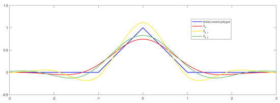
Figure 1. Basic limit functions of $S_8,S_{8\_1},S_{8\_2}.$

4.3. New Subdivision Scheme Deduced from the $C_2$-Scheme

In 2013, Cashman et al. [18] presented C-schemes, which generalized the Lane–Riesenfeld algorithm [2] by using the same operator of a local cubic interpolant to every four adjacent values to define each refining and smoothing stage. In this paper, for simplicity, we call the C-scheme with k smoothing steps the $C_k$-scheme. The symbol of the $C_2$-scheme is:

$$\begin{array}{cc}\hfill a(z)& =\frac{{(1+z)}^6}{32z^3}·\frac{(-1+4z-z^2){(-1+10z-z^2)}^2}{128z^3}\hfill \\ \hfill & =\frac{-(1+z^{12})+18(z+z^{11})-54(z^2+z^{10})-310(z^3+z^9)+225(z^4+z^8)+2340(z^5+z^7)+3756z^6}{4096z^6},\hfill \end{array}$$

$N=12,$

$$(a_0,a_1,a_2,\dots ,a_{12})$$

$$=\frac{1}{4096}(-1,18,-54,-310,225,2340,3756,2340,225,-310,-54,18,-1),$$

$d_{G_a}$ = 5, and $d_{R_a}$ = 3 [18]. From Proposition 1, $k=1,$ one scheme $S_{b_1}$ with $d_{R_{b_1}}=5$ can be deduced from $S_a$.

Using (9) and (8), we have

$$(a_0,a_0^{[1]},a_0^{[2]},a_0^{[3]},a_0^{[4]})=\frac{1}{4096}(-1,6,72,-224,-1920),$$

and

$$\begin{array}{c}\hfill a(z)=\frac{-{(1-z)}^{12}+6{(1-z)}^{10}·z+72{(1-z)}^8·z^2-224{(1-z)}^6·z^3-1920{(1-z)}^4·z^4}{4096z^6}+2.\end{array}$$

By (10) and (11), we obtain $l_1=-\frac{a_0^{[4]}}{2}=\frac{1920}{2·4096}=\frac{15}{64},$ and ${\rho }_1(z)=\frac{15{(1-z)}^4}{64z^2},$ thus

$$\begin{array}{cc}\hfill b_1(z)& =a(z)·(1+{\rho }_1(z))\hfill \\ \hfill & =\frac{{(1+z)}^6}{32z^3}·\frac{(-1+4z-z^2){(-1+10z-z^2)}^2}{128z^3}·\left(\frac{15-60z+154z^2-60z^3+15z^4}{64z^2}\right),\hfill \end{array}$$

which is a new scheme $S_{b_1},$ denoted by $C_{2\_1},$ with $d_{R_{b_1}}=5$ deduced from the $C_2$-scheme with $d_{R_a}=3$. It should be noted that, although $d_{G_{b_1}}=d_{R_{b_1}}=5,$ the new scheme $C_{2\_1}$ is not an interpolatory one. In Figure 2, the basic limit functions of $C_2$ (red), $C_{2\_1}$ (yellow) are illustrated.

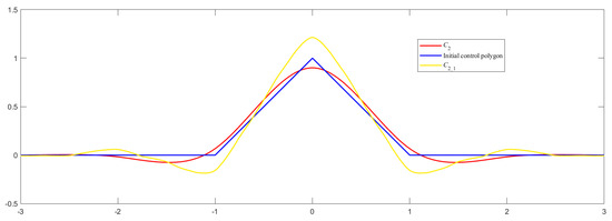
Figure 2. Basic limit functions of $C_2,C_{2\_1}.$

Now, let us consider the examples for even symmetric subdivision schemes.

4.4. Subdivision Scheme Deduced from Uniform Quartic B-Spline Refinement

The symbol of uniform quartic B-spline refinement is

$$a(z)=\frac{{(1+z)}^5}{16z^3},$$

then $N=5,$

$$m(z)=a(z^2)·z=\frac{{(1+z^2)}^5}{16z^5}=\frac{(1+z^{10})+5(z^2+z^8)+10(z^4+z^6)}{16z^5},$$

$$(m_0,m_1,m_2,\dots ,m_{10})=\frac{1}{16}(1,0,5,0,10,0,10,0,5,0,1),$$

$d_{G_a}$ = 4, and $d_{R_a}$ = 1. From Proposition 2, $k=1,$ one scheme $S_{b_1}$ with $d_{R_{b_1}}=3$ can be deduced from $S_a$. Using (20) and (19), we have

$$(m_0,m_0^{[1]},m_0^{[2]},m_0^{[3]},m_0^{[4]})=\frac{1}{16}(1,10,40,80,80),$$

and

$$\begin{array}{c}\hfill a(z^2)·z=m(z)=\frac{{(1-z)}^{10}+10{(1-z)}^8·z+40{(1-z)}^6·z^2+80{(1-z)}^4·z^3+80{(1-z)}^2·z^4}{16z^5}+2.\end{array}$$

Using (3), we have

$$\begin{array}{cc}\hfill b(z^2)·z-2& =a(z^2)·z-2+a(z^2)·z·\rho (z^2)\hfill \\ \hfill & =\frac{{(1-z)}^{10}+10{(1-z)}^8·z+40{(1-z)}^6·z^2+80{(1-z)}^4·z^3+80{(1-z)}^2·z^4}{16z^5}\hfill \\ \hfill & +\frac{{(1-z)}^{10}+10{(1-z)}^8·z+40{(1-z)}^6·z^2+80{(1-z)}^4·z^3+80{(1-z)}^2·z^4+32z^5}{16z^5}·\rho (z^2).\hfill \end{array}$$

At this point, by (23) and (22), we obtain $t_1=-\frac{m_0^{[4]}}{8}=-\frac{5}{8},$ and ${\rho }_1(z^2)=-\frac{5}{8}·\frac{{(1-z^2)}^2}{z^2},$ thus

$$b_1(z)=a(z)·(1+{\rho }_1(z))=\frac{{(1+z)}^5}{16z^3}·\left(1-\frac{5{(1-z)}^2}{8z}\right)=\frac{{(1+z)}^5}{16z^3}·\left(\frac{-5+18z-5z^2}{8z}\right).$$

That is, from the given scheme $S_a$ with $d_{R_a}=1$, we obtain $S_{b_1}$ with $d_{{R_b}_1}=3$, which is precisely the dual 4-point scheme proposed in [6].

4.5. New Subdivision Scheme $S_{7\_1}$ Deduced from Hormann–Sabin’s Family $S_7$

$S_7$ [8] has the symbol

$$a(z)=\frac{{(1+z)}^7}{64z^4}·\frac{-7+22z-7z^2}{8z}=\frac{-7(1+z^9)-27(z+z^8)+168(z^3+z^6)+378(z^4+z^5)}{512z^5}.$$

Here $N=9,$

$$(m_0,m_1,m_2,\dots ,m_{18})=\frac{1}{512}(-7,0,-27,0,0,0,168,0,378,0,378,0,168,0,0,0,-27,0,-7),$$

$d_{G_a}$ = 6, and $d_{R_a}$ = 3. From Proposition 2, $k=1,$ one scheme $S_{b_1}$ with $d_{R_{b_1}}=5$ can be deduced from $S_a$. Using (20), we have

$$(m_0,m_0^{[1]},m_0^{[2]},\dots ,m_0^{[7]})=\frac{1}{512}(-7,-126,-972,-4200,-11088,-18144,-17472,-8064).$$

By (24) and (25), we obtain $t_1=-\frac{m_0^{[7]}}{32}=\frac{63}{128},$ and ${\rho }_1(z)=\frac{63}{128}·\frac{{(1-z)}^4}{z^2},$ thus

$$b_1(z)=a(z)·(1+{\rho }_1(z))=\frac{{(1+z)}^7}{64z^4}·\frac{-7+22z-7z^2}{8z}·\left(\frac{63-252z+506z^2-252z^3+63z^4}{128z^2}\right).$$

That is, from the given scheme $S_a$ with $d_{R_a}=3$, $S_{b_1},$ denoted by $S_{7\_1},$ we obtain $d_{{R_b}_1}=5$.

In Figure 3, the basic limit functions of $S_7$ (red), $S_{7\_1}$ (yellow) are illustrated.

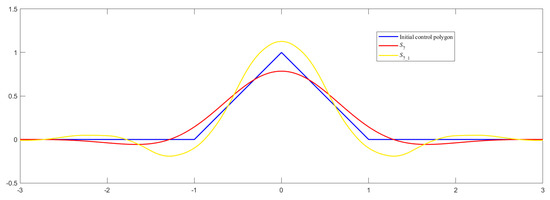
Figure 3. Basic limit functions of $S_7,S_{7\_1}.$

4.6. New Subdivision Scheme Deduced from the $C_3$-Scheme

The symbol of the $C_3$-scheme is

$$a(z)=\frac{{(1+z)}^7·(-1+4z-z^2)·{(-1+10z-z^2)}^3}{65536z^8}.$$

Here, $N=15,$

$$\begin{array}{c}\hfill (m_0,m_1,m_2,\dots ,m_{30})=\frac{1}{65536}(1,0,-27,0,207,0,-13,0,-3519,0,-3051,0,19639,0,52299,\\ \hfill 0,52299,0,19639,0,-3051,0,-3519,0,-13,0,207,0,-27,0,1),\end{array}$$

$d_{G_a}$ = 6, and $d_{R_a}$ = 3 [18]. From Proposition 2, $k=1,$ one scheme $S_{b_1}$ with $d_{R_{b_1}}=5$ can be deduced from $S_a$.

Using (20), we have

$$\begin{array}{c}\hfill (m_0,m_0^{[1]},\dots ,m_0^{[13]})=\frac{1}{65536}(1,30,378,2548,9384,14256,-21920,-128448,\\ \hfill -155520,159488,559104,276480,-483328,-540672).\end{array}$$

By (24) and (25), we obtain $t_1=-\frac{m_0^{[13]}}{32}=\frac{540672}{32·65536}=\frac{33}{128},$ and ${\rho }_1(z^2)=\frac{33}{128}·\frac{{(1-z^2)}^4}{z^4},$ thus

$$\begin{array}{cc}\hfill b_1(z)& =a(z)·(1+{\rho }_1(z))\hfill \\ \hfill & =\frac{{(1+z)}^7·(-1+4z-z^2)·{(-1+10z-z^2)}^3}{65536z^8}·\left(\frac{33-132z+326z^2-132z^3+33z^4}{128z^2}\right).\hfill \end{array}$$

Hence, from the given scheme $S_a$ with $d_{R_a}=3$, $S_{b_1},$ denoted by $C_{3\_1},$ we obtain $d_{{R_b}_1}=5$. In Figure 4, the basic limit functions of $C_3$ (red), $C_{3\_1}$ (yellow) are illustrated.

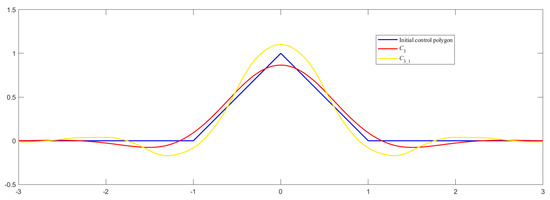
Figure 4. Basic limit functions of $C_3,C_{3\_1}.$

Remark 5. 

If the original scheme $S_a$ is a uniform B-spline refinement, then, using the computational formulas provided in Table 1 and Table 3, it can be verified that the new schemes deduced are exactly the rest of the members of the family of pseudo-splines, which $S_a$ is included in. For example, if $S_a$ is the primal pseudo-spline $S_{a_4^0},$ with $d_{G_a}$ = 7 and $d_{R_a}$ = 1, then we can compute via Table 1 that $S_{b_k}, k=1,2,3,$ are exactly pseudo-splines $S_{a_4^l}, l=1,2,3,$ respectively.

Remark 6. 

Note that $S_8$ in [8] is actually pseudo-spline $S_{a_4^1},$ but $S_{8\_1}$ is not pseudo-spline $S_{a_4^2}.$ Although $S_{8\_1}$ and $S_{a_4^2}$ both have degree-5 polynomial reproduction, the support of $S_{8\_1}$ is wider than $S_{a_4^2}$. This is because $S_{8\_1}$ is obtained from $S_8=S_{a_4^1}$, while $S_{a_4^2}$ is deduced directly from $S_{a_4^0},$ whose support is narrower.

In Table 5, we list comparisons of the reproduction properties of deduced subdivision schemes with the corresponding properties of original subdivision schemes included in this section. Additionally, we illustrate the polynomial reproduction capabilities (red) of $S_{8\_2}$ with 1-step subdivision for Legendre polynomials (blue) from degree 2 to degree 7 from initial points (yellow) in Figure 5.

Table 5. Comparison of the reproduction properties of deduced subdivision schemes with the corresponding properties of original subdivision schemes. (I—interpolatory, A—approximating).

Original Scheme	Primal/Dual	${\mathit{d}}_{{\mathit{G}}_{\mathit{a}}}$	${\mathit{d}}_{{\mathit{R}}_{\mathit{a}}}$	New Scheme Deduced (${\mathit{d}}_{{\mathit{R}}_{\mathit{b}}}$)	I/A
Cubic B-spline	Primal	3	1	4-point scheme (3)	I
$S_8$	Primal	7	3	$S_{8\_1}$ (5); $S_{8\_2}$ (7)	A; A
$C_2$	Primal	5	3	$C_{2\_1}$ (5)	A
Quartic B-spline	Dual	4	1	Dual 4-point scheme (3)	A
$S_7$	Dual	6	3	$S_{7\_1}$ (5)	A
$C_3$	Dual	6	3	$C_{3\_1}$ (5)	A

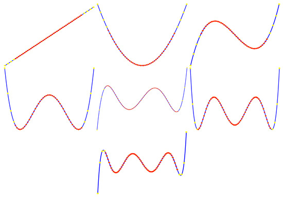
Figure 5. Polynomial reproduction capabilities (red) of $S_{8\_2}$ for Legendre polynomials (blue) from degree 2 to degree 7 with 1-step subdivision from initial points (yellow).

5. Conclusions and Future Work

We have introduced a direct method for constructing subdivision schemes reproducing high-degree polynomials. The method is demonstrated with odd symmetric subdivision and even symmetric subdivision. The advantages of our method are mainly twofold, i.e., the constants of $l_k$ and $t_k$ can be computed rapidly and the form of the generating function of deduced subdivision is determinate. We will consider a similar method for polynomial reproduction of tensor-product and non-tensor-product schemes as our future work.

References

- Dyn, N.; Levin, D.; Gregory, J.A. A 4-point interpolatory subdivision scheme for curve design. Comput. Aided Geom. Des. 1987, 4, 257–268. [Google Scholar] [CrossRef]
- Lane, J.M.; Riesenfeld, R.F. A theoretical development for the computer generation and display of piecewise polynomial surfaces. IEEE Trans. Pattern Anal. Mach. Intell. 1980, 2, 35–46. [Google Scholar] [CrossRef] [PubMed]
- Dyn, N.; Hormann, K.; Sabin, M.A.; Shen, Z. Polynomial reproduction by symmetric subdivision schemes. J. Approx. Theory 2008, 155, 28–42. [Google Scholar] [CrossRef]
- Levin, A. Polynomial generation and quasi-interpolation in stationary non-uniform subdivision. Comput. Aided Geom. Des. 2003, 20, 41–60. [Google Scholar] [CrossRef]
- Conti, C.; Hormann, K. Polynomial reproduction for univariate subdivision schemes of any arity. J. Approx. Theory 2011, 163, 413–437. [Google Scholar] [CrossRef]
- Dyn, N.; Floater, M.S.; Hormann, K. A C2 Four-Point Subdivision Scheme with Fourth Order Accuracy and Its Extensions. In Mathematical Methods for Curves and Surfaces: Tromsø; Nashboro Press: Brentwood, TN, USA, 2005; pp. 145–156. [Google Scholar]
- Choi, S.W.; Lee, B.G.; Lee, Y.J.; Yoon, J. Stationary subdivision schemes reproducing polynomials. Comput. Aided Geom. Des. 2006, 23, 351–360. [Google Scholar] [CrossRef]
- Hormann, K.; Sabin, M.A. A family of subdivision schemes with cubic precision. Comput. Aided Geom. Des. 2008, 25, 41–52. [Google Scholar] [CrossRef]
- Charina, M.; Conti, C. Polynomial reproduction of multivariate scalar subdivision schemes. J. Comput. Appl. Math. 2013, 240, 51–61. [Google Scholar] [CrossRef]
- Deng, C.; Ma, W. Efficient evaluation of subdivision schemes with polynomial reproduction property. J. Comput. Appl. Math. 2016, 294, 403–412. [Google Scholar] [CrossRef]
- Jeong, B.; Yoon, J. Construction of Hermite subdivision schemes reproducing polynomials. J. Math. Anal. Appl. 2017, 451, 565–582. [Google Scholar] [CrossRef]
- Conti, C.; Hüning, S. An algebraic approach to polynomial reproduction of Hermite subdivision schemes. J. Comput. Appl. Math. 2019, 349, 302–315. [Google Scholar] [CrossRef]
- Hüning, S. Polynomial reproduction of Hermite subdivision schemes of any order. Math. Comput. Simul. 2020, 176, 195–205. [Google Scholar] [CrossRef]
- Dong, B.; Shen, Z. Pseudo-splines, wavelets and framelets. Appl. Comput. Harmon. Anal. 2007, 22, 78–104. [Google Scholar] [CrossRef][Green Version]
- Conti, C.; Deng, C.; Hormann, K. Symmetric four-directional bivariate pseudo-spline symbols. Comput. Aided Geom. Des. 2018, 60, 10–17. [Google Scholar] [CrossRef]
- Conti, C.; Romani, L. Algebraic conditions on non-stationary subdivision symbols for exponential polynomial reproduction. J. Comput. Appl. Math. 2011, 236, 543–556. [Google Scholar] [CrossRef]
- Romani, L. From approximating subdivision schemes for exponential splines to high-performance interpolating algorithms. J. Comput. Appl. Math. 2009, 224, 383–396. [Google Scholar] [CrossRef]
- Cashman, T.J.; Hormann, K.; Reif, U. Generalized Lane-Riesenfeld algorithms. Comput. Aided Geom. Des. 2013, 30, 398–409. [Google Scholar] [CrossRef]
Disclaimer/Publisher’s Note: The statements, opinions and data contained in all publications are solely those of the individual author(s) and contributor(s) and not of MDPI and/or the editor(s). MDPI and/or the editor(s) disclaim responsibility for any injury to people or property resulting from any ideas, methods, instructions or products referred to in the content. |
© 2023 by the authors. Licensee MDPI, Basel, Switzerland. This article is an open access article distributed under the terms and conditions of the Creative Commons Attribution (CC BY) license (https://creativecommons.org/licenses/by/4.0/).