Approximate Solutions for a Class of Predator–Prey Systems with Nonstandard Finite Difference Schemes

Abstract

In this paper, we construct new nonstandard finite difference schemes to approximate a set of positive solutions for the predator–prey model, which contains different functional responses. The organization of the denominator of the discrete derivative and nonlocal approximations of nonlinear terms are employed to design the new schemes. The approach results in significant qualitative improvements in how the numerical solution behaves. We establish that the proposed nonstandard finite difference methods are elementary stable and satisfy the positivity requirement. In addition, the instances of applying PESN methods to some predator–prey systems using the Beddington–DeAngelis and Nicholson–Bailey functional responses are provided here. Finally, some numerical comparisons are presented to illustrate our findings. Our results indicate that the proposed methods are very suitable for the symmetric model of predator–prey.

1. Introduction

Symmetry in mathematics often emerges in mathematical models. This concept helps to find the high-quality results for vital problems in a variety of fields. The predator–prey model is one of these problems, which is introduced in full below. The following nonlinear system, which pertains to ordinary differential equations, provides a general model for the predator–prey systems an important phenomena in the biological systems [1,2,3,4]:

$$\begin{array}{cc}\hfill \frac{ds}{dt}& =p\left(s\right)-arf(s,r);s\left(0\right)\ge 0,\hfill \\ \hfill \frac{dr}{dt}& =rf(s,r)-\mu \left(r\right);r\left(0\right)\ge 0,\hfill \end{array}$$

(1)

where s and r stand for the prey and predator population sizes. Here, $p\left(s\right)=s$ indicates the inherent rate of growth in the prey and $\mu \left(r\right)=dr$ the mortality rate of the predator. The transformation rate constant a stands for the assimilation efficiency of the predator, and the function $f(s,r)=sg(s,r)$ is designated as a functional response, indicating the per capita predator feeding rate per unit time. Following [3], it is assumed

$$g(s,r)>0,s{\displaystyle \frac{\partial g}{\partial s}}+g>0,{\displaystyle \frac{\partial g}{\partial r}}<0;(s,r)\in {ℝ}_{+}^2.$$

(2)

System (1) has been simulated and solved by many numerical methods, those methods are nonstandard finite difference (NSFD) [3,5,6,7,8,9,10,11,12,13,14,15,16,17,18,19,20] and generalized finite difference method (GFDM) [21,22,23].

In this paper, we focus on constructing the new NSFD methods based on whether the numerical solution of (1) is positive and elementary stable with appropriate choices of the model parameters [4,24,25,26,27,28,29,30,31,32,33]. In fact, the main motivation of this paper is to solve predator–prey systems with simple and low computational cost methods while preserving qualitative characteristics such as positivity and boundedness. These nonstandard methods are more effective than standard methods, such as the RK4 method, and standard ready-made MATLAB codes, such as ODE45, to preserve the same qualitative characteristics and having milder oscillations. Moreover, the implementation of these methods with large steps also provides a relatively good solution.

The rest of the paper is structured as follows. In Section 2, we present some preliminaries. Section 3 provides the new schemes. In Section 4, the positivity property of the new schemes is presented. In Section 5, the elementary stability of the proposed schemes is analyzed. Section 6 is devoted to the results of the proposed schemes, the fourth-order Runge–Kutta (RK4) method, and the existing NSFD method in [3]. Finally, Section 7 wraps up the paper with some conclusions.

2. Preliminaries

System (1) has two equilibria as:

(i)

The trivial equilibrium $(s_0,r_0)=(0,0)$;

(ii)

An interior equilibrium $(s^{*},r^{*})$ satisfying $s^{*}g(s^{*},r^{*})=d$ and $s^{*}=ad{r}^{*}$;

where $(0,0)$ is always linearly unstable and the interior equilibrium $(s^{*},r^{*})$ is linearly stable if

$$D(s^{*},r^{*})=s^{*}\frac{\partial g}{\partial r}+ad{s}^{*}\frac{\partial g}{\partial s}+adg>0$$

and

$$T(s^{*},r^{*})=s^{*}{r}^{*}\frac{\partial g}{\partial r}-a{s}^{*}{r}^{*}\frac{\partial g}{\partial s}<0$$

are satisfied simultaneously, see [3,34,35] for more details.

System (1) is a first-order system of ordinary differential equations (ODEs). General first-order system ODEs, can be written as follows:

$$\frac{d}{dt}V\left(t\right)=F\left(V\left(t\right)\right),(t\ge 0),V\left(0\right)=V_0,$$

(3)

where V can be regarded as a single function or as a vector of functions of length k mapping $[t_0,T)\to {\mathcal{C}}^k,$ and the corresponding F is a single function or a vector of functions of length k mapping $([t_0,T),{\mathcal{C}}^k)\to ([t_0,T),{\mathcal{C}}^k)$. If we define $t_n=t_0+nh$, where $h>0$ is step-size and

$$V_n\approx V\left(t_n\right),$$

(4)

then the discretized version of (3) becomes

$${\mathcal{D}}_h{V}_n={\mathcal{F}}_n(F,V_n),$$

(5)

where ${\mathcal{D}}_h{V}_n$ stands for the discretized model of $\frac{d}{dt}V\left(t\right)$ and ${\mathcal{F}}_n(F,V_n)$ approximates $F\left(V\left(t_n\right)\right)$ at time $t_n$.

The definition of the nonstandard one-step finite difference method rests on Anguelov and Lubuma [34].

Definition 1.

A discrete version of (1) is called the nonstandard method provided that one of the conditions below is satisfied:

(i) 

In the discrete derivatives of $\frac{ds}{dt}$ and $\frac{dr}{dt}$ a non-negative function substitutes the step size h, $\phi \left(h\right)$ such that

$$\phi \left(h\right)=h+O\left(h^2\right)as0<h\to 0;$$

(6)

(ii) 

Nonlinear terms in the right hand side of (1) are approximated in a nonlocal way, that is to say, by an appropriate function of some points in the mesh.

For instance:

$$\begin{array}{cc}\hfill V& \approx 2V_n-V_{n+1},\hfill \\ \hfill V^2& \approx V_n\ast V_{n+1},\hfill \\ \hfill V^3& \approx \alpha V_n^2\ast V_{n+1}+(1-\alpha )V_n\ast V_{n+1}\ast V_{n-1}.\hfill \end{array}$$

3. Development of New NSFD Schemes

Using the strategy of the nonstandard discretization methods [27,29], we propose a family of positive and elementary stable nonstandard (PESN) schemes for system (1) of the form:

$$\begin{array}{cc}\hfill {\displaystyle \frac{s_{k+1}-s_k}{\phi \left(h\right)}}& =(\delta s_k+\eta s_{k+1})-ag(s_k,r_k)(\gamma s_{k+1}{r}_k+\theta s_k{r}_{k+1}),\hfill \\ \hfill {\displaystyle \frac{r_{k+1}-r_k}{\phi \left(h\right)}}& =g(s_k,r_k)(\gamma s_{k+1}{r}_k+\theta s_k{r}_k)-d(\delta r_{k+1}+\eta r_k)\hfill \end{array}$$

(7)

with $\delta +\eta =1,\gamma +\theta =1$ and

$$\phi \left(h\right)=\frac{\varphi \left(hq\right)}{q}$$

for $0<\varphi \left(hq\right)<1.$

By selecting different parameters for the above system, we examined the constructed methods and gave two examples. It is worth noting that the following methods, unlike the standard methods known as RK4 and RK2, retain the positive property, one of the most important properties of the predator–prey model, and have better speed and convergence to equilibrium points. Further, these methods have less fluctuations and better convergence than other nonstandard methods, such as the suggested method in [7].

3.1. Scheme 1

After taking the values of $\delta =2,\eta =-1,\gamma =1,\theta =0$ into the (7), the discrete method is obtained as follows:

$$\begin{array}{cc}\hfill s_{k+1}& ={\displaystyle \frac{1+2\phi \left(h\right)}{1+\phi \left(h\right)(1+a{r}_{k}g(s_k,r_k))}}{s}_k,\hfill \\ \hfill r_{k+1}& ={\displaystyle \frac{1+\phi \left(h\right)(d+s_{k+1}g(s_k,r_k))}{1+2d\phi \left(h\right)}}{r}_k.\hfill \end{array}$$

(8)

3.2. Scheme 2

It is produced by taking $\delta =1,\eta =0,\gamma =2,\theta =-1,q=1,\varphi \left(h\right)=h$, which results in

$$\begin{array}{cc}\hfill s_{k+1}& ={\displaystyle \frac{1+h+ah{r}_{k}g(s_k,r_k)}{1+2a{r}_{k}hg(s_k,r_k)}}{s}_k,\hfill \\ \hfill r_{k+1}& ={\displaystyle \frac{1+2h{s}_{k+1}g(s_k,r_k)}{1+hd+h{s}_{k}g(s_k,r_k)}}{r}_k.\hfill \end{array}$$

(9)

4. Positivity

Under this heading, we examine positivity as a property of the method devised in the previous section. The property suggests that the component-wise non-negativity of the initial vector is preserved in time for the solution. Mention should be made of the fact that positivity preserving of a numerical method is important when it is employed to solve differential models associated with population biology, for these state variables stand for subpopulations that never take negative values. There are many NSFD schemes in the literature.

Definition 2.

A discrete finite-difference scheme is called positive if the corresponding solution of this scheme is non-negative for any $h>0$, and $r_0\in {ℝ}_{+}^n$, i.e., for all $k\in \mathbb{N}$, $r_k\in {ℝ}_{+}^n$.

The new schemes preserve the positivity property as expressed in the following theorem:

Theorem 1.

The schemes (8) and (9) for solving system (1) are positivity.

Proof. 

It can be easily concluded that schemes (8) and (9) are unconditionally positive (for any $h>0$ ) as the constants $a,d>0$. □

5. Elementary Stability

The construction of difference schemes, preserving the local stability of the equilibrium points, is of great importance in the numerical solution of ODEs. The difference schemes with this stability property are named elementary stable schemes [6,26,34,36].

Definition 3.

The finite difference method is regarded as elementary stable, provided that for any value of the step size h, its only equilibrium points E can be of the original differential system and the linear stability properties of each E are akin to both the differential system and the discrete method.

This section is devoted to presenting the main result of this paper. In order to prove this result, the lemma below is required, which can be seen in [4,7].

Lemma 1.

For the quadratic equation ${\lambda }^2+\Lambda \lambda +{\rm Y}=0$ by applying the famous Jury condition [4,11], both roots satisfy $|{\lambda }_i|<1$, $i=1,2$ if the conditions below are met:

(i) 

$1+\Lambda +{\rm Y}>0$;

(ii) 

$1-\Lambda +{\rm Y}>0$;

(iii) 

${\rm Y}<1$.

Theorem 2.

The schemes in (8) and (9) are elementary stables.

Proof. 

The Jacobian J of the scheme (8) has the form $J(s_k,r_k)={\left[j_{mn}(s_k,r_k)\right]}_{2\times 2}$, for $m,n=1,2$, where

$$\begin{array}{cc}\hfill j_{11}(s_k,r_k)& =\frac{1+2\phi \left(h\right)}{1+\phi \left(h\right)(1+a{r}_{k}g(s_k,r_k))}-{\displaystyle \frac{a{r}_k\phi \left(h\right)\frac{\partial g}{\partial s}(s_k,r_k)\left(1+2\phi \left(h\right)\right)}{{[1+\phi \left(h\right)(1+a{r}_{k}g(s_k,r_k))]}^2}}{s}_k,\hfill \\ \hfill j_{12}(s_k,r_k)& =-{\displaystyle \frac{a\phi \left(h\right)\left(g(s_k,r_k)+r_k\frac{\partial g}{\partial r}(s_k,r_k)\right)\left(1+2\phi \left(h\right)\right)}{{[1+\phi \left(h\right)(1+a{r}_{k}g(s_k,r_k))]}^2}}{s}_k,\hfill \\ \hfill j_{21}(s_k,r_k)& ={\displaystyle \frac{\phi \left(h\right)\left(g(s_k,r_k)j_{11}(s_k,r_k)+s_{k+1}\frac{\partial g}{\partial s}(s_k,r_k)\right)}{1+2d\phi \left(h\right)}}{r}_k,\hfill \\ \hfill j_{22}(s_k,r_k)& ={\displaystyle \frac{1+\phi \left(h\right)\left(d+s_{k+1}g(s_k,r_k)+j_{12}(s_k,r_k)g(s_k,r_k)r_k+s_{k+1}{r}_k\frac{\partial g}{\partial r}(s_k,r_k)\right)}{1+2d\phi \left(h\right)}}.\hfill \end{array}$$

Substituting $(s_0,r_0)=(0,0)$, we obtain

$$\begin{array}{c}\hfill J(0,0)=\left(\begin{array}{cc}{\displaystyle \frac{1+2\phi \left(h\right)}{1+\phi \left(h\right)}}& 0\\ 0& {\displaystyle \frac{1+d\phi \left(h\right)}{1+2d\phi \left(h\right)}}\end{array}\right).\end{array}$$

The eigenvalues of the matrix are

$${\lambda }_1={\displaystyle \frac{1+2\phi \left(h\right)}{1+\phi \left(h\right)}}\mathrm{and}{\lambda }_2={\displaystyle \frac{1+d\phi \left(h\right)}{1+2d\phi \left(h\right)}}.$$

Since $|{\lambda }_1|>1$ the equilibrium point $(0,0)$ is always unstable. Further, for the equilibrium $(s^{*},r^{*})$, we derive:

$$\begin{array}{cc}\hfill J(s^{*},r^{*})=& \left(\begin{array}{cc}{u}_1& u_2\\ u_3& u_4\end{array}\right),\hfill \end{array}$$

where

$$\begin{array}{cc}\hfill u_1& =1-{\displaystyle \frac{a\phi \left(h\right)s^{*}{r}^{*}\frac{\partial g}{\partial s}(s^{*},r^{*})}{1+2\phi \left(h\right)}},\hfill \\ \hfill u_2& =-{\displaystyle \frac{a\phi \left(h\right)\left(d+s^{*}{r}^{*}\frac{\partial g}{\partial r}(s^{*},r^{*})\right)}{1+2\phi \left(h\right)}},\hfill \\ \hfill u_3& ={\displaystyle \frac{r^{*}\phi \left(h\right)\left(g(s^{*},r^{*})+s^{*}\frac{\partial g}{\partial s}(s^{*},r^{*})\right)}{1+2d\phi \left(h\right)}}-{\displaystyle \frac{{\phi }^2\left(h\right)s^{*}{r}^{*}\frac{\partial g}{\partial s}(s^{*},r^{*})}{(1+2\phi (h\left)\right)(1+2d\phi (h\left)\right)}},\hfill \\ \hfill u_4& =1+{\displaystyle \frac{\phi \left(h\right)s^{*}{r}^{*}\frac{\partial g}{\partial r}(s^{*},r^{*})}{1+2d\phi \left(h\right)}}-{\displaystyle \frac{2{\phi }^2\left(h\right)\left(d+s^{*}{r}^{*}\frac{\partial g}{\partial r}(s^{*},r^{*})\right)}{(1+2\phi (h\left)\right)(1+2d\phi (h\left)\right)}},\hfill \end{array}$$

eigenvalues of $J(s^{*},r^{*})$ are roots of the quadratic equation ${\lambda }^2-\Lambda \lambda +{\rm Y}=0$, where

$$\begin{array}{cc}\hfill \Lambda & =u_1+u_4\hfill \\ \hfill & =2-{\displaystyle \frac{a{s}^{*}{r}^{*}\phi \left(h\right)\frac{\partial g}{\partial s}(s^{*},r^{*})}{1+2\phi \left(h\right)}}+\frac{s^{*}{r}^{*}\phi \left(h\right)\frac{\partial g}{\partial r}(s^{*},r^{*})}{1+2d\phi \left(h\right)}-\frac{{\phi }^2\left(h\right)\left(d+s^{*}{r}^{*}\frac{\partial g}{\partial r}(s^{*},r^{*})\right)}{(1+2\phi (h\left)\right)(1+2d\phi (h\left)\right)},\hfill \\ \hfill {\rm Y}& =u_1{u}_4-u_2{u}_3\hfill \\ \hfill & =1+\frac{\phi \left(h\right)}{(1+2\phi (h\left)\right)(1+2d\phi (h\left)\right)}\left[T(s^{*},r^{*})+s^{*}{r}^{*}\phi \left(h\right)\left(2\frac{\partial g}{\partial r}(s^{*},r^{*})-ad\frac{\partial g}{\partial s}(s^{*},r^{*})\right)\right].\hfill \end{array}$$

The equilibrium $(s^{*},r^{*})$ is stable provided that all conditions of Lemma 1 are true. It is unstable if at least one of the conditions is not met. Assume that $(s^{*},r^{*})$ is stable equilibrium of system (1); therefore, since $D(s^{*},r^{*})>0$ and $T(s^{*},r^{*})<0$ then

$$1-\Lambda +{\rm Y}={\displaystyle \frac{r^{*}}{A}}\phi {\left(h\right)}^{2}D(s^{*},r^{*})>0,$$

where $A=(1+2\phi (h\left)\right)(1+2d\phi (h)$. Note that $\Lambda =\Lambda \left(\phi \right(h\left)\right)$ and ${\rm Y}={\rm Y}\left(\phi \right(h\left)\right)$ are continuous functions of $\phi \left(h\right)$ for $\phi \left(h\right)>0.$ Moreover, $\Lambda \left(0\right)=2$ and ${\rm Y}\left(0\right)=1$, which imply that we have constants $Z_{(s^{*},r^{*})}>0$ such that $1+\Lambda \left(\phi \right(h\left)\right)+{\rm Y}\left(\phi \right(h\left)\right)>0$ for all $0<\phi \left(h\right)<Z_{(s^{*},r^{*})}$. Further, we have

$$\begin{array}{cc}\hfill 1+\Lambda +{\rm Y}& ={\displaystyle \frac{1}{A}}[{\phi }^2\left(h\right)\left(-5ad{s}^{*}{r}^{*}{\displaystyle \frac{\partial g}{\partial s}}+3s^{*}{r}^{*}{\displaystyle \frac{\partial g}{\partial r}}+15d\right)\hfill \\ \hfill & +\phi \left(h\right)\left(-2a{s}^{*}{r}^{*}{\displaystyle \frac{\partial g}{\partial s}}+2s^{*}{r}^{*}{\displaystyle \frac{\partial g}{\partial r}}+8d+8\right)+4]\hfill \end{array}$$

and we want to have a specific $Z_{(s^{*},r^{*})}$ such that $Z_{(s^{*},r^{*})}\le 1/q$. By some calculations, the condition $1+\Lambda +{\rm Y}>0$ is equivalent to

$$M{\phi }^2\left(h\right)+N\phi \left(h\right)+4>0,$$

(10)

where

$$M=3r^{*}T(s^{*},r^{*})-8ad{s}^{*}{r}^{*}{\displaystyle \frac{\partial g}{\partial s}}(s^{*},r^{*})+12d\mathrm{and}N=2D(s^{*},r^{*})+8d+8.$$

Therefore, following [3], the constant $Z_{(s^{*},r^{*})}$ can be selected as follows:

$$Z_{(s^{*},r^{*})}=\left\{\begin{array}{cc}{\displaystyle \frac{2}{\sqrt{\left|M\right|}}},\hfill & \mathrm{for}N=0;\hfill \\ {\displaystyle \frac{4}{\left|N\right|}},\hfill & \mathrm{for}M=0;\hfill \\ min\left({\displaystyle \frac{\left|N\right|}{\left|M\right|}},{\displaystyle \frac{2}{\left|N\right|}}\right),\hfill & \mathrm{otherwise}.\hfill \end{array}\right.$$

(11)

The condition ${\rm Y}<1$ is equivalent to

$$\begin{array}{c}\hfill T(s^{*},r^{*})+s^{*}{r}^{*}\phi \left(h\right)\left(2{\displaystyle \frac{\partial g}{\partial s}}(s^{*},r^{*})-ad{\displaystyle \frac{\partial g}{\partial s}}(s^{*},r^{*})\right)<0,\end{array}$$

(12)

the inequality (12) is true when $\phi \left(h\right)<Z_{(s^{*},r^{*})}^{*}$ with

$$Z_{(s^{*},r^{*})}^{*}={\displaystyle \frac{\left|T\right(s^{*},r^{*}\left)\right|}{\left|2s^{*}{r}^{*}{\displaystyle \frac{\partial g}{\partial s}}(s^{*},r^{*})-ad{s}^{*}{r}^{*}{\displaystyle \frac{\partial g}{\partial s}}(s^{*},r^{*})\right|}}.$$

(13)

From (11) and (13), if $q>max\left({\displaystyle \frac{1}{Z_{(s^{*},r^{*})}}},{\displaystyle \frac{1}{Z_{(s^{*},r^{*})}^{*}}}\right)$, then following Lemma 1, $E^{*}$ is stable.

The results ensure the dynamical consistency between system (1) and the numerical scheme (8) around all equilibria. The proposed scheme is, therefore, elementary stable.

In a similar way, the equilibrium points of (9) correspond to those of the equilibria of the initial system. The Jacobian J of the scheme (9) has the form $J(s_k,r_k)={\left[j_{mn}(s_k,r_k)\right]}_{2\times 2}$, where

$$\begin{array}{cc}\hfill j_{11}(s_k,r_k)& =\frac{1+h+ah{r}_{k}g(s_k,r_k)+ah{s}_k{r}_k{\displaystyle \frac{\partial g}{\partial s}}(s_k,r_k)}{1+2ah{r}_{k}g(s_k,r_k)}\hfill \\ \hfill & -{\displaystyle \frac{2ah{r}_k{\displaystyle \frac{\partial g}{\partial s}}(s_k,r_k)\left(1+h+ah{r}_{k}g(s_k,r_k)\right)}{{[1+2ah{r}_{k}g(s_k,r_k)]}^2}}{s}_k,\hfill \\ \hfill j_{12}(s_k,r_k)& ={\displaystyle \frac{ah{s}_k\left(g(s_k,r_k)+r_k{\displaystyle \frac{\partial g}{\partial r}}(s_k,r_k)\right)}{1+2ah{r}_{k}g(s_k,r_k)}}\hfill \\ \hfill & -{\displaystyle \frac{2ah\left(g(s_k,r_k)+r_k{\displaystyle \frac{\partial g}{\partial r}}(s_k,r_k)\right)\left(1+h+ah{r}_{k}g(s_k,r_k)\right)}{{[1+2ah{r}_{k}g(s_k,r_k)]}^2}}{s}_k,\hfill \end{array}$$

$$\begin{array}{cc}\hfill j_{21}(s_k,r_k)& ={\displaystyle \frac{2h{r}_k\left(g(s_k,r_k)j_{11}(s_k,r_k)+s_{k+1}{\displaystyle \frac{\partial g}{\partial s}}(s_k,r_k)\right)}{1+hd+h{s}_{k}g(s_k,r_k)}}\hfill \\ \hfill & -{\displaystyle \frac{h\left(g(s_k,r_k)+s_k{\displaystyle \frac{\partial g}{\partial s}}(s_k,r_k)\right)(1+2h{s}_{k+1}g(s_k,r_k))r_k}{{[1+hd+h{s}_{k}g(s_k,r_k)]}^2}},\hfill \end{array}$$

$$\begin{array}{cc}\hfill j_{22}(s_k,r_k)& ={\displaystyle \frac{1+2h\left(s_{k+1}g(s_k,r_k)+j_{12}(s_k,r_k)g(s_k,r_k)r_k+s_{k+1}{r}_k{\displaystyle \frac{\partial g}{\partial r}}(s_k,r_k)\right)}{1+hd+h{s}_{k}g(s_k,r_k)}}\hfill \\ \hfill & -{\displaystyle \frac{\left(h{s}_k{\displaystyle \frac{\partial g}{\partial r}}(s_k,r_k)\right)(1+2h{s}_{k+1}g(s_k,r_k))}{{[1+hd+h{s}_{k}g(s_k,r_k)]}^2}}{r}_k.\hfill \end{array}$$

Substituting $(s_0,r_0)=(0,0)$ in $J(s_k,r_k)$ we derive

$$\begin{array}{c}\hfill J(0,0)=\left(\begin{array}{cc}1+h& 0\\ 0& {\displaystyle \frac{1}{1+hd}}\end{array}\right)\end{array}$$

and its eigenvalues are

$${\lambda }_1=1+h\mathrm{and}{\lambda }_2={\displaystyle \frac{1}{1+hd}}.$$

Since $|{\lambda }_1|>1$ the equilibrium point $(0,0)$ is always unstable. Further, for the equilibrium $(s^{*},r^{*})$, we derive:

$$J(s^{*},r^{*})=\left(\begin{array}{cc}{u}_1& u_2\\ u_3& u_4\end{array}\right),$$

where

$$\begin{array}{cc}\hfill u_1& =1-{\displaystyle \frac{ah{s}^{*}{r}^{*}\frac{\partial g}{\partial s}(s^{*},r^{*})}{1+2h}},\hfill \\ \hfill u_2& =-{\displaystyle \frac{ah\left(d+s^{*}{r}^{*}\frac{\partial g}{\partial r}(s^{*},r^{*})\right)}{1+2h}},\hfill \\ \hfill u_3& ={\displaystyle \frac{h{r}^{*}\left(g(s^{*},r^{*})+s^{*}\frac{\partial g}{\partial s}(s^{*},r^{*})\right)}{1+2hd}}-{\displaystyle \frac{2h^2{s}^{*}{r}^{*}\frac{\partial g}{\partial s}(s^{*},r^{*})}{(1+2h)(1+2hd)}},\hfill \\ \hfill u_4& =1+{\displaystyle \frac{h{s}^{*}{r}^{*}\frac{\partial g}{\partial r}(s^{*},r^{*})}{1+2hd}}-{\displaystyle \frac{2h^2\left(d+s^{*}{r}^{*}\frac{\partial g}{\partial r}(s^{*},r^{*})\right)}{(1+2h)(1+2hd)}},\hfill \end{array}$$

eigenvalues of $J(s^{*},r^{*})$ are roots of the quadratic equation ${\lambda }^2-\Lambda \lambda +{\rm Y}=0$, where

$$\begin{array}{cc}\hfill \Lambda & =2-{\displaystyle \frac{ah{s}^{*}{r}^{*}{\displaystyle \frac{\partial g}{\partial s}}(s^{*},r^{*})}{1+2h}}+{\displaystyle \frac{h{s}^{*}{r}^{*}{\displaystyle \frac{\partial g}{\partial r}}(s^{*},r^{*})}{1+2hd}}-{\displaystyle \frac{2h^2\left(d+s^{*}{r}^{*}{\displaystyle \frac{\partial g}{\partial r}}(s^{*},r^{*})\right)}{(1+2h)(1+2hd)}},\hfill \\ \hfill {\rm Y}& =1+{\displaystyle \frac{h}{(1+2h)(1+2hd)}}\left[T(s^{*},r^{*})+2h{r}^{*}{s}^{*}{\displaystyle \frac{\partial g}{\partial r}}(s^{*},r^{*})-hrD(s^{*},r^{*})\right].\hfill \end{array}$$

Assume that $(s^{*},r^{*})$ is a stable equilibrium of system (1); therefore, since $D(s^{*},r^{*})>0$ and $T(s^{*},r^{*})<0$, then it is clear that

$$\begin{array}{cc}\hfill {\rm Y}& <1,\hfill \\ \hfill 1-\Lambda +{\rm Y}& ={\displaystyle \frac{1}{(1+2h)(1+2hd)}}\left[h^2{r}^{*}D(s^{*},r^{*})\right]>0\hfill \end{array}$$

and we also have

$$\begin{array}{cc}\hfill 1+\Lambda +{\rm Y}& =h^2\left[-3ad{s}^{*}{r}^{*}{\displaystyle \frac{\partial g}{\partial s}}(s^{*},r^{*})+s^{*}{r}^{*}{\displaystyle \frac{\partial g}{\partial r}}(s^{*},r^{*})+13d\right]\hfill \\ \hfill & +h\left[-2a{s}^{*}{r}^{*}{\displaystyle \frac{\partial g}{\partial s}}(s^{*},r^{*})+2s^{*}{r}^{*}{\displaystyle \frac{\partial g}{\partial r}}(s^{*},r^{*})+8d+8\right]+4.\hfill \end{array}$$

We may assume that the inequality $1+\Lambda +{\rm Y}>0$ of the Lemma 1 does not have any formal proof; however, the numerical results in the Math Toolbox software of MATLAB for all step sizes $h>0$ show that the equilibrium point $E^{*}$ is stable. The results can therefore guarantee the dynamic consistency between system (1) and numerical scheme (9) at all equilibria. The corollary is that the scheme is unconditionally elementary stable. □

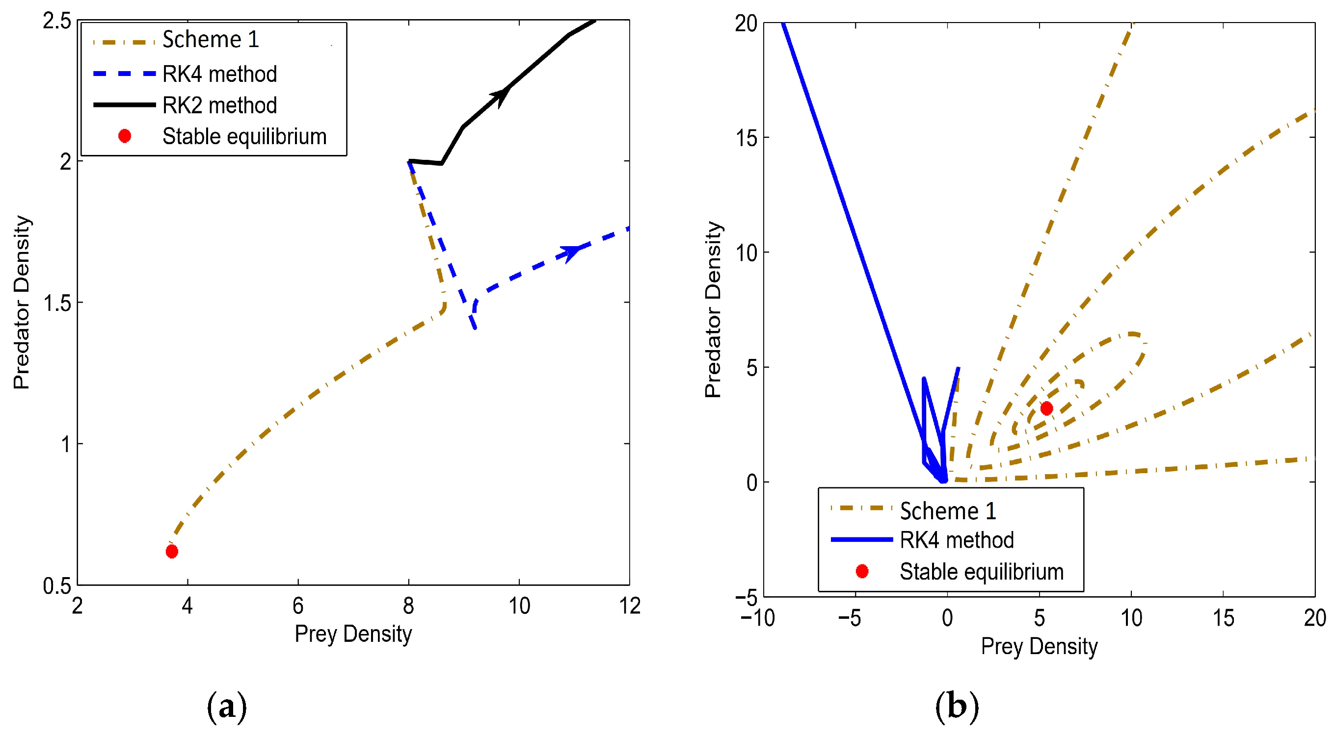
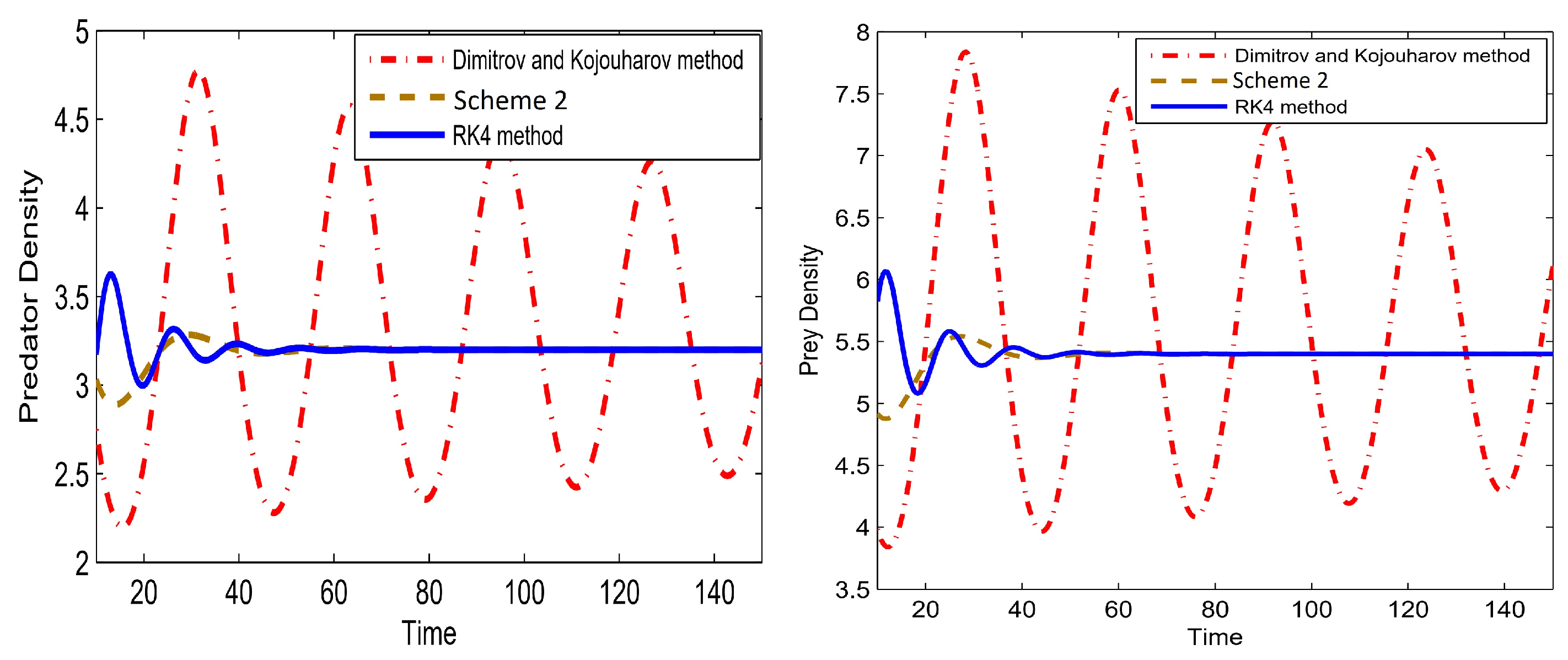
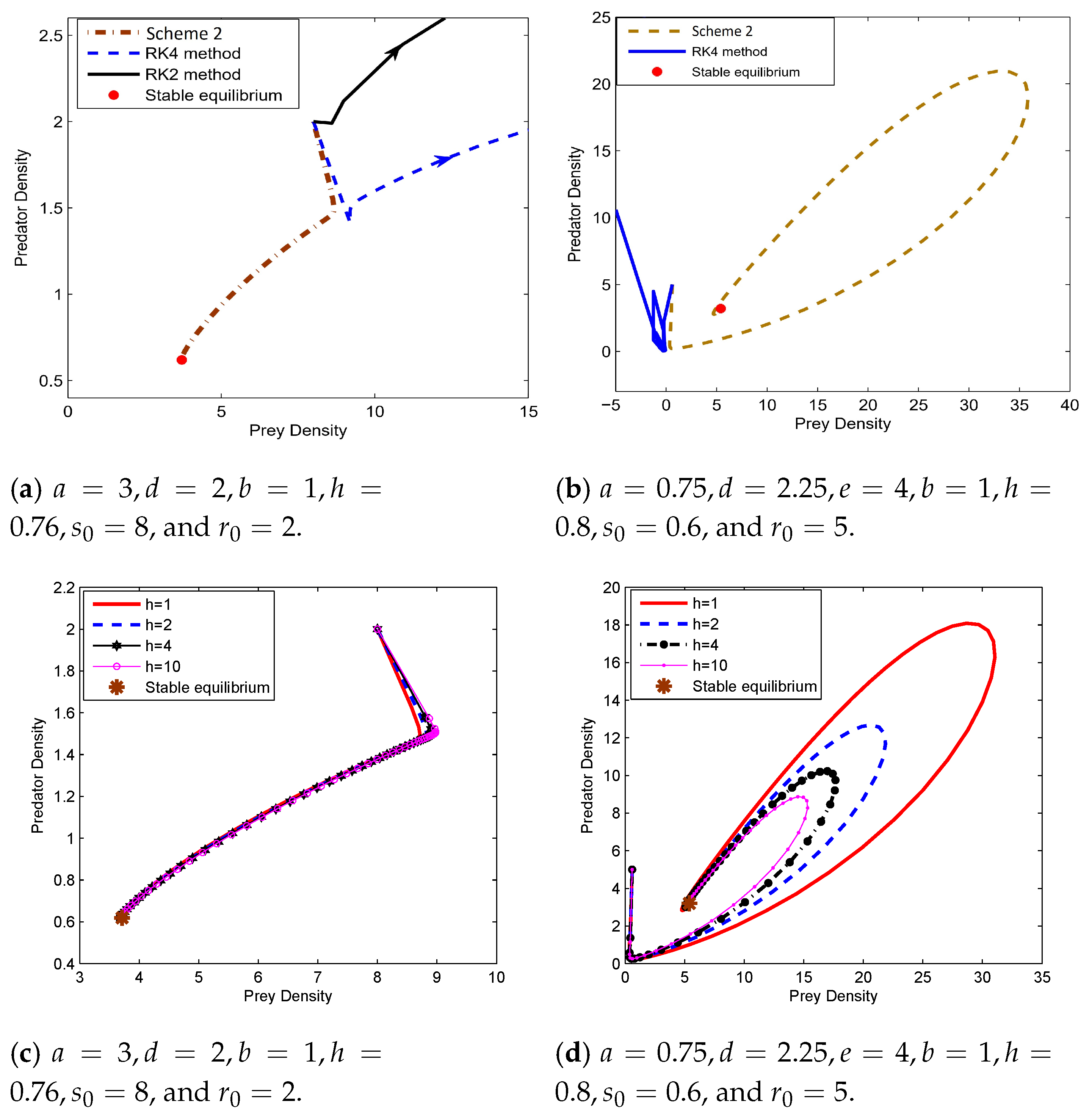
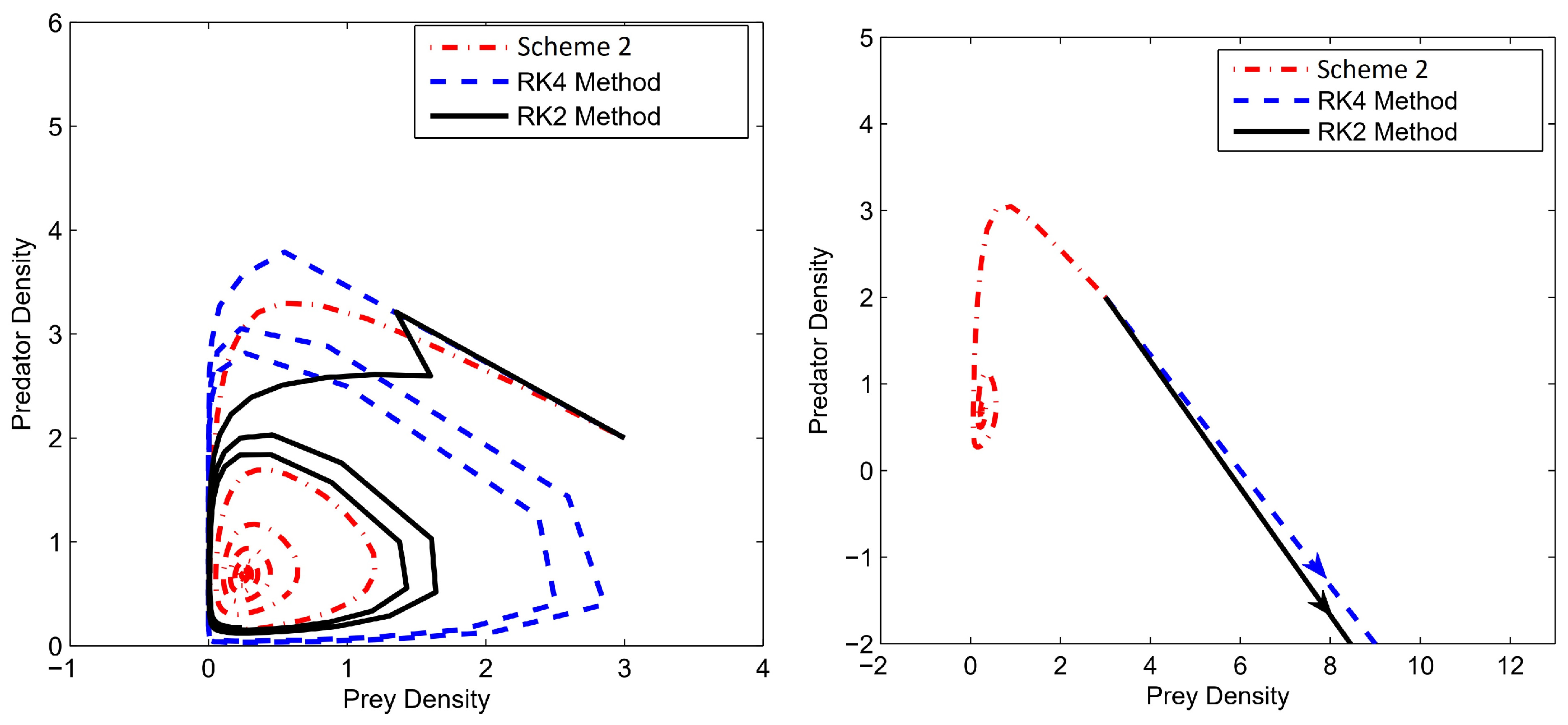
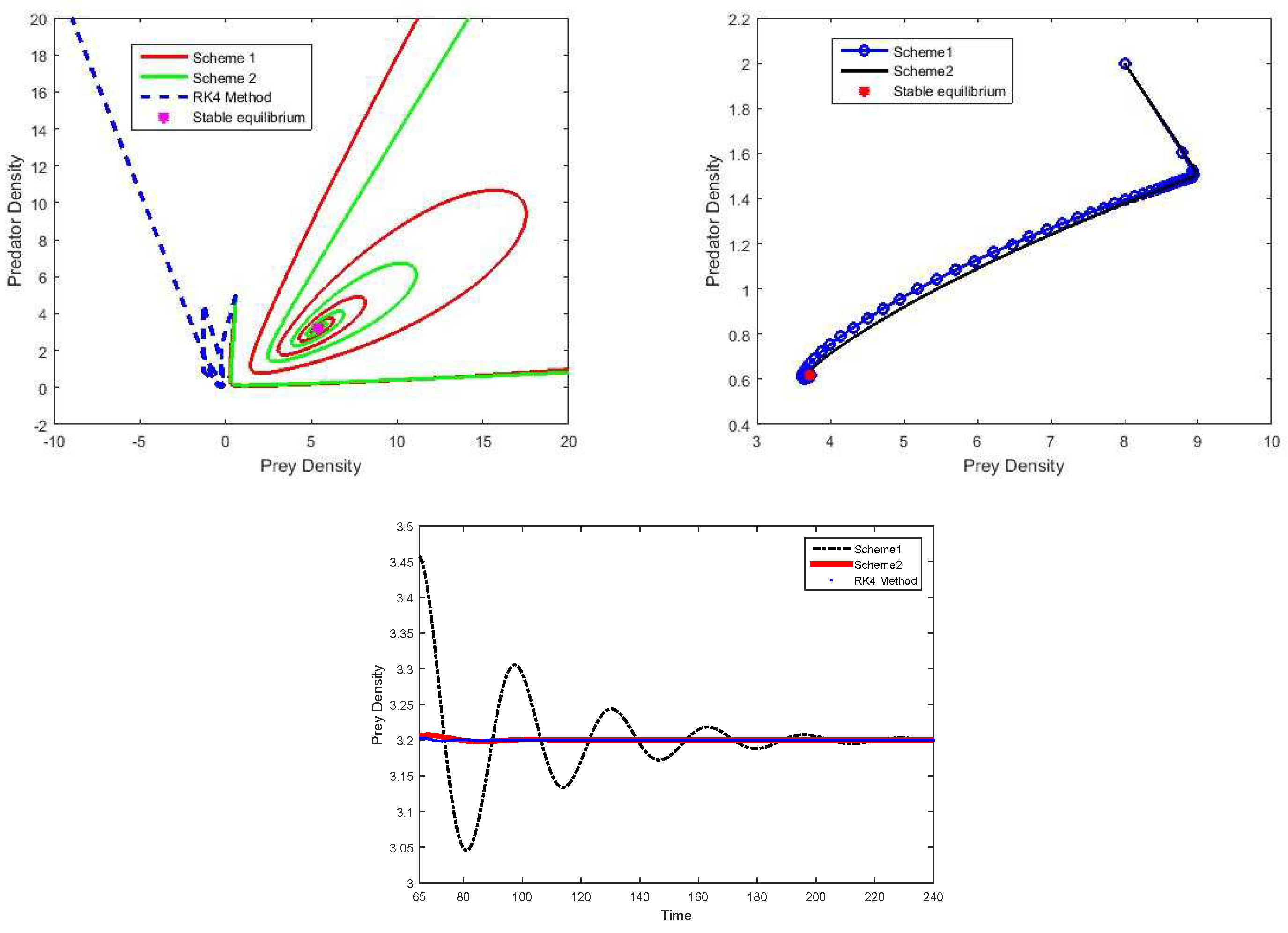
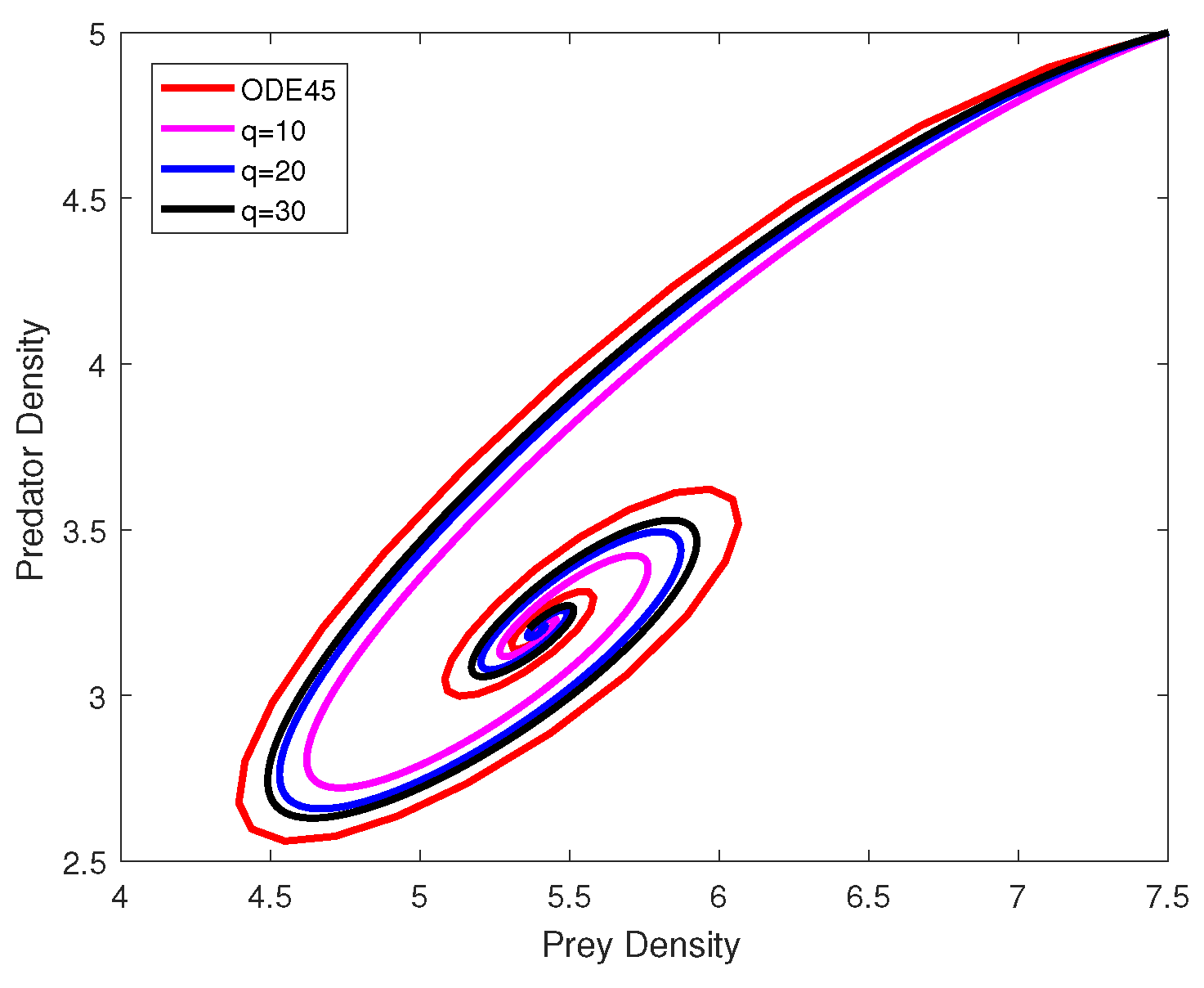
6. Numerical Results

In order to showcase the merits of the proposed PESN finite difference method, we examine the predator–prey system with the Beddington–DeAngelis functional response, $f(s,r)={\displaystyle \frac{es}{b+s+r}}$, and the Nicholson–Bailey functional response $f(s,r)=s{e}^{-br}$ [3,5,6,7]. Numerical approximations of system (1) for the new PESN method (8) and proposed PESN method in [3] with $\phi \left(h\right)=\frac{1-e^{-hq}}{q}$ and classical fourth-order Runge–Kutta (RK4) method are shown in Figure 1. A good agreement has been obtained for scheme 1 and RK4. Further, we see that the new method has the advantage over scheme [3] on achieving a good accuracy. This indicates the axial symmetry trajectory of the system.

Figure 1. Comparing the numerical results of scheme 1 and method [3] with RK4 approximations with $a=0.75, d=2.25, e=4, b=1, h=0.4, s_0=7.5$, and $r_0=5$.

The numerical results for scheme 1 with the Nicholson–Bailey functional response for $a=3, d=2$ and $b=1$ leads to $E^{*}=(3.7144,0.6191)$ and $q>0.62$ are shown in Figure 2a. In this figure, we show that scheme 1 preserves the stability of equilibrium $E^{*}$, while the RK4 and second-order Runge–Kutta (RK2) approximations diverge. For the Beddington–DeAngelis functional response with $a=0.75$, $d=2.25$, $e=4$, and $b=1$ leads to $E^{*}=(27/5,16/5)$ and $q>1.25$; the numerical results are given in Figure 2b. As we can see, scheme 1 is positive and elementary stable while the RK4 method produced a negative value and diverges.

Figure 2. Numerical approximations of system (1) with Nicholson–Bailey functional response (a) $a=3, d=2, b=1, s_0=8$, and $r_0=2$ and Beddington–DeAngelis functional response (b) $a=0.75, d=2.25, e=4, b=1, s_0=0.6$, and $r_0=5$.

Equation (9) for solving Equation (1) with the same parameters used in the previous subsection. As it can be seen in Figure 3, a good agreement has been obtained for the new scheme and RK4 with step size $h=0.4$. While the Dimitrov and Kojouharov method has more oscillations, by comparing the methods, it can be seen that the new method has relatively better accuracy than the Dimitrov and Kojouharov method.

Figure 3. Comparing the numerical results obtained by scheme 2 and method [3] introduced by Dobromir T. Dimitrov and Hristo V. Kojouharov with RK4 approximations with $a=0.75, d=2.25, e=4, b=1, h=0.4, s_0=7.5$, and $r_0=5$.

Figure 4a shows that scheme 2 preserves the stability of the interior equilibrium, whereas the RK2 and RK4 approximations diverge. In Figure 4b, we compare the approximation of the solution obtained by the new method and RK4. In this case, we can see that the RK4 approximations evolve away from the equilibrium point and produce the negative values whereas our scheme preserves the positivity of the solutions and the stability of the equilibrium point. Further, in Figure 4c,d, we observe that scheme 2 system (1) for all large step sizes, $h>0$.

Figure 4. Numerical approximations of system (1) with Nicholson–Bailey (a,c) and Beddington–DeAngelis (b,d) functional responses, respectively.

Furthermore, choosing $a=1.5, d=0.25, e=1, \mathrm{and} b=0.02$ with the Nicholson–Bailey functional response leads to $E^{*}=(0.2534,0.6757)$ the observation that scheme 2, RK2, and RK4 approximations converge to the equilibrium point for $h=0.5$, but an increase in the step size results in the solutions of the RK2 and RK4 methods, which are not elementary stable and transform from the stable equilibrium $E^{*}$ (see Figure 5).

Figure 5. Numerical results with $a=1.5, d=0.25, e=1, b=0.02, s_0=3$, and $r_0=2$.

In order to complete this simulation study, we present some numerical results to compare the performance of scheme 2 with that of scheme 1. We show the better performance of scheme 2 for different given step sizes over that of scheme 1. It is not claimed that our results show scheme 2 is superior to scheme 1. Nonetheless, the obtained results indicate that a properly implemented version of scheme 2 may be useful for the numerical integration; see Figure 6. In all the figures, it is easy to understand the verification of Theorem 1, i.e., the positivity of the methods, because in all the figures, the obtained solutions are positive, while, for example, in Figure 5, the standard RK4 and RK2 methods produce negative solutions. Further, by Figure 2, Figure 4, and Figure 5, you can clearly see the verification of Theorem 2. In Figure 7, considering the ode45 method as a reference solution of the problem and comparing it with method 2, it can be seen that, by increasing the value of q, a better approximation of the method is obtained.

Figure 6. Comparing the numerical results obtained by scheme 1 and scheme 2 with $h=0.4$, $s_0=7.5$, and $r_0=5$.

Figure 7. Comparing the numerical results obtained by scheme 2 and ODE45 with $h=0.4$, $s_0=7.5$, and $r_0=5$.

7. Conclusions

We applied two nonstandard finite difference schemes to numerically solve a class of the predator–prey model with the Beddington–DeAngelis and Nicholson–Bailey functional responses that contain a finite number of hyperbolic equilibria. These methods mostly maintain qualitative stability such as positivity of uniformity and boundedness. Their solutions do not have non-physical fluctuations. They have a simple implementation and are usually generated directly from the discretization of the given equations and are non-linear. They have problems, such as non-implementation in non-flat computing domains and computing domains that do not have a specific flat geometry. The schemes presented in this article preserve the stability of all equilibria and the positivity of all solutions. When compared with the standard numerical methods, e.g., the Runge–Kutta methods and the existing PESN method in [3], the results of our scheme show that a version of the new schemes, if performed well, can be of help in the numerical integration of the predator–prey model mentioned earlier. Future research can attempt to construct more nonstandard schemes for the general case of biological systems.

References

- Brauer, F.; Castillo-Chavez, C. Mathematical Models in Population Biology and Epidemiology; Springer: New York, NY, USA, 2001. [Google Scholar]
- Berge, T.; Lubuma, J.M.S.; Tasse, A.J.O.; Tenkam, H.M. Dynamics of host-reservoir transmission of Ebola with spillover potential to humans. Electron. J. Qual. Theory Differ. Equ. 2018, 14, 1–32. [Google Scholar]
- Dimitrov, D.T.; Kojouharov, H.V. Nonstandard finite difference methods for predator-prey mpdels with general functional response. Math. Comput. Simul. 2008, 78, 1–11. [Google Scholar] [CrossRef]
- Murry, J.D. Mathematical Biology; Springer: New York, NY, USA, 1989. [Google Scholar]
- Dimitrov, D.T.; Kojouharov, H.V. Positive and elementary stable nonstandard numerical methods with applications to predator-prey models. J. Comput. Appl. Math. 2006, 189, 98–108. [Google Scholar] [CrossRef] [Green Version]
- Dimitrov, D.T.; Kojouharov, H.V. Nonstandard numerical methods for a class of predator-prey models with predator interference. Electron. J. Differ. Equ. 2007, 15, 67–75. [Google Scholar]
- Dimitrov, D.T.; Kojouharov, H.V. Stability-Preserving finite-difference methods for general multi-dimensional autonomous dynamical system. Int. J. Numer. Anal. Model. 2007, 4, 282–292. [Google Scholar]
- Dimitrov, D.T.; Kojouharov, H.V. Dynamically consistent numerical methods for general productive–destructive systems. J. Differ. Equ. Appl. 2011, 17, 1721–1736. [Google Scholar] [CrossRef]
- Wood, D.T.; Dimitrov, D.T.; Kojouharov, H.V. A nonstandard finite difference method for n-dimensional productive–destructive systems. J. Differ. Equ. Appl. 2015, 21, 240–254. [Google Scholar] [CrossRef]
- Wood, D.T.; Kojouharov, H.V. A class of nonstandard numerical methods for autonomous dynamical systems. Appl. Math. Lett. 2015, 50, 78–82. [Google Scholar] [CrossRef]
- Dumont, Y.; Chiroleu, F.; Domerg, C. On a temporal model for the Chikungunya disease: Modeling theory and numerics. Math. Biosci. 2008, 213, 80–91. [Google Scholar] [CrossRef]
- Dang, Q.A.; Hoang, M.T. Lyapunov direct method for investigating stability of nonstandard finite difference schemes for metapopulation models. J. Differ. Equ. Appl. 2018, 24, 15–47. [Google Scholar] [CrossRef] [Green Version]
- Gumel, A.B.; Moghadas, S.M.; Mickens, R.E. Effect of a preventive vaccine on the dynamics of HIV transmission. Commun. Nonlinear. Sci. Numer. Simul. 2004, 9, 649–659. [Google Scholar] [CrossRef]
- Martiradonna, A.; Colonna, G.; Diele, F. GeCo: Geometric Conservative non-standard schemes for biochemical systems. Appl. Numer. Math. 2020, 155, 38–57. [Google Scholar] [CrossRef]
- Juraev, D.A. The Cauchy problem for matrix factorization of the Helmholtz equation in an unbounded domain. Sib. Electron. Math. Rep. 2017, 14, 752–764. [Google Scholar]
- Juraev, D.A. The Cauchy problem for matrix factorization of the Helmholtz equation in a bounded domain. Sib. Electron. Math. Rep. 2018, 15, 11–20. [Google Scholar]
- Shokri, A.; Vigo-Aguiar, J.; Mehdizadeh Khalsaraei, M.; Garcia-Rubio, R. A new implicit six-step P-stable method for the numerical solution of Schrödinger equation. Int. J. Comput. Math. 2020, 97, 802–817. [Google Scholar] [CrossRef]
- Shokri, A.; Vigo-Aguiar, J.; Mehdizadeh Khalsaraei, M.; Garcia-Rubio, R. A new four-step P-stable Obrechkoff method with vanished phase-lag and some of its derivatives for the numerical solution of radial Schrödinger equation. J. Comput. Appl. Math. 2019, 354, 569–586. [Google Scholar] [CrossRef]
- Karapinar, E.; Fulga, A. Fixed point on convex b-metric space via admissible mappings. TWMS J. Pure Appl. Math. 2021, 12, 254–264. [Google Scholar]
- Kong, F.; Sakthivel, R. Uncertain external perturbation and mixed time delay impact on fixed-time synchronization of discontinuous neutral-type neural networks. Appl. Comput. Math. 2021, 20, 290–312. [Google Scholar]
- Benitoa, J.J.; Garcíaa, A.; Gaveteb, L.; Negreanuc, M.; Ureñaa, F.; Vargasc, A.M. Convergence and numerical simulations of prey-predator interactions via a meshless method. Appl. Numer. Math. 2021, 161, 333–347. [Google Scholar] [CrossRef]
- Benitoa, J.J.; Garcíaa, A.; Gaveteb, L.; Negreanuc, M.; Ureñaa, F.; Vargasc, A.M. On the numerical solution to a parabolic-elliptic system with chemotactic and periodic terms using Generalized Finite Differences. Appl. Numer. Math. 2020, 113, 181–190. [Google Scholar] [CrossRef]
- Benitoa, J.J.; Garcíaa, A.; Gaveteb, L.; Negreanuc, M.; Ureñaa, F.; Vargasc, A.M. Solving a chemotaxis–haptotaxis system in 2D using Generalized Finite Difference Method. Comput. Math. Appl. 2020, 80, 762–777. [Google Scholar] [CrossRef]
- Wood, D.T.; Kojouharov, H.V.; Dimitrov, D.T. Universal approaches to approximate biological systems with nonstandard finite difference methods. Math. Comput. Simul. 2017, 133, 337–350. [Google Scholar] [CrossRef]
- Marian, D. Semi-Hyers–Ulam–Rassias stability of the convection partial differential equation via Laplace transform. Mathematics 2021, 22, 2980. [Google Scholar] [CrossRef]
- Mehdizadeh Khalsaraei, M.; Shokri, A.; Ramos, H.; Heydari, S. A positive and elementary stable nonstandard explicit scheme for a mathematical model of the influenza disease. Math. Comput. Simul. 2021, 182, 397–410. [Google Scholar] [CrossRef]
- Mickens, R.E. Nonstandard Finite Difference Models of Differential Equations; World Scientific: Singapore, 1994. [Google Scholar]
- Mickens, R.E. Advances in the Applications of Nonstandard Finite Difference Schemes; Wiley-Interscience: Singapore, 2005. [Google Scholar]
- Mickens, R.E. A nonstandard finite-difference scheme for the Lotka-Volterra system. Appl. Numer. Math. 2003, 45, 309–314. [Google Scholar] [CrossRef]
- Mickens, R.E.; Jordan, P.M. A positivity-preserving nonstandard finite difference scheme for the damped wave equation. Numer. Methods Partial Differ. Equ. 2004, 20, 639–649. [Google Scholar] [CrossRef]
- Mickens, R.E. Calculation of denominator functions for nonstandard finite difference schemes for differential equations satisfying a positivity condition. Numer. Methods Partial Differ. Equ. 2007, 23, 672–691. [Google Scholar] [CrossRef]
- Obaid, H.A.; Ouifki, R.; Patiar, K.C. An Unconditionally Stable Nonstandard Finite Difference Method Applied To a Mathematical Model of HIV Infection. J. Appl. Math. Comput. Sci. 2013, 23, 357–372. [Google Scholar] [CrossRef] [Green Version]
- Zibaei, S.; Namjoo, M. A NSFD scheme for Lotka-Volterra food web model. Iran. J. Sci. Technol. Trans. A Sci. 2014, 38, 399–414. [Google Scholar]
- Anguelov, R.; Lubuma, J.M.-S. Contributions to the mathematics of the nonstandard finite difference method and applications. Numer. Methods Partial Differ. Equ. 2001, 17, 518–543. [Google Scholar] [CrossRef]
- Anguelov, R.; Dumont, Y.; Lubuma, J.S.; Shillor, M. Dynamically consistent nonstandard finite difference schemes for epidemiological models. J. Comput. Appl. Math. 2014, 255, 161–182. [Google Scholar] [CrossRef]
- Anguelov, R.; Berge, T.; Chapwanya, M.; Djoko, J.; Kama, P.; Lubuma, J.S.; Terefe, Y. Nonstandard finite difference method revisited and application to the Ebola virus disease transmission dynamics. J. Differ. Equ. Appl. 2020, 26, 818–854. [Google Scholar] [CrossRef]
Publisher’s Note: MDPI stays neutral with regard to jurisdictional claims in published maps and institutional affiliations. |
© 2022 by the authors. Licensee MDPI, Basel, Switzerland. This article is an open access article distributed under the terms and conditions of the Creative Commons Attribution (CC BY) license (https://creativecommons.org/licenses/by/4.0/).