Aeroelastic Topology Optimization of Wing Structure Based on Moving Boundary Meshfree Method

Abstract

The increasing structural flexibility of large aircraft leads to significant aeroelastic effects. More efficient topology optimization techniques are required for the design to further take advantage of aeroelasticity and obtain lightweight structures. This paper proposes a moving boundary meshfree topology optimization that combines the Galerkin method of weighted residuals and non-uniform rational B-splines (NURBS). The solution domain is described by the control points of NURBS and its property is calculated adaptively with an integration subtraction technique. The minimal compliance is searched for using the globally convergent method of moving asymptotes (GCMMA) by designing the locations of control points as subject to volume and flux constraints. The method is first applied to a typical two-dimensional design example with symmetric boundary conditions. The results show that the shape constraints can be conveniently applied, and smoother boundaries are obtained with fewer parameters. Then, a three-dimensional wing structure with asymmetric boundary conditions is optimized. A three-dimensional flight load that combines the high-order-panel and meshfree methods is employed to calculate the elastic loads and update asymmetric external loads during the optimization process. The designed wing satisfies engineering requirements and the presented method can solve the practical topology optimization problems of three-dimensional structures.

1. Introduction

Structural optimization is an efficient approach to seeking the optimal structure distribution in engineering design. Structural optimization in engineering can usually be divided into three categories: size optimization, shape optimization, and topology optimization. The topology optimization of aircraft is generally applied in the conceptual stage and it has more design parameters and a larger design space than size optimization and shape optimization [1]. Therefore, topology optimization plays an essential role across the whole design and the optimization results are the basis of subsequent designs.

Topology optimization was developed first in aerospace engineering due to the strict requirements of high-performance and lightweight structures. Researchers and airline industries have invested much effort in structural optimization. The topology optimization of the full-scale wing structure of a Boeing 777 adopted super-large-scale parallel computing and obtained a wing design scheme similar to bionic structures [2], and the weight of a single wing was reduced by 2% to 5%. Groen [3] proposed a novel method to obtain a near-optimal frame structure based on the solution of a homogenization-based topology optimization model. Ghasemi [4] proposed a high-performance density-based topology optimization tool for laminar flows with a focus on 2D and 3D aerodynamic problems via the OpenFOAM software. Munk [5] developed a design methodology that reduces the maximum stress in a component for a given applied load and weight constraint, and the sustainability of the aircraft was increased. Palacios [6] investigated the use of density-based topology optimization for the aeroelastic design of very flexible wings using a nonlinear aeroelasticity solver and a gradient-based approach. The structural weight was reduced while maintaining the lift. Li [7] presented a multiscale optimization method to solve size distribution problems in conformal lattice materials, and the design resulted in mechanical experiments on specimens fabricated by 3D printing. López [8] compared the structural designs derived from deterministic topology optimization and reliability-based topology optimization and proved that including uncertain data in the topology optimization can help to reduce the weight of the component.

The current topology optimization methods mainly include the level set method (LSM) [9], evolutionary structural optimization (ESO) [10], and solid isotropic material with penalization (SIMP) [11]. All the above methods are based on the finite element method (FEM) and SIMP is widely employed in the topology modules of commercial FEM software systems. The increasing demands of the low flexibility structures of modern aircraft lead to significant structural deformation and non-negligible aeroelastic effects [12], which are a challenge for traditional topology optimization. For FEM-based optimization methods, if the boundary of the solution domain is changed, matched meshes are needed and the global stiffness matrix should also be partially corrected. The above process is complicated and, once aeroelasticity is considered, the topology optimization becomes tedious and time-consuming.

The analysis domain of meshfree methods is represented only by arbitrarily discrete field nodes. It is possible to overcome the limitation of tensor product mesh in complex topology problems using isogeometric analysis [13]. Belytschko [14] published a comprehensive review article detailing meshfree methods in 1996, which is considered the beginning of meshfree methods as an independent branch of mechanics. Although they started late, meshfree methods have developed various forms with differing discretization and approximation. The essential software framework developed gradually [15]. So far, meshfree methods have been applied widely in astrophysics, microparticles, hydrodynamics, solid mechanics, fracture mechanics, explosion mechanics, thermodynamics, biomechanics, and electromagnetic mechanics [16,17]. The proposal of the element-free Galerkin method (EFG) [18] is important progress, and it can be combined well with the approximation techniques such as the radial point interpolation method (RPIM) [19], Kriging method [20], reproducing kernel particle method (RKPM) [21], etc. The EFG greatly extends the application range and has become a very competitive meshfree method.

This paper presents an efficient technique named moving boundary meshfree topology optimization that can solve complex topology optimization problems in aircraft wing structures. The Galerkin method of weighted residuals and RPIM are employed to discretize the system equations. The control points of non-uniform rational B-splines (NURBS) are employed to exactly describe the analysis domain. The domain property is calculated adaptively through integration subtraction and the globally convergent method of moving asymptotes (GCMMA) is used to search for the optimal topology structure subject to the volume and flux constraints. The two-dimensional beam proposed by Messerschmitt-Bolkow-Blohm (the MBB beam) is a typical example of topology optimization and it is used as the first design object for the proposed method. National Aeronautics and Space Administration (NASA) provide many common research models (CRMs), and a three-dimensional wing structure with a high aspect ratio is selected as the second design object. The three-dimensional flight load is used to calculate the elastic load and update the external loads of the topology optimization. The proposed optimization framework is expected to be a reference for the structural design and aeroelastic optimization of large aircraft.

2. Moving Boundary Meshfree Method

2.1. Meshfree RPIM Method

For a linear elastic problem in domain $\Omega$ of the boundary $\Gamma$, the governing equation is described as [22]:

$$\left\{\begin{array}{c}{L}^{\mathrm{T}}\sigma +b=0\hspace{0.33em}\hspace{0.33em}\hspace{0.33em}\hspace{0.33em}\hspace{0.33em}\mathrm{in}\hspace{0.33em}\Omega \\ \hspace{0.33em}n\cdot \sigma =\overline{t}\hspace{0.33em}\hspace{0.33em}\hspace{0.33em}\hspace{0.33em}\hspace{0.33em}\hspace{0.33em}\hspace{0.33em}\mathrm{in}\hspace{0.33em}{\Gamma }_t\\ \hspace{0.33em}\hspace{0.33em}\hspace{0.33em}u=\overline{u}\hspace{0.33em}\hspace{0.33em}\hspace{0.33em}\hspace{0.33em}\hspace{0.33em}\hspace{0.33em}\hspace{0.33em}\hspace{0.33em}\mathrm{in}\hspace{0.33em}{\Gamma }_u\end{array}\right.$$

(1)

where $L^{\mathrm{T}}$ is the differential operator; $\sigma$ is the stress vector; and $b$ is the external force vector. $\overline{t}$ and $\overline{u}$ are the applied stress and displacement vectors on the boundary, respectively. Using the Galerkin method of weighted residuals, the general weak form of Equation (1) is given by

$${\displaystyle {\int }_{\Omega }{(L\mathsf{\delta }u)}^{\mathrm{T}}D(Lu)\mathrm{d}\Omega }-{\displaystyle {\int }_{\Omega }\mathsf{\delta }{u}^{\mathrm{T}}b\mathrm{d}\Omega }-{\displaystyle {\int }_{{\Gamma }_t}\mathsf{\delta }{u}^{\mathrm{T}}\overline{t}\mathrm{d}\Gamma }=0$$

(2)

where $D$ is the elastic matrix. Unlike FEM meshes, the meshfree method employs scattered field nodes to discretize the complex solution domain $\Omega$, as shown in Figure 1.

The information of an unknown node is interpolated by the field nodes of the support domain around the unknown node. RPIM is an efficient and stable interpolation method [23] and is used to approximate the field function. The value of the field nodes in the support domain is written as:

$${\tilde{U}}_{\mathrm{s}}=\left[\begin{array}{c}{U}_{\mathrm{s}}\\ 0\end{array}\right]=\left[\begin{array}{cc}{R}_0& P_m\\ P_m& 0\end{array}\right]\left[\begin{array}{l}a\\ b\end{array}\right]=G{a}_0$$

(3)

where $R_0$ is the radial basis matrix related to the distance of the Euclidean distance of the field points. $P_m$ is the polynomial matrix, and $a$ and $b$ are the undetermined coefficient matrices. The unknown node values in the support domain are approximated by:

$$\begin{array}{cc}\hfill u(x)& =R(x)a+P(x)b=\left[\begin{array}{cc}R(x)& P(x)\end{array}\right]G^{-1}{\tilde{U}}_{\mathrm{s}}\hfill \\ & =\Phi (x){\tilde{U}}_{\mathrm{s}}\hfill \end{array}$$

(4)

where $\Phi (x)$ is the shape function of RPIM that represents the influence of each field node in the support domain to the unknown node.

Combined with RPIM, the solution domain is approximated by finite field nodes and the global integration can be further discretized to the Gaussian integral of several background meshes. The integral of the governing equation is usually transformed into the parameter domain for calculation, which is written as:

$${\displaystyle {\int }_{\Omega }f(x)\mathrm{d}\Omega }={\displaystyle \sum _{k=1}^{n_c}{\displaystyle {\int }_{{\Omega }_k}f(x)\mathrm{d}\Omega }}={\displaystyle \sum _{k=1}^{n_{\mathrm{c}}}{\displaystyle \sum _{i=1}^{n_k}{\omega }_{i}f(x_i)\left|J_{ik}\right|}}$$

(5)

where ${\Omega }_k$ is the k-th background mesh; $n_{\mathrm{c}}$ is number of background meshes; $n_k$ is the number of Gaussian integral points of the k-th background mesh; ${\omega }_i$ is the weighted factor of the i-th Gaussian integral point; and $J_{ik}$ is the Jacobian matrix of the k-th background mesh at the i-th point. The background meshes are divided conveniently by homotopic mapping after deploying field nodes. Therefore, Equation (2) can be written in matrix form:

$$KU=F$$

(6)

where $K$ is the stiffness matrix, and $U$ and $F$ are the vectors of displacement and applied load, respectively. The deformation, stress, strain, and other responses can be solved by applying the boundary condition.

2.2. NURBS

NURBS curves can efficiently describe arbitrary free-form shapes and conic sections, which makes NURBS the basis for all standard geometric exchange formats [24,25]. NURBS is a linear combination of B-spline basic functions and the B-spline curve $C(u)$ is defined as:

$$C(u)={\displaystyle \sum _{i=0}^n{N}_{i,p}(u)P_i}\hspace{0.33em}\hspace{0.33em}\hspace{0.33em}\hspace{0.33em}\hspace{0.33em}a\le u\le b$$

(7)

where $u$ is the parameter of the knot vector between $a$ and $b$ and $P_i$ are the control points to determine the shape of the curve. $N_{i,p}(u)$ is the i-th B-spline basic function of degree $p$, which has the important properties of nonnegativity, unit partition, local support, and differentiability.

The NURBS surface is defined using the tensor-production method and the generalized forms of the NURBS curve and surface with normalized parameters are written as:

$$\left\{\begin{array}{l}C(u)=\frac{{\displaystyle \sum _{i=0}^n{N}_{i,p}(u){\omega }_i{P}_i}}{{\displaystyle \sum _{i=0}^n{N}_{i,p}(u){\omega }_i}}\hspace{0.33em}\hspace{0.33em}\hspace{0.33em}\hspace{0.33em}\hspace{0.33em}\hspace{0.33em}\hspace{0.33em}\hspace{0.33em}\hspace{0.33em}\hspace{0.33em}\hspace{0.33em}\hspace{0.33em}\hspace{0.33em}\hspace{0.33em}\hspace{0.33em}0\le u\le 1\\ S(u)=\frac{{\displaystyle \sum _{i=0}^n{\displaystyle \sum _{j=0}^m{N}_{i,p}(u)N_{j,q}(v){\omega }_{i,j}{P}_{i,j}}}}{{\displaystyle \sum _{i=0}^n{\displaystyle \sum _{j=0}^m{N}_{i,p}(u)N_{j,q}(v){\omega }_{i,j}}}}\hspace{0.33em}\hspace{0.33em}\hspace{0.33em}\hspace{0.33em}\hspace{0.33em}\hspace{0.33em}\hspace{0.33em}0\le u,v\le 1\end{array}\right.$$

(8)

where $\omega$ is the corresponding weight. The shapes of the domain boundary and the holes inside the boundary can be described precisely by the control points of NURBS.

2.3. Integration Subtraction Technique

The integration is performed in the parameter domain conveniently compared with the physical domain. The stiffness of the j-th background element in the i-th hole is given by

$$K_j={\displaystyle \sum _{k=1}^{n_{\mathrm{g}}}{\omega }_k(B_k^{\mathrm{T}}D{B}_k)\left|J_k\right|}$$

(9)

where $B_k$ is the strain matrix and $D$ is the material constant matrix; $n_{\mathrm{g}}$ is the number of Gaussian integral points in the current background element; ${\omega }_k$ is the integral weight; and $J_k$ is the Jacobian matrix.

The shape and inner holes of the solution domain change during the topology optimization. To solve this problem, the process in conventional methods involves deleting extra meshes, repairing gaps, and reconstructing boundary meshes. It is complex and time-consuming to reconstruct the meshes and the stiffness matrix when changing the inner boundary shape or adding new holes, even though the background meshes are easy to generate. An integration subtraction technique is proposed and the stiffness matrix of the predesigned domain is assumed to be $K_0$; Equation (6) can then be rewritten as

$$(K_0-{\displaystyle \sum K_i})U=F$$

(10)

As shown in Figure 2, when a hole moves from $C_1$ (red) to $C_2$ (blue), the homotopic mesh is conveniently applied between the changed regions. Instead of deleting ${\Omega }_{C_1}$ and adding ${\Omega }_{C_2}$, the new global stiffness matrix is obtained easily by adding the stiffness $K_{(C_2-C_1)}$ of the changed region ${\Omega }_{(C_2-C_1)}$, and the accuracy is satisfied. More details and the numerical results of the integration subtraction are introduced in authors’ previous research [26].

3. Moving Boundary Optimization

Moving boundary optimization (MBO) refers to the presented topology optimization based on the moving boundary meshfree method. The parametric modeling, sensitivity analysis, and optimization strategy are the key points in topology optimization.

3.1. Topological Structure Based on NURBS

The solution domains of the meshfree method are described by several NURBS closed curves. Figure 3 depicts the variation of the solution domain and its boundary from the k-th generation to the k + 1-th generation. The domain ${\Omega }_2$ stays the same and the domain ${\Omega }_3$ is a new hole generated during the optimization.

The shape of the NURBS is determined by the coordinates of the control points, so the optimization problem is to minimize the structural compliance by searching for the optimal control points subject to topological constraints.

$$\left\{\begin{array}{cc}\underset{P}{\min }\hfill & C(P)=U^{\mathrm{T}}KU\hfill \\ \hfill \mathrm{s}.\mathrm{t}. & KU=F\hfill \\ & V=\frac{1}{V_0}{\displaystyle \sum _{i=1}^N{\displaystyle \underset{{\Omega }_i}{\iint }\mathrm{d}\Omega }}\le \overline{V}\hfill \\ & {\psi }_i={\displaystyle \sum _{j=1}^n{\displaystyle \underset{{\Gamma }_j}{\int }\frac{r_{ij}}{r_{ij}^2}n\mathrm{d}{\Gamma }_j}}\le \delta ,i=1,2,\dots ,n_0\hfill \end{array}\right.$$

(11)

where $C(P)$ is the structural compliance; $V\le \overline{V}$ indicates the volume constraint; and ${\psi }_i<\delta$ is the flux constraint. The design variables increase or decrease with the variation of the holes and the boundaries.

3.2. Sensitivity Analysis

The positions of control points are the design variables, so the sensitivity analysis involves calculating the derivatives of responses to the coordinates of control points.

3.2.1. Volume Sensitivity

The volume sensitivity of a two-dimensional problem is written as

$$\left\{\begin{array}{l}\frac{\partial V_{\Gamma }}{\partial P_{ix}}=\frac{1}{2}{\displaystyle \sum _{j=1}^{n_{\mathrm{g}i}}{w}_j}\left[\frac{\partial f_j^{\prime }}{\partial P_{ix}}g(u_j)-g^{\prime }(u_j)\frac{\partial f_j}{\partial P_{ix}}\right]\\ \frac{\partial V_{\Gamma }}{\partial P_{iy}}=\frac{1}{2}{\displaystyle \sum _{j=1}^{n_{\mathrm{g}i}}{w}_j}\left[f^{\prime }(u_j)\frac{\partial g_j}{\partial P_{iy}}-\frac{\partial g_j^{\prime }}{\partial P_{iy}}f(u_j)\right]\end{array}\right.$$

(12)

where

$$\left\{\begin{array}{l}\frac{\partial f_j^{\prime }}{\partial P_{ix}}=\frac{\partial f_j^{\prime }}{\partial P_{ix}^{\omega }}\cdot \frac{\partial P_{ix}^{\omega }}{\partial P_{ix}}=\frac{{N^{\prime }}_{i,p}(u_j)-N_{i,p}(u_j)/\omega (u_j)\cdot {\omega }^{\prime }(u)}{\omega (u_j)}\cdot {\omega }_i=\frac{\partial g_j^{\prime }}{\partial P_{iy}}\\ \frac{\partial f_j}{\partial P_{ix}}=\frac{\partial f_j}{\partial P_{ix}^{\omega }}\cdot \frac{\partial P_{ix}^{\omega }}{\partial P_{ix}}=\frac{N_{i,p}(u_j)}{\omega (u_j)}\cdot {\omega }_i=\frac{\partial g_j}{\partial P_{iy}}\end{array}\right.$$

In Equation (12), $P_i(x_i,y_i,{\omega }_i)$ is a control point of the NURBS curve $\Gamma (u)$ ($\Gamma (u)=(f(u),g(u))$) and $V_{\Gamma }$ is the volume surrounded by $\Gamma (u)$.

3.2.2. Compliance Sensitivity

The calculation of compliance sensitivity can be divided into two aspects: curve homotopy mapping and point homotopy mapping. Point homotopy requires calculation of the partial derivatives of the strain matrix $B$, which require calculation of the second derivatives of the shape function. The interpolation accuracy of the second derivatives is low and point homotopy mapping is not recommended. Curve homotopy only needs the integral along the curve and avoids the calculation of partial derivatives, so curve homotopy mapping is more accurate and convenient. Similar to the moving boundary method, the varied stiffness of the global solution domain is approximately regarded as the stiffness of the changed region. When the i-th control point moves $\mathsf{\Delta }{P}_{ix}$ along the x-direction, the j-th integral point moves $\mathsf{\Delta }x(u_j)$ and the varied stiffness can be simplified to the integral along the curve.

$$\begin{array}{cc}\hfill \mathsf{\Delta }K& ={\displaystyle \underset{\Omega }{\iint }{B}^{\mathrm{T}}DB}\mathrm{d}x\mathrm{d}y={\displaystyle \underset{\mathsf{\Delta }\Omega }{\iint }{B}^{\mathrm{T}}DB(-g^{\prime }(u))\mathrm{d}u\mathrm{d}x}\hfill \\ & \approx {\displaystyle \underset{\Gamma }{\int }{B}^{\mathrm{T}}DB\cdot \left(-g^{\prime }(u)\right)\mathsf{\Delta }x(u)\mathrm{d}u}\hfill \\ & ={\displaystyle \sum _{k=1}^{n_k}{\displaystyle \sum _{j=1}^{n_{\mathrm{g}}}{B}_j^{\mathrm{T}}D{B}_j{\omega }_j(-g^{\prime }(u_j))\mathsf{\Delta }x(u_j)}}\hfill \\ & ={\displaystyle \sum _{k=1}^{n_k}{\displaystyle \sum _{j=1}^{n_{\mathrm{g}}}{B}_j^{\mathrm{T}}D{B}_j{\omega }_j(-g^{\prime }(u_j))}\frac{\partial f_j}{\partial P_{ix}}\mathsf{\Delta }{P}_{ix}}\hfill \end{array}$$

(13)

where $n_k$ is the segment number between $[u_i,u_{i+p+1})$. The approximate value of the compliance sensitivity is written as

$$\left\{\begin{array}{l}\frac{\partial K}{\partial P_{ix}}\approx \frac{\mathsf{\Delta }K}{\mathsf{\Delta }{P}_{ix}}={\displaystyle \sum _{k=1}^{n_k}{\displaystyle \sum _{j=1}^{n_{\mathrm{g}}}{B}_j^{\mathrm{T}}D{B}_j{\omega }_j(-g^{\prime }(u_j))}}\frac{\partial f_j}{\partial P_{ix}}\\ \frac{\partial C}{\partial P_{ix}}=-U^{\mathrm{T}}\frac{\partial K}{\partial P_{ix}}U\end{array}\right.$$

(14)

3.2.3. Topological Sensitivity

The topological sensitivity is the influence of a new hole on the objective and constraints, and the topological sensitivity of a field node is defined as

$$\left\{\begin{array}{l}{\delta }_{\mathrm{T}}V=\frac{\partial V}{\partial r}=2\pi r\\ {\delta }_{\mathrm{T}}{C}_i=-U_{\mathrm{s}}^{\mathrm{T}}{B}_i^{\mathrm{T}}D{B}_i{U}_{\mathrm{s}}\end{array}\right.$$

(15)

where ${\delta }_{\mathrm{T}}V$ is the topological sensitivity of the volume constraint and $r$ is the radius of the new hole. ${\delta }_{\mathrm{T}}{C}_i$ is the topological sensitivity of compliance of the i-th field point and $U_{\mathrm{s}}$ are the displacements of the field points in the support domain surrounding the i-th field point.

When the average value of the topological sensitivities of a field point is larger than a specific threshold value, a new hole is generated at the current field point.

3.3. Optimization Flowchart

The GCMMA is utilized to search for the optimal topology structure [27], and the standard form of a general nonlinear optimization problem is written as

$$\left\{\begin{array}{cc}\hfill \min & f_0(x)+a_{0}z+{\displaystyle \sum _{i=1}^m(c_i{y}_i+\frac{1}{2}{d}_i{y}_i^2)}\hfill \\ \hfill \mathrm{s}.\mathrm{t}. & g_i(x)-a_{i}z-y_i\le 0\hspace{0.33em}\hspace{0.33em}\hspace{0.33em}\hspace{0.33em}\hspace{0.33em}i=1,\dots ,m\hfill \\ & x_j^{\min }\le x_j\le x_j^{\max }\hspace{0.33em}\hspace{0.33em}\hspace{0.33em}\hspace{0.33em}\hspace{0.33em}\hspace{0.33em}\hspace{0.33em}j=1,\dots ,n\hfill \\ & y_i\ge 0,\hspace{0.33em}\hspace{0.33em}z\ge 0\hspace{0.33em}\hspace{0.33em}\hspace{0.33em}\hspace{0.33em}\hspace{0.33em}\hspace{0.33em}\hspace{0.33em}\hspace{0.33em}\hspace{0.33em}i=1,\dots ,m\hfill \end{array}\right.$$

(16)

where $a_i,\hspace{0.33em}{b}_i,\hspace{0.33em}{c}_i,\hspace{0.33em}{d}_i$ are the coefficients; $x$ is the vector of design variables; $f_0(x)$ is the objective function; $g_i(x)$ are the constraint functions, including volume and flux constraints, in the topology optimization; and $y_i,\hspace{0.33em}z$ are the additional design variables.

The optimization flowchart using MBO is shown in Figure 4 and the main procedures include (1) initialization of the design variables and solution domain, (2) construction of GCMMA form of the topology problem, (3) analysis of the solution domain, (4) resolution of the dual problem of GCMMA and the increase of new holes and design variables, and (5) convergence judgment.

3.4. Topology Optimizaiton of MBB Beam

3.4.1. Design Strategy

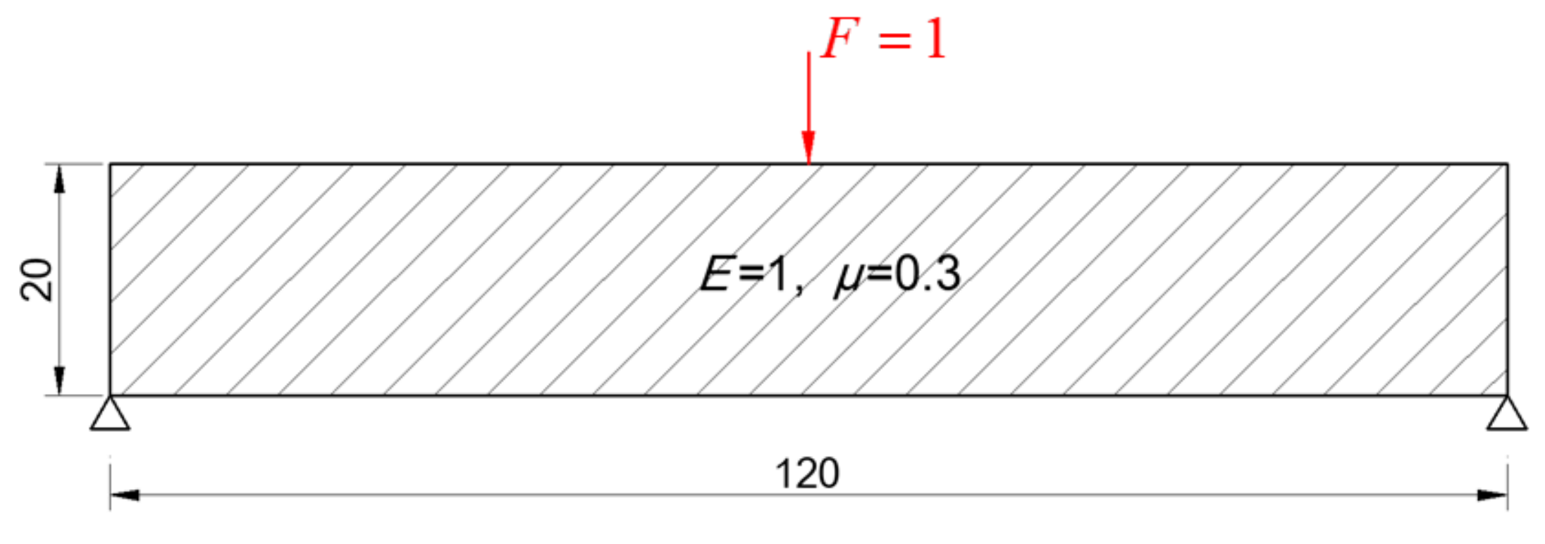
The MBB beam is a common model for topology optimization. The dimensionless beam with symmetric, simply supported ends is shown in Figure 5 and the unit load is applied at the middle of the top edge.

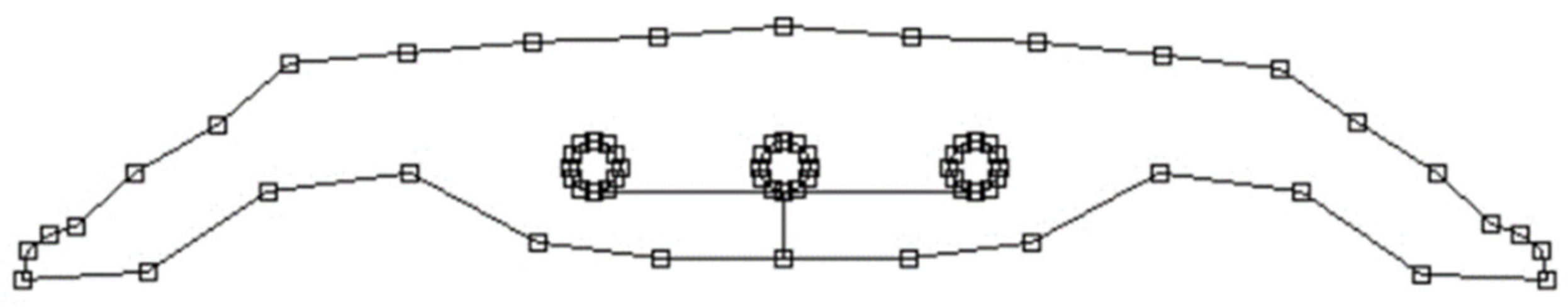
The constraint is that the volume ratio is less than 50%. The initial number of the control points is 36 and the two coordinates of a control point correspond to two design variables. The control points guarantee that the current solution domain must be within the initial boundary. When the volume ratio is less than 60%, the boundary optimization is completed and the inner structure optimization is carried out. Three holes with radii of 1 are generated at the appropriate positions according to the topological sensitivity. The circumference of each hole is divided into 12 segments and another 12 control points are added to the design variables to optimize the inner boundary, as shown in Figure 6. The initial circular hole is tiny and almost equal to a point. The circular hole gradually develops into an arbitrary shape according to the movement of the control points.

In addition, SIMP and LSM are also performed subject to the same constraints to verify the effectiveness of MBO. The design variables of these two methods are the densities of 2400 elements, and the minimal density is 0.001.

3.4.2. Design Results

The convergence processes of SIMP, LSM, and MBO are compared in Figure 7.

SIMP has the fastest convergence speed, while the convergence speeds of MBO and LSM are similar. The optimal structural compliances and volume ratios of SIMP, LSM, and MBO are compared in

Table 1. Optimization results.

	SIMP	LSM	MBO
Compliance	49.35	47.39	47.43
Volume ratio	50.0%	50.4%	50.0%

.

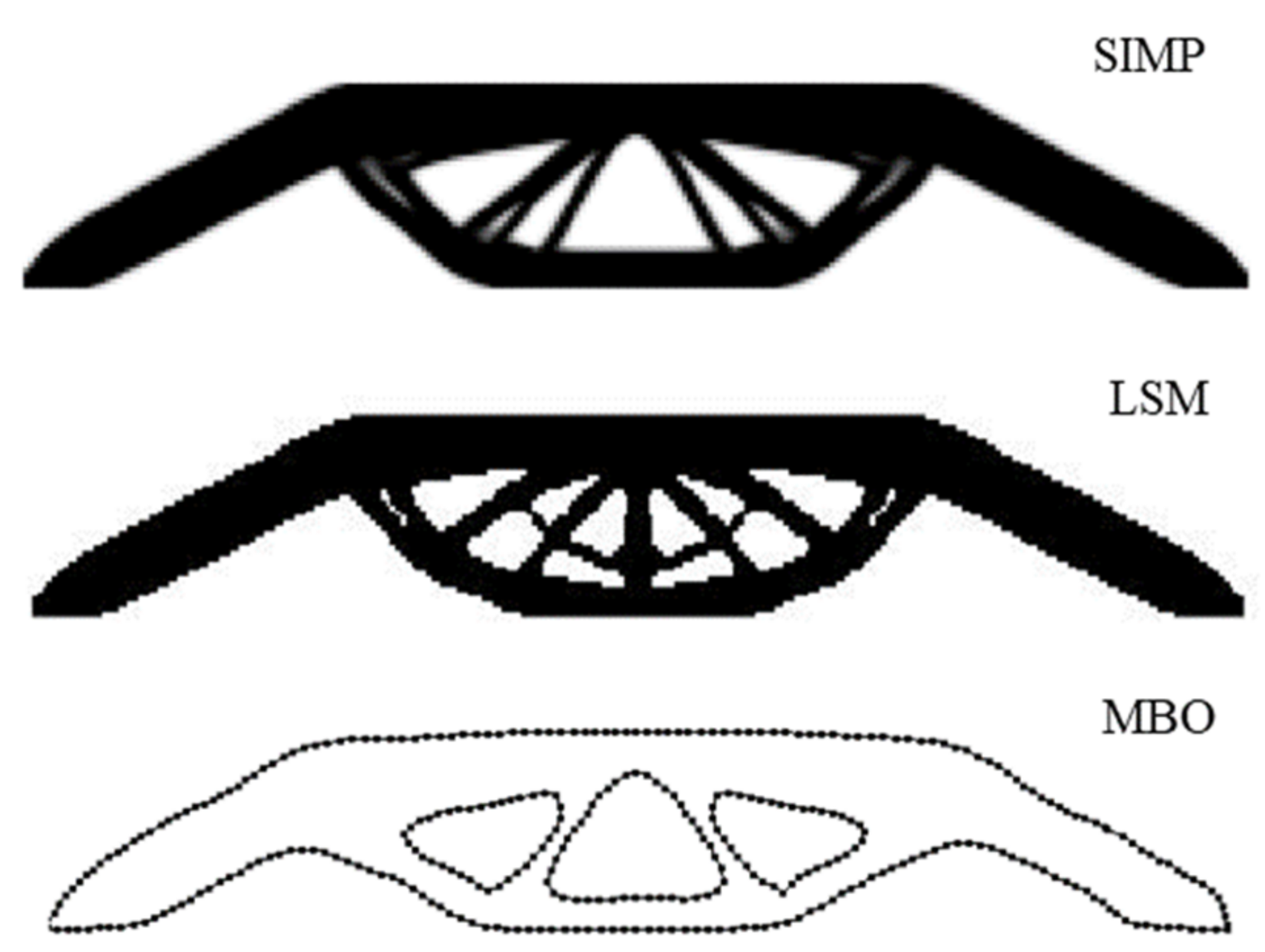
The optimal structural compliance of SIMP is the largest. The optimal volume ratio of LSM is larger than the constraint, and the volume ratio cannot be further reduced by adjusting parameters. The MBB beam structure optimization processes in the three methods are shown in Figure 8. SIMP, LSM, and MBO show their particular variation trends in the optimization process, and the final topological structures are similar.

According to the optimization results for the MBB beam, MBO can obtain better structural compliance than SIMP and a better volume ratio than LSM, so MBO shows an advantage in topology optimization.

3.4.3. Influence of Design Variables and Constraint

SIMP and LSM both have the problem of mesh dependence, so the influence of the number of design variables on the three optimization methods should be studied. The mesh density is increased by two times. The numbers of finite elements for SIMP and LSM are increased to 9600 and the initial number of control points for MBO is increased to 68. The optimization results are shown in

Table 2. Optimization results (increased design variables).

	SIMP	LSM	MBO
Compliance	50.01	49.38	48.06
Volume ratio	50.0%	50.1%	49.6%

.

The optimal topological structures are compared in Figure 9.

The optimization results for SIMP are quite different from the results for the original meshes. Holes appear in the solid beam structure of the original model. Compared with the results for LSM with the original meshes, the optimization is insufficient and many small beams appear, which can impact engineering applications. The optimization results for MBO show little difference from the previous results.

These three optimizations were performed on the same personal computer and the calculation times are compared in

Table 3. Optimization generation and calculation time.

	Coarse Mesh			Fine Mesh
	Variable	Time (s)	Generation	Variable	Time (s)	Generation
SIMP	2400	10.7	31	9600	699.1	100
LSM	2400	17.0	59	9600	293.9	48
MBO	72	309.0	100	136	326.0	100

. For an n-dimensional problem, when the mesh density increases by two times, the numbers of design variables for SIMP and LSM increase to $2^n$ times and the number of design variables for MBO increases to $2^{n-1}$ times. More design variables mean more time for the sensitivity analysis. Judging from the design results and the calculation time, SIMP and LSM are greatly influenced by the mesh density. With the increase in design variables, MBO gradually shows its advantages in optimization efficiency.

The influence of constraint on the three optimization methods is examined next. The optimizations are carried out subject to the constraints of a 60% and 40% volume ratio, respectively. Except for the volume constraint, the object function, design variables, and analysis conditions are the same as those in Section 3.4.1. The optimization results are shown in

Table 4. Optimization results (different constraints for the volume ratio).

	Constraint	SIMP	LSM	MBO
Compliance	40%	59.46	57.27	58.98
Volume ratio		40.0%	39.9%	39.9%
Compliance	60%	43.52	42.50	42.28
Volume ratio		60.0%	60.4%	59.9%

.

The optimal topological structures are compared in Figure 10.

The optimization results show that SIMP and LSM are greatly influenced by constraint and the number of design variables. MBO is more stable and has better boundary quality and less structural compliance.

3.5. Discussion

The SIMP, LSM, and MBO methods are compared according to the topology optimization results for the two-dimensional MBB beam. Then, the optimization stability of these three methods is preliminarily explored by adjusting the number of design variables and the volume constraint.

SIMP and LSM are limited by the mesh density and the volume constraint. Different conditions may lead to different results and the structural boundary may appear serrated, which requires manual smoothing. On the other hand, MBO is almost uninfluenced by them and has better optimization stability in simple two-dimensional problems.

MBO comprises shape optimization and topology optimization. For the MBB optimization, MBO can obtain a lighter result with smoother boundaries, which is more suitable for practical manufacturing.

It is more time-consuming for MBO to solve the problem with fewer design variables. However, with the increase in design variables, MBO needs much fewer parameters to describe the structure than FEM-based optimization, which helps MBO save much time in the sensitivity analysis.

The result of MBO can be pre-designed manually. In addition to automatically judging the hole numbers or the hole positions with the algorithm, they can also be specified manually. If the MBB beam is optimized using a symmetric four-hole topological structure, the optimum has a compliance of 48.28 and a volume ratio of 49.9%. The topological structure result is shown in Figure 11.

4. Topology Optimization of CRM Wing Structure

The topology optimization of the CRM wing structure is performed under asymmetric boundary conditions. The wing has a fixed support root and the external loads of the topology optimization are developed in the static aeroelastic analysis. The aeroelastic analysis of the wing structure needs to be analyzed repeatedly because its topological structure varies in each optimization generation.

4.1. Static Aeroelasticity

The static aeroelasticity is analyzed with an improved three-dimensional flight load that combines the high-order panel method and the meshfree method. The high-order panel method is employed for aerodynamic analysis and the meshfree method is employed for static analysis. The difference between the improved and basic three-dimensional flight load methods is that the static analysis is changed from FEM to the meshfree method. The method contains two iterative loops: the inner loop concerns the structural deformation convergence and the outer loop concerns the trim parameter convergence. More details about the basic three-dimensional flight load are introduced in the authors’ previous research [28,29]. The flowchart is shown in Figure 12.

The fight speed is 0.785 Ma at an altitude of 10,000 m and the dynamic pressure is 13,360 Pa. The static aeroelasticity is analyzed at a fixed angle of attack of 2°, so only the inner loop of the three-dimensional flight load is executed. After the static aeroelastic equilibrium is reached, the aerodynamic loads on the high-order aerodynamic panels are applied as the external loads to the wing structure to carry out the topology optimization.

The optimization object is the CRM wing structure, which is a common research model for aerodynamic and aeroelastic research, as shown in Figure 13. The half span is 29.38 m, the root chord is 11.87 m, and the taper ratio is 4.34. The sweep angle of the leading edge is 37.23° and the dihedral angle is 4.85°. The material of the wing is 7075 aluminum alloy, the elastic modulus is 71.7 GPa, the Poisson ratio is 0.33, and the material density is 2700 kg/m³.

The structural model is adjusted to satisfy the requirements of topology optimization. The wing shape remains unchanged and the inner space is filled. Some ribs are reserved to maintain the shape and transfer flight loads. The stiffness matrix of a three-dimensional wing structure is extremely huge, so, limited by the calculation conditions, only the red inner wing segment is optimized and the green segment is used for aeroelastic analysis.

4.2. Design Strategy

The design object is expanded from a two-dimensional beam to a three-dimensional wing. SIMP and MBO are carried out to compare the optimization results. The aerodynamic shape of the CRM wing remains unchanged and only the inner topology structure is optimized.

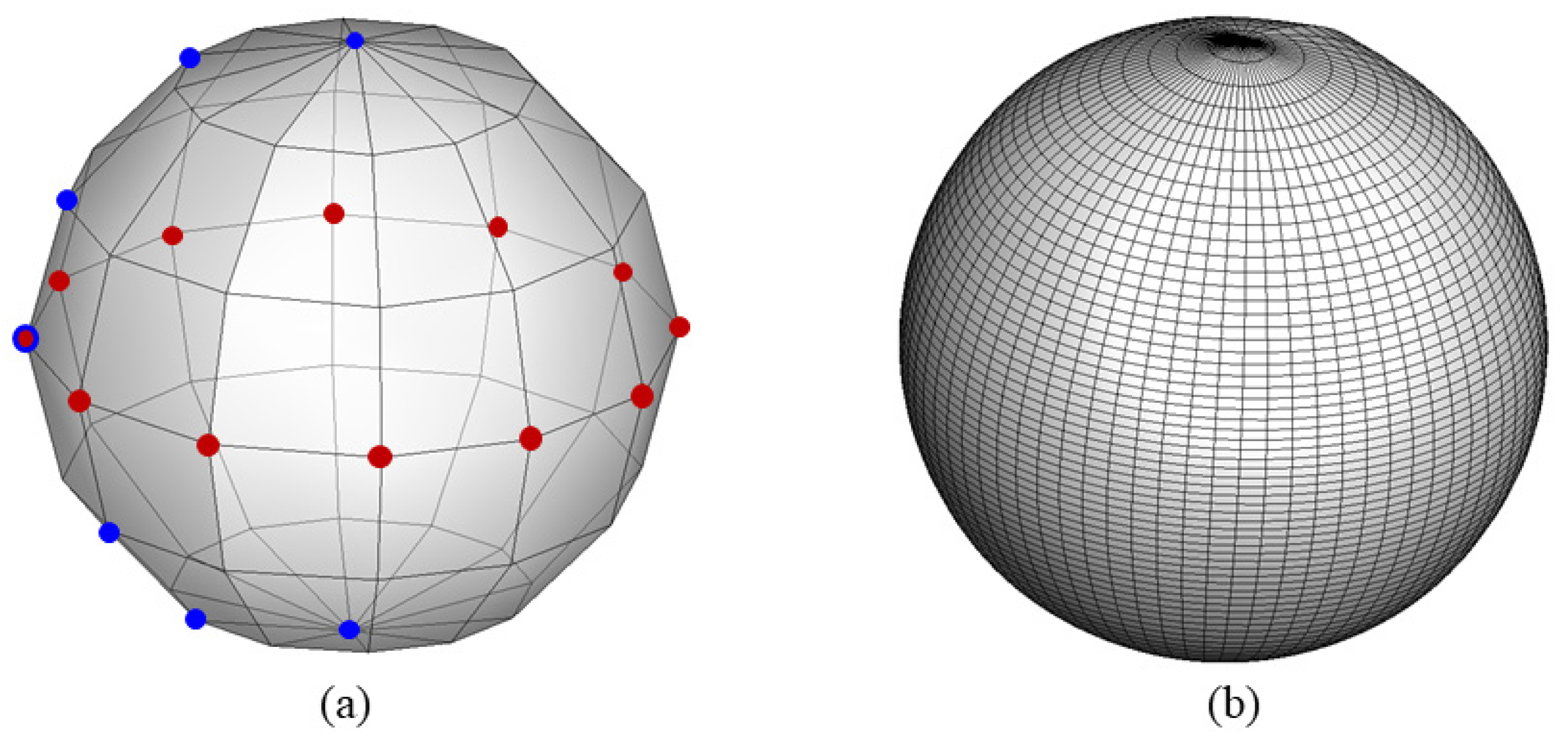
In the MBO method, the inner holes of the wing structure are controlled by the NURBS surfaces and the hole shapes vary with the coordinates of the control points. A sphere hole, like the earth, is described by 2 poles, 12 longitude lines, and 5 latitude lines. The distribution of the 62 control points is shown in Figure 14a and the initial spherical hole shape with a radius of 1 described by these control points is shown in Figure 14b.

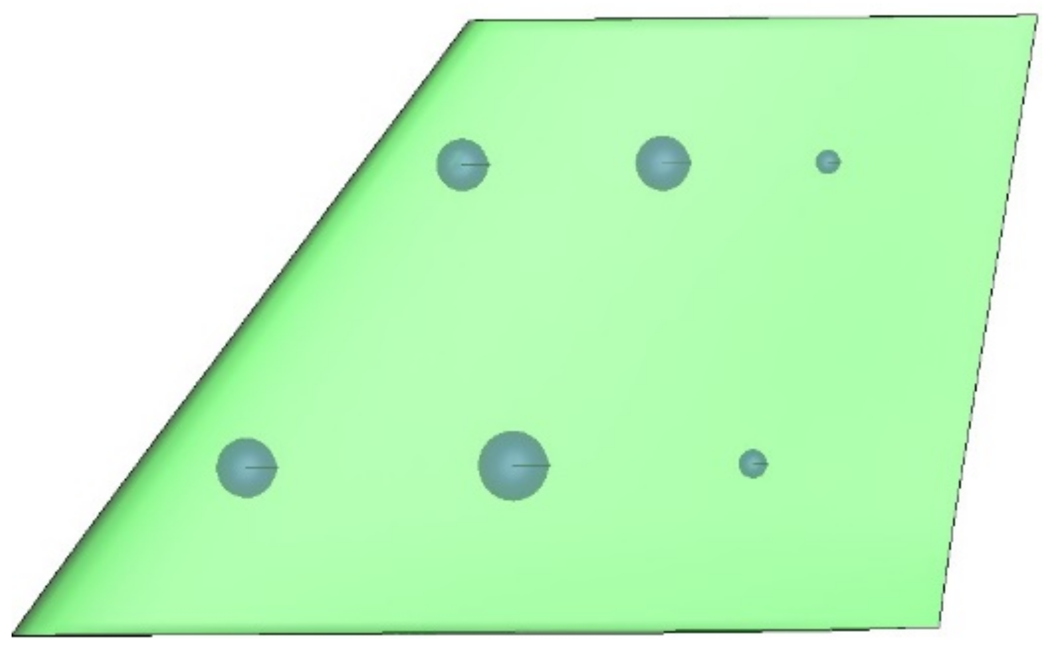
The sphere centers are can be automatically generated by the algorithm or specified manually. In this research, six initial sphere centers are specified at the inner segment of the wing, as shown in Figure 15. The initial sphere holes in Figure 15 are a little exaggerated to display them more clearly. They are tiny and almost point-like. A sphere hole gradually develops into an arbitrary shape with the movement of its control points. The moving direction of a control point is determined by its compliance sensitivity and volume sensitivity. Therefore, the number of design variables is 372 in total.

The optimization flowchart is similar to that described in Section 3.3 and the external loads used in the topology optimization are updated by the three-dimensional flight load in each generation, as shown in Figure 16. The object is the minimal structural compliance and the volume ratio constraint is 50%.

4.3. Design Results

The design results for MBO and SIMP are compared in

Table 5. Optimization results for MBO and SIMP.

	Design Variable	Compliance	Volume Ratio	Generation
MBO	372	9.426 × 107	49.57%	65
SIMP	18,000	9.420 × 107	50.00%	27

.

The final topological structure optimized by MBO is shown in Figure 17a and the basic configuration extracted from the optimization result is shown in Figure 17b. The MBO result tends toward an integral panel wing structure and retains the thick skin. The interior is a honeycomb-like support structure and the support beams are perpendicular to the rib, which is conducive to improving the structural stiffness. The configuration is consistent with the form of the integral panels commonly used in aircraft wing surfaces, and the boundary is relatively smooth.

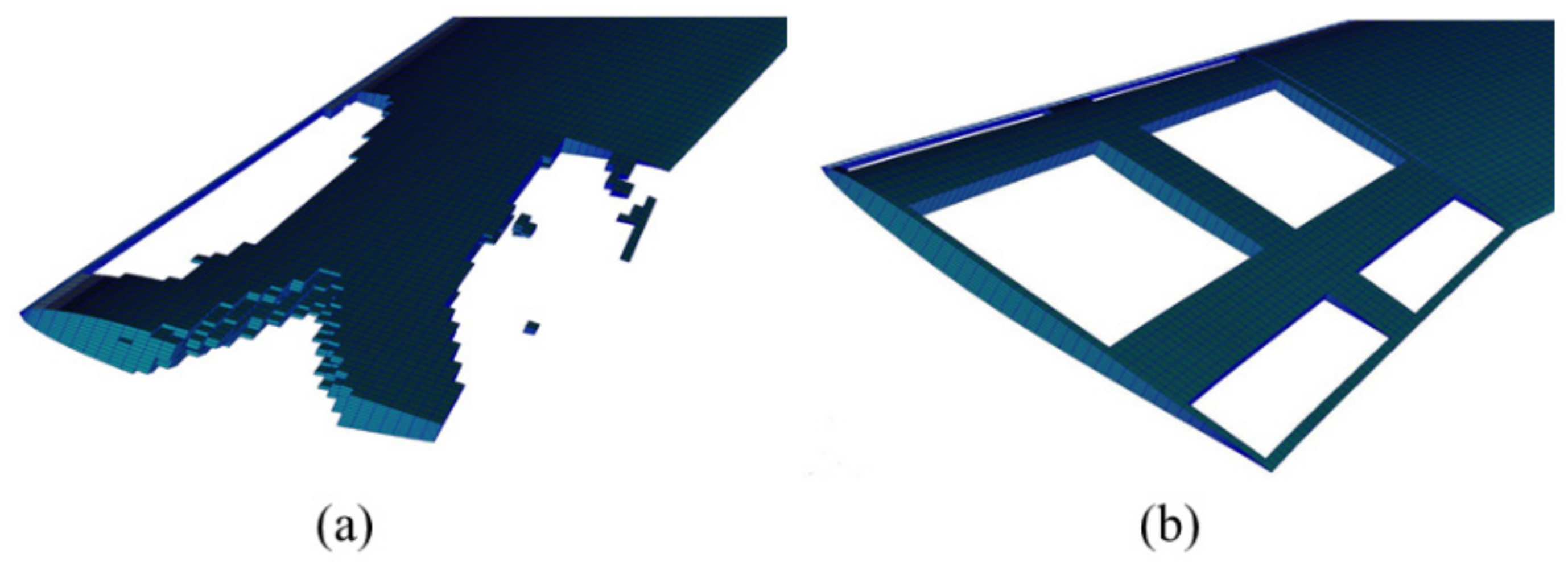
The final topological structure optimized by SIMP is shown in Figure 18a and, with regard to the beam positions of the CRM wing structure, a double-beam configuration of the inner wing segment with a 50% volume ratio is designed, as shown in Figure 18b.

In the SIMP result, the wing structure changes from a double-beam configuration to a single-beam configuration, and holes appear in the middle of the front beam. The structural compliance of the CRM structure is 9.865 × 10⁷ and the volume ratio is 50.44%. The results show that topology optimization can help reduce structural compliance.

4.4. Discussion

MBO is preliminarily applied to a three-dimensional CRM wing structure and, as a comparison, SIMP is also performed with the same conditions.

The optimization results of MBO and SIMP have similar levels of compliance, but the structural boundary of MBO is smoother and flatter. The clear structure of MBO is more suitable for engineering practice than SIMP.

Compared with SIMP, MBO has poor computational robustness and unstable results. The calculation codes of the meshfree methods need to be further improved and optimized.

For the problem of a three-dimensional complex structure, some particular boundaries, edges, and corners with large curvatures are difficult for the current NURBS curves and surfaces to describe. They should be further designed in the subsequent shape and size optimization.

5. Conclusions

A moving boundary meshfree topology optimization that combines the Galerkin method of weighted residuals and NURBS is presented in this paper.

The proposed method was first applied to the two-dimensional MBB beam. Compared with the results of the FEM-based methods, the moving boundary optimization could obtain more than 3.5% compliance reduction subject to the same constraints. The shape constraints were conveniently applied and the optimized boundary was smoother. The proposed method only needed 2% of the design variables of the FEM-based methods or fewer, which helps reduce the time taken for sensitivity analysis and improves the optimization efficiency. Furthermore, the moving boundary method was almost unaffected by mesh density, the number of design variables, and constraints. The optimization stability makes it more flexible in dealing with two-dimensional problems.

Then, the proposed method was applied to the inner segment of a three-dimensional CRM wing structure, considering the aeroelastic effect. The moving boundary optimization needed 2% of the design variables of the FEM-based method and obtained the prospective compliance subject to the same constraint. The optimal wing structure was clear and close to the double-beam configuration in practical engineering. The proposed method was still efficient for the three-dimensional wing structure.

As a new topology optimization method, there is still a big gap between the proposed method and commercial FEM-based software in terms of robustness and applicability with complex structures. Some regions with large curvatures need to be described more exactly in the meshfree method. The program codes need to be further improved and optimized. The moving boundary technique has great research value and broad development prospects. Our future research will focus on the above key points.