
On the Indispensability of Isogeometric Analysis in Topology Optimization for Smooth or Binary Designs


Abstract
:1. Introduction
2. Discussion of the Problems in FEM-Based Topology Optimization Works
2.1. Smooth or 0–1 Designs in Topology Optimization
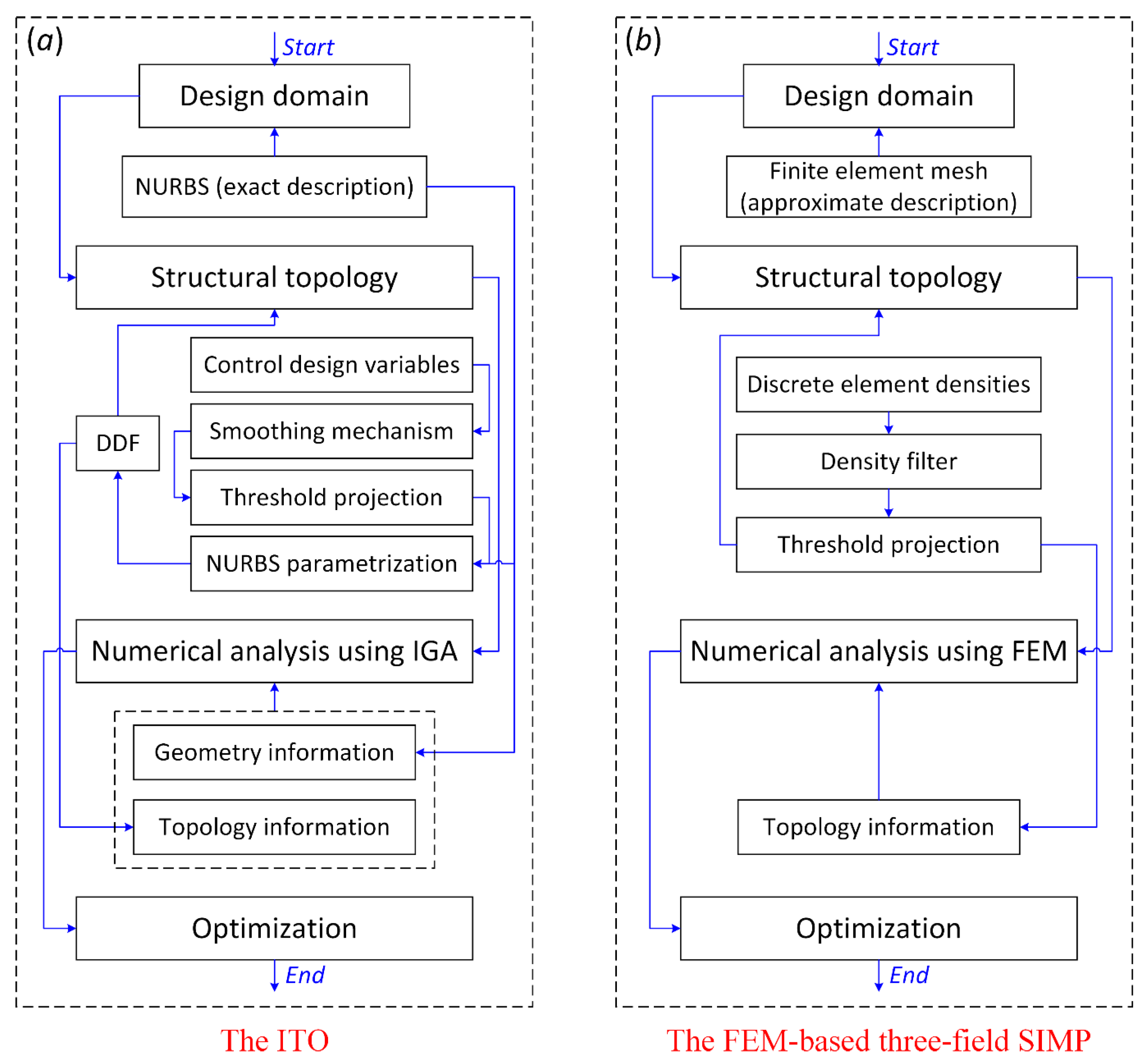
2.2. FEM-Based Three-Field SIMP Method
2.2.1. A Brief Description
2.2.2. Several Critical Problems
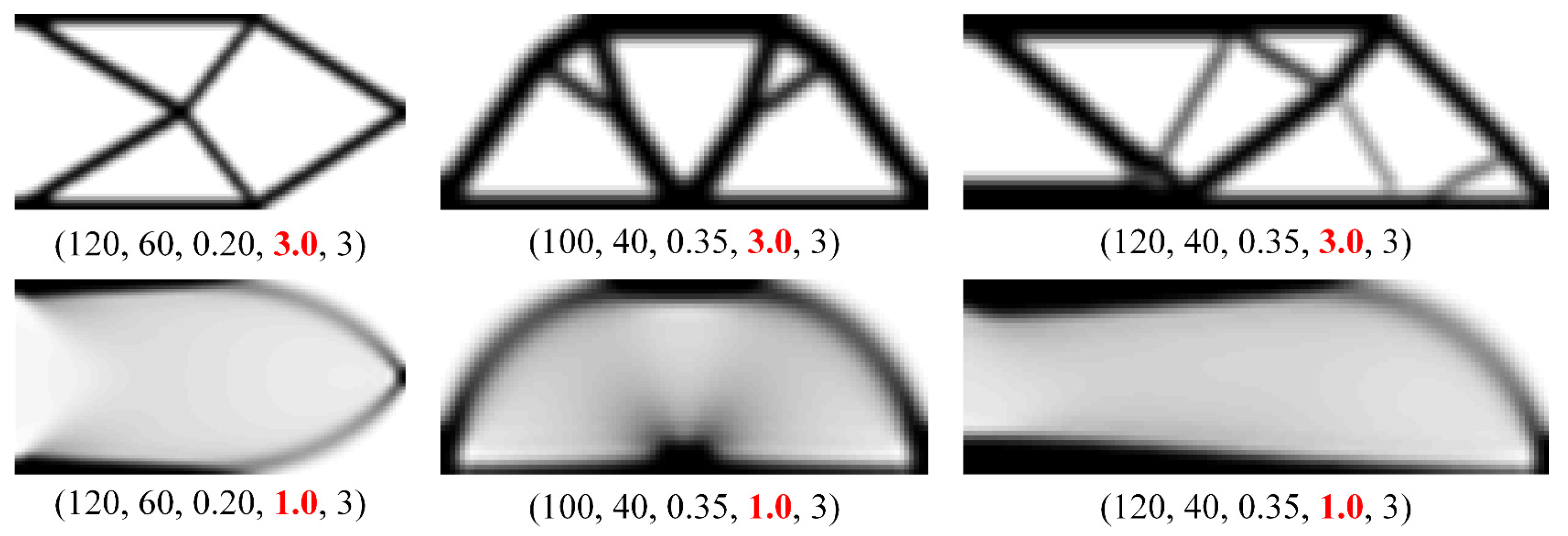
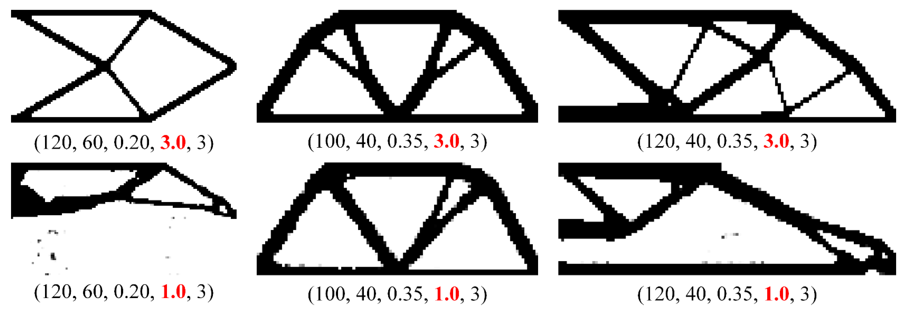
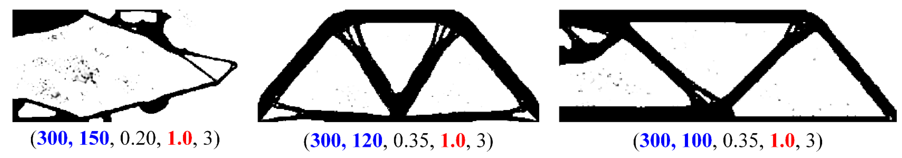
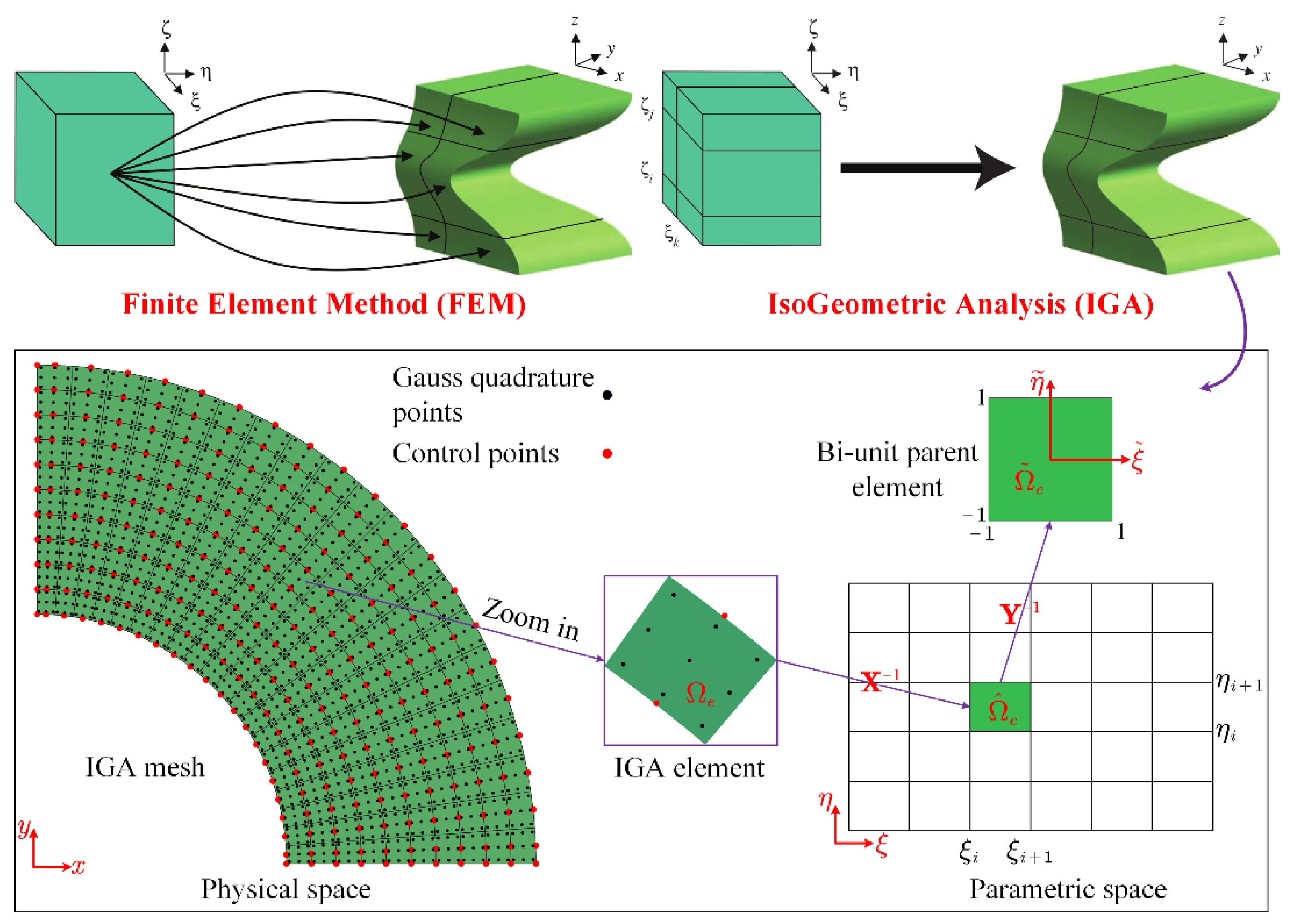
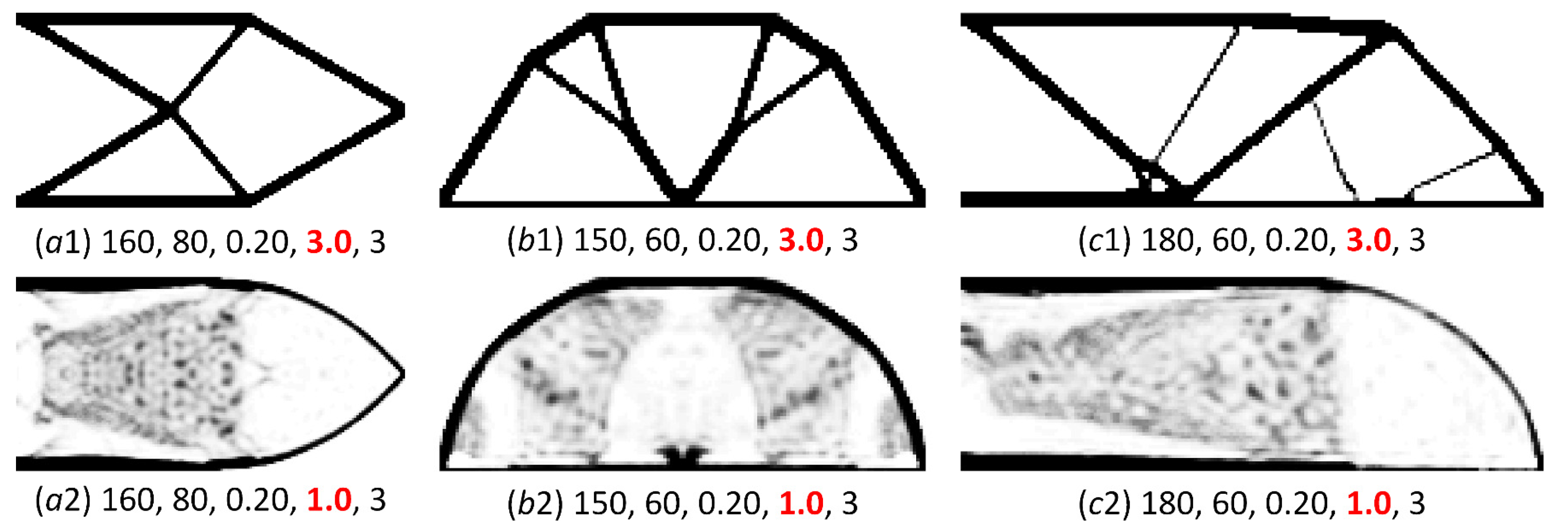
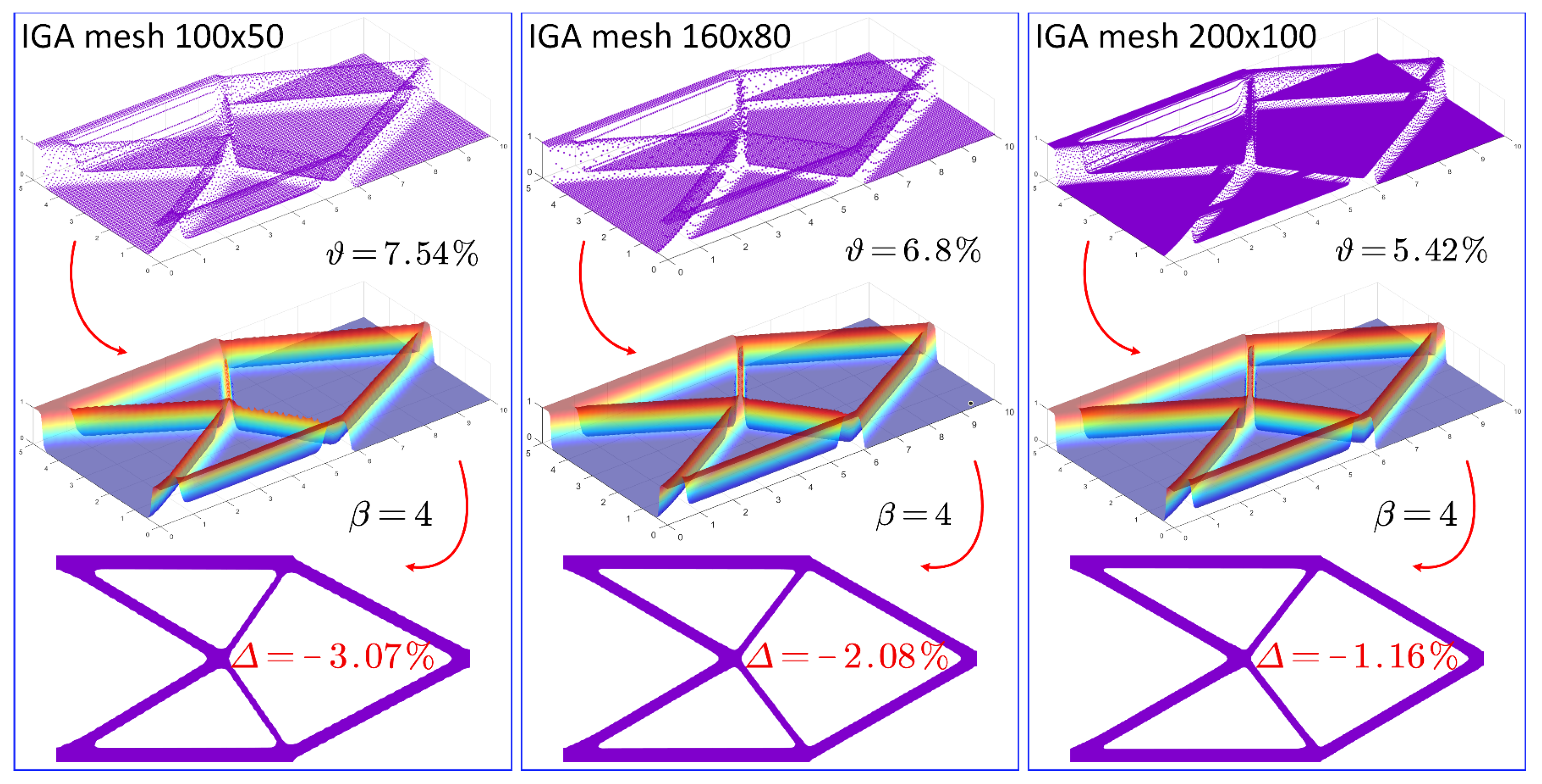
- As shown in Figure 4, if the design domain uses a denser mesh, the numerical precision is improved and the optimization with the ersatz material model and threshold projection can find relatively appropriate designs. This reveals that numerical precision has a significant influence on the ability of threshold projections to generate structural topologies. However, increasing the number of finite elements results in a prohibitive computational cost, Although the optimization can find solutions to some extent, the densities dramatically change in the optimization and cannot converge in a stable process. Hence, the use of IGA to unify CAD and CAE in an integrated model with greater numerical precision at the same finite elements can offer a powerful alternative to FEM for solving unknown responses [40,41].
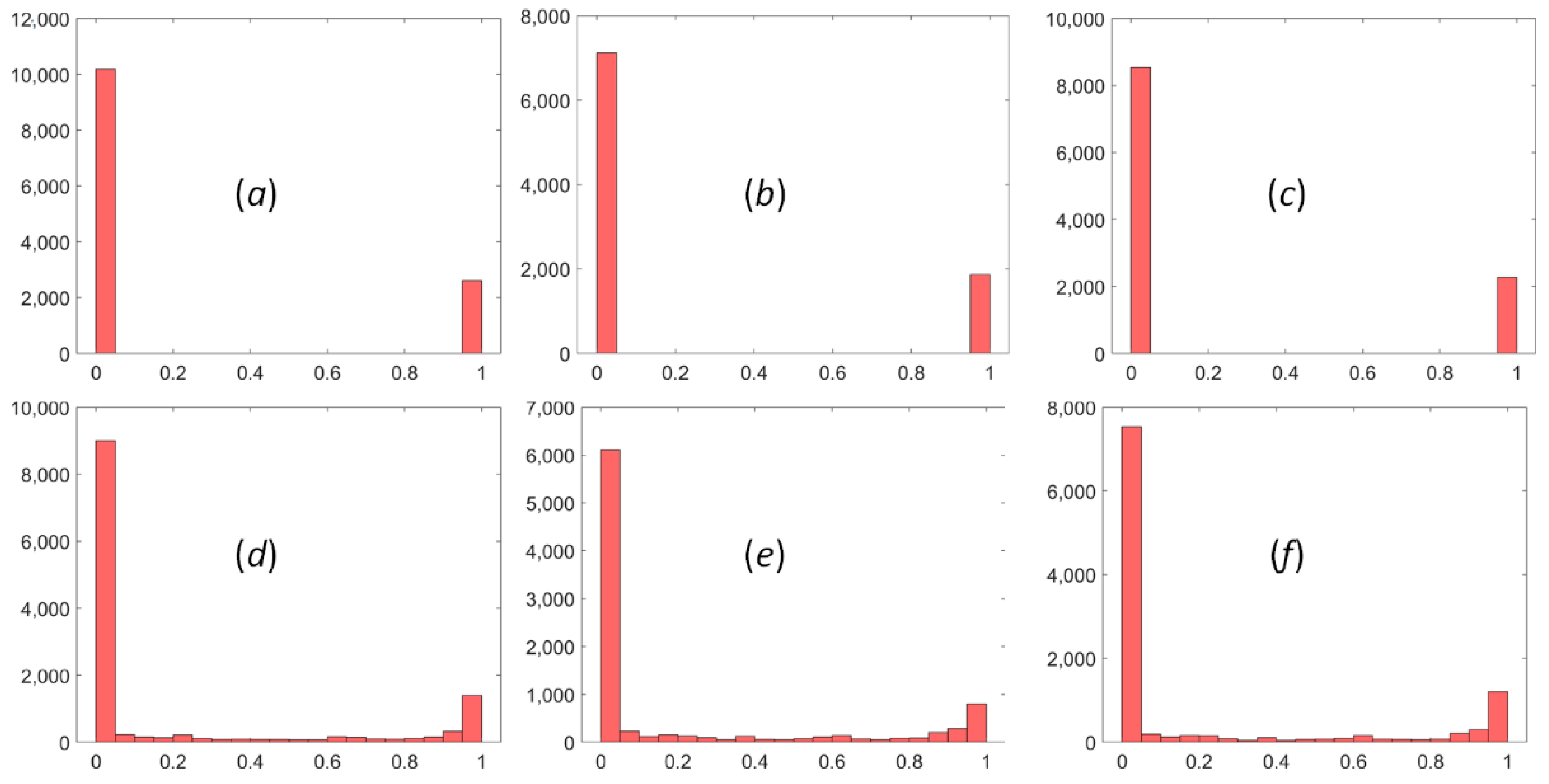
- Previous works [29,30] revealed that the ersatz material model is more suitable for optimization to obtain a smooth design in the density framework and the material penalization model can further benefit the optimization to obtain a pure 0–1 design. Meanwhile, the threshold projection is introduced to define the floating constraint to push the design variables towards 0 or 1. In fact, the material penalization model, with its overestimation of structural compliance, leads to numerical deviations in the structural stiffness of the final topologies, and a unified topology optimization based on the ersatz material model, using the density to produce smooth designs and pure 0–1 designs is more meaningful. Moreover, the floating constraint increases the numerical difficulties of the optimization. It is imperative to define the projection mechanism in the density distribution.
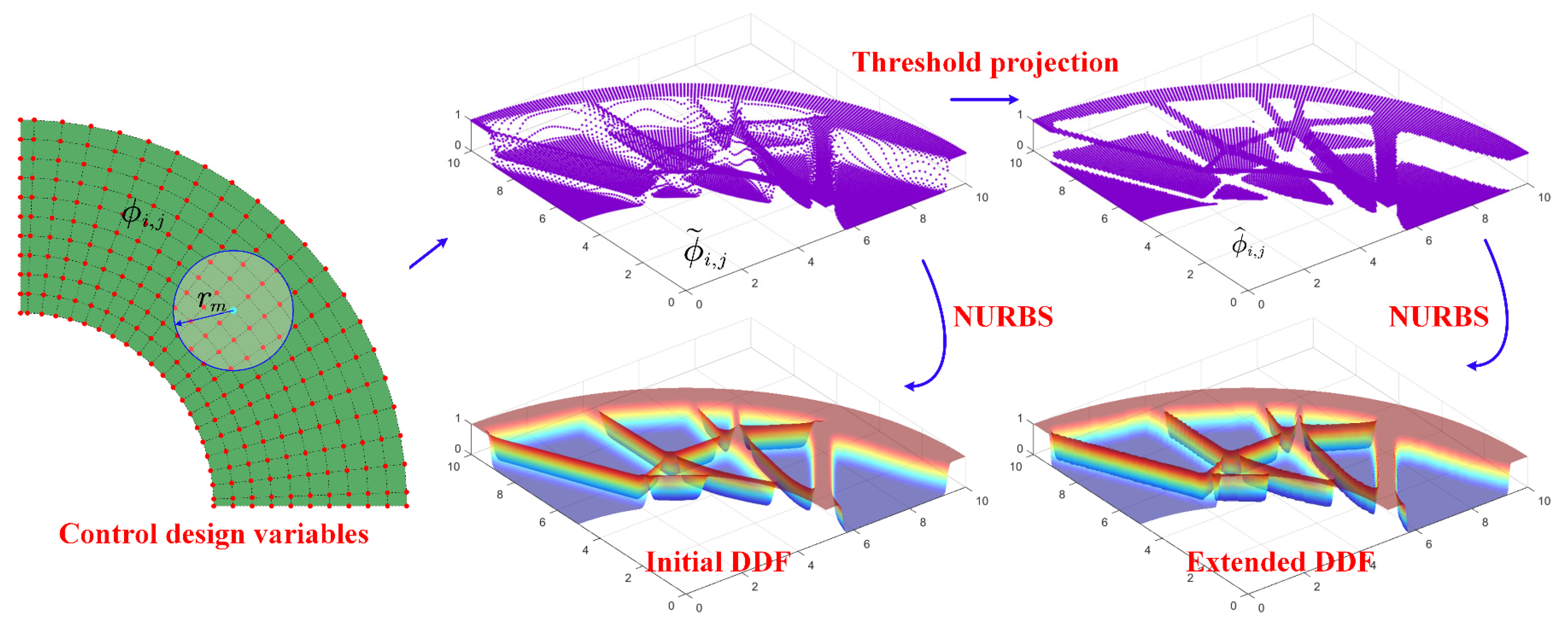
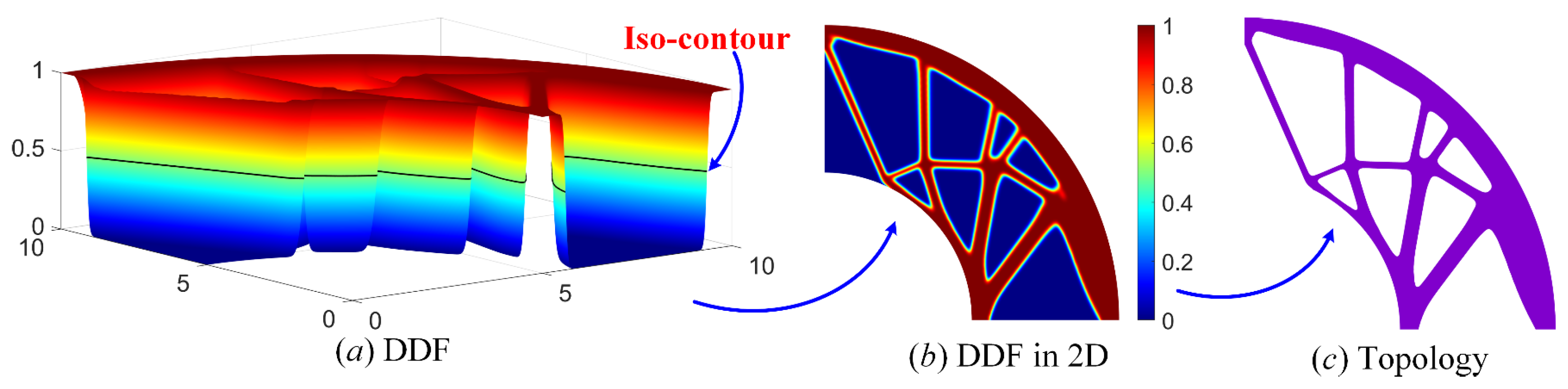
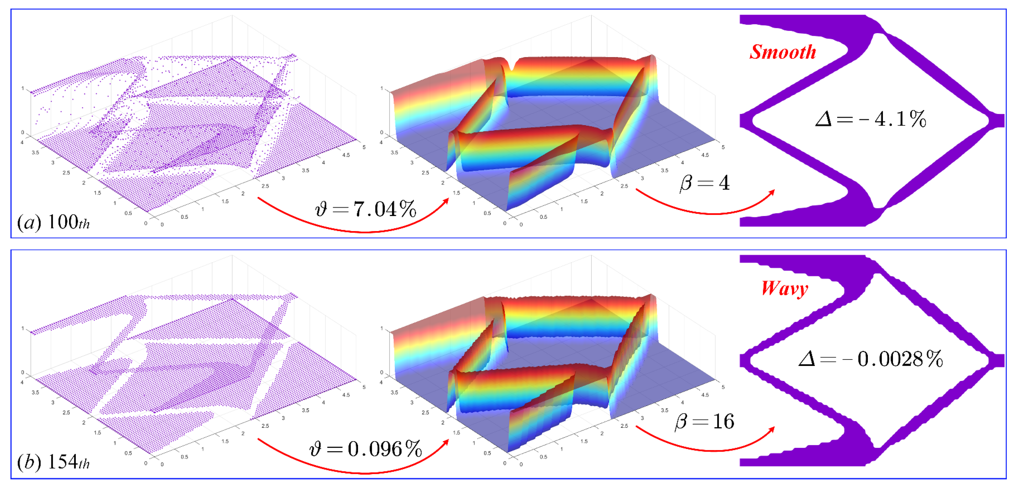
- It is imperative to construct a more effective DDF to represent the structural topology with smoothness by using NURBS approximation mechanism rather than the Lagrange interpolation. Furthermore, the DDF can combine with the threshold projection to extensively remove the intermediate densities in the transition area, and the optimizer can avoid the discrete characteristic in the topology description using the DDF. Additionally, during the optimization, the DDF with the implicit representation of structural boundaries is applied to describe the structural topology, and the DDF at the Gauss quadrature points is utilized in IGA to evaluate the material elastic properties. Hence, the current ITO can eliminate the considerable dependence on elementary densities in previous works.
3. ITO with an Extended DDF
3.1. An Extended DDF to Implicitly Represent Structural Topologies
- Step 1: Introducing the design variables at the control points, namely the control-design variables:
- Step 2: Using the smoothing mechanism to improve the overall smoothness of the control-design variables:
- Step 4: Using NURBS to construct a density-response surface for the design domain:
3.2. NURBS-Based IGA
3.3. Comparisons between the ITO and the FEM-Based Three-Field SIMP
4. The Problems of Compliance-Minimization and the Compliant Mechanism
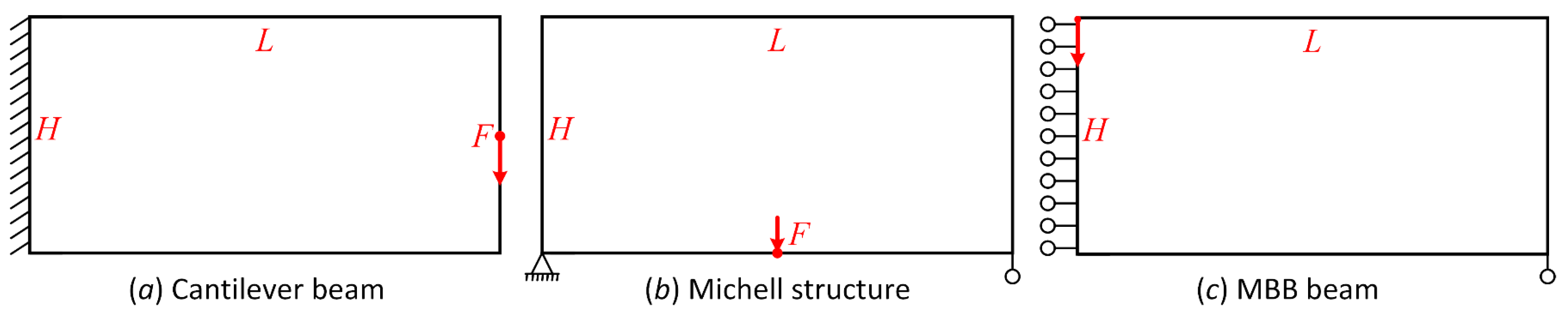
4.1. Compliance-Minimization Formulation
4.2. Compliant Mechanism Design Formulation
5. Numerical Examples
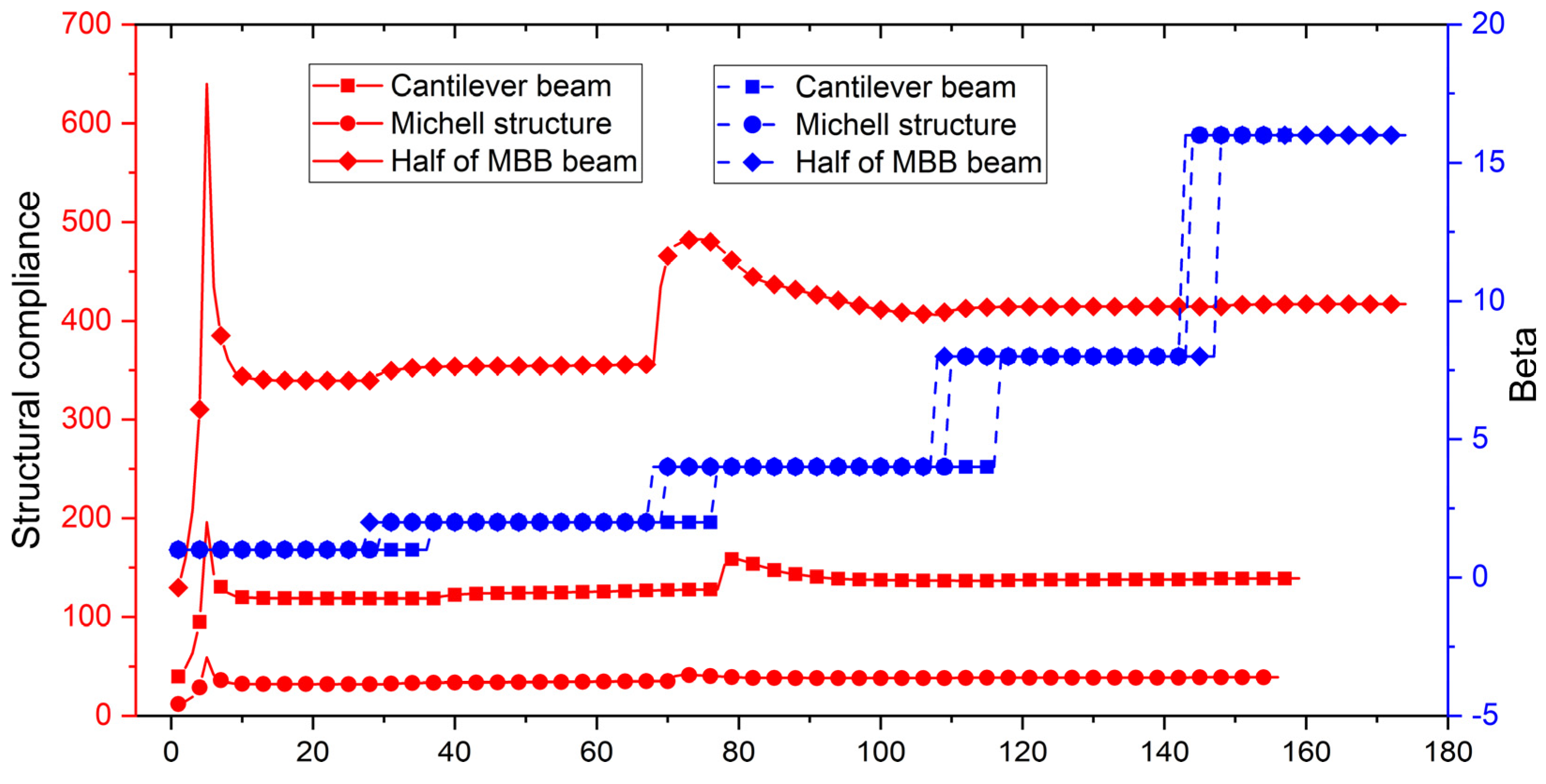
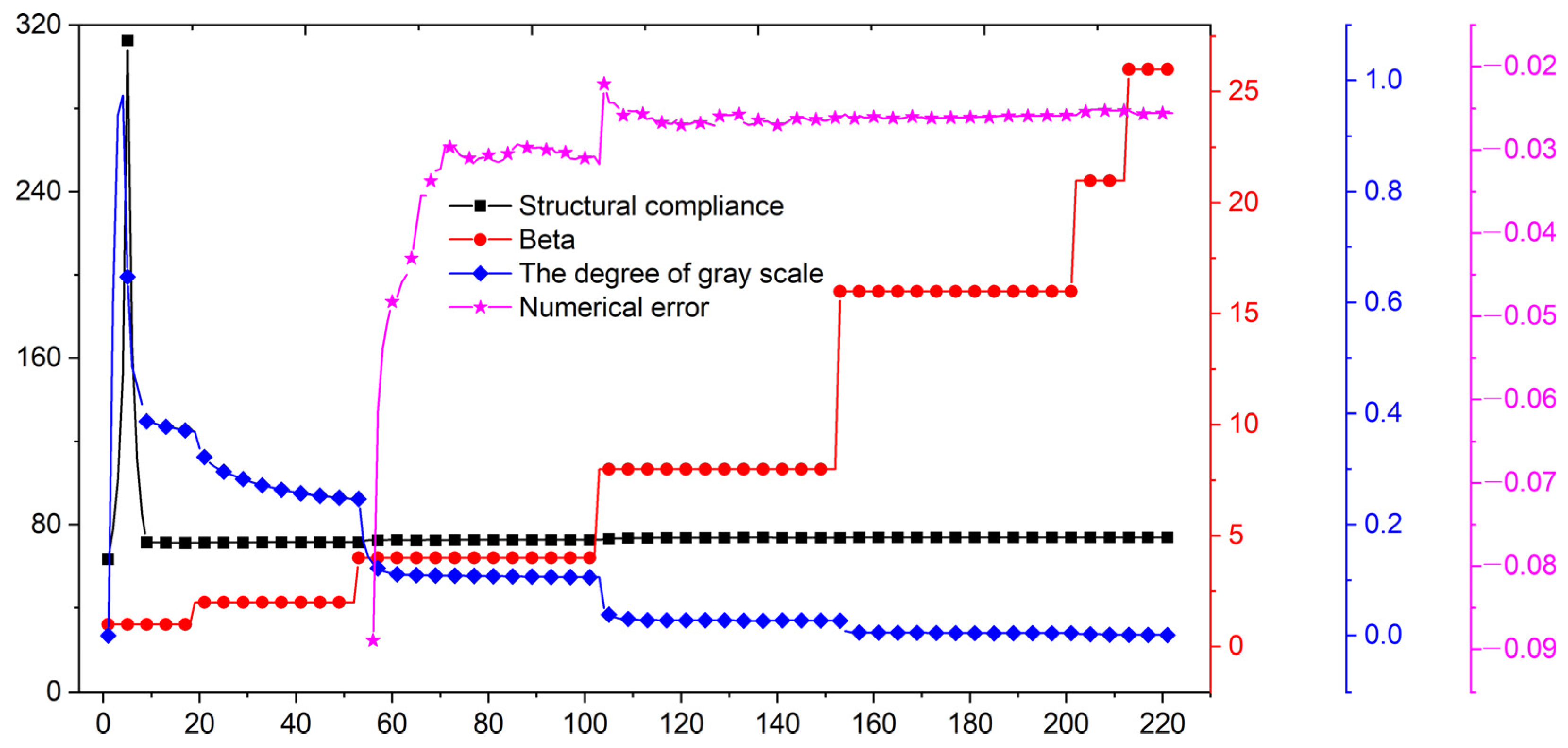
| Algorithm 1.The iterative algorithm in the code for the parameterin threshold projection. |
| if loop <= 200 if beta < 10 && (loopbeta >= 40 || change <= 0.01) beta = beta*2; loopbeta = 0; change = 1; end else if beta < 128 && (loopbeta >= 20 || change <= 0.01) beta = beta + 5; loopbeta = 0; change = 1; end end |
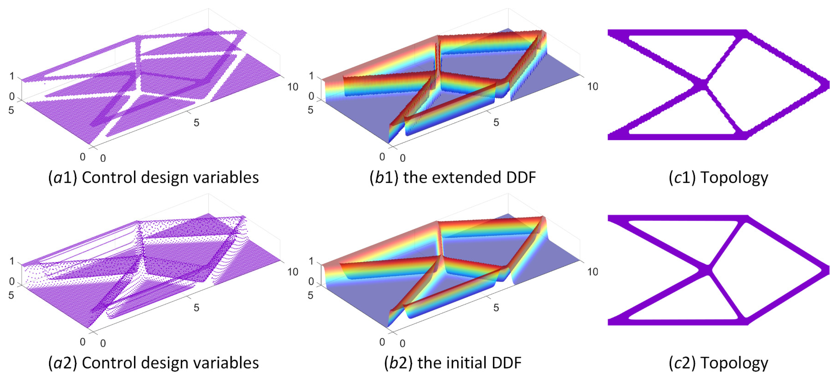
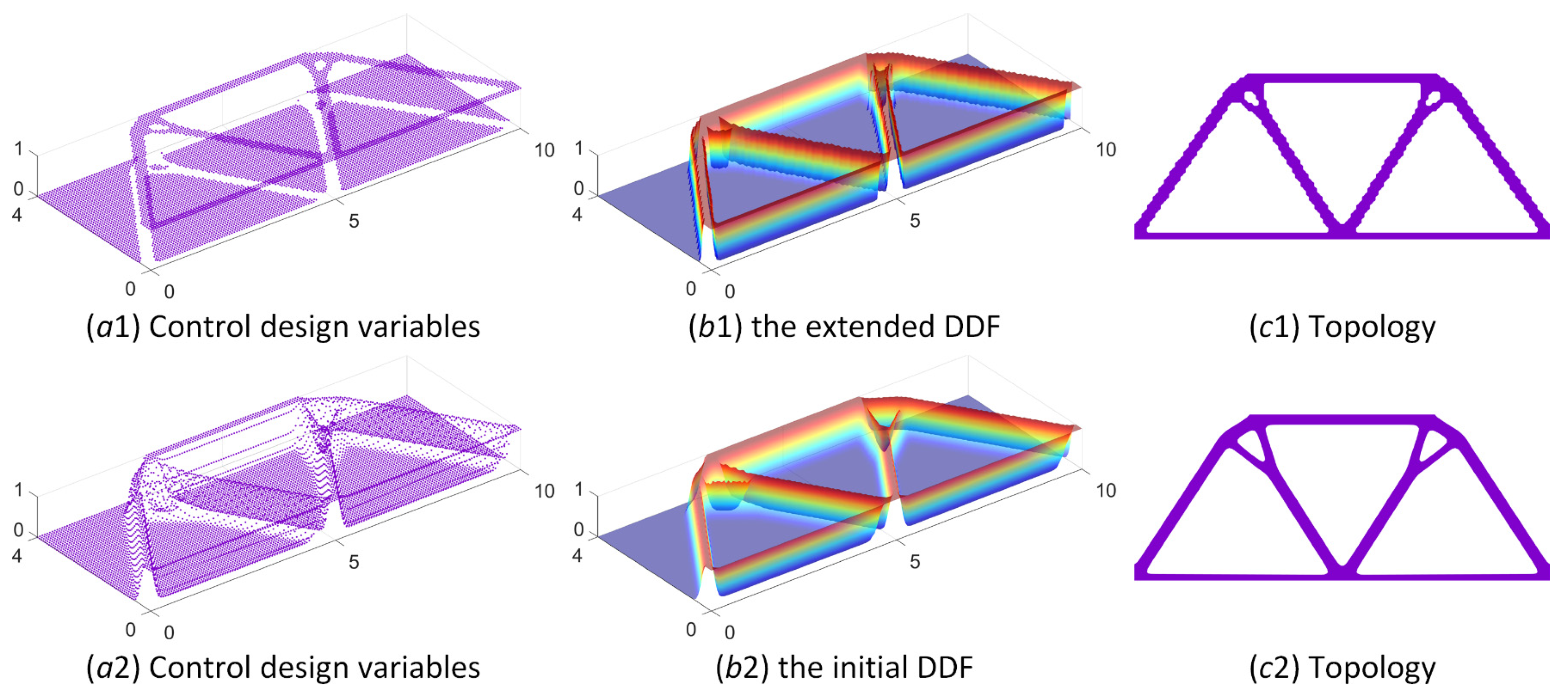
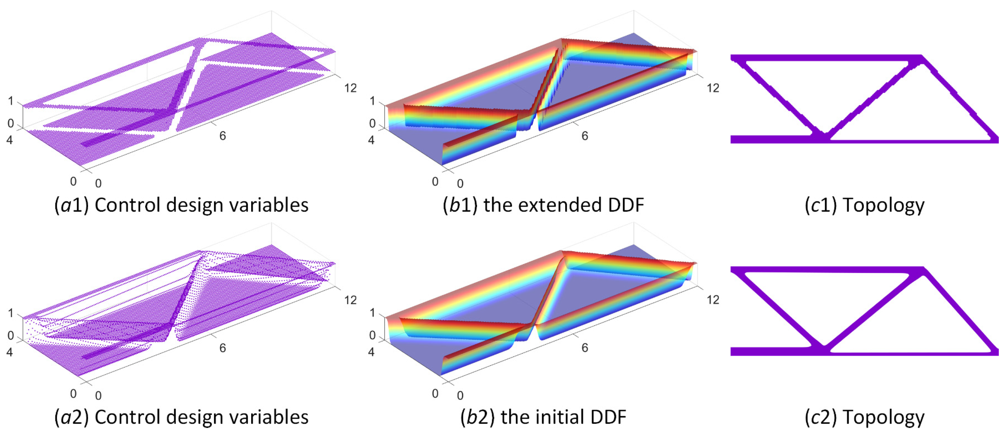
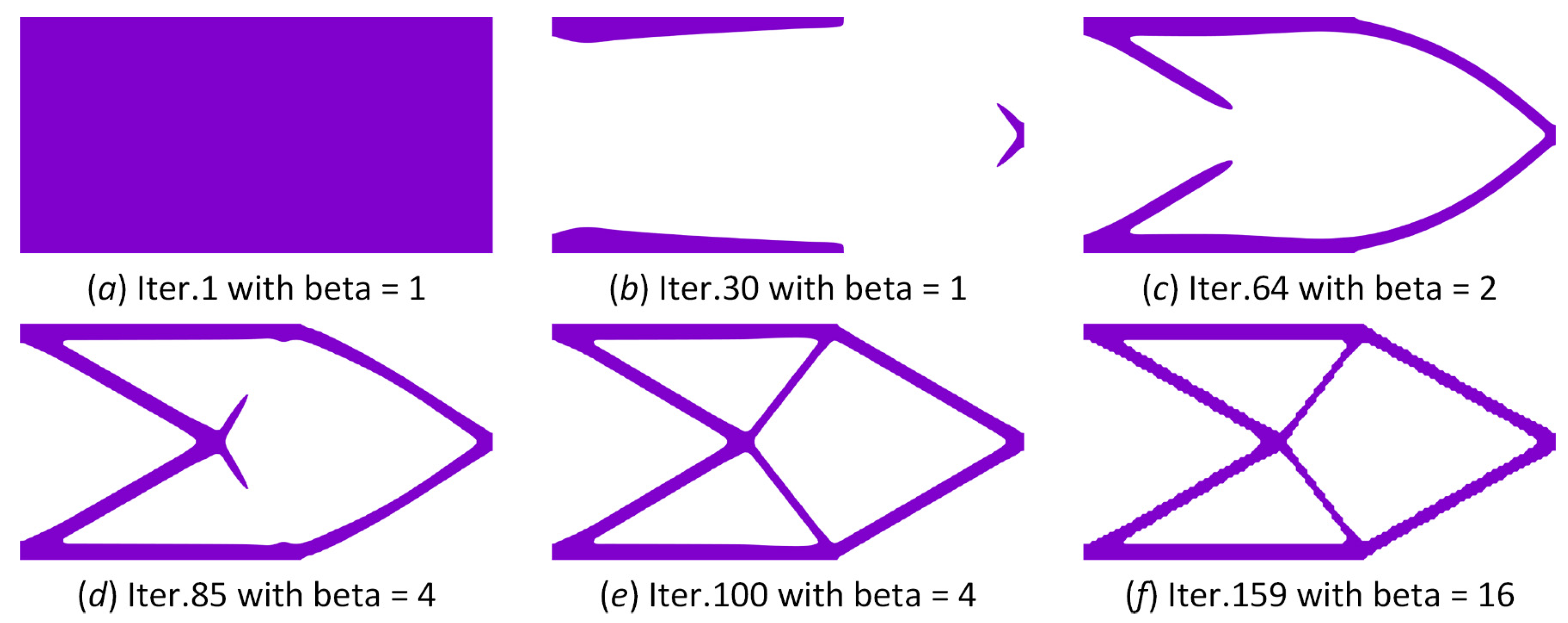
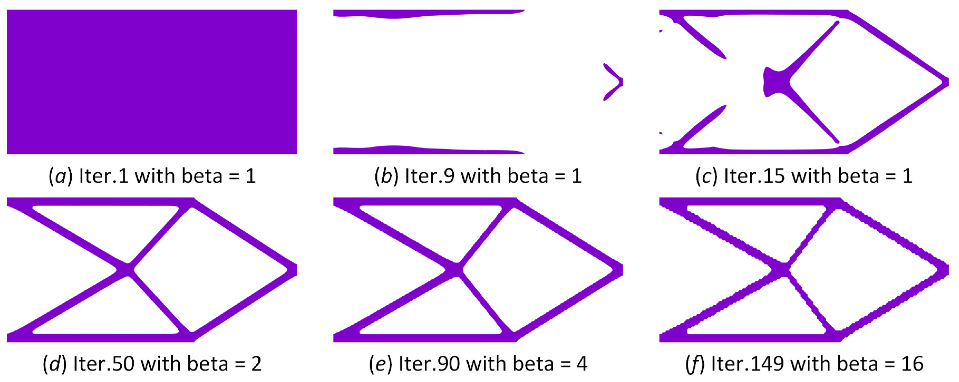
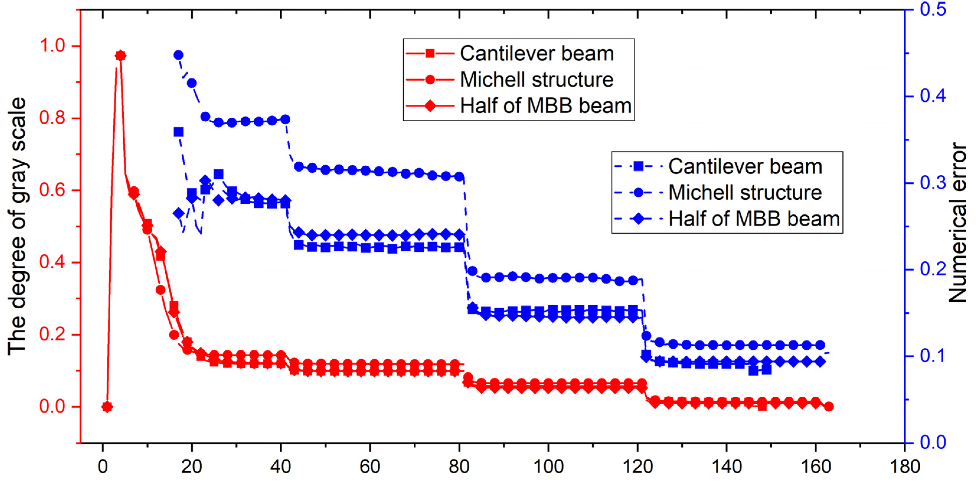
5.1. The Effectiveness of the Extended DDF
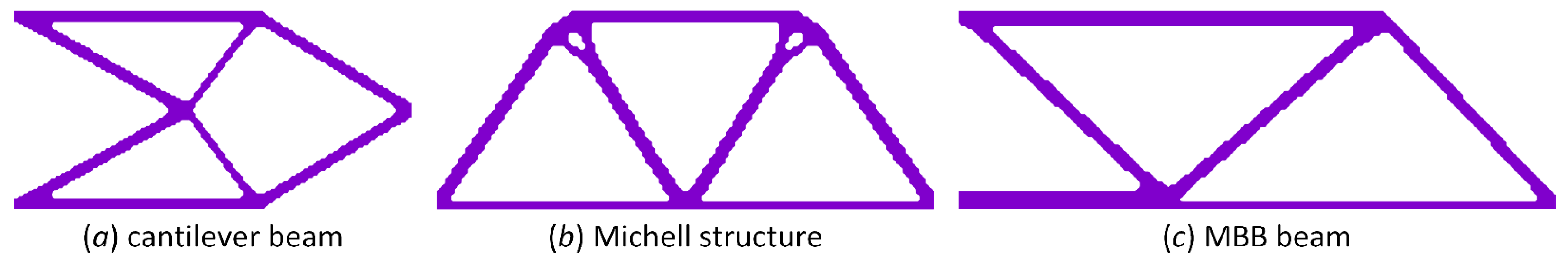
5.2. The Indispensability of the IGA in Replacing the FEM in Topology Optimization
5.3. The Effectiveness of the Ersatz Material Model Compared to the Material Penalization Model in the ITO
5.4. Discussion of the Influence of the IGA Mesh
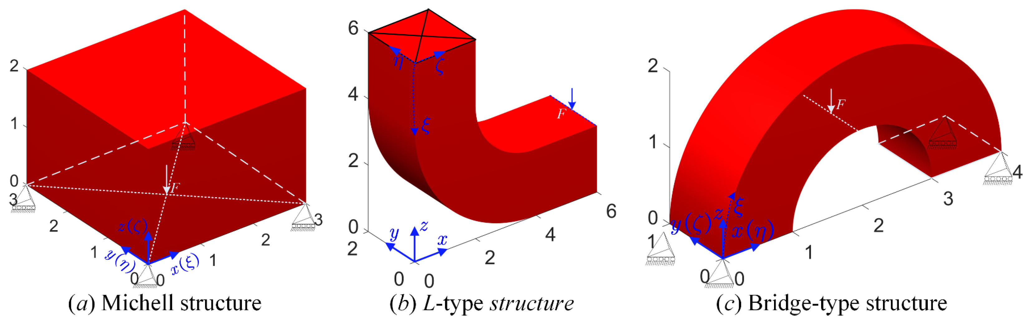
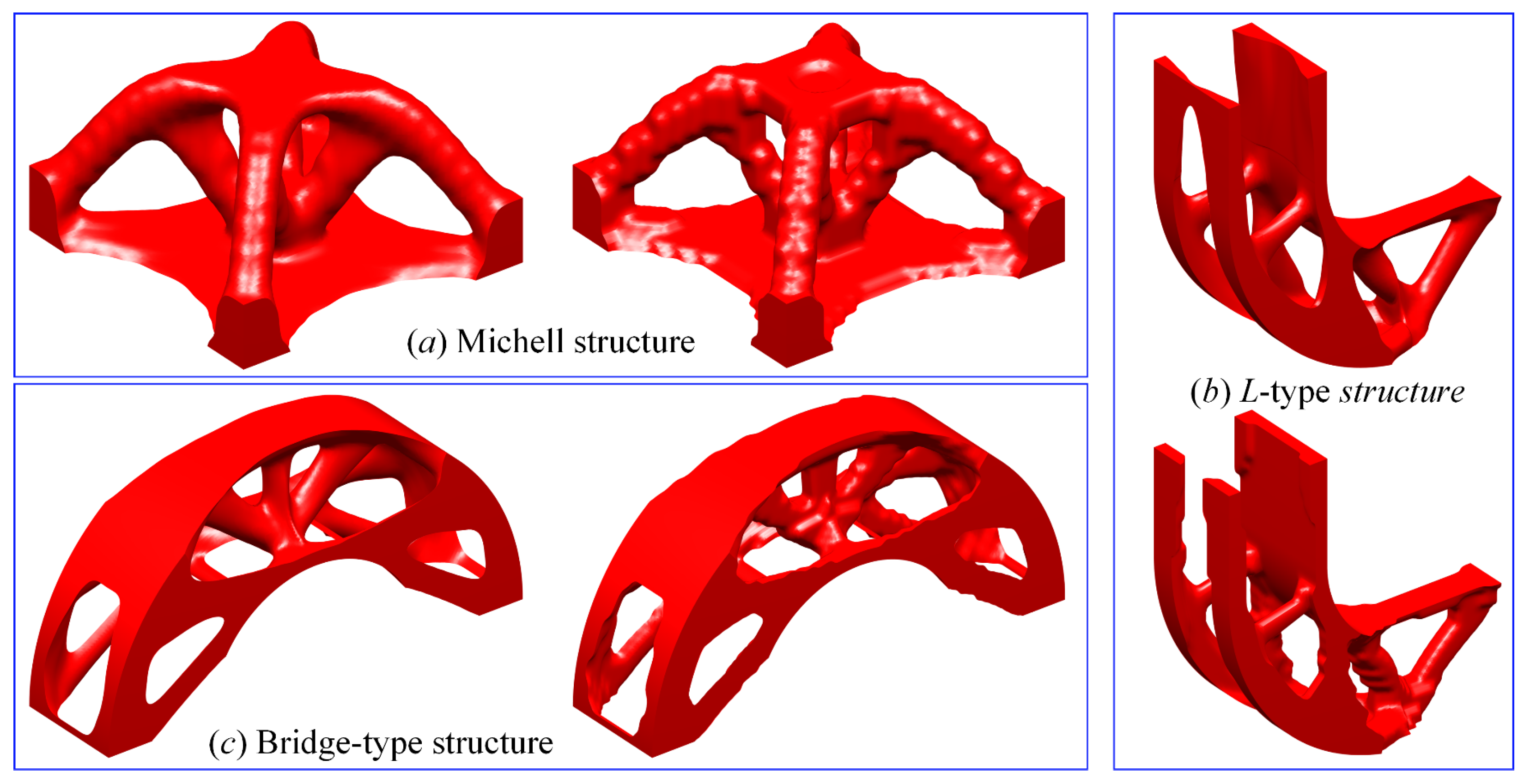
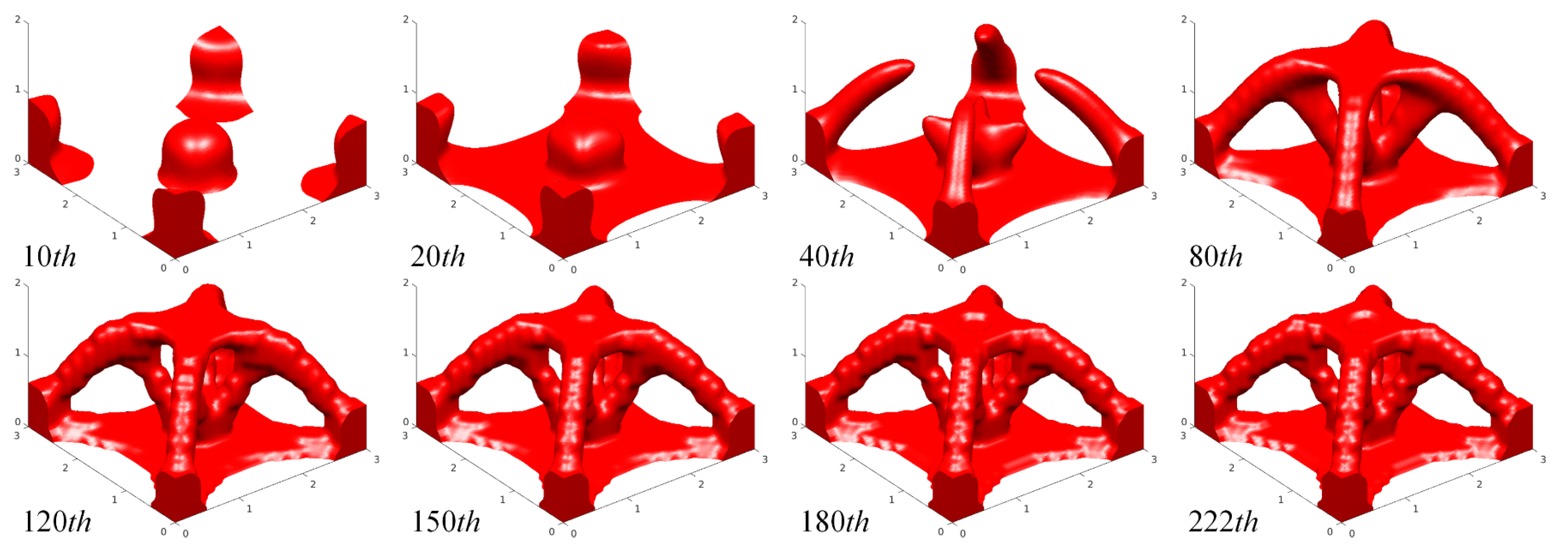
5.5. Stiffness-Maximization Designs in 3D
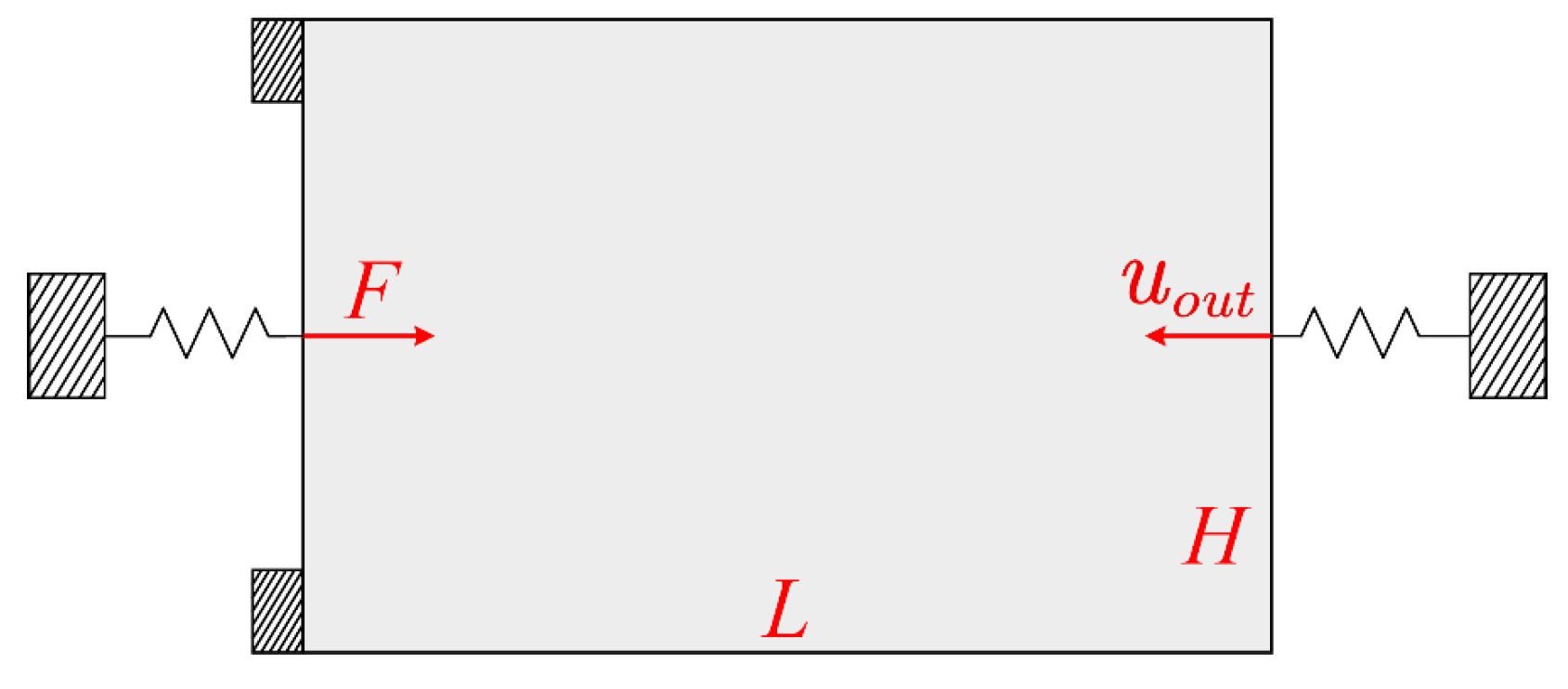
5.6. The Design of a Force Inventor
6. Concluding Remarks
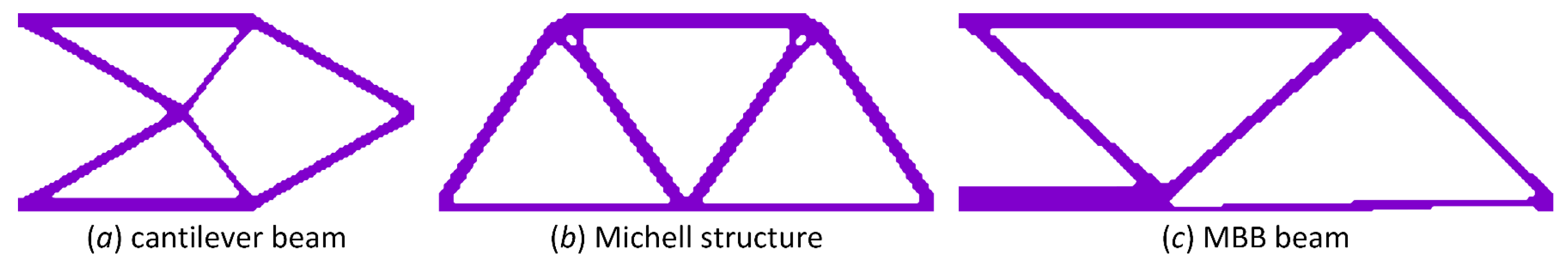
- IGA with higher numerical precision than the conventional FEM plays a significant role in optimization by maintaining the form of a full loading-transmission path in the topology.
- The extended DDF with the ersatz material model can be more beneficial by lowering the overestimation of the structural stiffness resulting from the material penalization model.
- The development of the extended DDF to unify the representations of binary and smooth designs can offer more benefits for optimization.
- In the ITO method with the ersatz material model, the threshold projection in the extended DDF can effectively support the generation of an appropriate topology.
Author Contributions
Funding
Institutional Review Board Statement
Informed Consent Statement
Data Availability Statement
Acknowledgments
Conflicts of Interest
References
- Bendsøe, M.P.; Sigmund, O. Topology Optimization: Theory, Methods and Applications; Springer Science & Business Media: Berlin/Heidelberg, Germany, 2003. [Google Scholar]
- Bendsøe, M.P.; Kikuchi, N. Generating Optimal Topologies in Structural Design Using a Homogenization Method. Comput. Methods Appl. Mech. Eng. 1988, 71, 197–224. [Google Scholar] [CrossRef]
- Zhou, M.; Rozvany, G.I.N. The COC Algorithm, Part II: Topological, Geometrical and Generalized Shape Optimization. Comput. Methods Appl. Mech. Eng. 1991, 89, 309–336. [Google Scholar] [CrossRef]
- Bendsøe, M.P.; Sigmund, O. Material Interpolation Schemes in Topology Optimization. Arch. Appl. Mech. 1999, 69, 635–654. [Google Scholar] [CrossRef]
- Xie, Y.M.; Steven, G.P. A Simple Evolutionary Procedure for Structural Optimization. Comput. Struct. 1993, 49, 885–969. [Google Scholar] [CrossRef]
- Huang, X.; Xie, Y.M. Bi-Directional Evolutionary Topology Optimization of Continuum Structures with One or Multiple Materials. Comput. Mech. 2009, 43, 393–401. [Google Scholar] [CrossRef]
- Sethian, J.A.; Wiegmann, A. Structural Boundary Design via Level Set and Immersed Interface Methods. J. Comput. Phys. 2000, 163, 489–528. [Google Scholar] [CrossRef]
- Wang, M.Y.; Wang, X.; Guo, D. A Level Set Method for Structural Topology Optimization. Comput. Methods Appl. Mech. Eng. 2003, 192, 227–246. [Google Scholar] [CrossRef]
- Allaire, G.; Jouve, F.; Toader, A.M. Structural Optimization Using Sensitivity Analysis and a Level-Set Method. J. Comput. Phys. 2004, 194, 363–393. [Google Scholar] [CrossRef] [Green Version]
- Guo, X.; Zhang, W.; Zhong, W. Doing Topology Optimization Explicitly and Geometrically—A Mew Moving Morphable Components Based Framework. J. Appl. Mech. 2014, 81, 081009. [Google Scholar] [CrossRef]
- Zhang, W.; Yang, W.; Zhou, J.; Li, D.; Guo, X. Structural Topology Optimization through Explicit Boundary Evolution. J. Appl. Mech. 2017, 84, 011011. [Google Scholar] [CrossRef]
- Gao, J.; Xue, H.; Gao, L.; Luo, Z. Topology Optimization for Auxetic Metamaterials Based on Isogeometric Analysis. Comput. Methods Appl. Mech. Eng. 2019, 352, 211–236. [Google Scholar] [CrossRef]
- Gao, J.; Luo, Z.; Li, H.; Gao, L. Topology Optimization for Multiscale Design of Porous Composites with Multi-Domain Microstructures. Comput. Methods Appl. Mech. Eng. 2019, 344, 451–476. [Google Scholar] [CrossRef]
- Zhang, Y.; Xiao, M.; Gao, L.; Gao, J.; Li, H. Multiscale Topology Optimization for Minimizing Frequency Responses of Cellular Composites with Connectable Graded Microstructures. Mech. Syst. Signal Process. 2020, 135, 106369. [Google Scholar] [CrossRef]
- Li, Q.; Sigmund, O.; Jensen, J.S.; Aage, N. Reduced-Order Methods for Dynamic Problems in Topology Optimization: A Comparative Study. Comput. Methods Appl. Mech. Eng. 2021, 387, 114149. [Google Scholar] [CrossRef]
- Chu, S.; Townsend, S.; Featherston, C.; Kim, H.A. Simultaneous Layout and Topology Optimization of Curved Stiffened Panels. AIAA J. 2021, 59, 2768–2783. [Google Scholar] [CrossRef]
- Chu, S.; Featherston, C.; Kim, H.A. Design of Stiffened Panels for Stress and Buckling via Topology Optimization. Struct. Multidiscip. Optim. 2021, 64, 3123–3146. [Google Scholar] [CrossRef]
- Xiao, M.; Liu, X.; Zhang, Y.; Gao, L.; Gao, J.; Chu, S. Design of Graded Lattice Sandwich Structures by Multiscale Topology Optimization. Comput. Methods Appl. Mech. Eng. 2021, 384, 113949. [Google Scholar] [CrossRef]
- Li, Q.; Xu, R.; Wu, Q.; Liu, S. Topology Optimization Design of Quasi-Periodic Cellular Structures Based on Erode–Dilate Operators. Comput. Methods Appl. Mech. Eng. 2021, 377, 113720. [Google Scholar] [CrossRef]
- Zhang, Y.; Zhang, L.; Ding, Z.; Gao, L.; Xiao, M.; Liao, W.-H. A Multiscale Topological Design Method of Geometrically Asymmetric Porous Sandwich Structures for Minimizing Dynamic Compliance. Mater. Des. 2022, 214, 110404. [Google Scholar] [CrossRef]
- Matsui, K.; Terada, K. Continuous Approximation of Material Distribution for Topology Optimization. Int. J. Numer. Methods Eng. 2004, 59, 1925–1944. [Google Scholar] [CrossRef]
- Guest, J.K.; Prévost, J.H.; Belytschko, T. Achieving Minimum Length Scale in Topology Optimization Using Nodal Design Variables and Projection Functions. Int. J. Numer. Methods Eng. 2004, 61, 238–254. [Google Scholar] [CrossRef]
- Rahmatalla, S.F.; Swan, C.C. A Q4/Q4 Continuum Structural Topology Optimization Implementation. Struct. Multidiscip. Optim. 2004, 27, 130–135. [Google Scholar] [CrossRef] [Green Version]
- Paulino, G.H.; Le, C.H. A Modified Q4/Q4 Element for Topology Optimization. Struct. Multidiscip. Optim. 2009, 37, 255–264. [Google Scholar] [CrossRef]
- Kang, Z.; Wang, Y. Structural Topology Optimization Based on Non-Local Shepard Interpolation of Density Field. Comput. Methods Appl. Mech. Eng. 2011, 200, 3515–3525. [Google Scholar] [CrossRef]
- Kang, Z.; Wang, Y. A Nodal Variable Method of Structural Topology Optimization Based on Shepard Interpolant. Int. J. Numer. Methods Eng. 2012, 90, 329–342. [Google Scholar] [CrossRef]
- Da, D.; Xia, L.; Li, G.; Huang, X. Evolutionary Topology Optimization of Continuum Structures with Smooth Boundary Representation. Struct. Multidiscip. Optim. 2018, 57, 2143–2159. [Google Scholar] [CrossRef]
- Andreasen, C.S.; Elingaard, M.O.; Aage, N. Level Set Topology and Shape Optimization by Density Methods Using Cut Elements with Length Scale Control. Struct. Multidiscip. Optim. 2020, 20, 685–707. [Google Scholar] [CrossRef]
- Huang, X. Smooth Topological Design of Structures Using the Floating Projection. Eng. Struct. 2020, 208, 110330. [Google Scholar] [CrossRef]
- Huang, X. On Smooth or 0/1 Designs of the Fixed-Mesh Element-Based Topology Optimization. Adv. Eng. Softw. 2021, 151, 102942. [Google Scholar] [CrossRef]
- Fu, Y.F.; Rolfe, B.; Chiu, L.N.S.; Wang, Y.; Huang, X.; Ghabraie, K. SEMDOT: Smooth-Edged Material Distribution for Optimizing Topology Algorithm. Adv. Eng. Softw. 2020, 150, 102921. [Google Scholar] [CrossRef]
- Berrut, J.-P.; Trefethen, L.N. Barycentric Lagrange Interpolation. SIAM Rev. 2004, 46, 501–517. [Google Scholar] [CrossRef] [Green Version]
- De Boor, C. A Practical Guide to Splines. Math. Comput. 1978, 27, 325. [Google Scholar]
- Piegl, L.; Tiller, W. The NURBS Book; Springer Science & Business Media: Berlin/Heidelberg, Germany, 2012. [Google Scholar]
- Hassani, B.; Khanzadi, M.; Tavakkoli, S.M. An Isogeometrical Approach to Structural Topology Optimization by Optimality Criteria. Struct. Multidiscip. Optim. 2012, 45, 223–233. [Google Scholar] [CrossRef]
- Qian, X. Topology Optimization in B-Spline Space. Comput. Methods Appl. Mech. Eng. 2013, 265, 15–35. [Google Scholar] [CrossRef]
- Liu, H.; Yang, D.; Hao, P.; Zhu, X. Isogeometric Analysis Based Topology Optimization Design with Global Stress Constraint. Comput. Methods Appl. Mech. Eng. 2018, 342, 625–652. [Google Scholar] [CrossRef]
- Gao, J.; Gao, L.; Luo, Z.; Li, P. Isogeometric Topology Optimization for Continuum Structures Using Density Distribution Function. Int. J. Numer. Methods Eng. 2019, 119, 991–1017. [Google Scholar] [CrossRef]
- Gao, J.; Luo, Z.; Xiao, M.; Gao, L.; Li, P. A NURBS-Based Multi-Material Interpolation (N-MMI) for Isogeometric Topology Optimization of Structures. Appl. Math. Model. 2020, 81, 818–843. [Google Scholar] [CrossRef]
- Hughes, T.J.R.; Cottrell, J.A.A.; Bazilevs, Y. Isogeometric Analysis: CAD, Finite Elements, NURBS, Exact Geometry and Mesh Refinement. Comput. Methods Appl. Mech. Eng. 2005, 194, 4135–4195. [Google Scholar] [CrossRef] [Green Version]
- Cottrell, J.A.; Hughes, T.J.R.; Bazilevs, Y. Isogeometric Analysis: Toward Integration of CAD and FEA; John Wiley & Sons: Hoboken, NJ, USA, 2009; ISBN 9780470748732. [Google Scholar]
- Kang, P.; Youn, S.K. Isogeometric Analysis of Topologically Complex Shell Structures. Finite Elem. Anal. Des. 2015, 99, 68–81. [Google Scholar] [CrossRef]
- Gu, J.; Yu, T.; Van Lich, L.; Nguyen, T.T.; Bui, T.Q. Adaptive Multi-Patch Isogeometric Analysis Based on Locally Refined B-Splines. Comput. Methods Appl. Mech. Eng. 2018, 339, 704–738. [Google Scholar] [CrossRef]
- Gu, J.; Yu, T.; Van Lich, L.; Nguyen, T.-T.; Tanaka, S.; Bui, T.Q. Multi-Inclusions Modeling by Adaptive XIGA Based on LR B-Splines and Multiple Level Sets. Finite Elem. Anal. Des. 2018, 148, 48–66. [Google Scholar] [CrossRef]
- Huynh, G.D.; Zhuang, X.; Bui, H.G.; Meschke, G.; Nguyen-Xuan, H. Elasto-Plastic Large Deformation Analysis of Multi-Patch Thin Shells by Isogeometric Approach. Finite Elem. Anal. Des. 2020, 173. [Google Scholar] [CrossRef]
- Wang, Y.; Benson, D.J. Isogeometric Analysis for Parameterized LSM-Based Structural Topology Optimization. Comput. Mech. 2016, 57, 19–35. [Google Scholar] [CrossRef]
- Jahangiry, H.A.; Tavakkoli, S.M. An Isogeometrical Approach to Structural Level Set Topology Optimization. Comput. Methods Appl. Mech. Eng. 2017, 319, 240–257. [Google Scholar] [CrossRef]
- Gao, J.; Xiao, M.; Zhou, M.; Gao, L. Isogeometric Topology and Shape Optimization for Composite Structures Using Level-Sets and Adaptive Gauss Quadrature. Compos. Struct. 2022, 285, 115263. [Google Scholar] [CrossRef]
- Xie, X.; Wang, S.; Xu, M.; Wang, Y. A New Isogeometric Topology Optimization Using Moving Morphable Components Based on R-Functions and Collocation Schemes. Comput. Methods Appl. Mech. Eng. 2018, 339, 61–90. [Google Scholar] [CrossRef]
- Zhang, W.; Li, D.; Kang, P.; Guo, X.; Youn, S.-K.K. Explicit Topology Optimization Using IGA-Based Moving Morphable Void (MMV) Approach. Comput. Methods Appl. Mech. Eng. 2020, 360, 112685. [Google Scholar] [CrossRef]
- Hou, W.; Gai, Y.; Zhu, X.; Wang, X.; Zhao, C.; Xu, L.; Jiang, K.; Hu, P. Explicit Isogeometric Topology Optimization Using Moving Morphable Components. Comput. Methods Appl. Mech. Eng. 2017, 326, 694–712. [Google Scholar] [CrossRef]
- Gao, J.; Xiao, M.; Zhang, Y.; Gao, L. A Comprehensive Review of Isogeometric Topology Optimization: Methods, Applications and Prospects. Chinese J. Mech. Eng. 2020, 33, 87. [Google Scholar] [CrossRef]
- Sigmund, O.; Maute, K. Topology Optimization Approaches. Struct. Multidiscip. Optim. 2013, 48, 1031–1055. [Google Scholar] [CrossRef]
- Andreassen, E.; Clausen, A.; Schevenels, M.; Lazarov, B.S.; Sigmund, O. Efficient Topology Optimization in MATLAB Using 88 Lines of Code. Struct. Multidiscip. Optim. 2011, 43, 1–16. [Google Scholar] [CrossRef] [Green Version]
- Sigmund, O. Morphology-Based Black and White Filters for Topology Optimization. Struct. Multidiscip. Optim. 2007, 33, 401–424. [Google Scholar] [CrossRef] [Green Version]
- Wang, F.; Lazarov, B.S.; Sigmund, O. On Projection Methods, Convergence and Robust Formulations in Topology Optimization. Struct. Multidiscip. Optim. 2011, 43, 767–784. [Google Scholar] [CrossRef]
- Xu, S.; Cai, Y.; Cheng, G. Volume Preserving Nonlinear Density Filter Based on Heaviside Functions. Struct. Multidiscip. Optim. 2010, 41, 495–505. [Google Scholar] [CrossRef]


| L | H | p | q | Control Points | IGA Elements | Vmax | |
|---|---|---|---|---|---|---|---|
| (a) | 10 | 5 | 1 | 1 | 161 × 81 | 160 × 80 | 0.2 |
| (b) | 10 | 4 | 1 | 1 | 151 × 61 | 150 × 60 | 0.2 |
| (c) | 12 | 4 | 1 | 1 | 181 × 61 | 180 × 60 | 0.2 |
| ITO with Ersatz Material Model | ITO with Material Penalization | |||||||
|---|---|---|---|---|---|---|---|---|
| Iter | Iter | |||||||
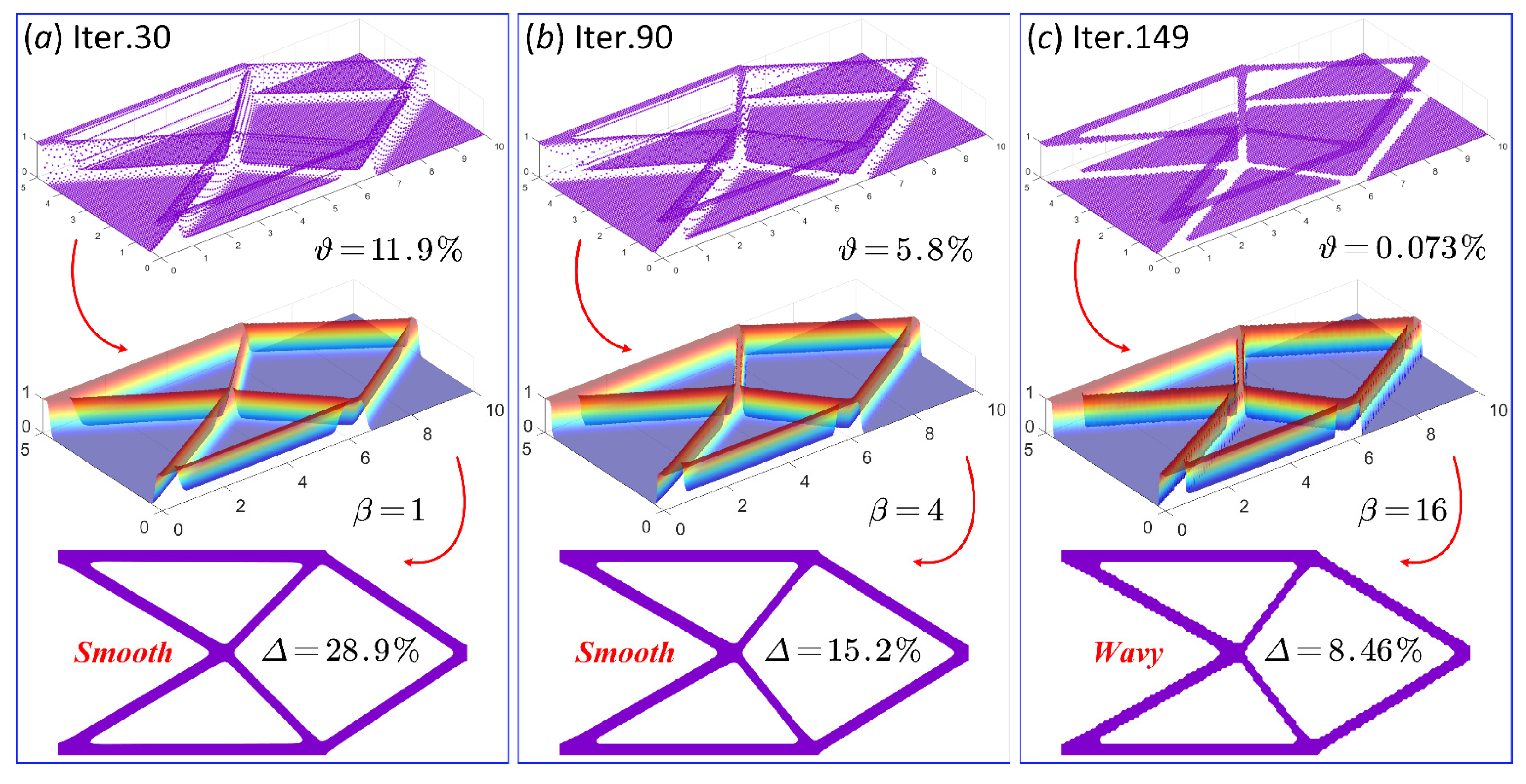
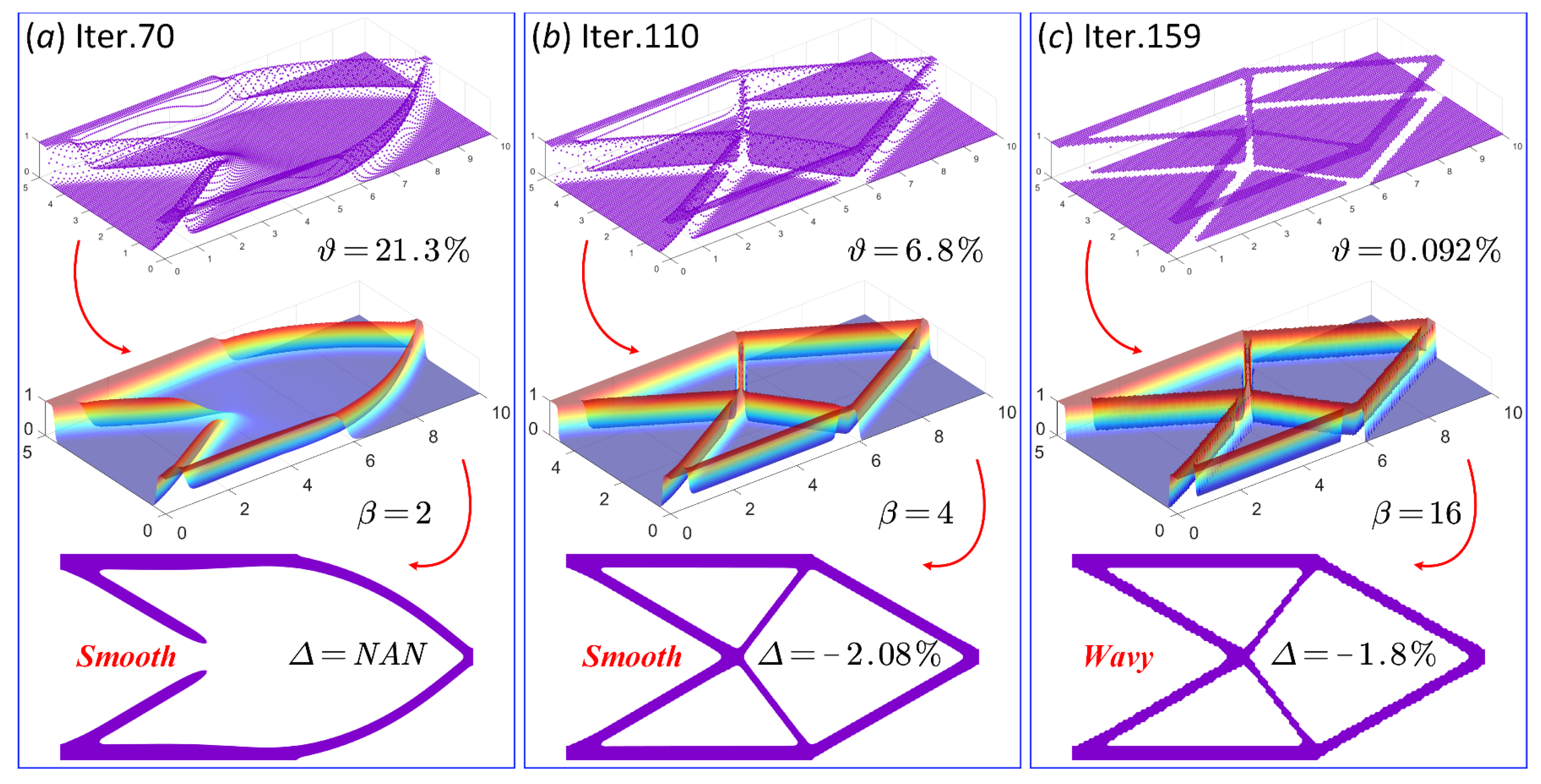
| (a) | 139.13 | 141.63 | −1.8% | 159 | 154.91 | 142.83 | 8.46% | 149 |
| (b) | 38.98 | 39.63 | −1.6% | 156 | 44.01 | 39.87 | 10.38% | 163 |
| (c) | 417.04 | 419.37 | −0.56% | 174 | 454.69 | 418.70 | 8.6% | 162 |
| p | q | r | Control Points | IGA Elements | Vmax | |
|---|---|---|---|---|---|---|
| (a) | 1 | 1 | 1 | 31 × 31 × 21 | 30 × 30 × 20 | 0.2 |
| (b) | 1 | 1 | 1 | 76 × 19 × 19 | 72 × 18 × 18 | 0.2 |
| (c) | 1 | 1 | 1 | 73 × 19 × 19 | 70 × 18 × 18 | 0.2 |
| L | H | p | q | Control Points | IGA Elements | Vmax | |
|---|---|---|---|---|---|---|---|
| (a) | 5 | 4 | 1 | 1 | 101 × 81 | 100 × 80 | 0.2 |
Publisher’s Note: MDPI stays neutral with regard to jurisdictional claims in published maps and institutional affiliations. |
© 2022 by the authors. Licensee MDPI, Basel, Switzerland. This article is an open access article distributed under the terms and conditions of the Creative Commons Attribution (CC BY) license (https://creativecommons.org/licenses/by/4.0/).
Share and Cite
Wu, X.; Zhang, Y.; Gao, L.; Gao, J. On the Indispensability of Isogeometric Analysis in Topology Optimization for Smooth or Binary Designs. Symmetry 2022, 14, 845. https://doi.org/10.3390/sym14050845
Wu X, Zhang Y, Gao L, Gao J. On the Indispensability of Isogeometric Analysis in Topology Optimization for Smooth or Binary Designs. Symmetry. 2022; 14(5):845. https://doi.org/10.3390/sym14050845
Chicago/Turabian StyleWu, Xiaomeng, Yan Zhang, Liang Gao, and Jie Gao. 2022. "On the Indispensability of Isogeometric Analysis in Topology Optimization for Smooth or Binary Designs" Symmetry 14, no. 5: 845. https://doi.org/10.3390/sym14050845
APA StyleWu, X., Zhang, Y., Gao, L., & Gao, J. (2022). On the Indispensability of Isogeometric Analysis in Topology Optimization for Smooth or Binary Designs. Symmetry, 14(5), 845. https://doi.org/10.3390/sym14050845