Ulam Stability of Fractional Hybrid Sequential Integro-Differential Equations with Existence and Uniqueness Theory

Abstract

In this paper, a variety of boundary value problems (BVPs) known as hybrid fractional sequential integro-differential equations (HFSIDs) with two point orders ($\mathfrak{p},\mathfrak{q}$) are investigated. The uniqueness and existence of the solution are discussed via Banach fixed-point theorems. Certain particular theorems associated with Hyers–Ulam and Hyers–Ulam–Rassias stability to the solution, as well as the uniqueness and existence of the solution of the BVPs are studied. The results are illustrated with some particular examples, and the numerical data are analyzed for confirmation of the results. The results obtained in this work are simple and can easily be applicable to physical systems. Furthermore, symmetry analysis of fractional differential equations and HFSIDs are also presented. This is due to the fact that the aforementioned analysis plays a significant role in both the optimization and qualitative theory of fractional differential equations.

1. Introduction

In a variety of scientific and engineering fields such as the electrodynamics of complex media, statistics, chemistry, biology, heat transfer analysis, hydro and thermo dynamics, several waves phenomena, fractal theory, physics, control theory, economics, image signals and processing, and bio-physics, various phenomena are modeled mathematically in the form of linear/nonlinear fractional ordinary differential equations/fractional partial differential equations (FODEs/FPDEs) [1,2]. Similarly, the concept of symmetry is a novel phenomenon in fractional calculus applied to investigate real-world problems, as well as used to study the correlation between applied and mathematical sciences [3,4,5,6], for example physics, fluid mechanics, dynamical systems, biology, control theory, entropy theory, and many areas of engineering [7,8,9]. Fractional differential equations can be used to more accurately describe some real-world issues in physics, mechanics, and other disciplines. Therefore, fractional-order differential equations have attracted much attention lately and are now a prominent subfield of nonlinear analysis. Fractional differential equations have been the subject of numerous monographs. Several researchers have recently conducted extensive studies on differential equations and inclusions with various boundary conditions. For more information and references, please see the subsequent part of the Introduction and the references therein.

The most helpful applications in fractional calculus are the Riemann–Liouville (R-L) and Caputo fractional derivatives. The Riesz fractional derivative linearly represents both the left fractional R-L derivative and the right fractional R-L derivative. The Caputo and the fractional R-L derivatives are relatively connected. It has been proven that, under the appropriate regularity assumptions, it is possible to convert the fractional R-L derivative into the Caputo fractional derivative [10,11]. In FPDEs, the time-fractional derivatives are usually defined by applying the Caputo fractional derivatives. The fundamental issue is that the initial conditions for the R-L method are necessary to comprise the R-L fractional derivative limit at time $t=0$, which has uncertain physical significance. It is worth mentioning that the foundation standards of the classical derivatives of the given functions at any time $t=0$ are the same for Caputo derivatives similar to integer-order differential equations [12,13].

Currently, hybrid fractional differential equations comprise one of the most extensive areas of interest in FPDEs, which mainly involves the fractional derivative of a hybrid unknown function that depends on the nonlinearity that appears in the given system [14,15]. A number of research articles [16,17] have presented various new findings on hybrid differential equations. For example, Miller and Ross [18,19] defined sequential derivatives in a monograph, a type of fractional derivative that combines the available derivative operators. Similarly, a relationship between the common R-L derivative and the fractional derivative of the sequential form was extensively studied in [20,21]. In addition, some academics have looked into hybrid fractional differential equations. A hybrid unknown function’s fractional derivative and the nonlinearity that depends on it are both present in this class of equations. In a number of papers [14,15,16,17], some recent findings on hybrid differential equations are presented.

The stability theory of FPDEs has obtained great consideration since Ulam gave the idea in 1940 and 1941. Since then, Rassias developed the Hyers–Ulam stability for both nonlinear and linear functions in 1982 and 1998. The Hyers–Ulam stability for linear DEs was first introduced in 1997 by Obloza [22,23,24,25]. Due to the inclusion of numerous vigorous systems as special instances, research of the HFSID equations has significant applications. The uniqueness and existence analysis for the solution of the standard hybrid differential equations of the first order with a leading form of perturbation were explored by Dhage and Lakshmikantham and Dhage and Jadhav, respectively, in [26,27]. Recently, Jamil et al. [28] discussed extensively the uniqueness and existence of the subsequent hybrid fractional sequential integro-differential equation:

$$\left\{\begin{array}{c}{}^{\mathfrak{c}}{\mathfrak{D}}^{\mathfrak{p}}\left[\frac{{}^{\mathfrak{c}}{\mathfrak{D}}^{\mathfrak{q}}\xi \left(t\right)-{\displaystyle \sum _{i=0}^m}{I}^{{\delta }_i}{h}_i(t,\xi \left(t\right))}{\mathrm{f}(t,\xi (t\left)\right)}\right]=g(t,\xi \left(t\right),I^{\gamma }\xi \left(t\right)),\forall t\in [0,1],\hfill \\ \xi \left(0\right)=0,{}^{\mathfrak{c}}{\mathfrak{D}}^{\mathfrak{q}}\xi \left(0\right)=0,\xi \left(1\right)=\Delta \xi \left(\eta \right),0<\Delta ,\eta <1.\hfill \end{array}\right.$$

(1)

Following the idea used for the existence and uniqueness in Equation (1), we use the following hybrid fractional sequential integro-differential (HFSID) equation with the two points orders ($\mathfrak{p},\mathfrak{q}$) with different boundary conditions as

$$\left\{\begin{array}{c}{}^{\mathfrak{c}}{\mathfrak{D}}^{\mathfrak{p}}\left[\frac{{}^{\mathfrak{c}}{\mathfrak{D}}^{\mathfrak{q}}\xi \left(t\right)-{\displaystyle \sum _{i=0}^m}{I}^{{\delta }_i}{h}_i(t,\xi \left(t\right))}{\mathrm{f}(t,\xi (t\left)\right)}\right]=g(t,\xi \left(t\right),I^{\gamma }\xi \left(t\right)),t\in [0,1],\hfill \\ \xi \left(0\right)=0,\xi \left(1\right)=b,b\in \mathfrak{R},{}^{\mathfrak{c}}{\mathfrak{D}}^{\mathfrak{q}},\xi \left(0\right)=0,\mathfrak{p}\in (0,1],\mathfrak{q}\in (1,2],\mathfrak{p}+\mathfrak{q}\in (2,3],\hfill \end{array}\right.$$

(2)

where ${}^{\mathfrak{c}}{\mathfrak{D}}^{\mathfrak{p}}$, ${}^{\mathfrak{c}}{\mathfrak{D}}^{\mathfrak{q}}$ indicates Caputo’s fractional operator of order $\mathfrak{p}$ and $\mathfrak{q}$. It should be noted that $0<\mathfrak{p}<2,0<\mathfrak{q}\le 2$. Further, the fractional R-L integral of order $\gamma$ is denoted by $I^{\gamma }$, and the fractional R-L sequential integral of order ${\delta }_i$ is denoted by $I^{{\delta }_i}$ for $i>0$ with $h_i(0,0)=0$. It should be further noted that the functions $h_i\in C([0,1]\times \mathbb{R},\mathbb{R})$, $\mathrm{f}\in C\left(\right[0,1]\times \mathbb{R},\mathbb{R}-\{0\left\}\right)$ and g$\in C([0,1]\times {\mathbb{R}}^2,\mathbb{R})$.

2. Preliminaries

Here, are some fundamental definitions of fractional calculus, as well as some theorems that guarantee the existence of the results from initial value problems.

Definition 1.

The following formula defines the fractional R-L integral for $\mathfrak{p}>0$ for a continuous function $\xi :(0,\infty )\to \mathbb{R}$.

$$I^{\mathfrak{p}}\xi \left(t\right)=\frac{1}{\Gamma \left(\mathfrak{p}\right)}{\int }_0^t{(t-\mathrm{s})}^{\mathfrak{p}-1}\xi \left(\mathrm{s}\right)d\mathrm{s}.$$

assuming that the above integral is well defined on the set of real numbers.

Definition 2.

The fractional R-L derivative for $\mathfrak{p}>0$ of a continuous function ξ defined above is given by

$$\begin{array}{c}\hfill {\mathfrak{D}}^{\mathfrak{p}}\xi \left(t\right)=\frac{1}{\Gamma (n-\mathfrak{p})}\frac{d^n}{d{t}^n}{\int }_0^t{(t-\mathrm{s})}^{n-\mathfrak{p}-1}\xi \left(\mathrm{s}\right)d\mathrm{s},\forall \mathfrak{p}\in (n-1,n].\end{array}$$

Definition 3.

The function $\xi :(0,\infty )\to \mathbb{R}$ defines Caputo’s fractional derivative for $\mathfrak{p}>0$ of a function $\xi \left(t\right)$ as

$${\mathfrak{D}}^{\mathfrak{p}}\xi \left(t\right)=\frac{1}{\Gamma (n-\mathfrak{p})}{\int }_0^t{(t-\mathrm{s})}^{n-\mathfrak{p}-1}{\xi }^n\left(\mathrm{s}\right)d\mathrm{s},\forall \mathfrak{p}\in (n-1,n],$$

where the integral on the right-hand side is distinctly defined on the interval $(0,\infty )$ and $n=\left[\mathfrak{p}\right]+1$. Here, $\left[\mathfrak{p}\right]$ is a bracket function, which signifies the integer component of order $\mathfrak{p}$.

Proposition 1.

If $\beta ,\mathfrak{q}>0$, and $\xi \left(t\right)$ are functions, then $I^{\beta }\left[I^{\mathfrak{q}}\xi \left(t\right)\right]=I^{\beta }+\mathfrak{q}\xi \left(t\right)$ is the property of the semi-group for the fractional R-L integrals of order β and $\mathfrak{q}$, respectively.

Theorem 1.

Arzelà–Ascoli Theorem

A subset S of the space of continues functions $C\left(X\right)$ is compact iff S is closed, bounded, and equi-continuous.

Lemma 1

([29]).For the function $\xi \in L(0,T)\cap C(0,T)$, the solution $\xi \left(t\right)$ of the fractional Caputo’s differential equation of the form:

$$\begin{array}{c}\hfill {}^{\mathfrak{c}}{\mathfrak{D}}^{\mathfrak{q}}\xi \left(t\right)=g\left(t\right),\mathfrak{q}\in (n-1,n],\end{array}$$

is presented by

$$\begin{array}{c}\hfill \xi \left(t\right)=I^{\mathfrak{q}}g\left(t\right)+k_0+k_{1}t+\cdots +k_{n-1}t=I^{\mathfrak{q}}g\left(t\right)+\sum _{i=0}^{n-1}{k}_i{t}^i=\xi \left(t\right),\end{array}$$

Here, we establish $\parallel ·\parallel$ and a multiplication $(\times )$ in $E=C\left(\right[0,1],\mathbb{R})$ (a Banach space) by $\left|\right|\xi \left|\right|=\underset{t\in J}{sup}\left|\xi \left(t\right)\right|$ and $\left(\xi \mathfrak{v}\right)\left(t\right)=\xi \left(t\right)\mathfrak{v}\left(t\right)$, for all $t\in J=[0,1]$. Therefore, if E is a Banach space, then the multiplication and norm mentioned above should be satisfied.

Lemma 2

([26]).Suppose $S\subseteq E$ is closed, bounded, and convex. Further suppose that two operators $\mathcal{A}$ and $\mathcal{B}$ such that $\mathcal{A}:E\to E$ and $\mathcal{B}:S\to E$ satisfy the following conditions:

(c₁) 

The operator $\mathcal{A}$ is contractive;

(c₂) 

The operator $\mathcal{B}$ is compact;

(c₃) 

The function ξ is of the form $\xi =\mathcal{A}\xi +\mathcal{B}\zeta$ such that, for all $\zeta \in S$, it implies that $\xi \in S$.

Then, the solution for the operator equation $\xi =\mathcal{A}\xi +\mathcal{B}\zeta$ exists.

To discuss the Ulam stability, let us examine the equation of the form:

$${\mathfrak{D}}^{\mathfrak{p}}\xi \left(t\right)=g(t,\xi \left(t\right)),\forall t\in J=[0,T],n-1<\mathfrak{p}\le n,$$

(3)

Definition 4

([30]).For any constant $k>0$ such that the inequality below has a solution for any arbitrary $g\in C\left(\right[0,T],\mathbb{R})$ and $ϵ>0$, then Equation (3) is supposed to be Hyers–Ulam stable.

$$|D^{\mathfrak{p}}g\left(t\right)-g(t,g\left(t\right))|\le \in ,\forall t\in J,$$

(4)

∃ a solution $\xi \left(t\right)$ of Equation (3) such that

$$\left|g\right(t)-\xi (t\left)\right|\le \in k,\mathit{for}\mathit{all}t\in J.$$

(5)

Definition 5

([30]).For any constant $k_{\varphi ,g}$ such that the solution of the subsequent inequality holds for any arbitrary $ϵ>0$, then Equation (3) is said to be Hyers–Ulam–Rassias stable for

$$|{\mathfrak{D}}^{\mathfrak{p}}g\left(t\right)-g(t,g\left(t\right))|\le \in \varphi \left(t\right),\mathit{for}\mathit{all}t\in J,$$

(6)

∃ solution $\xi \left(t\right)$ of Equation (3) satisfying

$$|g\left(t\right)-\xi \left(t\right)|\le \in k_{\varphi ,g}\varphi \left(t\right),\mathit{for}\mathit{all}t\in J=[0,T].$$

(7)

Remark 1

([30]).For a function $\Phi \in C\left(\right[0,T],\mathbb{R})$ (relies only on element $y\in C\left(\right[0,T],\mathbb{R}]$) so that:

• :$|\Phi (t\left)\right|\le \in ,\mathit{for}\mathit{all}t\in [0,T]$;
• :${\mathfrak{D}}^{\mathfrak{p}}y\left(t\right)=g(t,y\left(t\right))+\Phi \left(t\right),\mathit{for}\mathit{all}t\in J=[0,T]$.

then$g\in C\left(\right[0,T],\mathbb{R})$is a solution of Equation (4).

3. Symmetry Analysis of Fractional Differential Equations

Consider an independent variable $\xi \in \mathcal{R}$, $t>0$ and the independent function $u(t,\xi )$. The partial-order derivatives are denoted by ${\partial }_{\xi }^{i}u$ for $i=1,2,\cdots ,s$, and ${}^c{D}_t^{\alpha }u$ is the Caputo fractional derivative of order $\alpha$. Consider a general fractional partial differential equation of the form

$$F(\xi ,t,u{,}^c{D}_t^{\alpha }u,{\partial }_{\xi }u,{\partial }_{\xi }^{2}u,\cdots ,{\partial }_{\xi }^{s}u)=0,0<\alpha \le 1,$$

then the one-parameter Lie-symmetry method is given in the following transformation:

$$\begin{array}{cc}\hfill & \overline{t}=t+ϵ\tau (t,\xi ,u)+\mathcal{O}{ϵ}^2,\hfill \\ \hfill & \overline{\xi }=\xi +ϵ\xi (t,\xi ,u)+\mathcal{O}{ϵ}^2,\hfill \\ \hfill & \overline{u}=u+ϵ\eta (t,\xi ,u)+\mathcal{O}{ϵ}^2.\hfill \end{array}$$

Here, $\zeta ,{\tau }^{\prime },\eta$ are the infinitesimals such that $\zeta =\frac{d\overline{\xi }}{d\overline{ϵ}}{|}_{ϵ=0}$, ${\tau }^{\prime }=\frac{d\overline{\tau }}{d\overline{ϵ}}{|}_{ϵ=0}$, and $\eta =\frac{d\overline{u}}{d\overline{ϵ}}{|}_{ϵ=0}$.

3.1. Symmetry Analysis of Time-Fractional Boundary Value Problems

In this subsection, we study the symmetry analysis of the initial and boundary value problems in the Caputo sense. Consider the following fractional diffusion equation in Caputo’s form as

$${}^c{D}_{\tau }^{\alpha }u=\frac{d}{d\xi }\left(u^p\frac{du}{d\xi }\right),p\ne 0,0<\alpha \le 0,$$

with the initial and boundary conditions of the form

$$u(\tau ,0)=a\left(\tau \right),\mathrm{for}\tau >0,\mathrm{and}u(0,\xi )=b\left(\xi \right),\mathrm{for}\xi >0.$$

The symmetries for this equation were derived by Gazizov, Kasatkin, and Lukashchuk in [31], which we can use as an infinitesimal generator as

$$X=\left(c_1+\frac{\alpha \xi c_2}{2}+p{c}_3\xi \right)\frac{\partial }{\partial \xi }+t{c}_2\frac{\partial }{\partial t}+2u{c}_3\frac{\partial }{\partial u}.$$

(8)

where $c_1,c_2,c_3$ are arbitrary constant.

3.2. Symmetry Analysis of HFSID

In this section of the research, we look at the IBVPs one-parameter Lie symmetry analysis with Caputo fractional derivative. We know that it can explain actual processes in terms of natural processes. If the initial and boundary conditions for the HFSID are of the form:

$$\left\{\begin{array}{c}{}^{\mathfrak{c}}{\mathfrak{D}}^{\mathfrak{p}}\left[\frac{{}^{\mathfrak{c}}{\mathfrak{D}}^{\mathfrak{q}}\xi \left(t\right)-{\displaystyle \sum _{i=0}^m}{I}^{{\delta }_i}{h}_i(t,\xi \left(t\right))}{F(t,u(\xi ,t\left)\right)}\right]=G(t,\xi \left(t\right),I^{\gamma }\xi \left(t\right)),t\in [0,1],\hfill \\ \xi \left(0\right)=0,{}^{\mathfrak{c}}{\mathfrak{D}}^{\mathfrak{q}},\xi \left(0\right)=0,\hfill \end{array}\right.$$

(9)

where F and G are some known functions, then we follow the following definition.

Definition 6.

We say that the symmetry (8) admits Equation (9) with the boundary condition if:

• $X^{\left(k\right)}{D}^{\mathfrak{p}}$$\left({}^{\mathfrak{c}}{\mathfrak{D}}^{\mathfrak{q}}\xi \left(t\right)-G(t,\xi \left(t\right),I^{\gamma }\xi \left(t\right))\right)$ whenever $D^{\mathfrak{p}}$$\left({\mathfrak{D}}^{\mathfrak{q}}\xi \left(t\right)=G(t,\xi \left(t\right),I^{\gamma }\xi \left(t\right))\right)$;
• $X^{\left(c\right)}\left({}^c{D}^{\mathfrak{p}}\left({}^{\mathfrak{c}}{\mathfrak{D}}^{\mathfrak{q}}\xi \left(0\right)\right)\right)=0,$ whenever ${}^c{D}^{\mathfrak{p}}\left({}^{\mathfrak{c}}{\mathfrak{D}}^{\mathfrak{q}}\xi \left(0\right)\right)=0$;
• $X^{(k-1)}{D}^{\mathfrak{p}}\left({}^{\mathfrak{c}}{\mathfrak{D}}^{\mathfrak{q}}\xi \left(0\right)\right)=0,$ whenever ${}^c{D}^{\mathfrak{p}}\left({}^{\mathfrak{c}}{\mathfrak{D}}^{\mathfrak{q}}\xi \left(0\right)\right)=0$.

Definition 7.

The solution u = v(x, t) of Equation (9) is an invariant solution, resulting under the symmetry of Section 3 with infinitesimal generator (8) if and only if:

• u= v(x, t) satisfies Equation (sym1);
• u = v(x, t) is an invariance surface under X.

The following theorem will help for the symmetry of the HFSID equation.

Theorem 2.

u(x,t) = v(x,t) is an invariant solution of Equation (9) if and only if the function v(x,t) under the generator (8) allows the condition:

$$\eta (x,t,v(x,t))-\zeta (x,t,v(x,t))-\tau (x,t,v(x,t))D^{\mathfrak{1}-\mathfrak{p}}\left({\mathfrak{D}}^{\mathfrak{1}-\mathfrak{q}}\xi \left(t\right)G(t,\xi \left(t\right),I^{\gamma }\xi \left(t\right))\right)=0.$$

(10)

Proof. 

As the solution u = v(x,t) is invariant and admits the condition X(u − v(x,t)), then with the help of Definitions 6 and 7, we have

$$\begin{array}{cc}\hfill 0=X(u-v(\xi ,t\left)\right)& =\left(\left(c_1+\frac{\alpha \xi c_2}{2}+p{c}_3\xi \right)\frac{\partial }{\partial \xi }+t{c}_2\frac{\partial }{\partial t}+2u{c}_3\frac{\partial }{\partial u}\right)(u-v(x,t))\hfill \\ & =c_1\frac{\partial (u-v(\xi ,t\left)\right)}{\partial \xi }+\frac{\alpha \xi c_2}{2}\frac{\partial (u-v(\xi ,t\left)\right)}{\partial \xi }+p{c}_3\xi \frac{\partial (u-v(\xi ,t\left)\right)}{\partial \xi }\hfill \\ & +t{c}_1\frac{\partial (u-v(\xi ,t\left)\right)}{\partial t}+2u{c}_3\frac{\partial (u-v(\xi ,t\left)\right)}{\partial u},\hfill \end{array}$$

(11)

since $u=v(\xi ,t)$ so that $u_t=\frac{\partial u}{\partial t}$ and in Caputo’s form $u_t={}^c{D}^{\mathfrak{1}-\mathfrak{p}}\left({\mathfrak{D}}^{\mathfrak{1}-\mathfrak{q}}\xi \left(t\right)G(t,u\left(t\right),I^{\gamma }\xi \left(t\right))\right),$ finally we obtain:

$$\eta (\xi ,t,v(\xi ,t))-\zeta (\xi ,t,v(\xi ,t))-\tau (\xi ,t,v(\xi ,t))D^{\mathfrak{1}-\mathfrak{p}}\left({\mathfrak{D}}^{\mathfrak{1}-\mathfrak{q}}\xi \left(t\right)G(t,\xi \left(t\right),I^{\gamma }\xi \left(t\right))\right),$$

(12)

and this completes the proof. □

In the next section, we discuss the existence and uniqueness solution of Equation (2).

4. Solution and Existence of HFSID

This section examines the BVP for the HFSID in the form of (2). Using the concepts mentioned above and the findings covered in the previous section, we first derive the solution of the BVP (2) before going to the existence theory. Our solution is based on the following lemma.

Lemma 3.

If $0<\mathfrak{p}\le 1,1<\mathfrak{q}\le 2$, and $\gamma >0$ are satisfied by the functions $g_i,h_i$, and ${\mathrm{f}}_i$, then the BVP (2) has a unique solution provided by

$$\begin{array}{ccc}\hfill \xi \left(t\right)& =& {\int }_0^t\frac{{(t-\mathrm{s})}^{\mathfrak{q}-1}\mathrm{f}(\mathrm{s},\xi \left(\mathrm{s}\right))}{\Gamma \left(\mathfrak{q}\right)}{\int }_0^s\frac{{(\mathrm{s}-\mu )}^{\mathfrak{p}-1}g(\mu ,\xi \left(\mu \right),I^{\gamma }\xi \left(\mu \right))}{\Gamma \left(\mathfrak{p}\right)}d\mu d\mathrm{s}+[b+\sum _{i=1}^m{I}^{{\delta }_i+\mathfrak{q}}{h}_i(1,\xi \left(1\right))\hfill \\ & & -{\int }_0^1\frac{{(t-s\mathrm{s})}^{\mathfrak{q}-1}\mathrm{f}(\mathrm{s},\xi \left(\mathrm{s}\right))}{\Gamma \left(\mathfrak{q}\right)}{\int }_0^1\frac{{(1-\mathrm{s})}^{\mathfrak{p}-1}g(\mathrm{s},\xi \left(\mathrm{s}\right)}{\Gamma \left(\mathfrak{p}\right)},I^{\gamma }\xi \left(s\right)\left)d\mathrm{s}\right]t+\sum _{i=1}^m{I}^{{\delta }_i+\mathfrak{q}}{h}_i(t,\xi \left(t\right)),\hfill \end{array}$$

(13)

where

$$\begin{array}{c}\hfill I^{{\delta }_i+\mathfrak{q}}{h}_i(t,\xi \left(t\right))={\int }_0^t\frac{{(t-\mathrm{s})}^{{\delta }_i+\mathfrak{q}-1}}{\Gamma ({\delta }_i+\mathfrak{q})}{h}_i(\mathrm{s},\xi \left(\mathrm{s}\right))d\mathrm{s},\\ \hfill I^{{\delta }_i+\mathfrak{q}}{h}_i(1,\xi \left(1\right))={\int }_0^1\frac{{(1-\mathrm{s})}^{{\delta }_i+\mathfrak{q}-1}}{\Gamma ({\delta }_i+\mathfrak{q})}{h}_i(\mathrm{s},\xi \left(\mathrm{s}\right))d\mathrm{s}.\end{array}$$

Proof. 

Using the R-L fractional integral operator $\mathfrak{p}$ with the use of Lemma 1, the HFSID Equation (2) presumably obtained in the form:

$$\frac{{}^{\mathfrak{c}}{\mathfrak{D}}^{\mathfrak{q}}\xi \left(t\right)-{\displaystyle \sum _{i=1}^m}{I}^{{\delta }_i}{h}_i(t,\xi \left(t\right))}{\mathrm{f}(t,\xi (t\left)\right)}=I^{\mathfrak{p}}g(t,\xi \left(t\right),I^{\gamma }\xi \left(t\right))+k_0,$$

(14)

with the use of the subsidiary conditions $\xi \left(0\right)=0$, ${\mathfrak{D}}^{\mathfrak{q}}\xi \left(0\right)=0$, we have $h_i(0,0)=0$ and $k_0=0$. Thus, for $f(0,0)\ne 0$, Equation (14) takes the form:

$${\mathfrak{D}}^{\mathfrak{q}}\xi \left(t\right)=\sum _{i=1}^m{I}^{{\delta }_i}{h}_i(t,\xi \left(t\right))+\mathrm{f}(t,\xi \left(t\right)){\int }_0^t\frac{{(t-s)}^{\mathfrak{p}-1}g(s,\xi \left(s\right),I^{\gamma }\xi \left(s\right))}{\Gamma \left(\mathfrak{p}\right)}ds.$$

(15)

Next, we use the R-L fractional integral operator $\mathfrak{q}$ combined with Proposition 1 and Lemma 1 so that Equation (15) takes the form:

$$\xi \left(t\right)={\int }_0^t\frac{{(t-s)}^{\mathfrak{q}-1}\mathrm{f}(s,\xi \left(s\right))}{\Gamma \left(\mathfrak{q}\right)}{\int }_0^s\frac{{(s-\mu )}^{\mathfrak{p}-1}g(\mu ,\xi \left(\mu \right),I^{\gamma }\xi \left(\mu \right))}{\Gamma \left(\mathfrak{p}\right)}d\mu ds+\sum _{i=1}^m{I}^{{\delta }_i+\mathfrak{q}}{h}_i(t,\xi \left(t\right))+k_1+k_{2}t,$$

(16)

and by the application of the initial and boundary conditions of Equations (2) to (16), we have

$$k_1=0,k_2=b-\left[{\int }_0^1\frac{{(t-s)}^{\mathfrak{q}-1}\mathrm{f}(s,\xi \left(s\right))}{\Gamma \left(\mathfrak{q}\right)}·{\int }_0^1\frac{{(s-\mu )}^{\mathfrak{p}-1}g(s,\xi \left(s\right),I^{\gamma }\xi \left(s\right))}{\Gamma \left(\mathfrak{p}\right)}d\mu ds+\sum _{i=1}^m{I}^{{\delta }_i+\mathfrak{q}}{h}_i(1,\xi \left(1\right))\right]$$

After the inclusion of $k_2$, Equation (16) takes the form:

$$\begin{array}{ccc}\hfill \xi \left(t\right)& =& \frac{1}{\Gamma \left(\mathfrak{q}\right)}{\int }_0^t{(t-s)}^{\mathfrak{q}-1}\mathrm{f}(s,\xi \left(s\right))\frac{1}{\Gamma \left(\mathfrak{p}\right)}{\int }_0^s{(s-\mu )}^{\mathfrak{p}-1}g(\mu ,\xi \left(\mu \right),I^{\gamma }\xi \left(\mu \right))d\mu ds+\sum _{i=1}^m{I}^{{\delta }_i+\mathfrak{q}}{h}_i(t,\xi \left(t\right))\hfill \\ & & +t\left[b-{\int }_0^1\frac{{(t-s)}^{\mathfrak{q}-1}\mathrm{f}(s,\xi \left(s\right))}{\Gamma \left(\mathfrak{q}\right)}·{\int }_0^1\frac{{(1-s)}^{\mathfrak{p}-1}g(s,\xi \left(s\right),I^{\gamma }\xi \left(s\right))}{\Gamma \left(\mathfrak{p}\right)}ds+\sum _{i=1}^m{I}^{{\delta }_i+\mathfrak{q}}{h}_i(1,\xi \left(1\right))\right].\hfill \end{array}$$

(17)

This gives the unique solution of Equation (2). Hence, it is proven. □

The following suppositions are taken into consideration to obtain a result for the existence.

Theorem 3.

• ${\mathcal{A}}_1:$ The continuous functions $\mathrm{f}$, g are defined as $\mathrm{f}:[0,1]\times \mathbb{R}\to \mathbb{R}-\left\{0\right\}$ and $g:[0,1]\times {\mathbb{R}}^2\to \mathbb{R}$. Further, suppose that $h_i$ has positive functions $\varphi \left(t\right)$, $\chi \left(t\right)$, and ${\theta }_i\left(t\right)$, respectively, with bounds $\parallel \varphi \parallel$, $\parallel \chi \parallel$, and $\parallel {\theta }_i\parallel$. These positive functions are restricted as

  $$\begin{array}{ccc}\hfill \left|\mathrm{f}\right(t,\xi )-\mathrm{f}(t,\zeta |& \le & \varphi |\xi -\zeta |,\hfill \\ \hfill \left|g(t,\xi ,\overline{\xi })-g(t,\zeta ,\overline{\zeta }\right|& \le & \chi \left(\right|\xi -\zeta |+|\overline{\xi }-\overline{\zeta }\left|\right),\forall t\in [0,1]\mathrm{a}nd\xi ,\zeta \in \mathbb{R}.\hfill \end{array}$$
• ${\mathcal{A}}_2:$

  $$\begin{array}{ccc}\hfill \left|\mathrm{f}\right(t,\xi \left)\right|& \le & \xi \left(t\right),forall(t,\xi )\in [0,1]\times \mathbb{R},\xi \in C([0,1],{\mathbb{R}}_{+}),\hfill \\ \hfill \left|g\right(t,\xi ,\zeta \left)\right|& \le & \zeta ,forall(t,\xi ,\zeta )\in [0,1]\times \mathbb{R}\times \mathbb{R},\zeta \in C\left([0,1]R_{+}\right),\hfill \\ \hfill |h_i(t,\xi )|& \le & {\theta }_i,forall(t,\xi )\in [0,1]\times \mathbb{R},{\theta }_i\in C([0,1],{\mathbb{R}}_{+}).\hfill \end{array}$$
• ${\mathcal{A}}_3:$ For the real number $r>0$, we can derive

  $$\left[\sum _{i=1}^m\frac{\parallel {\varphi }_i\parallel }{\Gamma (1+{\delta }_i+\mathfrak{q})}\left(T^{{\delta }_i+\mathfrak{q}}+1\right)+\frac{T^{\mathfrak{p}+\mathfrak{q}}}{\Gamma (\mathfrak{q}+1)\Gamma (\mathfrak{p}+1)}\parallel \xi \parallel \parallel \zeta \parallel \right]\le r,$$

  and

  $$\left[\frac{T^{\mathfrak{p}}}{\Gamma (\mathfrak{p}+1)}\parallel \zeta \parallel \parallel \Theta \parallel +\parallel \chi \parallel \parallel \xi \parallel \left(\frac{T^{\mathfrak{p}}}{\Gamma (\mathfrak{p}+1)}+\frac{T^{\mathfrak{p}+\gamma }}{\Gamma (\gamma +\mathfrak{p}+1)}\right)\right]\left(\frac{T^{\mathfrak{q}}}{\Gamma (\mathfrak{q}+1)}-\frac{t}{\Gamma (\mathfrak{q}+1)}\right)<1.$$

  (18)

This shows that the BVP (2) has at least one solution on $J=[0,1]$.

The generalized Krasnoselikii fixed-point theorem by Dhage presented in [26] is the foundation for our primary existence conclusion, which is stated in Lemma 2.

Theorem 4.

Suppose the assumptions ${\mathcal{A}}_1-{\mathcal{A}}_3$ hold, then ∃ at least one solution in the interval $[0,1]$ of the BVP (2).

Proof. 

To prove our results, first, we set the bounds $\underset{t\in [0,1]}{sup}\left|\varphi \left(t\right)\right|=\parallel {\varphi }_i\parallel ,\underset{t\in [0,1]}{sup}\left|\xi \left(t\right)\right|=\parallel \xi \parallel ,\underset{t\in [0,1]}{sup}|{\Theta }_i\left(t\right)|=\parallel \Theta \parallel ,\underset{t\in [0,1]}{sup}\left|\zeta \right|=\parallel \zeta \parallel ,\underset{t\in [0,1]}{sup}\left|\chi \left(t\right)\right|=\parallel \chi \parallel$, for i = 1, 2,..., m.

Consider a Banach space $E=C\left(\right[0,1],\mathbb{R})$, and let $S\subseteq E$, where $S=\{\xi \in E:\parallel \xi \parallel \le \mathbb{R}\}$, then obviously, S is closed, bounded, and convex. Further, consider two operators $\mathcal{D}:E⟶E$ and $\mathcal{C}:E⟶E$, such that

$$\mathcal{C}\xi \left(t\right)={\int }_0^t\frac{{(t-s)}^{\mathfrak{p}-1}g(s,\xi \left(s\right))}{\Gamma \left(\mathfrak{p}\right)},I^{\gamma }\xi \left(t\right))ds,\mathrm{a}nd\mathcal{D}\xi \left(t\right)=\mathrm{f}(t,\xi \left(t\right)).$$

Using the assumptions $\left({\mathcal{A}}_1\right)$ and $\left({\mathcal{A}}_2\right)$ and the maximum in the interval $[0,1]$ gives

$$\begin{array}{ccc}\hfill \parallel \mathcal{C}\xi \left(t\right)-\mathcal{C}\zeta \left(t\right)\parallel & \le & \frac{\parallel \chi \parallel }{\Gamma (\mathfrak{p}+1)}\left(1+\frac{1}{\Gamma (\gamma +1)}\right)\parallel \xi -\zeta \parallel ,\hfill \\ \hfill \parallel \mathcal{D}\xi \left(t\right)-\mathcal{D}\zeta \left(t\right)\parallel & \le & \parallel \varphi \parallel \parallel \xi -\zeta \parallel ,\hfill \\ \hfill \parallel \mathcal{C}\xi \left(t\right)\parallel & \le & \frac{\parallel \chi \parallel }{\Gamma (\mathfrak{p}+1)}\hfill \\ \hfill \parallel \mathcal{D}\xi \left(t\right)\parallel & \le & \parallel \xi \parallel .\hfill \end{array}$$

Next, consider $\mathcal{A}:\mathcal{E}⟶\mathcal{E}$ and $\mathcal{B}:S⟶\mathcal{E}$, such that

$$\begin{array}{ccc}\hfill \mathcal{A}\xi \left(t\right)& =& {\int }_0^t\frac{{(t-s)}^{\mathfrak{q}-1}\mathcal{D}\xi \left(s\right)\mathcal{C}\xi \left(s\right)}{\Gamma \left(\mathfrak{q}\right)}ds+t\left[b-{\int }_0^1\frac{{(1-s)}^{\mathfrak{q}-1}\mathcal{D}\xi \left(s\right)\mathcal{C}\xi \left(s\right)}{\Gamma \left(\mathfrak{q}\right)}ds\right],\hfill \end{array}$$

(19)

and

$$\begin{array}{ccc}\hfill \mathcal{B}\xi \left(t\right)& =& \sum _{i=1}^m{\int }_0^t\frac{{(t-s)}^{{\delta }_i+\mathfrak{q}-1}{h}_i(s,\xi \left(s\right))}{\Gamma ({\delta }_i+\mathfrak{q})}ds+\sum _{i=1}^m{\int }_0^1\frac{{(1-s)}^{{\delta }_i+\mathfrak{q}-1}{h}_i(s,\xi \left(s\right))}{\Gamma ({\delta }_i+\mathfrak{q})}ds,\hfill \end{array}$$

(20)

then the integral in Equation (17) will take the subsequent conformation:

$$\xi \left(t\right)=\mathcal{A}\xi \left(t\right)+\mathcal{B}\xi \left(t\right),\forall t\in J[0,1].$$

(21)

In the subsequent operations, we present that the two operators $\mathcal{A}$ and $\mathcal{B}$ hold the entire conditions of Lemma 2.

Step 1. To show that the operator $\mathcal{A}$ is contractive, we consider two functions $\xi \left(t\right)$ and $\zeta \left(t\right)$ in the subspace S, then

$$\begin{array}{ccc}\hfill |\mathcal{A}\xi -\mathcal{A}\zeta |& \le & \frac{1}{\Gamma \left(\mathfrak{q}\right)}{\int }_0^t{(t-\mathrm{s})}^{\mathfrak{q}-1}|\mathfrak{D}\xi \left(\mathrm{s}\right)\mathcal{C}\xi \left(\mathrm{s}\right)-\mathfrak{D}\zeta \left(\mathrm{s}\right)\mathcal{C}\zeta \left(\mathrm{s}\right)|d\mathrm{s}\hfill \\ & -& \frac{t}{\Gamma \left(\mathfrak{q}\right)}{\int }_0^1{(1-\mathrm{s})}^{\mathfrak{q}-1}|\mathfrak{D}\xi \left(\mathrm{s}\right)\mathcal{C}\xi \left(\mathrm{s}\right)-\mathfrak{D}\zeta \left(\mathrm{s}\right)\mathcal{C}\zeta \left(\mathrm{s}\right)|d\mathrm{s}\hfill \\ & \le & \frac{1}{\Gamma (\mathfrak{q})}{\int }_0^t{(t-\mathrm{s})}^{\mathfrak{q}-1}|\mathfrak{D}\xi \left(\mathrm{s}\right)\mathcal{C}\xi \left(\mathrm{s}\right)-\mathfrak{D}\zeta \left(\mathrm{s}\right)\mathcal{C}\zeta \left(\mathrm{s}\right)+\mathfrak{D}\zeta \left(\mathrm{s}\right)\mathcal{C}\xi \left(\mathrm{s}\right)-\mathfrak{D}\zeta \left(\mathrm{s}\right)\mathcal{C}\zeta \left(\mathrm{s}\right)|d\mathrm{s}\hfill \\ & -& \frac{t}{\Gamma (\mathfrak{q})}{\int }_0^1{(1-\mathrm{s})}^{\mathfrak{q}-1}|\mathfrak{D}\xi \left(\mathrm{s}\right)\mathcal{C}\xi \left(\mathrm{s}\right)-\mathfrak{D}\zeta \left(\mathrm{s}\right)\mathcal{C}\zeta \left(\mathrm{s}\right)+\mathfrak{D}\zeta \left(\mathrm{s}\right)\mathcal{C}\xi \left(\mathrm{s}\right)-\mathfrak{D}\zeta \left(\mathrm{s}\right)\mathcal{C}\zeta \left(\mathrm{s}\right)|d\mathrm{s},\hfill \\ & \le & \frac{1}{\Gamma (\mathfrak{q})}{\int }_0^t{(t-\mathrm{s})}^{\mathfrak{q}-1}\left|\mathfrak{D}\xi \left(\mathrm{s}\right)\right|\mathcal{C}\xi \left(\mathrm{s}\right)-\mathcal{C}\zeta \left(\mathrm{s}\right)|+\mathcal{C}\zeta \left(\mathrm{s}\right)|\mathfrak{D}\xi \left(\mathrm{s}\right)-\mathfrak{D}\zeta \left(\mathrm{s}\right)|d\mathrm{s}\hfill \\ & -& \frac{t}{\Gamma (\mathfrak{q})}{\int }_0^1{(1-\mathrm{s})}^{\mathfrak{q}-1}\left|\mathfrak{D}\xi \left(\mathrm{s}\right)\right|\mathcal{C}\xi \left(\mathrm{s}\right)-\mathcal{C}\zeta \left(\mathrm{s}\right)|+\mathcal{C}\zeta \left(\mathrm{s}\right)|\mathfrak{D}\xi \left(\mathrm{s}\right)-\mathfrak{D}\zeta \left(\mathrm{s}\right)|d\mathrm{s},\hfill \\ & \le & \left(\frac{T^{\mathfrak{q}}}{\Gamma (q+1)}-\frac{t}{\Gamma (q+1)}\right)\left[\parallel \chi \parallel \parallel \xi \parallel \left(\frac{T^{\mathfrak{p}}}{\Gamma (\mathfrak{p}+1)}-\frac{T^{\gamma +\mathfrak{P}}}{\Gamma (\gamma +q+1)}\right)+\frac{T^{\mathfrak{p}}\parallel \zeta \parallel \parallel \Theta \parallel }{\Gamma (\mathfrak{p}+1)}\right]\parallel \xi -\zeta \parallel .\hfill \end{array}$$

Hence, by Equation (18), $\mathcal{A}$ is contractive.

Step 2. Next, we demonstrate that $\mathcal{B}$ is compact on S and satisfies the condition ($c_2$) of Lemma 2. As a result, we start by demonstrating that $\mathcal{B}$ is continuous on the set S. Consider a sequence $\left\{{\xi }_n\left(t\right)\right\}$ in S that converges to $\xi \left(t\right)$. Using the Lebesgue dominant convergence theorem, $\forall t\in [0,1]$, we obtain

$$\begin{array}{c}\hfill \begin{array}{cc}\hfill \underset{n\to \infty }{lim}\mathcal{B}{u}_n\left(t\right)& =\underset{n\to \infty }{lim}\left[\sum _{i=1}^m{\int }_0^t\frac{{(t-\mathrm{s})}^{{\delta }_i+\mathfrak{q}-1}}{\Gamma ({\delta }_i+\mathfrak{q})}{h}_i(\mathrm{s},{\xi }_n\left(\mathrm{s}\right))d\mathrm{s}+\sum _{i=1}^m{\int }_0^1\frac{{(1-\mathrm{s})}^{{\delta }_i+\mathfrak{q}-1}}{\Gamma ({\delta }_i+\mathfrak{q})}{h}_i(\mathrm{s},{\xi }_n\left(\mathrm{s}\right))d\mathrm{s}\right].\hfill \\ & =\sum _{i=1}^m{\int }_0^t\frac{{(t-\mathrm{s})}^{{\delta }_i+\mathfrak{q}-1}}{\Gamma ({\delta }_i+\mathfrak{q})}{h}_i(\mathrm{s},\underset{n\to \infty }{lim}{\xi }_n\left(\mathrm{s}\right))d\mathrm{s}+\sum _{i=1}^m{\int }_0^1\frac{{(1-s)}^{{\delta }_i+\mathfrak{q}-1}}{\Gamma ({\delta }_i+\mathfrak{q})}{h}_i(s,\underset{n\to \infty }{lim}{\xi }_n\left(s\right))ds\hfill \\ & =\sum _{i=1}^m{\int }_0^t\frac{{(t-\mathrm{s})}^{{\delta }_i+\mathfrak{q}-1}}{\Gamma ({\delta }_i+\mathfrak{q})}{h}_i(\mathrm{s},\xi \left(\mathrm{s}\right))d\mathrm{s}+\sum _{i=1}^m{\int }_0^1\frac{{(1-\mathrm{s})}^{{\delta }_i+\mathfrak{q}-1}}{\Gamma ({\delta }_i+\mathfrak{q})}{h}_i(\mathrm{s},\xi \left(\mathrm{s}\right))d\mathrm{s}\hfill \\ & =\mathcal{B}\xi \left(t\right).\hfill \end{array}\end{array}$$

Hence, $\underset{n\to \infty }{lim}\mathcal{B}{\xi }_n\left(t\right)=\mathcal{B}\xi \left(t\right),$ which concludes that $\mathcal{B}$ is continuous on the subspace S.

Now, we reveal that $\mathcal{B}$ is bounded uniformly. For this, consider $\xi \left(t\right)$$\in S$ such that

$$\begin{array}{c}\hfill \begin{array}{cc}\hfill \left|\mathcal{B}\xi \left(t\right)\right|& \le \sum _{i=1}^m\frac{1}{\Gamma ({\delta }_i+\mathfrak{q})}{\int }_0^t{(t-\mathrm{s})}^{{\delta }_i+\mathfrak{q}-1}\left|h_i(\mathrm{s},\xi \left(\mathrm{s}\right))\right|d\mathrm{s}+\sum _{i=1}^m\frac{1}{\Gamma ({\delta }_i+\mathfrak{q})}{\int }_0^1{(1-\mathrm{s})}^{{\delta }_i+\mathfrak{q}-1}\left|h_i(\mathrm{s},\xi \left(\mathrm{s}\right))\right|d\mathrm{s}\hfill \\ & \le \sum _{i=1}^m\frac{\parallel {\theta }_i\parallel }{\Gamma ({\delta }_i+\mathfrak{q}+1)}+\sum _{i=1}^m\frac{T^{{\delta }_i+\mathfrak{q}}\parallel {\theta }_i\parallel }{\Gamma ({\delta }_i+\mathfrak{q}+1)}\hfill \\ & \le \sum _{i=1}^m\frac{\parallel {\theta }_i\parallel }{\Gamma ({\delta }_i+\mathfrak{q}+1)}\left[1+T^{{\delta }_i+\mathfrak{q}}\right]=K.\hfill \end{array}\end{array}$$

This implies that $\parallel \mathcal{B}\xi \left(t\right)\parallel \le K$$\forall t$ in the interval $[0,1]$, and this reveals that the operator $\mathcal{B}$ is uniformly continuous on S.

Now, we show that the operator $\mathcal{B}$ is equi-continuous. For this, we should take $t_1,t_2\in J$ and $\xi \left(t\right)\in S$, then we obtain

$$\begin{array}{ccc}\hfill |\mathcal{B}\xi \left(t_2\right)-\mathcal{B}\xi \left(t_1\right)|& \le & |\sum _{i=1}^m\frac{1}{\Gamma ({\delta }_i+\mathfrak{q})}{\int }_0^{t_2}{(t_2-s)}^{{\delta }_i+\mathfrak{q}-1}{h}_i(s,\xi \left(s\right))ds+\sum _{i=1}^m\frac{1}{\Gamma ({\delta }_i+\mathfrak{q})}{\int }_0^1{(1-s)}^{{\delta }_i+\mathfrak{q}-1}{h}_i(s,\xi \left(s\right))ds\hfill \\ & & -\sum _{i=1}^m\frac{1}{\Gamma ({\delta }_i+\mathfrak{q})}{\int }_0^{t_1}{(t_1-s)}^{{\delta }_i+\mathfrak{q}-1}{h}_i(s,\xi \left(s\right))ds-\sum _{i=1}^m\frac{1}{\Gamma ({\delta }_i+\mathfrak{q})}{\int }_0^1{(1-s)}^{{\delta }_i+\mathfrak{q}-1}{h}_i(s,\xi \left(s\right))ds|\hfill \\ & \le & |\sum _{i=1}^m\frac{1}{\Gamma ({\delta }_i+\mathfrak{q})}{\int }_0^{t_2}{(t_2-s)}^{{\delta }_i+\mathfrak{q}-1}{h}_i(s,\xi \left(s\right))ds-\sum _{i=1}^m\frac{1}{\Gamma ({\delta }_i+\mathfrak{q})}{\int }_0^{t_1}{(t_1-s)}^{{\delta }_i+\mathfrak{q}-1}{h}_i(s,\xi \left(s\right))ds|\hfill \\ & \le & \sum _{i=1}^m\frac{\left|h_i(t,\xi \left(t\right))\right|}{\Gamma ({\delta }_i+\mathfrak{q})}\left[{\int }_0^{t_1}{(t_2-s)}^{{\delta }_i+\mathfrak{q}-1}ds-{\int }_0^{t_1}{(t_1-s)}^{{\delta }_i+\mathfrak{q}-1}ds+{\int }_{t_1}^{t_2}{(t_1-s)}^{{\delta }_i+\mathfrak{q}-1}ds\right]\hfill \\ & \le & \sum _{i=1}^m\frac{\parallel {\theta }_i\parallel }{\Gamma ({\delta }_i+\mathfrak{q})}|{\int }_0^{t_1}\left[{(t_2-s)}^{{\delta }_i+\mathfrak{q}-1}-{(t_1-s)}^{{\delta }_i+\mathfrak{q}-1}\right]ds+{\int }_{t_1}^{t_2}{(t_2-s)}^{{\delta }_i+\mathfrak{q}-1}ds|\hfill \\ & \le & \sum _{i=1}^m\frac{\parallel {\theta }_i\parallel }{\Gamma ({\delta }_i+\mathfrak{q}+1)}|{(t_2-t_1)}^{{\delta }_i+\mathfrak{q}}-{(t_2-t_1)}^{{\delta }_i+\mathfrak{q}}+|\frac{{(t_2-t_1)}^{{\delta }_i+\mathfrak{q}}}{{\delta }_i+\mathfrak{q}}{|}_{t_1}^{t_2}|\hfill \\ & \le & \sum _{i=1}^m\frac{\parallel {\theta }_i\parallel }{\Gamma ({\delta }_i+\mathfrak{q}+1)}\left[{(t_2-t_1)}^{{\delta }_i+\mathfrak{q}}-{(t_2-t_1)}^{{\delta }_i+\mathfrak{q}}+{(t_2-t_1)}^{{\delta }_i+\mathfrak{q}}\right]\hfill \\ & \le & \sum _{i=1}^m\frac{\parallel {\theta }_i\parallel }{\Gamma ({\delta }_i+\mathfrak{q}+1)}\left[{(t_2-t_1)}^{{\delta }_i+\mathfrak{q}}\right].\hfill \end{array}$$

As one can see that the RHS approaches zero as $t_2-t_1⟶0$, therefore, $\mathcal{B}$ is equi-continuous. The Arzel$\stackrel{‘}{a}$–Ascoli theorem subsequently proves that the operator $\mathcal{B}$ is compact on the set S.

Step 3. The condition $\left(c_3\right)$ of Lemma 2 holds. Thus, for any function $v\in S$, we have

$$\begin{array}{ccc}\hfill \left|\xi \right|& =& |\mathcal{A}\xi +\mathcal{B}\zeta |\hfill \\ & \le & \left|\mathcal{A}\xi \right|+\left|\mathcal{B}\zeta \right|\le |\frac{1}{\Gamma \left(\mathfrak{q}\right)}{\int }_0^t{(t-\mathrm{s})}^{\mathfrak{q}-1}\mathcal{D}\xi \left(\mathrm{s}\right)\mathcal{C}\xi \left(\mathrm{s}\right)d\mathrm{s}+t\left[b-\frac{1}{\Gamma \left(\mathfrak{q}\right)}{\int }_0^1{(1-\mathrm{s})}^{\mathfrak{q}-1}\mathcal{D}\xi \left(s\right)\mathcal{C}\xi \left(\mathrm{s}\right)d\mathrm{s}\right]|\hfill \\ & & +|\sum _{i=1}^m\frac{1}{\Gamma ({\delta }_i+\mathfrak{q})}{\int }_0^t{(t-\mathrm{s})}^{{\delta }_i+\mathfrak{q}-1}{h}_i(\mathrm{s},\xi \left(\mathrm{s}\right))d\mathrm{s}+\sum _{i=1}^m\frac{1}{\Gamma ({\delta }_i+\mathfrak{q})}{\int }_0^1{(1-s)}^{{\delta }_i+\mathfrak{q}-1}{h}_i(s,\xi \left(s\right))ds|\hfill \\ & \le & \frac{T^{\mathfrak{q}}}{\Gamma (\mathfrak{q}+)1}\left|\mathcal{D}\xi \left(t\right)\right|{\int }_0^t\frac{{(t-\mathrm{s})}^{\mathfrak{p}-1}}{\Gamma \left(\mathfrak{p}\right)}g(\mathrm{s},\xi \left(\mathrm{s}\right),I^{\gamma })d\mathrm{s}+\sum _{i=1}^m\frac{I^{{\delta }_i+\mathfrak{q}}}{\Gamma ({\delta }_i+\mathfrak{q})}|h_i(t,\xi \left(t\right))|\hfill \\ & & +\sum _{i=1}^m|\frac{{(1-\xi \left(\mathrm{s}\right))}^{{\delta }_i+\mathfrak{q}}}{\Gamma ({\delta }_i+\mathfrak{q})}{|}_0^t|h_i(\mathrm{s},\xi \left(\mathrm{s}\right))|\hfill \\ & \le & \frac{T^{\mathfrak{q}}}{\Gamma (\mathfrak{q}+1}\parallel \xi \parallel \frac{T^{\mathfrak{p}}}{\Gamma (\mathfrak{p}+1)}\parallel \zeta \parallel +\sum _{i=1}^m\frac{T^{{\delta }_i+\mathfrak{q}}}{\Gamma ({\delta }_i+\mathfrak{q})+1}\parallel {\theta }_i\parallel +\sum _{i=1}^m\frac{\parallel {\theta }_i\parallel }{\Gamma ({\delta }_i+\mathfrak{q}+1)}\hfill \\ & \le & \left[\frac{T^{\mathfrak{q}}}{\Gamma (\mathfrak{q}+1)}\frac{T^{\mathfrak{p}}}{\Gamma (\mathfrak{p}+1)}\parallel \zeta \parallel \parallel \xi \parallel +\sum _{i=1}^m\frac{\parallel {\varphi }_i\parallel }{\Gamma ({\delta }_i+\mathfrak{q}+1)}(1+T^{{\delta }_i+\mathfrak{q}})\right]\le r.\hfill \end{array}$$

which suggests that $\parallel \xi \parallel \le r$, and this implies that $\xi \in S$. Consequently, every condition of the Lemma 2 is fulfilled; therefore, there is at least one solution in S for the operator equation $\xi \left(t\right)=\mathcal{A}\xi \left(t\right)+\mathcal{B}\xi \left(t\right)$. As a result, $J=[0,1]$ contains the solution to the BVP (2). □

In the next section, we discuss the stability analysis of the boundary value problem (2).

5. Stability Analysis of Boundary Value Problems

Here, we discuss the Hyers–Ulam and Hyers–Ulam–Rassias stability analysis. These stabilities are the two different varieties of the Ulam stability for the considered boundary value problem (BVP)—(2).

Lemma 4.

Assume that $\left({\mathcal{A}}_1\right)$ is satisfied by $\mathrm{f}(t,\xi (t\left)\right)$. If for any $\delta >0$, the fractional differential inequality’s solution is $g\in C\left(\right[0,T],\mathbb{R})$:

$$|D^{\mathfrak{p}}\left(\frac{{\mathfrak{D}}^{\mathfrak{q}}\kappa \left(t\right)-{\sum }_{i=0}^m{I}^{{\delta }_i}{h}_i(t,\kappa \left(t\right))}{\mathrm{f}(t,\kappa (t\left)\right)}\right)-g(t,\kappa \left(t\right),I^{\gamma }\kappa \left(t\right))|\le \delta ,\forall t\in J=[0,T],$$

(22)

this results shows that κ is the solution of the following inequality:

$$\begin{array}{c}\hfill |\kappa \left(t\right)-T\xi \left(t\right)|\le \frac{\in T^{\mathfrak{p}}{T}^{\mathfrak{q}}\parallel \xi \parallel }{\Gamma (\mathfrak{p}+1)\Gamma (\mathfrak{q}+1)}\end{array}$$

Proof. 

Assume that, for any $\delta >0$, the solution $\kappa \in C\left(\right[0,T],\mathbb{R})$ is a solution to Inequality (22). Then, considering any function $\Phi \left(t\right)$ implies that $\parallel \Phi \left(t\right)\parallel <\delta$, for every t$\in [0,T]$. Here, we use Remark 1 and Lemma 3 and obtain

$$\begin{array}{ccc}\hfill \kappa \left(t\right)& =& {\int }_0^t\frac{{(t-\left(s\right))}^{\mathfrak{q}-1}}{\Gamma \left(\mathfrak{q}\right)}\mathrm{f}(\left(s\right),\kappa \left(\left(s\right)\right)){\int }_0^s\frac{{(\left(s\right)-\mu )}^{\mathfrak{p}-1}}{\Gamma \left(\mathfrak{p}\right)}\left(g(\mu ,\xi \left(\mu \right),I^{\gamma }y\left(\mu \right))+\Phi \left(\mu \right)\right)d\mu ds\hfill \\ & & +t\left(b-{\int }_0^1\frac{{(t-\left(s\right))}^{\mathfrak{q}-1}}{\Gamma \left(\mathfrak{q}\right)}\mathrm{f}(\left(s\right),\kappa \left(\left(s\right)\right)).{\int }_0^1\frac{{(1-\left(s\right))}^{\mathfrak{p}-1}}{\Gamma \left(\mathfrak{p}\right)}g(s,\kappa \left(\left(s\right)\right),I^{\gamma }\kappa \left(\left(s\right)\right))ds+\sum _{i=1}^m{I}^{{\delta }_i+\mathfrak{q}}{h}_i(1,\kappa \left(1\right))\right)\hfill \\ & & +\sum _{i=1}^m{I}^{{\delta }_i+\mathfrak{q}}{h}_i(t,\kappa \left(t\right)).\hfill \end{array}$$

Now, using Remark 1 and with the help of $\left({\mathcal{A}}_1\right)$, we have

$$\begin{array}{c}\hfill |\kappa \left(t\right)-T\kappa \left(t\right)|=|{\int }_0^t\frac{{(t-s)}^{\mathfrak{q}-1}}{\Gamma \left(\mathfrak{q}\right)}\mathrm{f}(\left(s\right),\kappa \left(\left(\left(s\right)\right)\right)){\int }_0^s\frac{{(\left(s\right)-\mu )}^{\mathfrak{p}-1}}{\Gamma \left(\mathfrak{p}\right)}\Phi \left(\mu \right)d\mu d\left(s\right)|\le \frac{\delta T^{\mathfrak{p}+\mathfrak{q}}}{\Gamma (\mathfrak{p}+1)\Gamma (\mathfrak{q}+1)}\parallel \xi \parallel .\end{array}$$

which is the required proof. □

Theorem 5.

Assume that Equation (18) is satisfied and that the assumptions $\left({\mathcal{A}}_1\right)$–${\mathcal{A}}_3$ are true; subsequently, Equation (2) is Hyers–Ulam stable.

Proof. 

The problem (2) has a singular solution in $C\left(\right[0,T],\mathbb{R})$ under ${\mathcal{A}}_1$–${\mathcal{A}}_3$, and Equation (18) is true. If the inequality (22) has solution $y\in C\left(\right[0,T],\mathbb{R})$, then for any $t\in [0,T]$, we obtain

$$\begin{array}{ccc}\hfill |y-\xi |& =& |y-{\int }_0^t\frac{{(t-\mathrm{s})}^{\mathfrak{q}-1}\mathrm{f}(\mathrm{s},\xi \left(\mathrm{s}\right))}{\Gamma \left(\mathfrak{q}\right)}{\int }_0^{\mathrm{s}}\frac{{(\mathrm{s}-\mu )}^{\mathfrak{p}-1}g(\mu ,\xi \left(\mu \right),I^{\gamma }\xi \left(\mu \right))}{\Gamma \left(\mathfrak{p}\right)}d\mu d\mathrm{s}+\sum _{i=1}^m{I}^{{\delta }_i+\mathfrak{q}}{h}_i(t,\xi \left(t\right)\hfill \\ & & +t\left(b-{\int }_0^1\frac{{(t-\mathrm{s})}^{\mathfrak{q}-1}}{\Gamma \left(\mathfrak{q}\right)}\mathrm{f}(\mathrm{s},\xi \left(\mathrm{s}\right)).{\int }_0^1\frac{{(1-\mathrm{s})}^{\mathfrak{p}-1}}{\Gamma \left(\mathfrak{p}\right)}g(\mathrm{s},\xi \left(\mathrm{s}\right),I^{\gamma }\xi \left(\mathrm{s}\right))d\mathrm{s}+\sum _{i=1}^m{I}^{{\delta }_i+\mathfrak{q}}{h}_i(1,\xi \left(1\right))\right)|\hfill \\ & =& |y-Ty+Ty-T\xi |\hfill \\ & \le & |y-Ty|+|Ty-T\xi |=\frac{ϵT^{\mathfrak{p}}{T}^{\mathfrak{q}}\parallel \xi \parallel }{\Gamma (\mathfrak{p}+1)\Gamma (\mathfrak{q}+1)}+\delta \parallel y-\xi \parallel .\hfill \end{array}$$

Thus, after simplification, we obtain

$$\begin{array}{c}\hfill \parallel y-\xi \parallel \le \frac{ϵT^{\mathfrak{p}}{T}^{\mathfrak{q}}\parallel \xi \parallel }{(1-\delta )\Gamma (\mathfrak{p}+1)\Gamma (\mathfrak{q}+1)};\end{array}$$

now, consider

$$\begin{array}{c}\hfill \frac{ϵT^{\mathfrak{p}}{T}^{\mathfrak{q}}\parallel \xi \parallel }{(1-\delta )\Gamma (\mathfrak{p}+1)\Gamma (\mathfrak{q}+1)}=k\end{array}$$

(23)

then

$$\begin{array}{c}\hfill |y-\xi |\le kϵ.\end{array}$$

(24)

which completes the proof and the result of the BVP (2) is Hyers–Ulam stable. □

Next, we show that $\varphi \left(t\right)$ is an increasing function.

${\mathcal{A}}_{\mathbf{4}}$: Consider $\varphi \left(t\right)\in C\left([0,T]\right),{\mathbb{R}}^{+})$ to be increasing and further suppose that ∃${\mathfrak{q}}_{\varphi }>0$∋∀$t\in [0,T]$; we have

$$\begin{array}{c}\hfill I^{\mathfrak{p}}\varphi \left(t\right)\le {\mathfrak{q}}_{\varphi }\varphi \left(t\right)\end{array}$$

(25)

Lemma 5.

Take into account that ${\mathcal{A}}_1$ and ${\mathcal{A}}_4$ are fulfilled. If the fractional differential inequality has a solution for every $ϵ>0\ni y\left(t\right)\in C\left(\right[0,T],\mathbb{R})$:

$$\left|{\mathfrak{D}}^{\mathfrak{p}}\left(\frac{{\mathfrak{D}}^{\mathfrak{q}}y-{\sum }_{i=0}^m{I}^{{\delta }_i}{h}_i(t,y)}{\mathrm{f}(t,y)}\right)-g(t,y,I^{\gamma }y)\right|\le \in \varphi ,\forall t\in [0,T],$$

(26)

subsequently, y is the solution of the inequality:

$$\begin{array}{c}\hfill |y-T\xi |\le \frac{ϵ{\mathfrak{q}}_{\varphi }\varphi }{\Gamma (\mathfrak{p}+1)\Gamma (\mathfrak{q}+1)}\parallel \xi \parallel .\end{array}$$

Proof. 

For each $ϵ>0$, suppose that $y\left(t\right)\in C\left(\right[0,T],\mathbb{R})$ is a solution to Inequality (22), then assuming any $\varphi \left(t\right)$∋$\left|hi\right(t\left)\right|\le \in \varphi \left(t\right)$, for all $t\in [0,T]$, we obtain

$$\begin{array}{ccc}\hfill |y-Ty|& =& |{\int }_0^t\frac{{(t-\mathrm{s})}^{\mathfrak{q}-1}\mathrm{f}(\mathrm{s},y\left(\mathrm{s}\right))}{\Gamma \left(\mathfrak{q}\right)}{\int }_0^{\mathrm{s}}\frac{{(\mathrm{s}-\mu )}^{\mathfrak{p}-1}}{\Gamma \left(\mathfrak{p}\right)}\Phi \left(\mu \right)d\mu d\mathrm{s}|\hfill \\ & \le & \frac{ϵ\left|\mathrm{f}\right(t,y|T^{\mathfrak{q}}}{\Gamma (\mathfrak{q}+1)}{\int }_0^t{(t-\mathrm{s})}^{\mathfrak{p}-1}\varphi \left(\mathrm{s}\right)d\mathrm{s}\hfill \\ & \le & \frac{ϵ{\mathfrak{q}}_{\varphi }\varphi }{\Gamma (\mathfrak{p}+1)\Gamma (\mathfrak{q}+1)}\parallel \xi \parallel .\hfill \end{array}$$

Thus, the proof is complete. □

Theorem 6.

Suppose the assumptions ${\mathcal{A}}_1$–${\mathcal{A}}_4$ are satisfied with the inequality (18) holding. The problem (2) is Hyers–Ulam–Rassias stable.

Proof. 

As the assumptions $\left({\mathcal{A}}_1\right)$–$\left({\mathcal{A}}_4\right)$ and Equation (18) hold, therefore, the BVP (2) must have a unique result in the space $C\left(\right[0,T],\mathbb{R})$. Consider, $y\left(t\right)\in C\left(\right[0,T],\}\left\}R\right)$ to be the solution of Equation (26), then for any $t\in [0,T]$, we obtain

$$\begin{array}{ccc}\hfill |y-\xi |& =& |y-{\int }_0^t\frac{{(t-s)}^{\mathfrak{q}-1}\mathrm{f}(s,\xi \left(s\right))}{\Gamma \left(\mathfrak{q}\right)}{\int }_0^s\frac{{(s-\mu )}^{\mathfrak{p}-1}g(\mu ,\xi \left(\mu \right),I^{\gamma }\xi \left(\mu \right))}{\Gamma \left(\mathfrak{p}\right)}d\mu ds+\sum _{i=1}^m{I}^{{\delta }_i+\mathfrak{q}}{h}_i(t,\xi \left(t\right)\hfill \\ & & +t\left[b-{\int }_0^1\frac{{(t-s)}^{\mathfrak{q}-1}\mathrm{f}(s,\xi \left(s\right))}{\Gamma \left(\mathfrak{q}\right)}·{\int }_0^1\frac{{(1-s)}^{\mathfrak{p}-1}g(s,\xi \left(s\right),I^{\gamma }\xi \left(s\right))}{\Gamma \left(\mathfrak{p}\right)}ds+\sum _{i=1}^m{I}^{{\delta }_i+\mathfrak{q}}{h}_i(1,\xi \left(1\right))\right]|\hfill \\ & =& |y-Ty+Ty-T\xi |\hfill \\ & \le & |y-Ty|+|Ty-T\xi |=\frac{ϵ\parallel \xi \parallel {\lambda }_{\varphi }\varphi \left(t\right)}{\Gamma (\mathfrak{p}+1)\Gamma (\mathfrak{q}+1)}+\delta |y-\xi |.\hfill \end{array}$$

Thus, after simplification, we obtain

$$\begin{array}{c}\hfill \parallel y-\xi \parallel \le \frac{ϵ{\mathfrak{q}}_{\varphi }\varphi \left(t\right)}{\Gamma (\mathfrak{q}+1)\Gamma (\mathfrak{p}+1)}\parallel \xi \parallel \end{array}$$

Consider

$$\begin{array}{c}\hfill \frac{ϵ{\mathfrak{q}}_{\varphi }}{\Gamma (\mathfrak{q}+1)\Gamma (\mathfrak{p}+1)}\parallel \xi \parallel =k_{\varphi ,\mathrm{f}}.\end{array}$$

then

$$\begin{array}{c}\hfill |y-\xi |\le \in k_{\varphi ,\mathrm{f}}\varphi \left(t\right)\end{array}$$

Thus, the proof is complete, and the BVP (2) is Hyers–Ulam–Rassias stable. □

6. Example

To analyze the results obtained, we study the following examples in the form of HFSID (2).

Example 1.

Consider the subsequent example:

$$\left\{\begin{array}{c}{\mathfrak{D}}^{\frac{3}{5}}\left(\frac{{}^{\mathfrak{c}}{\mathfrak{D}}^{\frac{3}{2}}\xi \left(t\right)-{\sum }_{i=1}^3{I}^{{\delta }_i}{h}_i(t,\xi \left(t\right))}{\frac{1}{4}{t}^{2}sec\left(\frac{t\pi }{4}\right)\left|\xi \left(t\right)\right|}\right)=sin\left(\frac{t}{6}\right)\left(\frac{\left|\xi \right(t\left)\right|}{\left|\xi \right(t\left)\right|+1}+I^{\frac{5}{2}}\xi \left(t\right)\right),t\in J,\hfill \\ \xi \left(0\right)=0,{\mathfrak{D}}^{\mathfrak{q}}\xi \left(0\right)=0,\xi \left(1\right)=1,\hfill \end{array}\right.$$

(27)

where

$$\begin{array}{ccc}\hfill \sum _{i=1}^3{I}^{{\delta }_i}{h}_i(t,\xi \left(t\right))& =& I^{\frac{1}{3}}\left(\left|\xi \right|cos\left(t/3\right)+exp\left(t\right)sin\left(t\right)\right)+I^{\frac{4}{3}}\left(\sqrt{t}\left|\xi \right|sin\left(t\right)+\frac{2}{3-t^2}\right)\hfill \\ & & +I^{\frac{3}{5}}\left(\left|\xi \left(t\right)\right|tan\left(\frac{\sqrt{t}}{2}\right)+\frac{t}{1+exp\left(t\right)}\right).\hfill \end{array}$$

From these equations, we have $\mathfrak{p}=\frac{3}{5},\mathfrak{q}=\frac{3}{2},m=3,{\beta }_1=\frac{1}{3},{\beta }_2=\frac{4}{3},{\beta }_3=\frac{3}{5},\gamma =\frac{5}{2}$, $h_1(t,\xi )=\left|\xi \right|cos\left(\frac{t}{3}\right)+e^{t}sin\left(t\right),h_2(t,\xi )=\sqrt{t}\left|\xi \right|sin\left(t\right)+\frac{2}{3-t^2},h_3(t,\xi )=\left|\xi \right|tan\left(\frac{\sqrt{t}}{2}\right)+\frac{t}{1+e^t},$$\mathrm{f}(t,\xi )=\frac{1}{4}{t}^{2}sec\left(\frac{\pi t}{3}\right)\left|\xi \right|$, and $g(t,\xi ,I^{\gamma }\xi )=sin\left(\frac{t}{6}\right)(\frac{\left|\xi \right|}{\left|\xi \right(t\left)\right|+1}+I^{\frac{5}{2}}\xi )$. Then, one can show easily that

$$\begin{array}{ccc}\hfill |h_1(t,\xi )-h_1(t,\zeta |& \le & cos\left(\frac{t}{3}\right)|\xi -\zeta |,\hfill \\ \hfill |h_2(t,\xi )-h_2(t,\zeta |& \le & t^{1/2}sin|\xi -\zeta |,\hfill \\ \hfill |h_3(t,\xi )-h_3(t,\zeta |& \le & tan\left(\frac{t^{1/2}}{2}\right)|\xi -\zeta |,\hfill \\ \hfill \left|\mathrm{f}\right(t,\xi )-\mathrm{f}(t,\zeta |& \le & \frac{1}{4}{t}^{2}sec\left(\frac{\pi t}{3}\right)|\xi -\zeta |\hfill \\ \hfill \mathrm{and}|g(t,\xi ,\overline{\xi })-g(t,\zeta ,\overline{\zeta }|& \le & cos\left(\frac{t}{6}\right)\left(|\xi -\zeta |+|\overline{\xi }-\overline{\zeta }|\right).\hfill \end{array}$$

Hence, one can select

$${\lambda }_1\left(t\right)=cos\left(\frac{t}{3}\right),{\lambda }_2\left(t\right)=\sqrt{t}sint,{\lambda }_3\left(t\right)=tan\left(\frac{\sqrt{t}}{2}\right),\Theta \left(t\right)=t^{2}sec\left(\frac{\pi t}{3}\right),\psi \left(t\right)=sin\left(\frac{t}{6}\right).$$

Further, $g(t,\xi \left(t\right)),g(t,\xi \left(t\right),I^{\gamma }\xi \left(t\right))$ and $h_i(t,\xi \left(t\right))$, are bounded by the positive functions as follows:

$$\begin{array}{ccc}\hfill |h_1(t,\xi \left(t\right))|& \le cos\left(\frac{t}{3}\right)+e^{t}sint& ={\theta }_1\left(t\right),\hfill \\ \hfill |h_2(t,\xi \left(t\right))|& \le \sqrt{t}sint+\frac{2}{3-t^2}& ={\theta }_2\left(t\right),\hfill \\ \hfill |h_3(t,\xi \left(t\right))|& \le tan\left(\frac{\sqrt{t}}{2}\right)+\frac{t}{1+e^t}& ={\theta }_3\left(t\right),\hfill \\ \hfill \left|\mathrm{f}\right(t,\xi \left(t\right)\left)\right|& \le \frac{1}{4}{t}^{2}sec\left(\frac{\pi t}{3}\right)& =\varphi \left(t\right)\hfill \\ \hfill \mathrm{and}\left|g\right(t,\xi \left(t\right),\zeta \left(t\right)\left)\right|& \le sin\left(\frac{t}{6}\right)& =\chi \left(t\right).\hfill \end{array}$$

Choosing $T=1,0<t<1,$ and putting $\parallel \xi \parallel =\parallel \zeta \parallel =0.99,\parallel \chi \parallel =\parallel \Theta \parallel =0.5$ in (18), we have

$$\begin{array}{cc}\hfill S_1=& \left(\frac{T^{\mathfrak{q}}}{\Gamma (q+1)}-\frac{t}{\Gamma (q+1)}\right)\left[\frac{T^{\mathfrak{p}}\parallel \zeta \parallel \parallel \Theta \parallel }{\Gamma (\mathfrak{p}+1)}+\parallel \chi \parallel \parallel \xi \parallel \left(\frac{T^{\mathfrak{p}}}{\Gamma (\mathfrak{p}+1)}-\frac{T^{\gamma +\mathfrak{P}}}{\Gamma (\gamma +q+1)}\right)\right]\parallel <1\hfill \\ \\ & =\left(0.55465503\right)\times \left[0.50362873+0.45\times 1.5742126\right]=0.67225544<1.\hfill \end{array}$$

Consequently, each and every condition of Theorem 3 holds; therefore, the BVP (27) has at least one solution in the interval $[0,1]$. Furthermore, one can show that the BVB (27) is Hyers–Ulam and Hyers–Ulam–Rassias stable by Theorems 5 and 6, respectively.

Example 2.

Here, we take another example of the following form:

$$\begin{array}{cc}& {}^{\mathfrak{c}}{\mathfrak{D}}^{\frac{7}{6}}\left(\frac{{}^{\mathfrak{c}}\mathfrak{D}\frac{5}{4}\xi \left(t\right)-{\sum }_{i=1}^3{I}_i^{\delta }{h}_i(t,\xi \left(t\right)}{f(t,\xi (t\left)\right)}\right)=\frac{3}{2}arctan\left(\frac{2\left|\xi \left(t\right)\right|cos\left(\frac{\pi t}{6}\right)}{3+\left|\xi \right(t\left)\right|}\right)-\frac{3}{2}arctan\left(\frac{2|I^{8/3}\xi \left(t\right)|cos\left(\frac{\pi t}{6}\right)}{3+|I^{8/3}\xi \left(t\right)|}\right),\hfill \\ & with\xi \left(0\right)=0,{\mathfrak{D}}^{\frac{7}{6}}\xi \left(0\right)=0,\forall t\in [0,1],\hfill \end{array}$$

(28)

where

$$\begin{array}{cc}\hfill \sum _{i=1}^3{I}_i^{\delta }{h}_i(t,\xi \left(t\right)& =I^{\frac{1}{6}}log\left(1+\left|\xi \left(t\right)\right|\frac{e^{t}sin\left(t\right)}{1+\left|\xi \right(t\left)\right|}\right)\hfill \\ & +I^{\frac{3}{5}}\left(\frac{cos\left(t\right)sin\left(\xi \right(t\left)\right)}{{(2+t)}^{\frac{1}{2}}}+\frac{cos\left(\xi \right(t\left)\right)sin\left(t\right)}{{(2-t)}^{\frac{1}{2}}}\right)\hfill \\ & +I^{\frac{5}{4}}\left(t{e}^{t}cos(\xi \left(t\right)+\pi t)+e^{-t}sin(\xi \left(t\right)+\pi t)\right),\hfill \end{array}$$

and

$$f(t,\xi \left(t\right))=\left(\frac{(7-e^t)}{10\sqrt{1-{\left(\frac{t}{5}\right)}^2}}\left(\frac{1+\left|\xi \right(t\left)\right|}{2+\left|\xi \right(t)}\right)\right)+\frac{2-t}{10}.$$

Here, we assume that $\mathfrak{p}=7/6$, $\mathfrak{q}=5/4$, $m=3$, $T=t=1$, ${\beta }_1=1/6$, ${\beta }_2=3/5$, ${\beta }_3=5/4$, and $\gamma =8/3$. Thus,

$$\left|f\right(t,\xi -f(t,\zeta |\le \left(\frac{7-e^t}{40\sqrt{1-{\left(\frac{t}{5}\right)}^2}}\right),\mathrm{and}|g(t,\xi ,\zeta )-\tilde{g}(t,\xi ,\zeta )|\le \frac{1}{3}cos\left(\frac{\pi t}{6}\right)\left(|\xi -\zeta |+|\tilde{u}-\tilde{\zeta }|\right),$$

we can choose

$$\frac{7-e^t}{40\sqrt{1-(\frac{t}{5}}{)}^2},\mathrm{and}\chi \left(t\right)=\frac{1}{3}cos\left(\frac{\pi t}{6}\right)$$

and we concluded that

$$|f(t,\xi )|\le \frac{7-e^t}{10\sqrt{1-(\frac{t}{5}}{)}^2}+\frac{2-t}{10}=\xi \left(t\right),\mathrm{and}|g(t,\xi ,\zeta )|\le 2cos\left(\frac{\pi t}{6}\right)=\zeta \left(t\right).$$

Now, the functions $h_i(t,\xi \left(t\right))$ are bounded by using the following functions ${\psi }_i$ for $i=1,2,3$ as follows:

$$\begin{array}{cc}\hfill & \left|h_1(t,\xi )\right|\le 1+e^{t}sin\left(t\right)={\phi }_1,\hfill \\ & \left|h_2(t,\xi )\right|\le \frac{1}{2}+\sqrt{\frac{2-tcos\left(2t\right)}{4-t^2}}={\phi }_2,\hfill \\ & \left|h_3(t,\xi )\right|\le \sqrt{\frac{1+e^{4t}}{e^{2t}}}={\phi }_3;\hfill \end{array}$$

thus, the conditions ${\mathcal{A}}_1$ and ${\mathcal{A}}_2$ are satisfied. Next, choosing $\parallel \xi \parallel =2/15$, $\parallel \zeta \parallel =4/5$, $\parallel \varphi \parallel =3/20$, and $\parallel \chi \parallel =1/3$ we satisfied that

$$\begin{array}{cc}\hfill S_2=& \left(\frac{T^{\mathfrak{q}}}{\Gamma (q+1)}-\frac{t}{\Gamma (q+1)}\right)\left[\frac{T^{\mathfrak{p}}\parallel \zeta \parallel \parallel \Theta \parallel }{\Gamma (\mathfrak{p}+1)}+\parallel \chi \parallel \parallel \xi \parallel \left(\frac{T^{\mathfrak{p}}}{\Gamma (\mathfrak{p}+1)}-\frac{T^{\gamma +\mathfrak{P}}}{\Gamma (\gamma +q+1)}\right)\right]\parallel \hfill \\ \\ & =0.54632454<1.\hfill \end{array}$$

Hence, by using Theorem 3, the BVP (28) has the unique solution on the interval $J=[0,1]$.

Example 3.

Here, we consider another example of hybrid sequential fractional order of the following form:

$${}^c{D}^{2.5}\left({}^c{D}^{1.5}\left(\frac{\xi \left(s\right)}{0.006+\frac{s}{1000}(arcsin\left(\xi \left(s\right)\right)+sin{(}^c{I}^{0.2}\xi \left(s\right))}\right)\right)=cos\left(\frac{s}{3}\right)\left(\frac{\left|\xi \right(s\left)\right|}{1+\left|\xi \right(s\left)\right|}+I^{\frac{3}{2}}\xi \left(s\right)\right)$$

(29)

with

$$\xi \left(0\right)=0,D^{2.5}\xi \left(0\right)=0,D^{1.5}\xi \left(1\right)=1$$

We also choose the following:

$$\begin{array}{ccc}& & \left(\frac{\xi \left(s\right)}{0.006+\frac{s}{1000}(arcsin\left(\xi \left(s\right)\right)+sin{(}^c{I}^{0.2}\xi \left(s\right))}\right){|}_{s=0}=0\hfill \\ & & {}^c{D}^1\left(\frac{\xi \left(s\right)}{0.006+\frac{s}{1000}(arcsin\left(\xi \left(s\right)\right)+sin{(}^c{I}^{0.2}\xi \left(s\right))}\right){|}_{s=0}\hfill \\ & & {}^c{D}^2\left(\frac{\xi \left(s\right)}{0.006+\frac{s}{1000}(arcsin\left(\xi \left(s\right)\right)+sin{(}^c{I}^{0.2}\xi \left(s\right))}\right){|}_{s=0}=1\hfill \\ & & \left(\frac{\xi \left(s\right)}{0.006+\frac{s}{1000}(arcsin\left(\xi \left(s\right)\right)+sin{(}^c{I}^{0.2}\xi \left(s\right))}\right){|}_{s=0}\hfill \\ & & I^{0.4}\left(\frac{\xi \left(s\right)}{0.006+\frac{s}{1000}(arcsin\left(\xi \left(s\right)\right)+sin{(}^c{I}^{0.2}\xi \left(s\right))}\right){|}_{s=0}=0.55,\hfill \end{array}$$

(30)

where $v\left(s\right)=s/1000$ and $★v={sup}_{\in [0,1]}\left|v\left(s\right)\right|=1/1000$. Note also that the Lipschitz constant $\xi >0$ such that $★v=[1+\frac{1}{\Gamma (\gamma +1)}]=\frac{1}{1000}[1+\frac{1}{\Gamma \left(1.04\right)}]=0.002022>0$, and consider the set-valued map $S:[0,1]\times R\to P\left(R\right)$ defined by $S(s,\xi (s\left)\right)=[0,(s+1/4)sin\xi (s)+1/2]$. Now, for each $v\in S(s,\xi \left(s\right)),\parallel S,s\xi \left(s\right))\parallel =sup\left(\right|\widehat{v}|:\widehat{v}\in S(s,\xi \left(s\right))\le s+0.74$, next, put $M=171.21$ and $\theta \left(s\right)=s+0.74$ for s$\in [0,1]$, then we have

$$S_3=★v\left[1+\frac{1}{\Gamma (\gamma +1)}\right]M\parallel q\parallel =\left(0.002032\right)\left(172.21\right)\left(1.25\right)<0.5$$

Thus, we showed by another way that Example 3 has the unique solution on the interval $J=[0,1]$.

Example 4.

Consider the following example:

$$\left\{\begin{array}{c}{\mathfrak{D}}^{\frac{2}{3}}\left(\frac{{}^{\mathfrak{c}}{\mathfrak{D}}^{\frac{5}{3}}\xi \left(t\right)-{\sum }_{i=1}^5{I}^{{\delta }_i}{h}_i(t,\xi \left(t\right))}{t^{2}arctan\left(\frac{t\pi }{3}\right)\left|\xi \left(t\right)\right|}\right)=cos\left(\frac{t}{3}\right)\left(\frac{\left|\xi \right(t\left)\right|}{1+\left|\xi \right(t\left)\right|}+I^{\frac{3}{2}}\xi \left(t\right)\right),t\in J,\hfill \\ \xi \left(0\right)=0,{\mathfrak{D}}^{\mathfrak{5}}/\mathfrak{3}\xi \left(0\right)=0,\xi \left(\pi \right)=1,\hfill \end{array}\right.$$

(31)

where

$$\begin{array}{ccc}\hfill \sum _{i=1}^5{I}^{{\delta }_i}{h}_i(t,\xi \left(t\right))& =& I^{\frac{1}{5}}(\left|\xi \right|arctan\left(t/6\right)+exp\left(t^2\right)sin\left(t\right))+I^{\frac{6}{5}}\left(\frac{2}{3-t^3}-\sqrt{t}\left|\xi \right|cos\left(t\right)\right)\hfill \\ & & +I^{\frac{11}{5}}\left(arctan\left(\frac{\sqrt{t}}{2}\right)+\frac{2t}{1+exp\left(t\right)}\right)+I^{\frac{16}{5}}\left(\frac{t}{\sqrt{2}+2/3t})+\frac{2t}{1+\sqrt{t}}\right)+I^{21/5}\left(\frac{\sqrt{t}}{2+\left|\xi \right(t\left)\right|}+\frac{3}{\sqrt{t}}\right).\hfill \end{array}$$

From these equations, we have $\mathfrak{p}=\frac{3}{5}$, $\mathfrak{q}=\frac{3}{2}$, $m=3$, ${\beta }_1=\frac{1}{3}$, ${\beta }_2=\frac{4}{3}$, ${\beta }_3=\frac{3}{5}$, $\gamma =\frac{5}{2}$, $h_1(t,\xi )=\left|\xi \right|cos\left(\frac{t}{3}\right)+e^{t}sin\left(t\right)$, $h_2(t,\xi )=\sqrt{t}\left|\xi \right|sin\left(t\right)+\frac{2}{3-t^2}$, $h_3(t,\xi )=\left|\xi \right|tan\left(\frac{\sqrt{t}}{2}\right)$ +$\frac{t}{1+e^t}$, $h_4(t,\xi )=\frac{t}{\sqrt{2}+2/3t})+\frac{2t}{1+\sqrt{t}}$, $h_5=\frac{t}{\sqrt{2}+2/3t})+\frac{2t}{1+\sqrt{t}}$, $\mathrm{f}(t,\xi )=\frac{1}{4}{t}^{2}sec\left(\frac{\pi t}{3}\right)\left|\xi \right|$, and $g(t,\xi ,I^{\gamma }\xi )=sin\left(\frac{t}{6}\right)(\frac{\left|\xi \right|}{\left|\xi \right(t\left)\right|+1}+I^{\frac{5}{2}}\xi )$. Then, one can show easily that

$$\begin{array}{ccc}\hfill |h_1(t,\xi )-h_1(t,\zeta |& \le & cos(\frac{t}{3})|\xi -\zeta |,\hfill \\ \hfill |h_2(t,\xi )-h_2(t,\zeta |& \le & t^{1/2}sin|\xi -\zeta |,\hfill \\ \hfill |h_3(t,\xi )-h_3(t,\zeta |& \le & tan(\frac{t^{1/2}}{2})|\xi -\zeta |,\hfill \\ \hfill |h_4(t,\xi )-h_4(t,\zeta |& \le & \frac{t}{\sqrt{2}+2/3t}\left)\right|\xi -\zeta |,\hfill \\ \hfill |h_5(t,\xi )-h_5(t,\zeta |& \le & \frac{t}{\sqrt{2}+2/3t}\left)\right|\xi -\zeta |,\hfill \\ \hfill \left|\mathrm{f}\right(t,\xi )-\mathrm{f}(t,\zeta |& \le & t^{2}arctan\left(\frac{t\pi }{3}\right)|\xi -\zeta |\hfill \\ \hfill \mathrm{and}|g(t,\xi ,\overline{\xi })-g(t,\zeta ,\overline{\zeta }|& \le & cos(\frac{t}{3})(|\xi -\zeta |+|\overline{\xi }-\overline{\zeta }|).\hfill \end{array}$$

With the help of Matlab with choosing the parameters $T=1,0<t<1,$ and putting $\parallel \xi \parallel =\parallel \zeta \parallel =0.3422,\parallel \chi \parallel =\parallel \Theta \parallel =0.332$ in the above equations, we have

$$\begin{array}{cc}\hfill S_4=& \left(\frac{T^{\mathfrak{q}}}{\Gamma (q+1)}-\frac{t}{\Gamma (q+1)}\right)\left[\frac{T^{\mathfrak{p}}\parallel \zeta \parallel \parallel \Theta \parallel }{\Gamma (\mathfrak{p}+1)}+\parallel \chi \parallel \parallel \xi \parallel \left(\frac{T^{\mathfrak{p}}}{\Gamma (\mathfrak{p}+1)}-\frac{T^{\gamma +\mathfrak{P}}}{\Gamma (\gamma +q+1)}\right)\right]\parallel <1\hfill \\ \\ & =\left(0.883222344\right)\times \left[0.455663433+0.443\times 1.43334433\right]\simeq 0.43453212321<1.\hfill \end{array}$$

7. Numerical Discussion

To discuss the numerical analysis of the condition ($S_1$ and $S_2$) for Example 1, we can choose the parameter values as $T=1,0<t<1$, $\parallel \xi \parallel =\parallel \zeta \parallel =0.99,\parallel \chi \parallel =\parallel \Theta \parallel =0.5$. In Figure 1a,b, we plot condition $S_1$ against the time variable t by checking the effect of the time index $\mathfrak{p}$ and $\mathfrak{q}$, respectively. We observe that, when both indices are exceeding their limit ($0<\mathfrak{p}\le 1$ and $1<\mathfrak{q}\le 2$), the condition $S_1$ obtains values greater than 1. Similarly, in Figure 2a,b, we plot the condition against the time variable t for varying parameters $\Theta$ and $\zeta$. We observe that, for both of these parameter values, the condition values are increasing and exceeding the limiting values. Similar results for parameters $\chi$ and T are shown in Figure 3a,b. The numerical analysis for the effect of the parameters $\mathfrak{p}$ and $\mathfrak{q}$ is also shown in Table 1 for condition $S_1$.

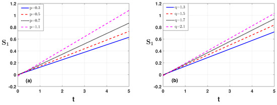
Figure 1. Condition $S_1$ of Example 1 is plotted against the time variable t for (a) varying index $\mathfrak{p}$ and (b) varying index $\mathfrak{q}$.

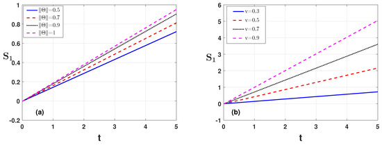
Figure 2. Condition $S_1$ of Example 1 is plotted against the time variable t for (a) varying the parameter $\parallel \Theta \parallel$ and (b) varying the parameter $\zeta$.

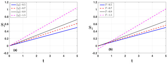
Figure 3. Condition $S_1$ of Example 1 is plotted against the time variable t for (a) varying the parameter $\parallel \chi \parallel$ and (b) varying the parameter T.

Table 1. Evaluation of the condition $S_1$ for different values of $\mathfrak{p}$, $\mathfrak{q}$, and t.

t	$\mathbf{(}\mathfrak{p}\mathbf{,}\mathfrak{q}\mathbf{)}\mathbf{=}\mathbf{(}\mathbf{1}\mathbf{/}\mathbf{5}\mathbf{,}\mathbf{3}\mathbf{/}\mathbf{2}\mathbf{)}$	$(\mathfrak{p},\mathfrak{q})=(2/5,5/3)$	$(\mathfrak{p},\mathfrak{q})=(3/5,7/4)$	$(\mathfrak{p},\mathfrak{q})=(4/5,9/5)$	$(\mathfrak{p},\mathfrak{q})=(1,2)$
0.0	0.193696	0.533696	0.793696	0.993696	1.193696
0.2	0.533696	0.55369	0.733696	0.835696	1.543696
0.4	0.835696	0.855696	0.875696	0.835696	1.435696
0.6	0.635696	0.735696	0.935696	0.933696	1.535696
0.8	0.535696	0.835696	0.935696	0.9835696	1.363596
1.0	0.935696	0.9355696	0.935696	1.935696	1.936962

Next, to check condition $S_2$ of Example 2, we choose the parameters $\parallel \xi \parallel =2/15$, $\parallel \zeta \parallel =4/5$, $\parallel \varphi \parallel =3/20$, and $\parallel \chi \parallel =1/3$. In Figure 4a, we depict the condition $S_2$ against the time variable t for the time indices’ values $\mathfrak{p}$ and $\mathfrak{q}$, respectively. We see that, with the enhancement of both of these indices, the condition $S_2$ obtains larger values and exceeds their limit. Similar results are shown in Figure 5a,b by changing the parameter values $\Theta$ and $\gamma$. The effects of the parameters are shown there. The effects of the parameters $\chi$ and T are shown in Figure 6a,b. The numerical analysis for the effect of the parameters $\mathfrak{p}$ and $\mathfrak{q}$ is also shown in Table 2 for condition $S_2.$ In Examples 3 and 4, we derive the existence results for the BVP in the form of hybrid fractional and hybrid fractional integro-order derivatives, respectively.

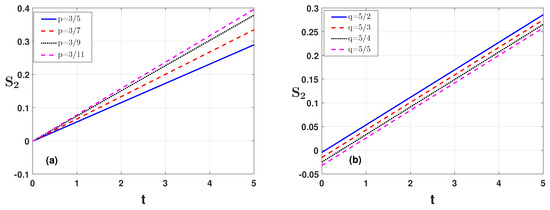
Figure 4. Condition $S_2$ of Example 2 is plotted against the time variable t for (a) varying the parameter $\mathfrak{p}$ and (b) varying the parameter $\mathfrak{q}$.

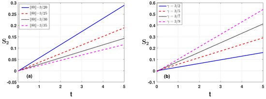
Figure 5. Condition $S_2$ of Example 2 is plotted against the time variable t for (a) varying the parameter $\parallel \Theta \parallel$ and (b) varying the parameter $\gamma$.

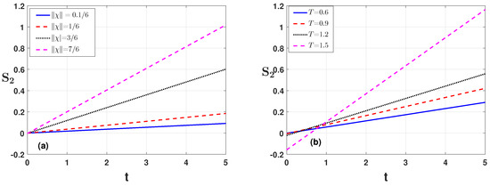
Figure 6. Condition $S_2$ of Example 1 is plotted against the time variable t for (a) varying the parameter $\parallel \chi \parallel$ and (b) varying the parameter T.

Table 2. Evaluation of the condition $S_2$ for different values of $\mathfrak{p}$, $\mathfrak{q}$, and t.

t	$(\mathfrak{p},\mathfrak{q})=(1/2,5/2)$	$(\mathfrak{p},\mathfrak{q})=(2/3,7/3)$	$(\mathfrak{p},\mathfrak{q})=(3/5,9/4)$	$(\mathfrak{p},\mathfrak{q})=(4/5,11/5)$	$(\mathfrak{p},\mathfrak{q})=(1,2)$
0.0	0.093696	0.433696	0.693696	0.893696	1.193696
0.2	0.433696	0.653694	0.933696	0.835666	1.543696
0.4	0.435696	0.755696	0.955696	0.985636	1.673696
0.6	0.735696	0.835696	0.935696	0.973696	1.835696
0.8	0.535396	0.835396	0.935396	0.983366	1.363396
1.0	0.735396	0.833566	0.975636	1.985636	1.736932

8. Conclusions

We established an existence theory for the proposed BVP (2) of the hybrid fractional sequential integro-differential (HFSID) equation in response to Dhage’s [26] and Jamil’s [28] applied generalized Krasnoselikii’s fixed-point theorem on the BVP. We also demonstrated the problem’s Ulam stability, identified as Ulam–Hyers and Ulam–Hyers–Rassias stability. With the help of the Arzelà–Ascoli Theorem 1 and Lemma 2, we proved that the result obtained as (17) of the BVP (2) exists and is unique. Finally, four examples with the numerical plots and discussions were illustrated to verify our results. The effects of the different parameters were shown to verify the results obtained in this manuscript. The numerical illustration of the BVPs investigated that the existence and uniqueness results with Ulam stability comprise one of the challenging tasks to investigate for such problems [32,33,34,35,36,37]. The physical systems in the fields of plasma physics, electrical engineering, and biological models, hybrid fractional sequential integro-differential equations (HFSID) play a key role due to their double-fractional-order derivative. In such physical systems, the time derivative terms need to be integrated with a continuous change. Hence, the HFSID could play a novel key role in overcoming such problems.

As future work, it will be interesting to investigate the hybrid planar waveguide arrays by a variety of fractional coupled sine-Gordon equations with different phase shifts reported in [38] for the integer order. The consideration of such systems is very useful to investigate different physical phenomena for the applications of the parity time symmetry in optics, Bose–Einstein condensates, and nonlinear physical phenomena, where the coupling of nonlinearity fundamentally advances the problem and generates completely novel characteristics.

References

- Kilbas, A.A.; Srivastava, H.M.; Trujillo, J.J. Theory and Applications of Fractional Differential Equations; North-Holland Mathematics Studies; Elsevier: Amsterdam, The Netherlands, 2006; Volume 204. [Google Scholar]
- Lakshmikantham, V.; Leela, S.; Vasundhara Devi, J. Theory of Fractional Dynamic Systems; Cambridge Academic Publishers: Cambridge, UK, 2009. [Google Scholar]
- Yasmin, H.; Iqbal, N.A. Comparative Study of the Fractional Coupled Burgers and Hirota–Satsuma KdV Equations via Analytical Techniques. Symmetry 2022, 14, 1364. [Google Scholar] [CrossRef]
- Shah, N.; Alyousef, H.; El-Tantawy, S.; Shah, R.; Chung, J. Analytical Investigation of Fractional-Order Korteweg-De-Vries-Type Equations under Atangana-Baleanu-Caputo Operator: Modeling Nonlinear Waves in a Plasma and Fluid. Symmetry 2022, 14, 739. [Google Scholar] [CrossRef]
- Irina, A.; Koresheva, E. Estimation of the FST-Layering Time for Shock Ignition ICF Targets. Symmetry 2022, 14, 1322. [Google Scholar]
- Gulaly, S.; Ali, A.; Ahmad, S.; Nonlaopon, K.; Akgül, A. Bright Soliton Behaviours of Fractal Fractional Nonlinear Good Boussinesq Equation with Nonsingular Kernels. Symmetry 2022, 14, 2113. [Google Scholar]
- Pruchnicki, E. Two New Models for Dynamic Linear Elastic Beams and Simplifications for Double Symmetric Cross-Sections. Symmetry 2022, 14, 1093. [Google Scholar] [CrossRef]
- Candan, M. Some Characteristics of Matrix Operators on Generalized Fibonacci Weighted Difference Sequence Space. Symmetry 2022, 14, 1283. [Google Scholar] [CrossRef]
- Ali, A.; Khan, A.U.; Algahtani, O.; Saifullah, S. Semi-analytical and numerical computation of fractal-fractional sine-Gordon equation with non-singular kernels. AIMS Math. 2022, 7, 14975–14990. [Google Scholar] [CrossRef]
- Podlubny, I. Fractional Differential Equations; Academic Press: San Diego, CA, USA, 1999. [Google Scholar]
- Sabatier, J.; Agrawal, O.P.; Machado, J.A.T. (Eds.) Advances in Fractional Calculus: Theoretical Developments and Applications in Physics and Engineering; Springer: Dordrecht, Germany, 2007. [Google Scholar]
- Odibat, Z.M. Computing eigenelements of boundary value problems with fractional derivatives. Appl. Math. Comput. 2009, 215, 3017–3028. [Google Scholar] [CrossRef]
- Stojanović, M. Numerical method for solving diffusion-wave phenomena. J. Comput. Appl. Math. 2011, 235, 3121–3137. [Google Scholar] [CrossRef]
- Zhao, Y.; Sun, S.; Han, Z.; Li, Q. Theory of fractional hybrid differential equations. Comput. Math. Appl. 2011, 62, 1312–1324. [Google Scholar] [CrossRef]
- Sun, S.; Zhao, Y.; Han, Z.; Li, Y. The existence of solutions for boundary value problem of fractional hybrid differential equations. Commun. Nonlinear Sci. Numer. Simul. 2012, 17, 4961–4967. [Google Scholar] [CrossRef]
- Ahmad, B.; Ntouyas, S.K. An existence theorem for fractional hybrid differential inclusions of Hadamard type with Dirichlet boundary conditions. Abstr. Appl. Anal. 2014, 2014, 705809. [Google Scholar] [CrossRef]
- Dhage, B.C.; Ntouyas, S.K. Existence results for boundary value problems for fractional hybrid differential inclusions. Topol. Methods Nonlinear Anal. 2014, 44, 229–238. [Google Scholar] [CrossRef]
- Zhao, Y.; Wang, Y. Existence of solutions to boundary value problem of a class of nonlinear fractional differential equations. Adv. Differ. Equ. 2014, 174, 1–10. [Google Scholar] [CrossRef]
- Miller, K.S.; Ross, B. An Introduction to Fractional Calculus and Fractional Differential Equations; Wiley: New York, NY, USA, 1993. [Google Scholar]
- Wei, Z.; Dong, W. Periodic boundary value problems for Riemann–Liouville sequential fractional differential equations. Electron. J. Qual. Theory Differ. Equ. 2011, 87, 1–13. [Google Scholar] [CrossRef]
- Wei, Z.; Li, Q.; Che, J. Initial value problems for fractional differential equations involving Riemann–Liouville sequential fractional derivative. J. Math. Anal. Appl. 2010, 367, 260–272. [Google Scholar] [CrossRef]
- Hyers, D.H. On the stability of the linear functional equation. Proc. Natl. Acad. Sci. USA 1941, 27, 222–224. [Google Scholar] [CrossRef]
- Jung, S.M. On the Hyers–Ulam stability of the functional equations that have the quadratic property. J. Math. Anal. Appl. 1998, 222, 126–137. [Google Scholar] [CrossRef]
- Jung, S.M. Hyers–Ulam stability of linear differential equations of first order II. Appl. Math. Lett. 2006, 19, 854–858. [Google Scholar] [CrossRef]
- Obloza, M. Hyers stability of the linear differential equation. Rocz. Nauk Dydakt. Prace Mat. 1993, 13, 259–270. [Google Scholar]
- Dhage, B.C.; Lakshmikantham, V. Basic results on hybrid differential equations. Nonlinear Anal. 2010, 4, 414–424. [Google Scholar] [CrossRef]
- Shete, A.Y.; Bapurao, C.D.; Namdev, S.J. Differential inequalities for a finite system of hybrid Caputo fractional differential equations. Adv. Inequal. Appl. 2014, 2014, 35. [Google Scholar]
- Jamil, M.; Khan, R.A.; Shah, K. Existence theory to a class of boundary value problems of hybrid fractional sequential integro-differential equations. Bound. Value Probl. 2019, 1, 1–12. [Google Scholar] [CrossRef]
- Khan, R.A.; Shah, K. Existence and uniqueness of solutions to fractional order multi-point boundary value problems. Commun. Appl. Anal. 2015, 19, 515–526. [Google Scholar]
- Rus, I.A. Ulam stabilities of ordinary differential equations in a Banach space. Carpathian J. Math. 2010, 26, 103–107. [Google Scholar]
- Sabirova, R. Fractional differential equations: Change of variables and nonlocal symmetries. J. Math. Probl. Equ. Stat. 2021, 2, 44–59. [Google Scholar]
- Gul, Z.; Ali, A. Localized modes in a variety of driven long Josephson junctions with phase shifts. Nonlinear Dyn. 2018, 94, 229–247. [Google Scholar] [CrossRef]
- Zhang, L.; ur Rahman, M.; Arfan, M.; Ali, A. Investigation of mathematical model of transmission co-infection TB in HIV community with a non-singular kernel. Results Phys. 2021, 28, 104559. [Google Scholar] [CrossRef]
- Din, Z.U.; Ali, A.; De la Sen, M.; Zaman, G. Entropy generation from convective–radiative moving exponential porous fins with variable thermal conductivity and internal heat generations. Sci. Rep. 2022, 12, 1791. [Google Scholar]
- Din, Z.U.; Ali, A.; Ullah, S.; Zaman, G.; Shah, K. and Mlaiki, N. Investigation of heat transfer from convective and radiative stretching/shrinking rectangular fins. Math. Probl. Eng. 2022, 2022. [Google Scholar] [CrossRef]
- Khan, K.; Algahtani, O.; Irfan, M.; Ali, A. Electron-acoustic solitary potential in nonextensive streaming plasma. Sci. Rep. 2022, 12, 15175. [Google Scholar] [CrossRef] [PubMed]
- Khan, K.; Ali, A.; Irfan, M.; Algahtani, O. Time-fractional electron-acoustic shocks in magnetoplasma with superthermal electrons. Alex. Eng. J. 2022. [Google Scholar] [CrossRef]
- Khan, W.A.; Ali, A.; Gul, Z.; Ahmad, A.; Ullah, A. Localized modes in PT-symmetric sine-Gordon couplers with phase shift. Chaos Solitons Fractals 2020, 139, 110290. [Google Scholar] [CrossRef]
Publisher’s Note: MDPI stays neutral with regard to jurisdictional claims in published maps and institutional affiliations. |
© 2022 by the author. Licensee MDPI, Basel, Switzerland. This article is an open access article distributed under the terms and conditions of the Creative Commons Attribution (CC BY) license (https://creativecommons.org/licenses/by/4.0/).