The σ₋ Cohomology Analysis for Symmetric Higher-Spin Fields

Abstract

In this paper, we present a complete proof of the so-called First On-Shell Theorem that determines dynamical content of the unfolded equations for free symmetric massless fields of arbitrary integer spin in any dimension and arbitrary integer or half-integer spin in four dimensions. This is achieved by calculation of the respective ${\sigma }_{-}$ cohomology both in the tensor language in Minkowski space of any dimension and in terms of spinors in $Ad{S}_4$. In the d-dimensional case $H^p\left({\sigma }_{-}\right)$ is computed for any p and interpretation of $H^p\left({\sigma }_{-}\right)$ is given both for the original Fronsdal system and for the associated systems of higher form fields.

1. Introduction

Higher-spin (HS) gauge theory is based on works of Fronsdal [1] and Fang and Fronsdal [2], where the action and equations of motion for massless gauge fields of any spin were originally obtained in flat four-dimensional Minkowski space. Even earlier, important restrictions on low-energy HS vertices were obtained by Weinberg in [3,4] and so-called no-go theorems restricting S-matrix possessing too high symmetries in flat space-time were proven in [5,6]. (For a review see [7].) The no-go theorems implied the existence of the $s=2$ barrier suggesting that the construction of an interacting local HS theory in Minkowski space-time is impossible. The proof of these theorems essentially uses the specific form of the algebra of isometries of Minkowski space. The $s=2$ barrier in flat space can be overcome in the space-time with non-zero sectional curvature, for example, in the anti-de Sitter space [8]. In these spaces it becomes possible to formulate a consistent nonlinear theory of fields of all spins [9,10].

The construction of a nonlinear HS theory is essentially based on the so-called unfolded approach [11,12], which is a far-going generalization of the Cartan formulation of gravity ($s=2$) in terms of differential forms to fields of any spin $s>2$. Via introducing appropriate auxiliary variables, the unfolding procedure allows one to replace the system of partial differential equations of any order on a smooth manifold by a larger system of first-order equations on vector-valued differential forms. One of the essential features of this approach, which is very useful for analysing symmetries of a given system, is that the variables in the equations are valued in one or another representation of the underlying symmetry algebra.

The dynamical content of the HS theory can be reconstructed from its unfolded formulation using the ${\sigma }_{-}$ cohomology technique [13]. As is recalled below, the dynamical data of the theory are in one-to-one correspondence with the cohomology of certain linear nilpotent operator ${\sigma }_{-}$ that can be read of the unfolded equations in question. The statement that unfolded equations of free HS fields are equivalent to the Fronsdal equations was made in the original papers in the spinor [14] and tensor [15] formalisms. In the tensor formulation of HS theory the idea of the proof was illustrated in [16], where however the analysis of the trace part of the Fronsdal equations was not completed, while general arguments for mixed-symmetry HS fields were given in [17]. In [18] the unfolded equations for massless fields were derived from the Fronsdal theory by the BRST methods. To the best of our knowledge, no detailed analysis of the problem in the spinor formalism was available in the literature.

In this paper we present a complete proof of the so called First On-Shell Theorem by computation of the cohomology rings of ${\sigma }_{-}$ for the physically important cases of the integer-spin symmetric fields both in flat space-time of any dimension and $Ad{S}_d$ as well as for the fields of any integer and half-integer spin in ${AdS}_4$. The computation technique analogous to the Hodge theory for differential forms is performed in terms of so-called ${\sigma }_{-}$ cohomology and provides a complete analysis of the dynamical content of the free unfolded equations for symmetric massless fields of any spin. Giving a direct proof of the equivalence between the Fronsdal formulation of the HS gauge theory and its unfolded formulation this paper fills in some gaps in the literature also illustrating a general approach applicable to a broad class of unfolded systems. In addition, in the tensor case we compute higher ${\sigma }_{-}$ cohomology groups and interpret them in terms of higher Bianchi identities and more general dynamical systems. In particular, we discuss the matching between the Bianchi identities in terms of one-form gauge fields and zero-form field strengths.

The rest of the paper is organized as follows. In Section 2 we briefly recall different approaches to the description of HS massless fields. Main idea of the ${\sigma }_{-}$ cohomology approach is explained in Section 3. Cohomology calculation method used in this paper is discussed in Section 4. Section 5 contains derivation of $H^p\left({\sigma }_{-}\right)$ in Minkowski space of any dimension. In particular, the cases of $\mathrm{GL}\left(d\right)$ and $\mathrm{O}\left(d\right)$ representations are analysed here. In Section 6 calculation of the low-order cohomology groups in $Ad{S}_4$ is performed. Obtained results are discussed in Section 7. Index conventions and normalisations of the tensor Young diagrams are presented in the Appendix A.

2. Fronsdal Theory

2.1. Metric Formulation

According to Fronsdal [1], a spin-s massless symmetric field can be described in terms of two symmetric traceless tensors (for index conventions see Appendix A)

$$\begin{array}{c}\hfill {\varphi }^{a\left(s\right)}\equiv {\varphi }^{a_1..a_s},{\varphi }^{a(s-2)}\equiv {\varphi }^{a_1..a_{s-2}},{\eta }_{b_1{b}_2}{\varphi }^{b_1{b}_2{a}_3..a_s}\equiv {{\varphi }^{a(s-2)b}}_b=0,{{\varphi }^{a(s-4)b}}_b=0.\end{array}$$

(1)

These two fields can be combined into a single rank-s totally symmetric tensor

$${\phi }^{a\left(s\right)}={\varphi }^{a\left(s\right)}+{\eta }^{aa}{\varphi }^{a(s-2)}$$

(2)

obeying the double-tracelessness condition

$${{\phi }^{a(s-4)bc}}_{bc}=0.$$

(3)

The field equations in Fronsdal theory have the form

$$R^{a\left(s\right)}\left(\phi \right)=\square {\phi }^{a\left(s\right)}-s{\partial }^a{\partial }_k{\phi }^{ka(s-1)}+\frac{s(s-1)}{2}{\partial }^a{\partial }^a{{\phi }^{a(s-2)k}}_k=0,$$

(4)

where ${\partial }_a=\frac{\partial }{\partial x^a}$.

The tensor $R^{a\left(s\right)}\left(\phi \right)$ is invariant under the gauge transformations with a rank-$(s-1)$ traceless gauge parameter $\epsilon \left(x\right)$

$$\delta {\phi }^{a\left(s\right)}={\partial }^a{\epsilon }^{a(s-1)},{{\epsilon }^{a(s-3)k}}_k=0.$$

(5)

Fronsdal Equation (4) is a generalization of the well-known equations of fields with spins $s=0,1,2$. For the case of $s=1$ the last term in the Fronsdal tensor disappears and Equation (4) reproduces Maxwell equations for the field $A^a$. Without the last two terms at $s=0$ it gives Klein-Gordon equation for a massless scalar field. The case of $s=2$ reproduces the equations of linearized gravity [19]. Gauge transformation (5) gives the known gauge transformations of low-spin fields and its absence for a scalar field.

2.2. Frame-Like Formulation

2.2.1. Tensor Formalism

The unified description of massless fields of arbitrary spin can be given in the so-called frame-like formalism that generalizes Cartan formulation of gravity, operating in terms of differential forms [14,15,20]. Frame-like formulation of the HS gauge theory in any dimension is given in terms of the one-form fields ${\omega }^{a(s-1),b\left(t\right)}=d{x}^{\nu }{\omega }_{\nu }^{a(s-1),b\left(t\right)}$ valued in two-row Young diagrams corresponding to irreducible $\mathfrak{o}(d-1,1)$ (i.e., traceless) modules [15], obeying conditions

$$\begin{array}{cc}\hfill & {\omega }^{a(s-1),ab(t-1)}=0,\hfill \end{array}$$

(6)

$$\begin{array}{cc}\hfill & {{{\omega }^{a(s-3)k}}_k}^{,b\left(t\right)}=0.\hfill \end{array}$$

(7)

(For index conventions see Appendix A).

By introducing auxiliary fields it is possible to put a system of partial differential equations into the first-order unfolded form [11,12]. Generally, unfolded equations read as

$$d{W}^A=\sum _{n=1}^{\infty }{G}_{B_1,..,B_n}^A{W}^{B_1}\wedge ...\wedge W^{B_n},d:=d{x}^{\nu }{\partial }_{\nu }.$$

(8)

Here $W^A$ is a set of differential forms over some manifold. (Indices are treated formally and can take an infinite number of values.) The coefficients $G_{B_1,..,B_n}^A$ satisfy the (anti)symmetry condition

$$G_{B_1,..,B_i,..,B_j,..,B_n}^A={(-1)}^{|B_i\left|\right|B_j|}{G}_{B_1,..,B_j,..,B_i,..,B_n}^A,$$

(9)

where $|B_i|$ denotes the form-degree of $W^{B_i}$. Also $G_{B_1,..,B_n}^A$ are restricted by the integrability conditions expressing that $d^2=0$.

In the tensor language the unfolded HS equations in Minkowski space proposed in [15] read as

$$D_L{\omega }^{a(s-1),b\left(t\right)}+h_m\wedge {\omega }^{a(s-1),b\left(t\right)m}=0,t\in \{0,..,s-2\},$$

(10)

$$D_L{\omega }^{a(s-1),b(s-1)}=h_n\wedge h_m\wedge C^{a(s-1)n,b(s-1)m},$$

(11)

where $h_n$ is a soldering form (vielbein, frame field, tetrad) and $D_L=d+\varpi$ is the background Lorentz covariant derivative that satisfies relations

$$D_L{h}^a=0,D_L^2=0.$$

(12)

In the Cartesian coordinate system with $\varpi =0$ the equations simplify to

$$d{\omega }^{a(s-1),b\left(t\right)}+h_m\wedge {\omega }^{a(s-1),b\left(t\right)m}=0,t\in \{0,..,s-2\},$$

(13)

$$d{\omega }^{a(s-1),b(s-1)}=h_n\wedge h_m\wedge C^{a(s-1)n,b(s-1)m},$$

(14)

where C satisfies the Lorentz irreducibility conditions

$$C^{a\left(n\right),ab(m-1)}=0,{{C^{a(n-2)k}}_k}^{,b\left(m\right)}=0.$$

(15)

The traceless tensor C on the r.h.s. of (14) is a generalized Weyl tensor. There are also unfolded equations on C and on additional auxiliary fields [10] (for reviews see [16,21]). This system constitutes an infinite chain of zero-form equations. Zero-form sector, that contains equations on spin-zero and spin-one fields, will not be considered in this paper.

Equations (13) are invariant under the gauge transformations

$$\delta {\omega }^{a(s-1),b\left(t\right)}=d{\epsilon }^{a(s-1),b\left(t\right)}+h_m{\epsilon }^{a(s-1),b\left(t\right)m},t\in \{0,..,s-2\}$$

(16)

and Equation (14) is invariant under

$$\begin{array}{cc}\hfill & \delta {\omega }^{a(s-1),b(s-1)}=d{\epsilon }^{a(s-1),b(s-1)},\hfill \end{array}$$

(17)

$$\begin{array}{cc}\hfill & \delta C^{a\left(s\right),b\left(s\right)}=0,\hfill \end{array}$$

(18)

where $\epsilon$ are zero-forms valued in the appropriate two-row irreducible $\mathfrak{o}(d-1,1)$-modules obeying conditions analogous to (15).

The Fronsdal field is embedded into the frame-like one-form $e^{a(s-1)}\equiv {\omega }^{a(s-1)}$ in the following manner. Converting the form index into the fiber one using vielbein h,

$$e^{a(s-1)|b}=e_{\mu }^{a(s-1)}{h}^{\mu b},$$

(19)

the resulting tensor (19) can be decomposed into irreducible $\mathfrak{o}(d-1,1)$-modules. In terms of traceless Young diagrams this decomposition is

(20)

The first two components give the Fronsdal field, while the third one is an excess of the components of the frame-like field in comparison with the Fronsdal field. At the tensor level, this decomposition is represented as:

$$e^{a(s-1)|b}={\psi }_1^{a(s-1)b}+{\beta }_1{\eta }^{aa}{\psi }_2^{a(s-3)b}+{\beta }_2{\eta }^{ab}{\psi }_2^{a(s-2)}+{\psi }_3^{a(s-1),b},$$

(21)

where ${\psi }_i$ are traceless and correspond to the i-th diagram. The relative coefficient $\frac{{\beta }_2}{{\beta }_1}$ is fixed by the tracelessness condition with respect to indices a.

This decomposition shows that the Fronsdal field identifies with the symmetric part of the frame-like field, since the contribution of the third diagram disappears upon symmetrization. The resulting field

$${\phi }^{a\left(s\right)}:=e^{a(s-1)|a}$$

(22)

is symmetric and double-traceless. The extra term ${\psi }_3^{a(s-1),b}$ is pure gauge. Its contribution can be canceled by the gauge transformation $\delta e^{a(s-1)|b}={\epsilon }^{a(s-1)|b}$ with suitable gauge parameter. For detailed discussion of Fronsdal field embedding see [16,20,21].

It is not difficult to check [15,20] (for reviews see [16,21]) that the Fronsdal equations and gauge transformations follow from the unfolded system (13), (14). A more complicated question is whether the Fronsdal fields and equations are the only ones that result from (13), (14). The answer can be obtained via the ${\sigma }_{-}$ cohomology technique [13].

2.2.2. Spinor Language in $Ad{S}_4$

The physically important case of the unfolded system for HS connection (13), (14) is that of $Ad{S}_4$ space-time in which case the language of two-component spinors is most appropriate. In this language instead of using Lorentz indices $a,b,...=0,1,2,3$, one uses two pairs of dotted and undotted spinor indices $\alpha ,\beta , \dots$ and $\dot{\alpha },\dot{\beta }, \dots$ taking values $\{1,2\}$. The two languages are related via Pauli matrices. The $Ad{S}_4$ background geometry is described in terms of the Lorentz connection $\varpi$ and frame field h, that satisfy equations

$$\begin{array}{c}d{h}^{\alpha \dot{\beta }}+{{\varpi }^{\alpha }}_{\gamma }\wedge h^{\gamma \dot{\beta }}+{{\overline{\varpi }}^{\dot{\beta }}}_{\dot{\gamma }}\wedge h^{\alpha \dot{\gamma }}=0,\hfill \\ d{\varpi }^{\alpha \beta }+{{\varpi }^{\alpha }}_{\gamma }\wedge {\varpi }^{\gamma \beta }=-{\lambda }^2{h^{\alpha }}_{\dot{\gamma }}\wedge h^{\beta \dot{\gamma }},\hfill \\ d{\overline{\varpi }}^{\dot{\alpha }\dot{\beta }}+{{\overline{\varpi }}^{\dot{\alpha }}}_{\dot{\gamma }}\wedge {\overline{\varpi }}^{\dot{\gamma }\dot{\beta }}=-{\lambda }^2{h_{\gamma }}^{\dot{\alpha }}\wedge h^{\gamma \dot{\beta }},\hfill \end{array}$$

(23)

where ${\lambda }^2$ is proportional to the curvature of $Ad{S}_4$ and we adopt the following rules

$$A_{\alpha }=A^{\beta }{ϵ}_{\beta \alpha },A^{\alpha }={ϵ}^{\alpha \beta }{A}_{\beta },{ϵ}_{\alpha \beta }{ϵ}^{\gamma \beta }={{ϵ}_{\alpha }}^{\gamma }={\delta }_{\alpha }^{\gamma }=-{{ϵ}^{\gamma }}_{\alpha },$$

(24)

where

$${ϵ}_{\alpha \beta }=-{ϵ}_{\beta \alpha },{ϵ}_{12}=1.$$

(25)

The spinor version of the unfolded system for one-form $\omega$ reads as follows. First, the HS curvatures in the spinor language are [14]

$$R^{\alpha \left(n\right),\dot{\alpha }\left(m\right)}=D_L{\omega }^{\alpha \left(n\right),\dot{\alpha }\left(m\right)}+{\lambda }^2(n{h}_{\dot{\gamma }}^{\alpha }\wedge {\omega }^{\alpha (n-1),\dot{\gamma }\dot{\alpha }\left(m\right)}+m{h}_{\gamma }^{\dot{\alpha }}\wedge {\omega }^{\gamma \alpha \left(n\right),\dot{\alpha }(m-1)})$$

(26)

and $D_L=d+\varpi +\overline{\varpi }$ is a Lorentz-covariant derivative with Cartan’s spin-connection $(\varpi \oplus \overline{\varpi })$

$$D_L{\omega }^{\alpha \left(n\right),\dot{\alpha }\left(m\right)}=d{\omega }^{\alpha \left(n\right),\dot{\alpha }\left(m\right)}+n{\varpi }_{\alpha }^{\beta }\wedge {\omega }_{\beta \alpha (n-1),\dot{\alpha }\left(m\right)}+m{\overline{\varpi }}_{\dot{\alpha }}^{\dot{\beta }}\wedge {\omega }_{\alpha \left(n\right),\dot{\beta }\dot{\alpha }(m-1)}.$$

The $Ad{S}_4$ deformation of the unfolded Equations (13) and (14) then takes the form [12]

$$R^{\alpha \left(n\right),\dot{\alpha }\left(m\right)}={\delta }_{0,n}{h}_{\beta \dot{\alpha }}\wedge h_{\dot{\alpha }}^{\beta }{\overline{C}}^{\dot{\alpha }(m+2)}+{\delta }_{0,m}{h}_{\alpha \dot{\beta }}\wedge h_{\alpha }^{\dot{\beta }}{C}^{\alpha (n+2)}.$$

(27)

The main advantage of the two-component spinor notation is that it makes the representation theory of the Lorentz group very simple. Namely, every Lorentz irreducible multispinor representing a traceless tensor is totally symmetric in its spinor indices. Since the only Lorentz invariant objects are antisymmetric bispinors ${ϵ}_{\alpha \beta }$ and ${\overline{ϵ}}_{\dot{\alpha }\dot{\beta }}$ irreducible multispinors $X^{\alpha \left(n\right),\dot{\alpha }\left(m\right)}$ are necessarily symmetric with respect to the indices in the groups $\alpha \left(n\right)$ and $\dot{\alpha }\left(m\right)$ separately. Thus, working with the two-component spinor notation one can happily forget about painful calculations with the traces of Lorentz-tensors.

3. The Idea of ${\mathbf{\sigma }}_{-}$ Cohomology Analysis: Example of Integer Spin Massless Fields

The l.h.s.’s of unfolded HS equations and gauge transformations in d-dimensional Minkowski space are [15,16]

$$\begin{array}{cc}\hfill & R^{a(s-1),b\left(k\right)}=D_L{\omega }^{a(s-1),b\left(k\right)}+{\sigma }_{-}{\left(\omega \right)}^{a(s-1),b\left(k\right)},\hfill \end{array}$$

(28)

$$\begin{array}{cc}\hfill & \delta {\omega }^{a(s-1),b\left(k\right)}=D_L{\epsilon }^{a(s-1),b\left(k\right)}+{\sigma }_{-}{\left(\epsilon \right)}^{a(s-1),b\left(k\right)},\hfill \end{array}$$

(29)

where

$${\left({\sigma }_{-}\omega \right)}^{a(s-1),b\left(k\right)}:=h_c\wedge {\omega }^{a(s-1),b\left(k\right)c},{\left({\sigma }_{-}\epsilon \right)}^{a(s-1),b\left(k\right)}:=h_c\wedge {\epsilon }^{a(s-1),b\left(k\right)c}.$$

(30)

$R^{a(s-1),b\left(k\right)}$ is referred to as (linearized) HS curvature. For simplicity we study the Minkowski case. Since ${\sigma }_{-}$ in $Ad{S}_d$ is defined analogously, our analysis applies to that case as well.

Due to their definition, HS curvatures obey the Bianchi identities

$$D_L{R}^{a(s-1),b\left(k\right)}+{\sigma }_{-}{\left(R\right)}^{a(s-1),b\left(k\right)}=0.$$

(31)

The appearance of ${\sigma }_{-}$ allows one to clarify the role of the fields ${\omega }^{a(s-1),b\left(k\right)}$ and gauge parameters ${\epsilon }^{a(s-1),b\left(k\right)}$. Working with the zero-forms ${\epsilon }^{a(s-1),b\left(k\right)}$ and one-forms ${\omega }^{a(s-1),b\left(k\right)}$ valued in two-row Young diagrams, we consider the space $V^p$ of p-forms valued in two-row Young diagrams with any p. Defining ${\sigma }_{-}$ to annihilate the forms with an empty second row, we find that ${\sigma }_{-}{V}^p\subset V^{p+1}$ and ${\sigma }_{-}{\sigma }_{-}=0$. As originally proposed in [13], the ${\sigma }_{-}$ cohomology $H\left({\sigma }_{-}\right)=ker\left({\sigma }_{-}\right)/\mathrm{im}\left({\sigma }_{-}\right)$ classifies fields, their equations and gauge symmetries.

Indeed, those components of the fields ${\omega }^{a(s-1),b\left(t\right)}$, that are not annihilated by ${\sigma }_{-}$, can be expressed via derivatives of the fields with lower t by setting suitable components of the HS curvatures to zero. Such fields are called auxiliary. Conversely, those components of the fields ${\omega }^{a(s-1),b\left(t\right)}$, that cannot be expressed in terms of derivatives of lower fields via zero-curvature conditions, are in $ker\left({\sigma }_{-}\right)$. By Stueckelberg fields we mean ${\sigma }_{-}$-exact fields (i.e., fields of the form ${\sigma }_{-}\chi$) as they can be eliminated by an appropriate ${\sigma }_{-}$-exact term in the gauge transformation (29). Fields that are not expressed via derivatives of other fields and are not Stueckelberg are called dynamical. These describe the physical degrees of freedom of the theory. Thus, the dynamical HS fields are associated with $H^1\left({\sigma }_{-}\right)$.

The classification for the gauge parameters is analogous. The parameters, that are not annihilated by ${\sigma }_{-}$, describe algebraic Stueckelberg shifts. The leftover symmetries are described by the parameters in $ker\left({\sigma }_{-}\right)$. ${\sigma }_{-}$-exact parameters correspond to the so called gauge for gauge transformations. Parameters, which are ${\sigma }_{-}$-closed and not ${\sigma }_{-}$-exact, are referred to as genuine differential gauge parameters. Note that since in the HS example in question the gauge parameters are zero-forms there is no room for gauge for gauge symmetries in that case.

Let V be a graded vector space, $\mathcal{C}$ be an element of ${\mathsf{\Lambda }}^p\left({\mathcal{M}}^d\right)\otimes V$ over some smooth d-dimensional manifold ${\mathcal{M}}^d$. We demand the grading of V to be bounded from below, that is V is $\mathbb{N}$-graded. Let ${\sigma }_{\pm }$ be operators that act ”vertically”, i.e., do not affect the space-time coordinates, and shift grading by $\pm 1$, $D_L$ be the Grassmann-odd operator that does not affect the grading and is allowed to act non-trivially on the space-time coordinates. Consider the covariant constancy condition of a general form along with the zero-curvature condition

$$\mathcal{D}\mathcal{C}=(D_L+{\sigma }_{-}+{\sigma }_{+})\mathcal{C}=0,{\mathcal{D}}^2=0.$$

(32)

Notice that Equation (32) remains invariant under the gauge transformations

$$\delta \mathcal{C}=\mathcal{D}\epsilon ,$$

(33)

where $\epsilon \in {\mathsf{\Lambda }}^{p-1}\left({\mathcal{M}}^d\right)\otimes V$.

One can prove the following proposition [13] (see also [16,22,23,24]):

Theorem 1.

The following is true:

(1) 

Differential gauge symmetry parameters ε span $H^{p-1}\left({\sigma }_{-}\right)$

(2) 

Nontrivial dynamical fields $\mathcal{C}$ span $H^p\left({\sigma }_{-}\right)$

(3) 

Physically distinguishable differential field equations on the nontrivial dynamical fields, contained in $\mathcal{D}\mathcal{C}=0$, span $H^{p+1}\left({\sigma }_{-}\right)$

Thus, taking into account that HS gauge fields are described by the one-forms $\omega$, to prove that the Fronsdal metric formulation is equivalent to the unfolded one, we have to calculate $H^0\left({\sigma }_{-}\right),H^1\left({\sigma }_{-}\right)$ and $H^2\left({\sigma }_{-}\right)$. More generally, higher cohomology $H^k\left({\sigma }_{-}\right)$ with $k>p+1$ describes Bianchi identities for dynamical equations at $k=p+2$ and Bianchi for Bianchi identites at $k>p+2$ [24]. Similarly, the lower cohomology $H^k\left({\sigma }_{-}\right)$ with $k<p-1$ describes gauge for gauge differential symmetries.

4. A Method for Calculating Cohomology

Calculation of ${\sigma }_{-}$ cohomology is of utter importance for the analysis of unfolded systems of the general form (32). The straightforward calculation of the cohomology can be quite involved. In this paper we find cohomology using a standard homotopy approach recalled below, that is a generalization of the Hodge theory for de Rham cohomology extendable to a more general class of (co)chain complexes. Main details of the construction used in this paper follow those of [24], where the ${\sigma }_{-}$ cohomology analysis was applied to the conformal HS theories of the bosonic fields of any symmetry type. Unfortunately, some of the methods of [24], based on the fact that ${\sigma }_{-}$ in conformal theories has the clear meaning in terms of the conformal algebra, are not directly applicable to the non-conformal HS theories discussed in this paper, which makes the analysis of the latter a bit more involved.

Let V be a graded vector space and d be a linear operator of degree +1 on V (that is, it raises the grading of a homogeneous element by 1) such that $d^2=0$. Then $H\left(d\right)=ker\left(d\right)/\mathrm{im}\left(d\right)$. Let ∂ be another operator of degree $-1$ on V (i.e., it lowers the grading by 1) such that ${\partial }^2=0$. The operators d and ∂ can be used to compose the degree 0 operator $\mathsf{\Delta }$

$$\mathsf{\Delta }:=\{d,\partial \}=d\partial +\partial d.$$

(34)

It is easy to see that $\mathsf{\Delta }$ satisfies

$$[d,\mathsf{\Delta }]=[\partial ,\mathsf{\Delta }]=0.$$

(35)

Lemma 1.

If Δ is diagonalizable on the (graded) vector space V, then $H\left(d\right)\hookrightarrow ker\left(\mathsf{\Delta }\right)$.

Proof. 

First of all we should show that $ker\left(d\right)$ is an invariant subspace of $\mathsf{\Delta }$. Suppose $f\in ker\left(d\right)$. Then

$$\mathsf{\Delta }f=(d\partial +\partial d)f=d\partial f\Rightarrow \mathsf{\Delta }f\in ker\left(d\right),\forall f\in ker\left(d\right).$$

(36)

Therefore, $ker\left(d\right)$ is an invariant subspace of $\mathsf{\Delta }$, because linearity is obvious.

Since the operator $\mathsf{\Delta }$ is diagonalizable by assumption, we can consider eigenvectors of $\mathsf{\Delta }$. Let g be d-closed and $\mathsf{\Delta }g=\lambda g,\lambda \ne 0$. Then

$$g=\frac{1}{\lambda }\mathsf{\Delta }g=\frac{1}{\lambda }d\partial g.$$

(37)

Hence, g is also d-exact for $\lambda \ne 0$, representing a trivial element of $H\left(d\right)$. Thus, every d-closed form annihilated by $\mathsf{\Delta }$ is not d-exact. In other words, every d-closed form f can be written as $f=h+d\alpha$ with some $h\in ker\left(\mathsf{\Delta }\right)$. □

If V is a Hilbert space with inner product $⟨,⟩$, there exists such ∂ that the converse inclusion $H\left(d\right)\hookleftarrow ker\left(\mathsf{\Delta }\right)$ takes place as well, which means that $H\left(d\right)=ker\left(\mathsf{\Delta }\right)$.

Lemma 2.

Let $(V,⟨,⟩)$ be a Hilbert space, let $d^{*}$ be the operator conjugated to d in the usual sense $⟨\alpha ,d\beta ⟩=⟨d^{*}\alpha ,\beta ⟩$ and $\mathsf{\Delta }=\{d,d^{*}\}$. Then $ker\left(\mathsf{\Delta }\right)\hookrightarrow H\left(d\right)$.

Proof. 

Take any $f\in ker\left(\mathsf{\Delta }\right)$. Then

$$0=⟨f,\mathsf{\Delta }f⟩=⟨df,df⟩+⟨d^{*}f,d^{*}f⟩\iff df=0\mathrm{and}{d}^{*}f=0.$$

(38)

Hence, $f\in ker\left(d\right)$. To show that $f\notin \mathrm{im}\left(d\right)$ suppose the opposite. Let $f=dg$. Then due to (38)

$$d^{*}dg=0\Rightarrow 0=⟨g,d^{*}dg⟩=⟨dg,dg⟩\Rightarrow dg=0.$$

(39)

Thus, $ker\left(\mathsf{\Delta }\right)\hookrightarrow H\left(d\right)$ □

From Lemmas 1 and 2, it follows that, if all the requirements are met,

$$H\left(d\right)=ker\left(\mathsf{\Delta }\right).$$

(40)

Thus, in a Hilbert space with a diagonalizable Laplace operator $\mathsf{\Delta }:=\{d,d^{*}\}$, finding the cohomology is equivalent to finding $ker\left(\mathsf{\Delta }\right)$. Further calculations of ${\sigma }_{-}$ cohomology will rely on this fact.

The following important comment [24] is now in order. In the case of interest, for every unfolded subsystem associated with a fixed spin

$$V={\oplus }_n{V}_n$$

with finite-dimensional grade-n subspaces $V_n$. In that case $\mathsf{\Delta }$ leaves invariant every $V_n$ and, being self-adjoint in the finite-dimensional Hilbert space, is diagonalizable.

It is worth noting the similarity of the above analysis with the Hodge theory mentioned at the beginning of this section. Indeed, consider the (finite-dimensional) vector space V endowed with some nilpotent operators d and ∂, $d^2={\partial }^2=0$. The condition of disjointness is also imposed (see [25] for details), that is, $\mathrm{im}\left(d\right)\cap ker(\partial )=\mathrm{im}(\partial )\cap ker\left(d\right)=\left\{0\right\}$. In other words, it is demanded that

$$\begin{array}{c}\hfill d\partial x=0\mathrm{implies}\partial x=0,\end{array}$$

(41a)

$$\begin{array}{c}\hfill \partial dx=0\mathrm{implies}dx=0.\end{array}$$

(41b)

Define the Laplacian $\mathsf{\Delta }$ by (34). Under these assumptions it can be shown that

• $ker\left(\mathsf{\Delta }\right)=ker\left(d\right)\cap ker(\partial )$. The harmonic cocycles annihilated by $\mathsf{\Delta }$ are those and only those, that are d-closed and ∂-closed simultaneously;
• $V=\mathrm{im}\left(d\right)\oplus \mathrm{im}(\partial )\oplus ker\left(\mathsf{\Delta }\right)$. In other words, for any vector $x\in V$ there exists a unique Hodge decomposition $x=d\alpha +\partial \beta +h$, where $\alpha$ and $\beta$ are some vectors in V, and h is harmonic $\mathsf{\Delta }h=0$.

Since by (41a) $\partial \beta \ne 0$ implies $d\partial \beta \ne 0$, the kernel of d consists of vectors of the type $d\alpha +h$, where h is harmonic,

$$ker\left(d\right)= \left\{x\in V|x=d\alpha +h,\mathsf{\Delta }h=0\right\}.$$

(42)

This implies that the harmonic cocycles and cohomology classes of d are isomorphic as vector spaces, that is (40) is true.

In the subsequent sections the operators ${\sigma }_{-}$ and ${\sigma }_{+}:={\left({\sigma }_{-}\right)}^{*}$ will play the roles of d and ∂. Moreover, in the following calculations one can spot which Young diagram or multispinor belongs to $\mathrm{im}\left({\sigma }_{-}\right),\mathrm{im}\left({\sigma }_{+}\right)$ or $ker\left(\mathsf{\Delta }\right)$ due to the equivariance of the constructed Laplace operators $\mathsf{\Delta }$ with respect to the action of $\mathrm{GL}\left(d\right)$ or $\mathrm{O}\left(d\right)$ or $\mathrm{SL}(2;\mathbb{C})$, depending on the problem in question.

5. ${\mathbf{\sigma }}_{-}$ Cohomology in Minkowski Space of Any Dimension

5.1. Generating Functions

The problem of finding the ${\sigma }_{-}$ cohomology in tensor spaces of one or another type can be conveniently reformulated in terms of differential operators. To this end two-row Young diagrams in the symmetric basis can be described as a subset of polynomial ring $\mathbb{R}[Y,Z]$ generated by the set of $2d$ commuting variables $Y^a,Z^b$ (see [16] for detail). Consider the ring ${\mathsf{\Lambda }}^p\left({\mathcal{M}}^d\right)\otimes \mathbb{R}[Y,Z]$. Its homogeneous elements are differential p-forms valued in $\mathbb{R}[Y,Z]$

$${\omega }_{n,m}(x,dx,Y,Z)={\omega }_{a\left(n\right),b\left(m\right)}(x,dx)Y^{a\left(n\right)}{Z}^{b\left(m\right)}.$$

(43)

Consider the generating function

$$\omega (x,dx|Y,Z)=\sum _{n,m\ge 0}{\omega }_{n,m}(x,dx|Y,Z)=\sum _{n,m\ge 0}{\omega }_{a\left(n\right),b\left(m\right)}(x,dx)Y^{a\left(n\right)}{Z}^{b\left(m\right)}.$$

(44)

Its expansion in powers of Y and Z yields the tensor-valued forms ${\omega }_{a\left(n\right),b\left(m\right)}$ as the Taylor coefficients. In this language the Young irreducibility condition reads as

$$Y^a\frac{\partial \omega }{{\partial Z}^a}=0⟺{\omega }_{a\left(n\right),ab(m-1)}=0.$$

(45)

The tracelessness condition takes the form

$${\eta }^{ab}{\partial }_{Ya}{\partial }_{Yb}\omega =0⟺{{\omega }^k}_{ka(n-2),b\left(m\right)}=0.$$

(46)

Note that all other traces are also zero as a consequence of (45) and (46),

$${\eta }^{ab}{\partial }_{Ya}{\partial }_{Zb}\omega =0⟺{{\omega }^k}_{a(n-1),b(m-1)k}=0,$$

(47)

$${\eta }^{ab}{\partial }_{Za}{\partial }_{Zb}\omega =0⟺{{\omega }_{a\left(n\right),b(m-2)k}}^k=0.$$

(48)

The generators of $\mathfrak{u}\left(d\right)$ and $\mathfrak{so}\left(d\right)$ (Following [24], in this section we do not distinguish between different real forms of the same complex algebra freely going to their compact real (Euclidean) form since, not affecting the final results, this choice simplifies the analysis by allowing a positive-definite invariant scalar product on the space of tensors. Results of the Euclidean case coincide with those of the Lorentz one due to the equivalence of their representation theory on finite-dimensional modules. Indeed, suppose that some Lorentz-irreducible tensor $T^L$ represented ${\sigma }_{-}$ cohomology in the Lorentz case. Then analogous $\mathfrak{o}\left(d\right)$-irreducible tensor $T^E$ represents ${\sigma }_{-}$ cohomology in the compact case and vice versa. The only potential difference could be related to (anti)self-dual tensors that may exist in one signature but not in the other. However, these do not play a role in our analysis where (anti)self-dual tensors always appear in pairs or do not appear at all in sufficiently high dimensions $d>4$.) are now realized by the first-order differential operators

$${\left(t_{\mathfrak{gl}\left(d\right)}\right)}_b^a=Y^a{\partial }_{Yb}+Z^a{\partial }_{Zb}+{\theta }^a{\partial }_{{\theta }^b},{\left(t^{\mathfrak{so}\left(d\right)}\right)}_{ab}=\frac{1}{2}\left({\eta }_{ac}{t_{\mathfrak{gl}}}_b^c-{\eta }_{bc}{t_{\mathfrak{gl}}}_a^c\right),$$

(49)

where ${\theta }^c$ is a Grassmann-odd element of the exterior algebra associated with the frame one-form $e^a$.

In these terms ${\sigma }_{-}$ acts as

$${\sigma }_{-}\omega ={\theta }^a\frac{\partial \omega }{{\partial Z}^a}=m{\theta }^c{\omega }_{a\left(n\right),cb(m-1)}(x,\theta )Y^{a\left(n\right)}{Z}^{b(m-1)}.$$

(50)

It differs from the definition of Section 3 by an additional numerical factor introduced for future convenience. In the sequel we sometimes do not write variables $Y,Z,\theta$ explicitly, that are always assumed to be present implicitly. We adopt the convention that index a is contracted with Y, b with Z and $c_i$ with ${\theta }^{c_i}$ with $\theta$s ordered as $c_1, \dots ,c_p$.

The space $\mathsf{\Lambda }\left({\mathcal{M}}^d\right)\otimes \mathbb{R}[Y,Z]$ can be equipped with the scalar product

$$⟨f,g⟩=\frac{1}{{\pi }^{2n}}{\int }_{{\mathbb{C}}^d\times {\mathbb{C}}^d}{d}^{2d}Z{d}^{2d}Y{d}^d\theta d^d\overline{\theta }f(Z,Y,\theta )\overline{g(Z,Y,\theta )}{e}^{-{\left|Z\right|}^2-{\left|Y\right|}^2-\overline{\theta }\theta },$$

(51)

where $f,g\in \mathsf{\Lambda }\left({\mathcal{M}}^d\right)\otimes \mathbb{R}[Y,Z]$ with complex $Y,Z,\theta$ and Berezin integral over anticommuting variables. (We work with the polynomials of complex variables with real coefficients). The space $\mathsf{\Lambda }\left({\mathcal{M}}^d\right)\otimes \mathbb{R}[Y,Z]$ with the scalar product (51) is a Hilbert space in the Euclidean metric signature case used in this section. This scalar product yields the following conjugation rules:

$${\left(Z^a\right)}^{*}={{\partial }_Z}_a,{\left(Y^a\right)}^{*}={{\partial }_Y}_a,{\left({\theta }^a\right)}^{*}={{\partial }_{\theta }}_a.$$

(52)

5.2. $\mathrm{GL}\left(d\right)$ Example

To illustrate the idea of our construction let us first consider a simpler case where fields and gauge parameters take values in the irreps of $\mathfrak{gl}\left(d\right)$ described by two-row Young diagrams (no tracelessness conditions are imposed). Define the following operators, that form $\mathfrak{gl}\left(2\right)$

$$t_1=Y^a\frac{\partial }{\partial Z^a},t_2=Z^a\frac{\partial }{\partial Y^a},t_0=Y^a\frac{\partial }{\partial Y^a}-Z^a\frac{\partial }{\partial Z^a},$$

(53)

$$\left[t_1{t}_2\right]=t_0,\left[t_0{t}_1\right]=2t_1,\left[t_0{t}_2\right]=-2t_2,$$

(54)

$$h_1=Y^a\frac{\partial }{\partial Y^a},h_2=Z^a\frac{\partial }{\partial Z^a}.$$

(55)

Namely, $t_i$ form $\mathfrak{sl}\left(2\right)$ while $h_1+h_2$ is central.

In terms of these operators the space of p-forms valued in two-row Young diagrams is identified as $ker\left(t_1\right)$

$$V^p=\{F\in {\mathsf{\Lambda }}^p\left({\mathcal{M}}^d\right)\otimes \mathbb{R}[Y,Z]|t_{1}F=0\}.$$

(56)

Here ${\mathsf{\Lambda }}^p\left({\mathcal{M}}^d\right)$ is generated by the Grassmann variables ${\theta }^a$.

Let us introduce auxiliary operators

$$Z_{\theta }=Z^a\frac{\partial }{\partial {\theta }^a},Y_{\theta }=Y^a\frac{\partial }{\partial {\theta }^a},D={\theta }^a\frac{\partial }{\partial {\theta }^a},{\theta }_Y={\theta }^a\frac{\partial }{\partial Y^a},{\theta }_Z={\theta }^a\frac{\partial }{\partial Z^a}.$$

(57)

Among the auxiliary operators D plays the most important role as it gives differential form degree. Now we should construct ${\sigma }_{+}:{\sigma }_{+}^2=0$ on $V^p$ and $\mathrm{Im}\left({\sigma }_{+}\right)\subset V^p$. Consider the following operator:

$${\sigma }_{+}=f\left(t_0\right)Z_{\theta }+g\left(t_0\right)Y_{\theta }{t}_2,$$

(58)

where $f\left(t_0\right)={\sum }_{n=0}^{\infty }{f}_n{t}_0^n$ and $g\left(t_0\right)={\sum }_{n=0}^{\infty }{g}_n{t}_0^n$. Functions f and g have to be found from the conditions

$${\sigma }_{+}^{2}F=0,t_1{\sigma }_{+}F=0,\forall F\in V^p.$$

(59)

After some re-ordering of operators this yields two equations

$$\begin{array}{cc}\hfill & 0=Y_{\theta }\left(f(t_0-1)F+g(t_0-1)t_{0}F\right),\hfill \end{array}$$

(60)

$$\begin{array}{cc}\hfill & 0=Z_{\theta }{Y}_{\theta }\left(f\left(t_0\right)g(t_0+1)t_{2}F-g\left(t_0\right)f(t_0+1)t_{2}F-g\left(t_0\right)g(t_0+1)t_{2}F\right)\hfill \end{array}$$

(61)

verified by

$$f\left(t_0\right)=-(t_0+1)g\left(t_0\right)$$

(62)

giving

$${\sigma }_{+}=-(t_0+1)g\left(t_0\right)Z_{\theta }+g\left(t_0\right)Y_{\theta }{t}_2.$$

(63)

The free coefficient $g\left(t_0\right)$ is determined from the conjugacy requirement:

$$(f,{\sigma }_{+}g)=-({\theta }_Z\left(g\left(t_0\right)(t_0+1)+g\left(t_0\right)\right)f,g)=({\sigma }_{-}f,g)$$

(64)

giving

$$g\left(t_0\right)=-\frac{1}{t_0+2}$$

(65)

and hence

$${\sigma }_{+}:={\left({\sigma }_{-}\right)}^{*}=\frac{t_0+1}{t_0+2}{Z}_{\theta }-\frac{1}{t_0+2}{Y}_{\theta }{t}_2.$$

(66)

One can notice, that ${\sigma }_{+}$ in (66) differs from what one would expect from the conjugation rules (52). The reason is that in (52) we work with $C:={\mathsf{\Lambda }}^p\left({\mathcal{M}}^d\right)\otimes \mathbb{R}[Y,Z]$ complex. In the $\mathrm{GL}\left(d\right)$-case we deal with $\left({\mathsf{\Lambda }}^p\left({\mathcal{M}}^d\right)\otimes \mathbb{R}[Y,Z]\right) \cap ker\left(t_1\right)$ complex, therefore one should project on the highest weight vectors of the underlying $\mathfrak{sl}\left(2\right)$ in the complex C. The same procedure applies to the $\mathrm{O}\left(d\right)$-case. Though general formulae for extremal projectors are known for any simple Lie algebra (We are grateful to the referee for bringing this fact to our attention.) [26,27,28,29] (for reviews see [30,31]), to keep the paper self-contained we derive the relevant projectors straightforwardly.

Knowing ${\sigma }_{+}$, it remains to construct the Laplace operator $\mathsf{\Delta }=\{{\sigma }_{-},{\sigma }_{+}\}$ and find its zeros. Elementary computation gives

$$\mathsf{\Delta }=\frac{t_0}{t_0+1}(D+h_2-1)+\frac{1}{t_0+1}{Y}_{\theta }{\theta }_Y-\frac{1}{(t_0+1)(t_0+2)}{t}_2{\theta }_Z{Y}_{\theta }.$$

(67)

Being built from the manifestly $\mathfrak{gl}\left(d\right)$-invariant operators, $\mathsf{\Delta }$ commutes with $\mathfrak{gl}\left(d\right)$ hence being diagonal on its irreducible submodules. Thus, it suffices to analyze zeros of $\mathsf{\Delta }$ on $\mathfrak{gl}\left(d\right)$ irreducible components of the forms.

5.2.1. $H^0\left({\sigma }_{-}\right)$

Any element of $V^0$ has the form $F=F_{a\left(n\right),b\left(m\right)}{Y}^{a\left(n\right)}{Z}^{b\left(m\right)}$. It is easy to see that

$$\mathsf{\Delta }F=h_{2}F.$$

(68)

Therefore

$$H^0\left({\sigma }_{-}\right)=\{F=F_{a\left(n\right)}{Y}^{a\left(n\right)}|\forall F_{a\left(n\right)}\in \mathbb{R}\}.$$

(69)

5.2.2. $H^p\left({\sigma }_{-}\right)$, $p>0$

For $p>0$, a general element of $V^p$ is $F=F_{a\left(n\right),b\left(m\right)|c_1,..,c_p}{Y}^{a\left(n\right)}{Z}^{b\left(m\right)}{\theta }^{c_1}..{\theta }^{c_p}$. Generally it forms a reducible $\mathfrak{gl}\left(d\right)$-module associated with the tensor product of two diagrams. In terms of Young diagrams it decomposes into the following irreducible components:

(70)

At $p=1$ the last diagram is absent. The manifest decomposition of $F_{a\left(n\right),b\left(m\right)|c_1,c_2,..,c_p}$ into irreducible components is

$$\begin{array}{c}{F}_{a\left(n\right),b\left(m\right)|c_1,c_2,..,c_p}={F_1}_{a\left(n\right)c_1,b\left(m\right),c_2,..,c_p}+\frac{m}{n-m+2}{F_1}_{a\left(n\right)b,b(m-1)c_1,c_2,..,c_p}+{F_2}_{a\left(n\right),b\left(m\right)c_1,c_2,..,c_p}\hfill \\ \hfill +{F_3}_{a\left(n\right),b\left(m\right),c_1,..,c_p}+{F_4}_{a\left(n\right)c_1,b\left(m\right)c_2,c_3,..,c_p},\end{array}$$

(71)

where $F_i$ corresponds to the i-th diagram. There are no restrictions on $n,m,p$ in (71) except for $n\ge m$. If for some $n,m$ tensor expression has a wrong Young shape, it is zero. To simplify calculations we derive restrictions on $n,m,p$ for each diagram from the condition of being ${\sigma }_{-}$-closed. For the second and fourth diagrams we find no restrictions, but for others we have

$${\sigma }_{-}\left(1\mathrm{st}\mathrm{diagram}\right) =-m\left(1-\frac{1}{n-m+2}\right){F_1}_{a\left(n\right)c_0,b(m-1)c_1,c_2,..,c_p}\Rightarrow m=0,$$

(72)

$${\sigma }_{-}{F_3}_{a\left(n\right),b\left(m\right),c_1,..,c_p}=m{F_3}_{a\left(n\right),b(m-1)c_0,c_1,..,c_p}\Rightarrow m=0.$$

(73)

Using this we obtain the action of $\mathsf{\Delta }$ on the rest diagrams:

$$\mathsf{\Delta }{F_1}_{a\left(n\right)c_1,c_2,..,c_p}=\frac{1}{n+1}\mathsf{\Delta }{\theta }_Y{F}_1(Y,Z,\theta )=\frac{n(p-1)}{{(n+1)}^2}{\theta }_Y{F}_1(Y,Z,\theta ),$$

(74)

$$\mathsf{\Delta }{F_2}_{a\left(n\right),b\left(m\right)c_1,c_2,..,c_p}=\frac{1}{m+1}\mathsf{\Delta }{\theta }_Z{F}_2(Y,Z,\theta )=\frac{m+p}{m+1}{\theta }_Z{F}_2(Y,Z,\theta ),$$

(75)

$$\begin{array}{c}\mathsf{\Delta }{F_4}_{a\left(n\right)c_1,b\left(m\right)c_2,c_3,..,c_p}=\frac{1}{(m+1)(n+1)}\mathsf{\Delta }{\theta }_Y{\theta }_Z{F}_4(Y,Z,\theta )\hfill \\ =\frac{(n-m)(p+m-1)}{(n-m+1)(m+1)(n+1)}{\theta }_Y{\theta }_Z{F}_4(Y,Z,\theta ).\hfill \end{array}$$

(76)

As a result,

$$H^1\left({\sigma }_{-}\right)=\{\varphi =F_{a\left(n\right)c}{\theta }^c{Y}^{a\left(n\right)}|h_{2}F=0,F\in V^1\},$$

(77)

$$H^p\left({\sigma }_{-}\right)=\{W={\theta }_Y{\theta }_{Z}C(Y,Z,\theta )|t_{0}C=0,C\in V^{p-2},p>1\},$$

(78)

$$C=C_{a\left(n\right),b\left(n\right),c_1,..,c_{p-2}}{Y}^{a\left(n\right)}{Z}^{b\left(n\right)}{\theta }^{c_1}..{\theta }^{c_{p-2}}\in V^{p-2}.$$

The dynamical interpretation of the obtained results is as follows. The system has one symmetric gauge field with gauge transformation described by a symmetric parameter. The second cohomology group $H^2\left({\sigma }_{-}\right)$ is spanned by a single tensor corresponding to the generalized (traceful) Weyl tensor. If the latter is set to zero, the system becomes topological with the zero-curvature field equations. Otherwise the unfolded equations encode a set of constraints expressing all fields and Weyl tensor via derivatives of the physical fields. Proceeding further with the equations on the Weyl tensor and its descendants results in an infinite set of constraints with no differential equations on the physical field. Such off-shell unfolded equations were considered in [32]. The off-shell systems are for interest in many contexts such as, e.g., construction of actions and quantization [33,34]. The lower cohomology groups (69), (77) and (78) match with those obtained, e.g., in [16].

5.3. $\mathrm{O}\left(d\right)$ Case

5.3.1. Irreducibility Conditions

The $\mathrm{O}\left(d\right)$ case is in many respects analogous to that of $\mathrm{GL}\left(d\right)$. The difference is due to the tracelessness condition (46). The algebra of the operators encoding irreducibility conditions is extended since the metric allows the new types of contractions between $\theta ,Y,Z$ and their derivatives. From the representation theory perspective new terms associated with traces appear in the diagram decomposition of the form coefficients, affecting the cohomology analysis.

The following operators form the algebra $\mathfrak{sp}\left(4\right)$:

$$\begin{array}{cc}\hfill & t_1=Y^a\frac{\partial }{\partial Z^a},t_2=Z^a\frac{\partial }{\partial Y^a},h_1=Y^a\frac{\partial }{\partial Y^a},h_2=Z^a\frac{\partial }{\partial Z^a},\hfill \end{array}$$

(79)

$$\begin{array}{cc}\hfill & t_0=Y^a\frac{\partial }{\partial Y^a}-Z^a\frac{\partial }{\partial Z^a},\hfill \end{array}$$

(80)

$$\begin{array}{cc}\hfill & f_1={\partial }_Y^a{\partial }_{Ya},f_2={\partial }_Z^a{\partial }_{Za},f_3={\partial }_Y^a{\partial }_{Za},\hfill \end{array}$$

(81)

$$\begin{array}{cc}\hfill & e_1=Y^a{Y}_a,e_2=Z^a{Z}_a,e_3=Y^a{Z}_a.\hfill \end{array}$$

(82)

Evidently, these operators commute with the $\mathfrak{so}\left(d\right)$ generators (49). $\mathfrak{sp}\left(4\right)$ and $\mathfrak{so}\left(d\right)$ form a Howe-dual pair [35]. Young condition (45) and tracelessness condition (46) impose highest weight conditions on a $\mathfrak{sp}\left(4\right)$-module.

In addition, we introduce the following $\mathrm{O}\left(d\right)$ invariant operators:

$$\begin{array}{cc}\hfill & Z_{\theta }=Z^a{\partial }_{\theta a},Y_{\theta }=Y^a{\partial }_{\theta a},\hfill \end{array}$$

(83)

$$\begin{array}{cc}\hfill & {\partial }_{\theta Z}={\partial }_{\theta a}{\partial }_Z^a,{\partial }_{\theta Y}={\partial }_{\theta a}{\partial }_Y^a,\hfill \end{array}$$

(84)

$$\begin{array}{cc}\hfill & {\theta }_Z={\theta }^a{\partial }_{Za},{\theta }_Y={\theta }^a{\partial }_{Ya},\hfill \end{array}$$

(85)

which, along with D (57) counting differential form degree, extend $\mathfrak{sp}\left(4\right)$ to $\mathfrak{osp}\left(2\right|4)$. The simplest way to see this is to let index a take a single value, treating the operators $Z,Y,{\partial }_Z,{\partial }_Y,\theta ,{\partial }_{\theta }$ as creation and annihilation operators, and apply the oscillator realization of $\mathfrak{osp}\left(2\right|4)$.

In the problem in question, the form space is

$$V^p=\{F\in {\mathsf{\Lambda }}^p\left({\mathcal{M}}^d\right)\otimes \mathbb{R}[Y,Z]|t_{1}F=0,f_{1}F=0\}.$$

(86)

Note that these restrictions imply the tracelessness over indices $(Y,Z)$ and $(Z,Z)$ as a consequence of the form of commutators of $t_1$ with $f_{1,2}$.

5.3.2. ${\sigma }_{+}$

Let us look for ${\sigma }_{+}={\sigma }_{-}^{*}$ in the form

$$\begin{array}{c}{\sigma }_{+}=g_1(h_1,h_2)Z_{\theta }+g_2(h_1,h_2)t_2{Y}_{\theta }+g_3(h_1,h_2)e_3{\partial }_{\theta Y}+g_4(h_1,h_2)e_1{t}_2{\partial }_{\theta Y}+g_5(h_1,h_2)e_2{\partial }_{\theta Z}\hfill \\ +g_6(h_1,h_2)e_3{t}_2{\partial }_{\theta Z}+g_7(h_1,h_2)e_1{t}_2^2{\partial }_{\theta Z}.\hfill \end{array}$$

(87)

The condition $\mathrm{Im}\left({\sigma }_{+}\right)\subset V^p$ gives

$$\begin{array}{c}0=f_1{\sigma }_{+}F= \left(2g_2(h_1+2,h_2)+2g_3(h_1+2,h_2)+2g_4(h_1+2,h_2)(d+2h_1)\right)t_2{\partial }_{\theta Y}F\hfill \\ +\left(2g_6(h_1+2,h_2)+2g_7(h_1+2,h_2)(d+2h_1)\right)t_2^2{\partial }_{\theta Z}F,\hfill \end{array}$$

(88)

$$\begin{array}{c}0=t_1{\sigma }_{+}F= \left(g_1(h_1-1,h_2+1)+g_2(h_1-1,h_2+1)t_0\right)Y_{\theta }F+(-g_3(-1,1)+2g_5(-1,1)\hfill \\ +g_6(-1,1)t_0)e_3{\partial }_{\theta Z}+ \left(g_3(-1,1)+g_4(-1,1)(t_0-2)\right)e_1{\partial }_{\theta Y}+(-g_4(-1,1)+g_6(-1,1)\\ +2g_7(-1,1)(t_0-1))e_1{t}_2{\partial }_{\theta Z}.\hfill \end{array}$$

(89)

This imposes the following six equations on seven coefficients

$$\begin{array}{c}\hfill g_1(h_1,h_2)+g_2(h_1,h_2)(t_0+2)=0,\end{array}$$

(90)

$$\begin{array}{c}\hfill -g_3(h_1,h_2)+2g_5(h_1,h_2)+g_6(h_1,h_2)(t_0+2)=0,\end{array}$$

(91)

$$\begin{array}{c}\hfill g_3(h_1,h_2)+g_4(h_1,h_2)t_0=0,\end{array}$$

(92)

$$\begin{array}{c}\hfill -g_4(h_1,h_2)+g_6(h_1,h_2)+2g_7(h_1,h_2)(t_0+1)=0,\end{array}$$

(93)

$$\begin{array}{c}\hfill g_2(h_1,h_2)+g_3(h_1,h_2)+g_4(h_1,h_2)(d+2h_1-4)=0,\end{array}$$

(94)

$$\begin{array}{c}\hfill g_6(h_1,h_2)+g_7(h_1,h_2)(d+2h_1-4)=0.\end{array}$$

(95)

Choosing $g_7(h_1,h_2)$ as a free parameter, we obtain

$$\begin{array}{c}\hfill g_1(h_1,h_2)=-(t_0+2)(d-4+h_1+h_2)(d-6+2h_2)g_7(h_1,h_2),\end{array}$$

(96)

$$\begin{array}{c}\hfill g_2(h_1,h_2)=(d-4+h_1+h_2)(d-6+2h_2)g_7(h_1,h_2),\end{array}$$

(97)

$$\begin{array}{c}\hfill g_3(h_1,h_2)=t_0(d-6+2h_2)g_7(h_1,h_2),\end{array}$$

(98)

$$\begin{array}{c}\hfill g_4(h_1,h_2)=-(d-6+2h_2)g_7(h_1,h_2),\end{array}$$

(99)

$$\begin{array}{c}\hfill g_5(h_1,h_2)=(t_0+1)(d-4+h_1+h_2)g_7(h_1,h_2),\end{array}$$

(100)

$$\begin{array}{c}\hfill g_6(h_1,h_2)=-(d-4+2h_1)g_7(h_1,h_2).\end{array}$$

(101)

Now using the conjugation rules (52) and highest weight conditions (86) we get

$$(F_1,{\sigma }_{+}{F}_2)= \left(-g_7(h_1,h_2)(t_0+2)(d-4+h_1+h_2)(d-6+2h_2)\right)({\sigma }_{-}{F}_1,F_2).$$

(102)

The condition ${\sigma }_{+}={\sigma }_{-}^{*}$ demands

$$g_7(h_1,h_2)=-\frac{1}{(t_0+2)(d-4+h_1+h_2)(d-6+2h_2)}$$

(103)

giving

$$\begin{array}{c}{\sigma }_{+}=Z_{\theta }-\frac{1}{t_0+2}{t}_2{Y}_{\theta }-\frac{t_0}{(t_0+2)(d-4+h_1+h_2)}{e}_3{\partial }_{\theta Y}+\frac{1}{(t_0+2)(d-4+h_1+h_2)}{e}_1{t}_2{\partial }_{\theta Y}\hfill \\ -\frac{t_0+1}{(t_0+2)(d-6+2h_2)}{e}_2{\partial }_{\theta Z}+\frac{d-4+2h_1}{(t_0+2)(d-4+h_1+h_2)(d-6+2h_2)}{e}_3{t}_2{\partial }_{\theta Z}\\ -\frac{1}{(t_0+2)(d-4+h_1+h_2)(d-6+2h_2)}{e}_1{t}_2^2{\partial }_{\theta Z}.\hfill \end{array}$$

(104)

This yields operator ${\sigma }_{+}$ such that ${\sigma }_{+}^2=0$ on V, $\mathrm{Im}\left({\sigma }_{+}\right)\subset V$ and ${\sigma }_{-}^{*}={\sigma }_{+}$.

To calculate the Laplace operator $\mathsf{\Delta }={\sigma }_{-}{\sigma }_{+}+{\sigma }_{+}{\sigma }_{-}$ on $V^p$ we obtain straightforwardly that

$$\begin{array}{c}{\sigma }_{-}{\sigma }_{+}={\theta }_Z{Z}_{\theta }-\frac{1}{t_0+1}{t}_2{\theta }_Z{Y}_{\theta }-\frac{1}{t_0+1}{\theta }_Y{Y}_{\theta }-\frac{t_0-1}{(t_0+1)(d-3+h_1+h_2)}\left(e_3{\theta }_Z{\partial }_{\theta Y}+{\theta }^a{Y}_a{\partial }_{\theta Y}\right)\hfill \\ +\frac{1}{(t_0+1)(d-3+h_1+h_2)}\left(e_1{t}_2{\theta }_Z{\partial }_{\theta Y}+e_1{\theta }_Y{\partial }_{\theta Y}\right) - \frac{t_0}{(t_0+1)(d-4+2h_2)}\left(e_2{\theta }_Z{\partial }_{\theta Z}+2{\theta }^a{Z}_a{\partial }_{\theta Z}\right)\\ +\frac{d-4+2h_1}{(t_0+1)(d-3+h_1+h_2)(d-4+2h_2)}\left(e_3{t}_2{\theta }_Z{\partial }_{\theta Z}+e_3{\theta }_Y{\partial }_{\theta Z}+t_2{\theta }^a{Y}_a{\partial }_{\theta Z}-{\theta }^a{Z}_a{\partial }_{\theta Z}\right)\\ \hfill -\frac{1}{(t_0+1)(d-3+h_1+h_2)(d-4+2h_2)}\left(e_1{t}_2^2{\theta }_Z{\partial }_{\theta Z}+2e_1{t}_2{\theta }_Y{\partial }_{\theta Z}\right).\end{array}$$

(105)

$$\begin{array}{c}{\sigma }_{+}{\sigma }_{-}=Z_{\theta }{\theta }_Z+\frac{1}{t_0+2}{t}_2{\theta }_Z{Y}_{\theta }+\frac{t_0}{(t_0+2)(d-4+h_1+h_2)}{e}_3{\theta }_Z{\partial }_{\theta Y}-\frac{1}{(t_0+2)(d-4+h_1+h_2)}\hfill \\ \times e_1{t}_2{\theta }_Z{\partial }_{\theta Y}+\frac{t_0+1}{(t_0+2)(d-6+2h_2)}{e}_2{\theta }_Z{\partial }_{\theta Z}-\frac{d-4+2h_1}{(t_0+2)(d-4+h_1+h_2)(d-6+2h_2)}{e}_3{t}_2{\theta }_Z{\partial }_{\theta Z}\\ \hfill + \frac{1}{(t_0+2)(d-4+h_1+h_2)(d-6+2h_2)}{e}_1{t}_2^2{\theta }_Z{\partial }_{\theta Z}.\end{array}$$

(106)

Since, by construction, both ${\sigma }_{-}{\sigma }_{+}$ and ${\sigma }_{+}{\sigma }_{-}$ and hence $\mathsf{\Delta }$ are $\mathrm{O}\left(d\right)$ invariant, $\mathsf{\Delta }$ is diagonal on irreducible $\mathrm{O}\left(d\right)$-modules and, to compute $H\left({\sigma }_{-}\right)$, it suffices to find its zeros on the irreducible components.

5.3.3. $H^0\left({\sigma }_{-}\right)$

In the sector of zero-forms, all terms that contain $\frac{\partial }{\partial {\theta }^c}$ trivialize. Hence,

$$\mathsf{\Delta }F=h_{2}F=mF$$

(107)

and

$$H^0\left({\sigma }_{-}\right)=\{F=F_{a\left(n\right)}{Y}^{a\left(n\right)}|\forall F_{a\left(n\right)}\in \mathbb{R}\}.$$

(108)

Comparing the resulting differential gauge parameters with (5), we find that, as anticipated, differential gauge symmetries in the unfolded formulation coincide with those of the Fronsdal theory.

5.3.4. $H^p\left({\sigma }_{-}\right)$, $p>0$

The main difference between $\mathfrak{o}\left(d\right)$- and $\mathfrak{gl}\left(d\right)$- cases is due to the traceful terms in the decomposition of the p-forms into the irreducible parts depicted as

(109)

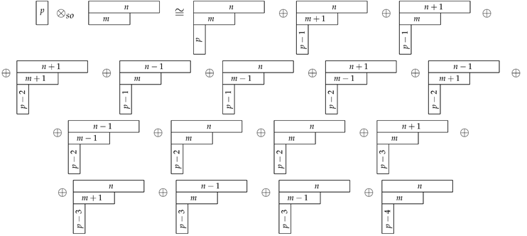
For $1\le p\le 3$, the diagrams carrying negative p-dependent labels are absent. It is important to note that the diagram $(n,m,p-2)$ is present twice: one copy results from the contraction of one of the form indices with the first row followed by the symmetrization of another form index with the same row. Another one results from the application of the same procedure to the second row. This fact leads to two different tensor implementations. Also note that some of the diagrams vanish for special dimensions by virtue of the Two-Column Theorem:

Theorem 2.

$\mathfrak{so}\left(d\right)$ traceless tensors with the symmetry properties of such Young diagrams that the sum of the heights of the first two columns exceeds d, are identically zero [36].

The cohomology $H^p\left({\sigma }_{-}\right)$ is empty for $p>d$. Analogously, some potential elements of $H^p\left({\sigma }_{-}\right)$ are zero by the Two-Column Theorem for large $p\le d$.

Now we are in a position to consider the action of the Laplace operator on each of the diagrams (109) separately. In the following restrictions on $n,m,p$ will be imposed: if for some $n,m,p$ a tensor has a wrong Young shape, it is zero. In most cases we will simplify calculation by demanding p-forms be ${\sigma }_{-}$-closed. Another simplification is due to the fact that $\mathsf{\Delta }F=0$ is equivalent to the two equations ${\sigma }_{-}F=0$ and ${\sigma }_{+}F=0$.

Diagram (n,m;p), $n\ge 0,m\ge 0,p\ge 0$ has the tensor form $T_{a\left(n\right),b\left(m\right),c_1,..,c_p}$. It is ${\sigma }_{-}$-closed, if $m=0$. Then

$$\mathsf{\Delta }{T}_{a\left(n\right),c_1,..,c_p}=p{T}_{a\left(n\right),c_1,..,c_p}.$$

(110)

This diagram is in $ker\left(\mathsf{\Delta }\right)$ at $p=0$ that reproduces the already obtained result for $H^0\left({\sigma }_{-}\right)$.

Diagram (n + 1,m + 1;p − 2), $n\ge 0,m\ge 0,p\ge 2$ has the tensor form $T_{a\left(n\right)c_1,b\left(m\right)c_2,..,c_p}$. This diagram is ${\sigma }_{-}$-closed. The action of $\mathsf{\Delta }$ is

$$\mathsf{\Delta }{T}_{a\left(n\right)c_1,b\left(m\right)c_2,..,c_p}=\frac{(n-m)(p+m-1)}{(n-m+1)}{T}_{a\left(n\right)c_1,b\left(m\right)c_2,..,c_p}.$$

(111)

This diagram is in $ker\left(\mathsf{\Delta }\right)$, if $n=m$, thus belonging to $H^p\left({\sigma }_{-}\right)$ with $p\ge 2$.

Diagram (n,m + 1;p − 1), $n\ge 1,m\ge 0,p\ge 1$ has the tensor form $T_{a\left(n\right),b\left(m\right)c_0,c_1,..,c_{p-1}}$. Then

$$\mathsf{\Delta }{T}_{a\left(n\right),b\left(m\right)c_0,c_1,..,c_{p-1}}=(m+p)T_{a\left(n\right),b\left(m\right)c_0,c_1,..,c_{p-1}}.$$

(112)

This equation admits no solutions since $p\ge 1$ in the case in question.

Diagram (n + 1,m;p − 1), $n\ge 0,m\ge 0,p\ge 1$ has the tensor form

$$T_{a\left(n\right)c_0,b\left(m\right),c_1,..,c_{p-1}}+\frac{m}{n-m+2}{T}_{a\left(n\right)b,b(m-1)c_0,c_1,..,c_{p-1}}.$$

It is ${\sigma }_{-}$-closed iff $m=0$. Then

$$\mathsf{\Delta }{T}_{a\left(n\right)c_0,c_1,..,c_{p-1}}=\frac{n(p-1)}{n+1}{T}_{a\left(n\right)c_0,c_1,..,c_{p-1}}.$$

(113)

This expression vanishes at $p=1$. Hence,

$$T_{a\left(n\right)c_0}\in H^1\left({\sigma }_{-}\right).$$

(114)

As one can see, $n=0$ in (113) also leads to zero Laplace action. However, this is not a new result, since it has been already accounted in the diagrams $(n,m;p)$ for $n=m=p=0$ (110), $(n+1,m+1;p-2)$ for $n=m=0,p\ge 2$ (111) and the $n=m=0,p=1$ case of $(n+1,m;p-1)$ (113). This fact is a simple consequence of the tensor multiplication of a column by a scalar.

Diagram (n − 1,m;p − 1), $n\ge 1,m\ge 0,p\ge 1$ has the tensor form

$$\begin{array}{c}T={\eta }_{a{c}_1}{\rho }_{a(n-1),b\left(m\right),c_2,..,c_p}-\frac{n-1}{d-4+2n}{\eta }_{aa}{\rho }_{a(n-2)c_1,b\left(m\right),c_2,..,c_p}+\frac{m(n-1)}{(d-4+m+n)(d-4+2n)}\hfill \\ \hfill \times {\eta }_{aa}{\rho }_{a(n-2)b,b(m-1)c_1,c_2,..,c_p}-\frac{m}{d-4+m+n}{\eta }_{ab}{\rho }_{a(n-1),b(m-1)c_1,c_2,..,c_p},\end{array}$$

(115)

where $\rho$ is an arbitrary $(n-1,m;p-1)$ tensor.

One can check that $T\in ker\left({\sigma }_{-}\right)$ demands $m=0$ with

$$T={\eta }_{a{c}_1}{\rho }_{a(n-1),c_2,..,c_p}-\frac{n-1}{d-4+2n}{\eta }_{aa}{\rho }_{a(n-2)c_1,c_2,..,c_p}.$$

(116)

After some calculation we obtain

$$\mathsf{\Delta }T=\frac{(p-1)(d-2+n)}{d-3+n}T.$$

(117)

This implies that $\mathsf{\Delta }$ has zero at $p=1$ contributing to $H^1\left({\sigma }_{-}\right)$. The case of $d=2,n=1$ must be considered separately because of the divergent denominator. The seeming divergence emerges due to the second term in (116), which is absent at $d=2,n=1$,

$$T={\eta }_{a{c}_1}{\rho }_{c_2,..,c_p}\Rightarrow {\sigma }_{+}T=\frac{p-1}{2}\left({\eta }_{b{c}_1}{\rho }_{a,c_2,..,c_{p-1}}-{\eta }_{a{c}_1}{\rho }_{b,c_2,..,c_{p-1}}\right),$$

(118)

leading to the same answer with $p=1$.

Diagram (n,m − 1;p − 1) $n\ge 1,m\ge 1,p\ge 1$ has the tensor form

$$\begin{array}{c}T=(n-1){\eta }_{aa}{\rho }_{a(n-2)b{c}_1,b(m-1),c_2,..,c_p}-\frac{(n-1)(m-1)}{d-6+2m}{\eta }_{aa}{\rho }_{a(n-2)bb,b(m-2)c_1,c_2,..,c_p}-(d-4+m+n)\hfill \\ \times {\eta }_{a{c}_1}{\rho }_{a(n-1)b,b(m-1),c_2,..,c_p}-(n-m){\eta }_{ab}{\rho }_{a(n-1)c_1,b(m-1),c_2,..,c_p}+\frac{(m-1)(d-4+2n)}{d-6+2m}{\eta }_{ab}\\ \times {\rho }_{a(n-1)b,b(m-2)c_1,c_2,..,c_p}+\frac{(n-m+1)(d-4+m+n)}{n}{\eta }_{b{c}_1}{\rho }_{a\left(n\right),b(m-1),c_2,..,c_p}\\ \hfill -\frac{(m-1)(n-m+1)(d-4+m+n)}{(d-6+2m)n}{\eta }_{bb}{\rho }_{a\left(n\right),b(m-2)c_1,c_2,..,c_p},\end{array}$$

(119)

where $\rho$ is an arbitrary $(n,m-1;p-1)$ tensor.

Let us show that this diagram can never be annihilated by ${\sigma }_{-}$. Indeed,

$${\sigma }_{-}T= \left(d-4+m+n-(n-m)\right){\eta }_{a{c}_0}{\rho }_{a(n-1)c_1,b(m-1),c_2,..,c_p}+(m-1)\left(lit\right),$$

(120)

where (lit) denotes some terms that are linearly independent from the first one. If $m=1$ the above expression reduces to

$${\sigma }_{-}T= \left(d-2\right){\eta }_{a{c}_0}{\rho }_{a(n-1)c_1,c_2,..,c_p}.$$

(121)

The expression in brackets vanishes at $d=2$. However, such diagram is zero by virtue of the Two-column theorem 2, since the heights of the first two columns sum up to $3>d$.

Thus, the nontrivial T is never in $ker\left({\sigma }_{-}\right)$.

Diagram (n + 1,m − 1;p − 2) $n\ge 1,m\ge 1,p\ge 2$ has the tensor form

$$\begin{array}{c}T={\eta }_{a{c}_1}{\rho }_{a(n-1)b{c}_2,b(m-1),c_3,..c_p}-\frac{n-m+1}{n}{\eta }_{b{c}_1}{\rho }_{a\left(n\right)c_2,b(m-1),c_3,..c_p}\hfill \\ +\frac{m-1}{n-m+3}{\eta }_{a{c}_1}{\rho }_{a(n-1)bb,b(m-2)c_2,c_3,..c_p}-\frac{(m-1)(n-1)}{(d-6+2m)(n-m+3)}{\eta }_{aa}{\rho }_{a(n-2)bb{c}_1,b(m-2)c_2,c_3,..c_p}\\ +\frac{2(m-1)(n-m+1)}{(d-6+2m)(n-m+3)}{\eta }_{ab}{\rho }_{a(n-1)b{c}_1,b(m-2)c_2,c_3,..c_p}-\frac{(m-1)(n-m+1)}{n(n-m+3)}\\ \hfill \times {\eta }_{b{c}_1}{\rho }_{a\left(n\right)b,b(m-2)c_2,c_3,..c_p}-\frac{(m-1)(n-m+2)(n-m+1)}{(d-6+2m)(n-m+3)n}{\eta }_{bb}{\rho }_{a\left(n\right)c_1,b(m-2)c_2,c_3,..c_p},\end{array}$$

(122)

where $\rho$ is an arbitrary $(n+1,m-1;p-2)$ tensor.

Though the tensor realization (122) may look complicated, the problem is simplified by the observation that all terms except for the first and second ones carry a factor of $(m-1)$. The action of ${\sigma }_{-}$ on the first and second terms produces a factor of $(m-1)$ in front of each $\eta \rho$ combination. It can be checked that ${\sigma }_{-}T$ has an overall factor of $(m-1)$ so that the only possible solution for $T\in ker\left({\sigma }_{-}\right)$ is at $m=1$ in which case the tensor decomposition acquires the form

$$T={\eta }_{a{c}_1}{\rho }_{a(n-1)b{c}_2,..,c_p}-{\eta }_{b{c}_1}{\rho }_{a\left(n\right)c_2,..,c_p}.$$

(123)

At $p=2$, after some calculations one can check that

$${\sigma }_{+}T=0.$$

(124)

For $p>2$ it is not difficult to see that ${\sigma }_{+}T\ne 0$. Indeed,

$${\sigma }_{+}T=(p-2)\left(1+\frac{1}{n}\right){\eta }_{a{c}_1}{\rho }_{a(n-1)b{c}_2,b,c_3,..,c_{p-1}}+\left(lit\right),$$

(125)

where (lit) denotes other linearly independent terms. The first term is never zero.

Thus,

$$T={\eta }_{a{c}_1}{\rho }_{a(n-1)b{c}_2}-{\eta }_{b{c}_1}{\rho }_{a\left(n\right)c_2}\in H^2\left({\sigma }_{-}\right).$$

(126)

Diagram (n − 1,m + 1;p − 2), $n\ge 1,m\ge 0,p\ge 2$ has the tensor form

$$T={\eta }_{a{c}_1}{\rho }_{a(n-1),b\left(m\right)c_2,..,c_p}-\frac{n-1}{d-4+2n}{\eta }_{aa}{\rho }_{a(n-2)c_1,b\left(m\right)c_2,..,c_p},$$

(127)

where $\rho$ is an arbitrary $(n-1,m+1;p-2)$ tensor.

Though it is obviously in $ker\left({\sigma }_{-}\right)$ for any m, it is not hard to see that it is never in $ker\left({\sigma }_{+}\right)$.

$${\sigma }_{+}T=-\left(1+\frac{p-2}{m+1}\right){\eta }_{a{c}_1}{\rho }_{a(n-1),b(m+1),..,c_{p-1}}+\left(lit\right).$$

(128)

Hence this diagram does not contribute to $H^p\left({\sigma }_{-}\right)$.

Diagram (n − 1,m − 1;p − 2), $n\ge 1,m\ge 1,p\ge 2$ has an involved tensor form. Since the coefficients in the expression below are complicated, we extract the factor of $(m-1)$ once present denoting the leftover coefficients as ${\alpha }_i$,

$$\begin{array}{c}T={\eta }_{a{c}_1}{\eta }_{b{c}_2}{\rho }_{a(n-1),b(m-1),..,c_p}+(m-1){\alpha }_1{\eta }_{aa}{\eta }_{aa}{\rho }_{a(n-4)bb{c}_1,b(m-2)c_2,..,c_p}\hfill \\ + {\alpha }_2{\eta }_{aa}{\eta }_{a{c}_1}{\rho }_{a(n-3)b{c}_2,b(m-1),..,c_p}+(m-1){\alpha }_3{\eta }_{aa}{\eta }_{a{c}_1}{\rho }_{a(n-3)bb,b(m-2)c_2,..,c_p}\\ +(m-1){\alpha }_4{\eta }_{aa}{\eta }_{ab}{\rho }_{a(n-3)b{c}_1,b(m-2)c_2,..,c_p}+{\alpha }_5{\eta }_{aa}{\eta }_{b{c}_1}{\rho }_{a(n-2)c_2,b(m-1),..,c_p}\\ +(m-1){\alpha }_6{\eta }_{aa}{\eta }_{b{c}_1}{\rho }_{a(n-2)b,b(m-2)c_2,..,c_p}+(m-1){\alpha }_7{\eta }_{aa}{\eta }_{bb}{\rho }_{a(n-2)c_1,b(m-2)c_2,..,c_p}\\ + {\alpha }_8{\eta }_{a{c}_1}{\eta }_{ab}{\rho }_{a(n-2)c_2,b(m-1),..,c_p}+(m-1){\alpha }_9{\eta }_{a{c}_1}{\eta }_{ab}{\rho }_{a(n-2)b,b(m-2)c_2,..,c_p}\\ +(m-1){\alpha }_{10}{\eta }_{a{c}_1}{\eta }_{bb}{\rho }_{a(n-1),b(m-2)c_2,..,c_p}+(m-1){\alpha }_{11}{\eta }_{ab}{\eta }_{ab}{\rho }_{a(n-2)c_1,b(m-2)c_2,..,c_p}\\ \hfill +(m-1){\alpha }_{12}{\eta }_{ab}{\eta }_{b{c}_1}{\rho }_{a(n-1),b(m-2)c_2,..,c_p},\end{array}$$

(129)

where $\rho$ is an arbitrary $(n-1,m-1;p-2)$ tensor. The explicit form of ${\alpha }_i$ is given in the Appendix A.

Now we observe that the action of ${\sigma }_{-}$ on the terms free of the factor of $(m-1)$ produces such factor. Hence, ${\sigma }_{-}\left(T\right)$ has the form of the sum of linearly independent terms with the common factor of $(m-1)$. Consequently,

$${\sigma }_{-}T=0,\mathrm{iff}m=1.$$

(130)

At $m=1$, the only terms that remain are

$$\begin{array}{c}T={\eta }_{a{c}_1}{\eta }_{b{c}_2}{\rho }_{a(n-1),..,c_p}+\frac{(n-2)(n-1)}{(d-3+n)(d-4+2n)}{\eta }_{aa}{\eta }_{a{c}_1}{\rho }_{a(n-3)b{c}_2,..,c_p}\hfill \\ \hfill +\frac{(n-1)(d-2+n)}{(d-3+n)(d-4+2n)}{\eta }_{aa}{\eta }_{b{c}_1}{\rho }_{a(n-2)c_2,..,c_p}-\frac{n-1}{d-3+n}{\eta }_{a{c}_1}{\eta }_{ab}{\rho }_{a(n-2)c_2,..,c_p}.\end{array}$$

(131)

It can be checked that for $p=2$

$${\sigma }_{+}T=0.$$

(132)

For $p>2$ it is not difficult to see that

$${\sigma }_{+}T=\frac{(p-2)d}{(d-2)(d-3+n)(d-2+n)}{e}_3^2{\theta }_Y\rho +\left(lit\right),$$

(133)

where $\rho ={\rho }_{a(n-1),c_1,..,c_{p-2}}{Y}^{a(n-1)}{\theta }^{c_1}..{\theta }^{c_{p-2}}$. Therefore,

$$\begin{array}{c}{H}^2\left({\sigma }_{-}\right)\ni T={\eta }_{a{c}_1}{\eta }_{b{c}_2}{\rho }_{a(n-1)}+\frac{(n-2)(n-1)}{(d-3+n)(d-4+2n)}{\eta }_{aa}{\eta }_{a{c}_1}{\rho }_{a(n-3)b{c}_2}\hfill \\ \hfill +\frac{(n-1)(d-2+n)}{(d-3+n)(d-4+2n)}{\eta }_{aa}{\eta }_{b{c}_1}{\rho }_{a(n-2)c_2}-\frac{n-1}{d-3+n}{\eta }_{a{c}_1}{\eta }_{ab}{\rho }_{a(n-2)c_2}.\end{array}$$

(134)

Diagram (n + 1,m;p − 3), $n\ge 1,m\ge 1,p\ge 3$ has the tensor form

$$T={\eta }_{b{c}_1}{\rho }_{a\left(n\right)c_2,b(m-1)c_3,..,c_p}-\frac{n}{n-m+1}{\eta }_{a{c}_1}{\rho }_{a(n-1)b{c}_2,b(m-1)c_3,..,c_p},$$

(135)

where $\rho$ is an arbitrary $(n+1,m;p-3)$ tensor.

Explicit computation gives

$$\begin{array}{c}\mathsf{\Delta }T=\frac{t_0}{t_0+1}\left(p+h_2-1\right)T-\frac{2t_0}{(t_0+1)(d-4+2h_2)}{\theta }^a{Z}_a{\partial }_{\theta Z}T\hfill \\ + \frac{d-4+2h_1}{(t_0+1)(d-3+h_1+h_2)(d-4+2h_2)}\left(t_2{\theta }^a{Y}_a{\partial }_{\theta Z}-{\theta }^a{Z}_a{\partial }_{\theta Z}\right)T\\ -\frac{t_0-1}{(t_0+1)(d-3+h_1+h_2)}{\theta }^a{Y}_a{\partial }_{\theta Y}T.\hfill \end{array}$$

(136)

This expression vanishes at $n=m$. Indeed, in this case $t_{0}T=0,h_{1}T=h_{2}T=nT,t_{2}T=0$ so that

$$\mathsf{\Delta }T=\frac{1}{d-3+2n}\left(t_2{\theta }^a{Y}_a{\partial }_{\theta Z}-{\theta }^a{Z}_a{\partial }_{\theta Z}\right)T+\frac{1}{d-3+2n}{\theta }^a{Y}_a{\partial }_{\theta Y}T.$$

(137)

Since

$$t_2{\theta }^a{Y}_a{\partial }_{\theta Z}T={\theta }^a{Y}_a{\partial }_{\theta Z}{t}_{2}T-{\theta }^a{Y}_a{\partial }_{\theta Y}T+{\theta }^a{Z}_a{\partial }_{\theta Z}T=-{\theta }^a{Y}_a{\partial }_{\theta Y}T+{\theta }^a{Z}_a{\partial }_{\theta Z}T,$$

(138)

it follows that $\mathsf{\Delta }T=0$ at $n=m$. To check that $\mathsf{\Delta }T\ne 0$ at $n\ne m$ one should substitute the expression for T noticing that different linearly independent terms have no common factor to vanish, that implies nontriviality of $\mathsf{\Delta }T$.

Diagram (n,m + 1;p − 3), $n\ge 1,m\ge 0,p\ge 3$ has the tensor form $T={\eta }_{a{c}_1}{\rho }_{a(n-1)c_2,b\left(m\right)c_3,..,c_p}$. It belongs to $ker\left({\sigma }_{-}\right)$, but not to $ker\left({\sigma }_{+}\right)$.

$${\sigma }_{+}T= \left(1+\frac{p-3}{m+1}\right){\eta }_{a{c}_1}{\rho }_{a(n-1)c_2,b(m+1),..,c_p}+\left(lit\right).$$

(139)

Diagram (n,m;p − 2) $n\ge 1,m\ge 0,p\ge 2$ admits two tensor realizations $T_i$ due to the double presence of this diagram in the result of tensor product. The tensors

$$T_1={\eta }_{a{c}_1}{{\rho }_1}_{a(n-1)c_2,b\left(m\right),c_3,..,c_p}+\frac{m}{n}{\eta }_{b{c}_1}{{\rho }_1}_{a\left(n\right),b(m-1)c_2,c_3,..,c_p},$$

(140)

$$\begin{array}{c}{T}_2={\eta }_{aa}{{\rho }_2}_{a(n-2)b{c}_1,b(m-1)c_2,c_3,..,c_p}-\frac{n-m}{n-1}{\eta }_{ab}{{\rho }_2}_{a(n-1)c_1,b(m-1)c_2,c_3,..,c_p}-\frac{d-4+n+m}{n-1}{\eta }_{a{c}_1}\hfill \\ \hfill \times {{\rho }_2}_{a(n-1)b,b(m-1)c_2,c_3,..,c_p}+\frac{(n-m+1)(d-4+m+n)}{n(n-1)}{\eta }_{b{c}_1}{{\rho }_2}_{a\left(n\right),b(m-1)c_2,c_3,..,c_p}\end{array}$$

(141)

are linearly independent. That Laplace operator acts diagonally on $T_i$, $\mathsf{\Delta }{T}_i={\lambda }_i(n,m,p)T_i$, allows us to separately consider each of these diagrams. Firstly, we check if these are in $ker\left({\sigma }_{-}\right)$ computing

$$\begin{array}{cc}\hfill & {\sigma }_{-}{T}_1=m{\eta }_{a{c}_1}{{\rho }_1}_{a(n-1)c_2,b(m-1)c_3,..,c_{p+1}},\hfill \end{array}$$

(142)

$$\begin{array}{cc}\hfill & {\sigma }_{-}{T}_2=\frac{d-4+2m}{n-1}{\eta }_{a{c}_1}{{\rho }_2}_{a(n-1)c_2,b(m-1)c_3,..,c_{p+1}}.\hfill \end{array}$$

(143)

$T_1\in ker\left({\sigma }_{-}\right)$ at $m=0$. Formally, $T_2$ is annihilated by ${\sigma }_{-}$ at $d=2,m=1$, but this is not allowed by the Two-column theorem. So, the only candidate for cohomology is $T_1$. However,

$${\sigma }_{+}{T}_1=\frac{1}{n+1}\left(1+\frac{p-2}{n}\right){\eta }_{b{c}_1}{{\rho }_1}_{a\left(n\right),c_2,..,c_{p-1}}+\left(lit\right),$$

(144)

which is never zero.

Diagram (n−1,m;p−3), $n\ge 2,m\ge 1,p\ge 3$ has the tensor form

$$\begin{array}{c}T={\eta }_{a{c}_1}{\eta }_{b{c}_2}{\rho }_{a(n-1),b(m-1)c_3,..,c_p}-\frac{(n-1)(d-3+m+n)}{(d-4+n+m)(d-4+2n)}{\eta }_{aa}{\eta }_{b{c}_1}{\rho }_{a(n-2)c_2,b(m-1)c_3,..,c_p}\hfill \\ -\frac{(n-1)(n-2)}{(d-4+m+n)(d-4+2n)}{\eta }_{aa}{\eta }_{a{c}_1}{\rho }_{a(n-3)b{c}_2,b(m-1)c_3,..,c_p}+\frac{n-1}{d-4+m+n}\\ \times {\eta }_{ab}{\eta }_{a{c}_1}{\rho }_{a(n-2)c_2,b(m-1)c_3,..,c_p},\hfill \end{array}$$

(145)

where $\rho$ is an arbitrary $(n-1,m;p-3)$ tensor.

Obviously, $T\in ker\left({\sigma }_{-}\right)$. However, $T\notin ker\left({\sigma }_{+}\right)$.

$${\sigma }_{+}T=\left(1+\frac{p-3}{m}\right){\eta }_{a{c}_1}{\eta }_{b{c}_2}{\rho }_{a(n-1),b\left(m\right),c_3,..,c_{p-1}}+\left(lit\right),$$

(146)

hence not contributing to cohomology.

Diagram (n,m−1;p−3), $n\ge 1,m\ge 1,p\ge 3$ has the tensor form

$$T={\eta }_{a{c}_1}{\eta }_{b{c}_2}{\rho }_{a(n-1)c_3,b(m-1),..,c_p}+(m-1)\left(lit\right)$$

(147)

with all terms except for the first one carrying a factor of $(m-1)$. The action of ${\sigma }_{-}$ on the first term brings a factor of $(m-1)$ in front of $\eta \rho$. Since all $\eta \rho$ terms in the decomposition are linearly independent we conclude that

$${\sigma }_{-}T=0,\mathrm{if}m=1.$$

(148)

At $p=3$ one can check that ${\sigma }_{+}T=0$. However, for $p>3$ T does not belong to $ker\left({\sigma }_{+}\right)$,

$${\sigma }_{+}T=-(p-3){\eta }_{a{c}_1}{\eta }_{b{c}_2}{\rho }_{a(n-1)c_3,b,..,c_{p-1}} + \left(lit\right).$$

(149)

Consequently, the only contribution to $H^3\left({\sigma }_{-}\right)$ is

$$T={\eta }_{a{c}_1}{\eta }_{b{c}_2}{\rho }_{a(n-1)c_3}\in H^3\left({\sigma }_{-}\right).$$

(150)

Diagram (n,m;p−4), $n\ge 1,m\ge 1,p\ge 4$ has the tensor form

$$T={\eta }_{a{c}_1}{\eta }_{b{c}_2}{\rho }_{a(n-1)c_3,b(m-1)c_4,..,c_p}.$$

(151)

This is obviously annihilated by ${\sigma }_{-}$, but not by ${\sigma }_{+}$.

$${\sigma }_{+}T=-\left(1+\frac{p-4}{m}\right){\eta }_{a{c}_1}{\eta }_{b{c}_2}{\rho }_{a(n-1)c_3,b\left(m\right),..,c_{p-1}}+\left(lit\right).$$

(152)

Hence it does not contribute to $H^p\left({\sigma }_{-}\right)$.

5.3.5. Summary

Summarizing the results of Section 5.3.3 and Section 5.3.4 we found the following cohomology groups:

$$H^0\left({\sigma }_{-}\right)=\{F=F_{a\left(n\right)}{Y}^{a\left(n\right)}|F\in V^0\},$$

(153)

$$\begin{array}{c}{H}^1\left({\sigma }_{-}\right)=\{\varphi ={F_1}_{a\left(n\right)c}{Y}^{a\left(n\right)}{\theta }^c,F_1\in V^1;\hfill \\ {\varphi }^{tr}= \left[(n-1){\eta }_{aa}{F_2}_{a(n-2)c}-(d-4+2n){\eta }_{ac}{F_2}_{a(n-1)}\right]Y^{a\left(n\right)}{\theta }^c\in V^1\},\hfill \end{array}$$

(154)

$$\begin{array}{c}{H}^2\left({\sigma }_{-}\right)=\{W={\theta }_Y{\theta }_{Z}C(Y,Z):t_{0}C=0,C\in V^0;\hfill \\ {\mathcal{E}}_A= \left[{\eta }_{a{c}_1}{{\rho }_1}_{a(n-1)b{c}_2}-{\eta }_{b{c}_1}{{\rho }_1}_{a\left(n\right)c_2}\right]Y^{a\left(n\right)}{Z}^b{\theta }^{c_1}{\theta }^{c_2}\in V^2;\\ {\mathcal{E}}_B=[{\eta }_{a{c}_1}{\eta }_{b{c}_2}{{\rho }_2}_{a(n-1)}+\frac{(n-2)(n-1)}{(d-3+n)(d-4+2n)}{\eta }_{aa}{\eta }_{a{c}_1}{{\rho }_2}_{a(n-3)b{c}_2}\\ \hfill +\frac{(n-1)(d-2+n)}{(d-3+n)(d-4+2n)}{\eta }_{aa}{\eta }_{b{c}_1}{{\rho }_2}_{a(n-2)c_2}-\frac{n-1}{d-3+n}{\eta }_{a{c}_1}{\eta }_{ab}{{\rho }_2}_{a(n-2)c_2}]Y^{a\left(n\right)}{Z}^b{\theta }^{c_1}{\theta }^{c_2}\in V^2\},\end{array}$$

(155)

$$\begin{array}{c}{H}^3\left({\sigma }_{-}\right)=\{B^{fr}={\eta }_{a{c}_1}{\eta }_{b{c}_2}{\rho }_{a(n-1)c_3}{Y}^{a\left(n\right)}{Z}^b{\theta }^{c_1}{\theta }^{c_2}{\theta }^{c_3}\in V^3;\hfill \\ B_1={\theta }_Y{\theta }_{Z}C(Y,Z,\theta ):t_{0}C=0,C=C_{a\left(n\right),b\left(n\right),c}{Y}^{a\left(n\right)}{Z}^{b\left(n\right)}{\theta }^c\in V^1;\\ B_2= \left[{\eta }_{b{c}_1}{\rho }_{a\left(n\right)c_2,b(n-1)c_3}-n{\eta }_{a{c}_1}{\rho }_{a(n-1)b{c}_2,b(n-1)c_3}\right]Y^{a\left(n\right)}{Z}^{b\left(n\right)}{\theta }^{c_1}{\theta }^{c_2}{\theta }^{c_3}\in V^3\}.\hfill \end{array}$$

(156)

At $p>3$

$$\begin{array}{c}{H}^p\left({\sigma }_{-}\right)=\{B_1={\theta }_Y{\theta }_{Z}C(Y,Z,\theta ):t_{0}C=0,C=C_{a\left(n\right),b\left(n\right),c_1,..,c_{p-2}}{Y}^{a\left(n\right)}{Z}^{b\left(n\right)}{\theta }^{c_1}..{\theta }^{c_{p-2}}\in V^{p-2};\hfill \\ \hfill B_2=\left[{\eta }_{b{c}_1}{\rho }_{a\left(n\right)c_2,b(n-1)c_3,..,c_p}-n{\eta }_{a{c}_1}{\rho }_{a(n-1)b{c}_2,b(n-1)c_3,..,c_p}\right]Y^{a\left(n\right)}{Z}^{b\left(n\right)}{\theta }^{c_1}..{\theta }^{c_p}\in V^p\}.\end{array}$$

(157)

According to Theorem 1, the differential gauge transformation parameters are described by $H^0\left({\sigma }_{-}\right)$ (153). The gauge parameter in the Fronsdal theory is known to be a symmetric traceless tensor. Since tensors $(n,0,0)$ constitute the cohomology group $H^0\left({\sigma }_{-}\right)$, the unfolded differential gauge transformation is shown to coincide with the Fronsdal one.

As recalled in Section 2.1, the Fronsdal field consists of two symmetric traceless fields (2). These fields are represented by the cohomology groups $H^1\left({\sigma }_{-}\right)$ (154). Cohomology group $H^1\left({\sigma }_{-}\right)$ consists of two elements $(n+1,0,0)$ and $(n-1,0,0)$ matching the components of the Fronsdal field. Thus, the physical fields in the unfolded approach indeed coincide with the Fronsdal field.

The cohomology group $H^2\left({\sigma }_{-}\right)$ (155) describes gauge invariant combinations of derivatives of the physical fields that can be used to impose differential equations on the latter. The Fronsdal cohomology classes ${\mathcal{E}}_A$ and ${\mathcal{E}}_B$ match with the Fronsdal equations: ${\mathcal{E}}_A$ is associated with the traceless part of the Fronsdal equations, while ${\mathcal{E}}_B$ with the trace part, that is the equations ${\mathcal{E}}_A=0,{\mathcal{E}}_B=0$ just reproduce the Fronsdal equations. Note that the number of resulting equations is the same as the number of fields, as it should be in a Lagrangian system.

W in (155) represents "Weyl" cohomology. Imposing $W=0$ in the case of gravity one gets conformally flat metrics and in the case of higher spins “conformally flat” fields. In Einstein gravity and HS theory, the equation $W=0$ is not imposed. Instead, elements of W are interpreted as new fields C that describe generalized Weyl tensors by virtue of the unfolded Equation (14). Thus, calculation of the cohomology group $H^2\left({\sigma }_{-}\right)$ shows that unfolded Equations (13) and (14) contain Fronsdal equations along with constraints on auxiliary fields.

In accordance with the general discussion of Section 3 elements of $H^3\left({\sigma }_{-}\right)$ (156) correspond to Bianchi identities. Class $B^{fr}$ describes the Bianchi identities for the Fronsdal equations. Note that their number coincides with the number of differential gauge parameters. The remaining classes $B_1$ and $B_2$ correspond to the Bianchi identities on the Weyl tensor. It is noteworthy that the latter can be checked to coincide with the first ${\tilde{\sigma }}_{-}$ cohomology in the Weyl sector of zero-forms of [10] for $s>1$. This fact exhibits the connection between the gauge and Weyl sectors.

For $p>3$ cohomology groups $H^p\left({\sigma }_{-}\right)$ describe the higher Bianchi identities for Bianchi identities on the Weyl tensor also interpreted as syzygies [24].

Obtained lower cohomology groups match with the results of [16,17,18].

In HS theory the fields are realized by one-forms. Formally, one can consider field Equations (13) and (14) for p-forms ${\omega }_{a\left(n\right),b\left(m\right)}$ valued in a two-row irreducible $\mathfrak{o}\left(d\right)$-module. From our results and physical interpretation of the ${\sigma }_{-}$ cohomology groups it follows that for $p>1$ the unfolded system in the gauge sector is off-shell. To answer the question whether the full unfolded system including both the gauge p-form sector and the Weyl $(p-1)$-form sector is off-shell, the analysis of $H\left({\tilde{\sigma }}_{-}\right)$ has to be performed in the Weyl sector. The case of $p>1$ may be somewhat similar to the $s=1$ case, where the equation on $A_{\mu }$ lies in the Weyl sector.

Finally, let us stress that the results of this section for HS fields in Minkowski space admit a straightforward deformation to $Ad{S}_d$ with the same operator ${\sigma }_{-}$. This is because in that case dynamical fields are described by rectangular diagrams of the $Ad{S}_d$ algebra $\mathfrak{o}(d-1,2)$ [37]. In general, in the flat limit, irreducible massless (gauge) fields in $Ad{S}_d$ decompose into nontrivial sets of irreducible flat space massless fields [38,39,40] and there is no one-to-one correspondence between massless fields in Minkowski space and $Ad{S}_d$. Namely, a generic irreducible field in Minkowski space may admit no deformation to $Ad{S}_d$ (see also [41]).

6. ${\mathbf{\sigma }}_{-}$ Cohomology in $\mathit{A}\mathit{d}{\mathit{S}}_{\mathbf{4}}$ in the Spinor Language

$4d$ HS theories admit a description in terms of two-component spinors instead of tensors. That is, instead of using the generating functions in the tensor form $\omega (x,dx|Y,Z)$, where $Y^a$ and $Z^a$ carried vector Lorentz indices $a=\{0,1,2,3\}$, we will use

$$\omega (y,\overline{y}|x,dx)=\sum _{k,m}{\omega }^{{\alpha }_1\dots {\alpha }_k,{\dot{\alpha }}_1\dots {\dot{\alpha }}_m}(x,dx)y_{{\alpha }_1}\dots y_{{\alpha }_k}{\overline{y}}_{{\dot{\alpha }}_1}\dots {\overline{y}}_{{\dot{\alpha }}_m},$$

(158)

where the indices $\alpha$ and $\dot{\alpha }$ of the two-component commuting spinors $y^{\alpha }$ and ${\overline{y}}^{\dot{\alpha }}$ take two values $\{1,2\}$.

Analogously to Section 3 and Section 4, we have to introduce the grading on the space of ${\mathsf{\Lambda }}^{•}\left(M\right)\otimes \mathbb{C}\left[[y,\overline{y}]\right]$. Consider the homogeneous element of ${\mathsf{\Lambda }}^{•}\left(M\right)\otimes \mathbb{C}\left[[y,\overline{y}]\right]$ of degree N and $\overline{N}$ in y and $\overline{y}$, respectively

$$\omega (\mu y,\overline{\mu y}|x,dx)={\mu }^N{\overline{\mu }}^{\overline{N}}\omega (y,\overline{y}|x,dx).$$

(159)

Define the grading operator G on ${\mathsf{\Lambda }}^{•}\left(M\right)\otimes \mathbb{C}\left[[y,\overline{y}]\right]$ as follows:

$$G\omega (y,\overline{y}|x,dx)=|N-\overline{N}|\omega (y,\overline{y}|x,dx)\equiv |{deg}_y\left(\omega (y,\overline{y}|x,dx)\right)-{deg}_{\overline{y}}\left(\omega (y,\overline{y}|x,dx)\right)|.$$

(160)

Note that in the bosonic sector the frame-like fields $e^{m_1\dots m_{s-1}}\leftrightarrow e^{{\alpha }_1\dots {\alpha }_{s-1},{\dot{\alpha }}_1\dots {\dot{\alpha }}_{s-1}}$ have the lowest possible grading $G=0$. For our later computations to match with the Fronsdal theory, we define the action of ${\sigma }_{-}$ on $\omega (y,\overline{y})$ to decrease the G-grading:

$$\begin{array}{cc}\hfill {\sigma }_{-}\omega (y,\overline{y})& :=i{\overline{y}}^{\dot{\alpha }}{h}_{\dot{\alpha }}^{\alpha }{\partial }_{\alpha }\omega (y,\overline{y}),\mathrm{at}{deg}_y\left(\omega \right)>{deg}_{\overline{y}}\left(\omega \right),\hfill \end{array}$$

(161a)

$$\begin{array}{cc}\hfill {\sigma }_{-}\omega (y,\overline{y})& :=i{y}^{\alpha }{h}_{\alpha }^{\dot{\alpha }}{\overline{\partial }}_{\dot{\alpha }}\omega (y,\overline{y}),\mathrm{at}{deg}_y\left(\omega \right)<{deg}_{\overline{y}}\left(\omega \right),\hfill \end{array}$$

(161b)

$$\begin{array}{cc}\hfill {\sigma }_{-}\omega (y,\overline{y})& :=0\mathrm{at}{deg}_y\left(\omega \right)={deg}_{\overline{y}}\left(\omega \right),\hfill \end{array}$$

(161c)

where

$$\begin{array}{c}\hfill {\partial }_{\alpha }:=\frac{\partial }{\partial y^{\alpha }},{\overline{\partial }}_{\dot{\alpha }}:=\frac{\partial }{\partial {\overline{y}}^{\dot{\alpha }}},\end{array}$$

(162)

and the dependence on x and $dx$ in $\omega (y,\overline{y})=\omega (y,\overline{y}|x,dx)$ is always implicit.

It is easy to check that so defined ${\sigma }_{-}$ is nilpotent, ${\left({\sigma }_{-}\right)}^2=0$.

Note that ${\sigma }_{\pm }$ change the grading G by 2. This agrees in particular with the fact that the bosonic and fermionic sectors, where the grading is even and odd respectively, are independent. We consider in detail the more complicated bosonic case, observing in the end that the computation for fermionic fields is quite similar.

Note that the analysis of ${\sigma }_{-}$ cohomology in the $4d$ conformal HS theory was also performed in terms of two-component spinors in [42,43]. It is more complicated since the generating functions of conformal HS theory depend on twice as many independent spinors, but simpler since it is free of the module factors like $|N-N|$ in the grading definition (160).

Next, we define a scalar product (Being $\mathrm{SL}(2,\mathbb{C})$-invariant this scalar product is not positive-definite. Analogously to the tensorial case, without affecting the ${\sigma }_{-}$ cohomology analysis it can be made positive-definite by going to the $\mathfrak{su}\left(2\right)\oplus \mathfrak{su}\left(2\right)$ algebra, which is the compact real form of $\mathfrak{sl}(2,\mathbb{C})\oplus \mathfrak{sl}(2,\mathbb{C})$ with altered conjugation rules ${\overline{y}}^{\alpha }=y_{\alpha }$, ${\overline{y}}^{\dot{\alpha }}=y_{\dot{\alpha }}$.) on generating elements of ${\mathsf{\Lambda }}^{•}\left(M\right)\otimes \mathbb{C}\left[[y,\overline{y}]\right]$ by

$$\begin{array}{ccccc}\hfill ⟨q^{\alpha }|q^{\beta }⟩=⟨y^{\alpha }|y^{\beta }⟩=i{ϵ}^{\alpha \beta },& \hfill & \hfill ⟨{\overline{p}}_{\dot{\alpha }}|{\overline{p}}_{\dot{\beta }}⟩=-⟨{\overline{\partial }}_{\dot{\alpha }}|{\overline{\partial }}_{\dot{\beta }}⟩=i{\overline{ϵ}}_{\dot{\alpha }\dot{\beta }},& \hfill & \hfill ⟨h_{\alpha \dot{\alpha }}|h_{\beta \dot{\beta }}⟩={ϵ}_{\alpha \beta }{ϵ}_{\dot{\alpha }\dot{\beta }},\end{array}$$

(163)

where $q^{\alpha }=y^{\alpha }$, $p_{\alpha }=i{\partial }_{\alpha }$ and $h^{\alpha \dot{\beta }}$ is a vierbein one-form.

In some local coordinates $x^{\mu }$ on the base manifold (which in our case is $Ad{S}_4$) the vierbein one-forms $h_{\dot{\alpha }}^{\alpha }$ can be expressed as

$$h_{\dot{\alpha }}^{\alpha }={\left(h_{\mu }\right)}_{\dot{\alpha }}^{\alpha }d{x}^{\mu }.$$

(164)

The $Ad{S}_4$ vierbein ${\left(h_{\mu }\right)}_{\dot{\alpha }}^{\alpha }$ is demanded to be non-degenerate at any point of $Ad{S}_4$.

The next step is to obtain ${\sigma }_{+}:={\sigma }_{-}^{†}$ with respect to the scalar product $⟨,⟩$, i.e., $⟨\varphi |{\sigma }_{-}\psi ⟩=⟨{\sigma }_{+}\varphi |\psi ⟩$. It is not hard to check that

$$\begin{array}{cc}\hfill {\sigma }_{+}\omega (y,\overline{y})& :=-i{y}^{\alpha }{D}_{\alpha }^{\dot{\alpha }}{\overline{\partial }}_{\dot{\alpha }}\omega (y,\overline{y})\mathrm{at}{deg}_y\left(\omega \right)>{deg}_{\overline{y}}\left(\omega \right),\hfill \end{array}$$

(165a)

$$\begin{array}{cc}\hfill {\sigma }_{+}\omega (y,\overline{y})& :=-i{\overline{y}}^{\dot{\alpha }}{D}_{\dot{\alpha }}^{\alpha }{\partial }_{\alpha }\omega (y,\overline{y})\mathrm{at}{deg}_y\left(\omega \right)<{deg}_{\overline{y}}\left(\omega \right),\hfill \end{array}$$

(165b)

$$\begin{array}{cc}\hfill {\sigma }_{+}\omega (y,\overline{y})& :=-i\left(y^{\alpha }{D}_{\alpha }^{\dot{\alpha }}{\overline{\partial }}_{\dot{\alpha }}+{\overline{y}}^{\dot{\alpha }}{D}_{\dot{\alpha }}^{\alpha }{\partial }_{\alpha }\right)\omega (y,\overline{y})\mathrm{at}{deg}_y\left(\omega \right)={deg}_{\overline{y}}\left(\omega \right),\hfill \end{array}$$

(165c)

where

$$\begin{array}{c}\hfill D_{\alpha }^{\dot{\alpha }}:= \frac{\partial }{\partial h_{\dot{\alpha }}^{\alpha }},D_{\dot{\alpha }}^{\alpha }:= \frac{\partial }{\partial h_{\alpha }^{\dot{\alpha }}}.\end{array}$$

(166)

By $\omega =\omega (y,\overline{y}|x,h)$ we mean a general p-form polynomial in y and $\overline{y}$ with the coordinate one-forms $dx$ replaced by h via (164), that is

$$\omega (y,\overline{y}|x,h)=\sum _{n,m}{\omega }_{{\alpha }_1\dots {\alpha }_p\left|\mu \left(n\right)\right|{\dot{\alpha }}_1\dots {\dot{\alpha }}_p|\dot{\mu }\left(m\right)}\left(x\right)h^{{\alpha }_1{\dot{\alpha }}_1}\wedge \cdots \wedge h^{{\alpha }_p{\dot{\alpha }}_p}{y}^{\mu \left(n\right)}{\overline{y}}^{\dot{\mu }\left(m\right)}.$$

(167)

So defined ${\sigma }_{+}$ increases the grading. The Laplace operator

$$\mathsf{\Delta }:={\sigma }_{-}{\sigma }_{+}+{\sigma }_{+}{\sigma }_{-}$$

(168)

is by construction self-adjoint with respect to $⟨|⟩$ and non-negative definite for the compact version of the space-time symmetry algebra.

7. Bosonic Case in ${\mathit{AdS}}_{\mathbf{4}}$

To calculate cohomology of ${\sigma }_{-}$ we have to compute the action of $\mathsf{\Delta }$. Since ${\sigma }_{-}$ and ${\sigma }_{+}$ are defined differently in the different regions of the $(N,\overline{N})$ plane, we compute the Laplacian action in the these regions separately. Direct computation yields:

$$\begin{array}{cc}\hfill {\mathsf{\Delta }}_{N>\overline{N}+2}& =N(\overline{N}+2)+y^{\beta }{\partial }_{\alpha }{h}_{\dot{\gamma }}^{\alpha }{D}_{\beta }^{\dot{\gamma }}+{\overline{y}}^{\dot{\alpha }}{\overline{\partial }}_{\dot{\beta }}{h}_{\gamma \dot{\alpha }}{D}^{\gamma \dot{\beta }},\hfill \end{array}$$

(169a)

$$\begin{array}{cc}\hfill {\mathsf{\Delta }}_{N<\overline{N}-2}& =\overline{N}(N+2)+y^{\alpha }{\partial }_{\beta }{h}_{\alpha \dot{\gamma }}{D}^{\beta \dot{\gamma }}+{\overline{y}}^{\dot{\alpha }}{\overline{\partial }}_{\dot{\beta }}{h}_{\gamma }^{\dot{\beta }}{D}_{\dot{\alpha }}^{\gamma },\hfill \end{array}$$

(169b)

$$\begin{array}{cc}\hfill {\mathsf{\Delta }}_{N=\overline{N}+2}& ={\mathsf{\Delta }}_{N>\overline{N}+2}+{\overline{y}}^{\dot{\alpha }}{\overline{y}}^{\dot{\beta }}{\partial }_{\alpha }{\partial }_{\beta }{h}_{\dot{\beta }}^{\beta }{D}_{\dot{\alpha }}^{\alpha },\hfill \end{array}$$

(169c)

$$\begin{array}{cc}\hfill {\mathsf{\Delta }}_{N=\overline{N}-2}& ={\mathsf{\Delta }}_{N<\overline{N}-2}+y^{\alpha }{y}^{\beta }{\overline{\partial }}_{\dot{\alpha }}{\overline{\partial }}_{\dot{\beta }}{h}_{\beta }^{\dot{\beta }}{D}_{\alpha }^{\dot{\alpha }},\hfill \end{array}$$

(169d)

$$\begin{array}{cc}\hfill {\mathsf{\Delta }}_{N=\overline{N}}& ={\overline{y}}^{\dot{\alpha }}{\overline{\partial }}_{\dot{\beta }}{h}_{\gamma \dot{\alpha }}{D}^{\gamma \dot{\beta }}+y^{\alpha }{\partial }_{\beta }{h}_{\alpha \dot{\gamma }}{D}^{\beta \dot{\gamma }}-{\overline{y}}^{\dot{\alpha }}{y}^{\beta }{\partial }_{\alpha }{\overline{\partial }}_{\dot{\beta }}{h}_{\dot{\alpha }}^{\alpha }{D}_{\beta }^{\dot{\beta }}-y^{\alpha }{\overline{y}}^{\dot{\beta }}{\partial }_{\beta }{\overline{\partial }}_{\dot{\alpha }}{h}_{\alpha }^{\dot{\alpha }}{D}_{\dot{\beta }}^{\beta }.\hfill \end{array}$$

(169e)

The computation of the cohomology $H^p\left({\sigma }_{-}\right)$ will be performed as follows. Taking a general p-form $\omega (y,\overline{y}|x)$, we decompose it into Lorentz irreducible components. As we will observe, the projectors onto irreducible parts will commute with the action of the Laplacian. Thus, instead of involved calculation of the action of $\mathsf{\Delta }$ on all of the irreducible components of $\omega (y,\overline{y}|x)$ we can first calculate its action on the general $\omega (y,\overline{y}|x)$ and then project.

7.1. $H^0\left({\sigma }_{-}\right)$

Evidently, ${\mathsf{\Delta }}_{N=\overline{N}}{|}_{0\mathrm{-forms}}=0$ since all the terms in (169e) contain derivatives in h’s. At the same time, ${\mathsf{\Delta }}_{N\ne \overline{N}}{|}_{0\mathrm{-forms}}>0$. Thus, we conclude

$$H^0\left({\sigma }_{-}\right)=ker\left(\mathsf{\Delta }{|}_{0\mathrm{-forms}}\right) = \left\{F(y,\overline{y})=F_{\alpha \left(n\right),\dot{\alpha }\left(n\right)}{y}^{\alpha \left(n\right)}{\overline{y}}^{\dot{\alpha }\left(n\right)},n\in {\mathbb{N}}_0\right\}.$$

(170)

By Theorem 1, elements of this cohomology space correspond to the parameters of differential (non-Stueckelberg) linearized HS gauge transformations. This result fits the pattern of the spin-s Fronsdal gauge symmetry parameters with $n=s-1$.

7.2. $H^1\left({\sigma }_{-}\right)$

The decomposition of a one-form $\mathsf{\Theta }(y,\overline{y}|x)$ into Lorentz irreps reads as

$$\begin{array}{c}\mathsf{\Theta }(y,\overline{y}|x)=\underset{{\mathsf{\Theta }}_{\mathrm{A}}(y,\overline{y})}{\underbrace{{\mathsf{\Theta }}_{\mu (n+1)|\dot{\mu }(m+1)}{h}^{\mu \dot{\mu }}{y}^{\mu \left(n\right)}{y}^{\dot{\mu }\left(m\right)}}}-\frac{1}{2}\underset{{\mathsf{\Theta }}_{\mathrm{B}}(y,\overline{y})}{\underbrace{{\mathsf{\Theta }}_{\mu (n-1)|\dot{\mu }(m+1)}{h}_{\nu }^{\dot{\mu }}{y}^{\nu }{y}^{\mu (n-1)}{\overline{y}}^{\dot{\mu }\left(m\right)}}}\hfill \\ \hfill -\frac{1}{2}\underset{{\mathsf{\Theta }}_{\mathrm{C}}(y,\overline{y})}{\underbrace{{\mathsf{\Theta }}_{\mu (n+1)|\dot{\mu }(m-1)}{h}_{\dot{\nu }}^{\mu }{y}^{\mu \left(n\right)}{\overline{y}}^{\dot{\nu }}{\overline{y}}^{\dot{\mu }(m-1)}}}+\frac{1}{4}\underset{{\mathsf{\Theta }}_{\mathrm{D}}(y,\overline{y})}{\underbrace{{\mathsf{\Theta }}_{\mu (n-1)|\dot{\mu }(m-1)}{h}_{\nu \dot{\nu }}{y}^{\nu }{y}^{\mu (n-1)}{\overline{y}}^{\dot{\nu }}{\overline{y}}^{\dot{\mu }(m-1)}}}.\end{array}$$

(171)

Thus, for fixed n and m, there are four Lorentz-irreducible one-forms: ${\mathsf{\Theta }}_{\mathrm{A}}$, ${\mathsf{\Theta }}_{\mathrm{B}}$, ${\mathsf{\Theta }}_{\mathrm{C}}$, ${\mathsf{\Theta }}_{\mathrm{D}}$. For direct computations it will be convenient to separate two of the indices of the y group:

$$\mathsf{\Theta }(y,\overline{y})={\mathsf{\Theta }}_{\lambda ,\nu ,\mu (n-1)|\dot{\lambda },\dot{\nu },\dot{\mu }(m-1)}{h}^{\lambda \dot{\lambda }}{y}^{\nu }{y}^{\mu (n-1)}{\overline{y}}^{\dot{\nu }}{\overline{y}}^{\dot{\mu }(m-1)}.$$

(172)

In terms of the basis one-forms $h^{\lambda \dot{\lambda }}{y}^{\nu }{y}^{\mu (n-1)}{\overline{y}}^{\dot{\nu }}{\overline{y}}^{\dot{\mu }(m-1)}$ the projectors onto irreducible components are

$$\begin{array}{cccc}\hfill {\mathcal{P}}_{\mathrm{A}}& ={\mathcal{S}}_{(\lambda ,\mu ,\nu )}{\mathcal{S}}_{(\dot{\lambda },\dot{\mu },\dot{\nu })},\hfill & \hfill & {\mathcal{P}}_{\mathrm{C}}={\mathcal{S}}_{(\lambda ,\mu ,\nu )}{ϵ}_{\dot{\lambda }\dot{\nu }},\hfill \end{array}$$

(173)

$$\begin{array}{cccc}\hfill {\mathcal{P}}_{\mathrm{B}}& ={ϵ}_{\lambda \nu }{\mathcal{S}}_{(\dot{\lambda },\dot{\mu },\dot{\nu })},\hfill & \hfill & {\mathcal{P}}_{\mathrm{D}}={ϵ}_{\lambda \nu }{ϵ}_{\dot{\lambda }\dot{\nu }},\hfill \end{array}$$

(174)

where ${\mathcal{S}}_{(\lambda ,\mu ,\nu )}$ implies symmetrization over indices $\lambda ,\mu ,\nu$ and similarly for the dotted indices.

7.2.1. $H^1\left({\sigma }_{-}\right)$ in the Diagonal Sector $N=\overline{N}$

In the diagonal sector with $n=m$ the Laplacian is a sum of the following four terms:

$$\begin{array}{c}{\mathsf{\Delta }}_{N=\overline{N}}\mathsf{\Theta }(y,\overline{y})=\underset{T_1(y,\overline{y})}{\underbrace{{\overline{y}}^{\dot{\alpha }}{\overline{\partial }}_{\dot{\beta }}{h}_{\gamma \dot{\alpha }}{D}^{\gamma \dot{\beta }}\mathsf{\Theta }(y,\overline{y})}}+\underset{T_2(y,\overline{y})}{\underbrace{y^{\alpha }{\partial }_{\beta }{h}_{\alpha \dot{\gamma }}{D}^{\beta \dot{\gamma }}\mathsf{\Theta }(y,\overline{y})}}\hfill \\ \hfill \underset{T_3(y,\overline{y})}{\underbrace{-{\overline{y}}^{\dot{\alpha }}{y}^{\beta }{\partial }_{\alpha }{\overline{\partial }}_{\dot{\beta }}{h}_{\dot{\alpha }}^{\alpha }{D}_{\beta }^{\dot{\beta }}\mathsf{\Theta }(y,\overline{y})}}\underset{T_4(y,\overline{y})}{\underbrace{-y^{\alpha }{\overline{y}}^{\dot{\beta }}{\partial }_{\beta }{\overline{\partial }}_{\dot{\alpha }}{h}_{\alpha }^{\dot{\alpha }}{D}_{\dot{\beta }}^{\beta }\mathsf{\Theta }(y,\overline{y})}}.\end{array}$$

(175)

Consider the first term in (175).

$${\overline{y}}^{\dot{\alpha }}{\overline{\partial }}_{\dot{\beta }}{h}_{\gamma \dot{\alpha }}{D}^{\gamma \dot{\beta }}\mathsf{\Theta }(y,\overline{y})={\mathsf{\Theta }}_{\lambda ,\nu ,\mu (n-1)|\dot{\lambda },\dot{\nu },\dot{\mu }(m-1)}\underset{T_1^{\lambda ,\nu ,\mu (n-1)|\dot{\lambda },\dot{\nu },\dot{\mu }(n-1)}}{\underbrace{\left[{\overline{y}}^{\dot{\alpha }}{\overline{\partial }}_{\dot{\beta }}{h}_{\gamma \dot{\alpha }}{D}^{\gamma \dot{\beta }}\left(h^{\lambda \dot{\lambda }}{y}^{\nu }{y}^{\mu (n-1)}{\overline{y}}^{\dot{\nu }}{\overline{y}}^{\dot{\mu }(m-1)}\right)\right]}}.$$

(176)

The expression in square brackets is denoted by $T_1^{\lambda ,\nu ,\mu (n-1)|\dot{\lambda },\dot{\nu },\dot{\mu }(n-1)}$. The notation for other irreducible components $T_2$, $T_3$ and $T_4$ is analogous. Straightforward computation yields

$$\begin{array}{ccc}\hfill T_1^{\lambda ,\nu ,\mu (n-1)|\dot{\lambda },\dot{\nu },\dot{\mu }(n-1)}& =& -h_{\dot{\alpha }}^{\lambda }{ϵ}^{\dot{\nu }\dot{\lambda }}{y}^{\nu }{y}^{\mu (n-1)}{\overline{y}}^{\dot{\alpha }}{\overline{y}}^{\dot{\mu }(n-1)}\hfill \end{array}$$

$$\begin{array}{ccc}& & -(n-1)h_{\dot{\alpha }}^{\lambda }{ϵ}^{\dot{\mu }\dot{\lambda }}{y}^{\nu }{y}^{\mu (n-1)}{\overline{y}}^{\dot{\alpha }}{\overline{y}}^{\dot{\nu }}{\overline{y}}^{\dot{\mu }(n-2)},\hfill \\ \hfill T_2^{\lambda ,\nu ,\mu (n-1)|\dot{\lambda },\dot{\nu },\dot{\mu }(n-1)}& =& -h_{\alpha }^{\dot{\lambda }}{ϵ}^{\nu \lambda }{y}^{\alpha }{y}^{\mu (n-1)}{\overline{y}}^{\dot{\nu }}{\overline{y}}^{\dot{\mu }(n-1)}\hfill \end{array}$$

(177a)

$$\begin{array}{ccc}& & -(n-1)h_{\alpha }^{\dot{\lambda }}{ϵ}^{\mu \lambda }{y}^{\alpha }{y}^{\nu }{y}^{\mu (n-2)}{\overline{y}}^{\dot{\nu }}{\overline{y}}^{\dot{\mu }(n-1)},\hfill \\ \hfill T_3^{\lambda ,\nu ,\mu (n-1)|\dot{\lambda },\dot{\nu },\dot{\mu }(n-1)}& =& -\left(h_{\dot{\alpha }}^{\nu }{y}^{\lambda }{y}^{\mu (n-1)}+(n-1)h_{\dot{\alpha }}^{\mu }{y}^{\lambda }{y}^{\nu }{y}^{\mu (n-2)}\right)\hfill \end{array}$$

(177b)

$$\begin{array}{ccc}& & \times \left({ϵ}^{\dot{\nu }\dot{\lambda }}{\overline{y}}^{\dot{\alpha }}{\overline{y}}^{\dot{\mu }(n-1)}+(n-1){ϵ}^{\dot{\mu }\dot{\lambda }}{\overline{y}}^{\dot{\alpha }}{\overline{y}}^{\dot{\nu }}{\overline{y}}^{\dot{\mu }(n-2)}\right),\hfill \\ \hfill T_4^{\lambda ,\nu ,\mu (n-1)|\dot{\lambda },\dot{\nu },\dot{\mu }(n-1)}& =& -\left(h_{\alpha }^{\dot{\nu }}{\overline{y}}^{\dot{\lambda }}{\overline{y}}^{\dot{\mu }(n-1)}+(n-1)h_{\alpha }^{\dot{\nu }}{\overline{y}}^{\dot{\lambda }}{\overline{y}}^{\dot{\nu }}{\overline{y}}^{\dot{\mu }(n-2)}\right)\hfill \end{array}$$

(177c)

$$\begin{array}{ccc}& & \times \left({ϵ}^{\nu \lambda }{y}^{\alpha }{y}^{\mu (n-1)}+(n-1){ϵ}^{\mu \lambda }{y}^{\alpha }{y}^{\nu }{y}^{\mu (n-2)}\right).\hfill \end{array}$$

(177d)

Projecting onto the irreducible parts of $\mathsf{\Theta }(y,\overline{y})$ we find

$$\begin{array}{cc}\hfill {\mathsf{\Delta }}_{N=\overline{N}}\left({\mathsf{\Theta }}_{\mathrm{A}}\right)& =0,\hfill \end{array}$$

(178a)

$$\begin{array}{cc}\hfill {\mathsf{\Delta }}_{N=\overline{N}}\left({\mathsf{\Theta }}_{\mathrm{B}}\right)& ={(n+1)}^2{\mathsf{\Theta }}_{\mathrm{B}}\ne 0,\hfill \end{array}$$

(178b)

$$\begin{array}{cc}\hfill {\mathsf{\Delta }}_{N=\overline{N}}\left({\mathsf{\Theta }}_{\mathrm{C}}\right)& ={(n+1)}^2{\mathsf{\Theta }}_{\mathrm{C}}\ne 0,\hfill \end{array}$$

(178c)

$$\begin{array}{cc}\hfill {\mathsf{\Delta }}_{N=\overline{N}}\left({\mathsf{\Theta }}_{\mathrm{D}}\right)& =0.\hfill \end{array}$$

(178d)

Thus, the only elements of the kernel of ${\mathsf{\Delta }}^{1\mathrm{-forms}}{|}_{N=\overline{N}}$ are ${\mathsf{\Theta }}_{\mathrm{A}}(y,\overline{y})$ and ${\mathsf{\Theta }}_{\mathrm{D}}(y,\overline{y})$. By the Hodge theorem of Section 4 this yields that $H^1\left({\sigma }_{-}\right)=ker\left({\mathsf{\Delta }}^{1\mathrm{-forms}}{|}_{N=\overline{N}}\right)$ is

$$\begin{array}{cc}\hfill H^1\left({\sigma }_{-}\right)& =\underset{n\ge 0}{⨁}{H}_{\left(n\right)}^1\left({\sigma }_{-}\right),\hfill \end{array}$$

(179a)

$$\begin{array}{cc}\hfill H_{\left(n\right)}^1\left({\sigma }_{-}\right)& =\{{\varphi }_{\left(n\right)}(y,\overline{y}|x)+{\varphi }_{\left(n\right)}^{\mathrm{tr}}(y,\overline{y}|x),\hfill \end{array}$$

(179b)

$$\begin{array}{cc}\hfill {\varphi }_{\left(n\right)}(y,\overline{y}|x)& :={\varphi }_{\mu (n+1),\dot{\mu }(n+1)}\left(x\right)h^{\mu \dot{\mu }}{y}^{\mu \left(n\right)}{\overline{y}}^{\dot{\mu }\left(n\right)},\hfill \end{array}$$

(179c)

$$\begin{array}{cc}\hfill {\varphi }_{\left(n\right)}^{\mathrm{tr}}(y,\overline{y}|x)& :={\varphi }_{\mu (n-1),\dot{\mu }(n-1)}^{\mathrm{tr}}\left(x\right)h_{\nu \dot{\nu }}{y}^{\nu }{y}^{\mu (n-1)}{\overline{y}}^{\dot{\nu }}{\overline{y}}^{\dot{\mu }(n-1)},\mathrm{if}n>0\},\hfill \end{array}$$

(179d)

where n is the number of indices of the corresponding cocycles.

Equivalently,

$$H^1\left({\sigma }_{-}\right)= \left\{h^{\mu \dot{\mu }}{\partial }_{\mu }{\overline{\partial }}_{\dot{\mu }}{F}_1(y,\overline{y}|x)+h_{\mu \dot{\mu }}{y}^{\mu }{\overline{y}}^{\dot{\mu }}{F}_2(y,\overline{y}|x)\right\},$$

(180)

where $F_{1,2}(y,\overline{y}|x)$ belongs to the diagonal $N=\overline{N}$, that is,

$$\left(y^{\alpha }\frac{\partial }{\partial y^{\alpha }}-{\overline{y}}^{\dot{\alpha }}\frac{\partial }{\partial {\overline{y}}^{\dot{\alpha }}}\right)F_{1,2}(y,\overline{y}|x)=0.$$

(181)

The fields $\varphi (y,\overline{y})$ and ${\varphi }^{\mathrm{tr}}(y,\overline{y})$ exactly correspond to the irreducible components of the double-traceless Fronsdal field.

It remains to prove that there are no other nontrivial cocycles in $H^1\left({\sigma }_{-}\right)$ at $N\ne \overline{N}$.

7.2.2. $H^1\left({\sigma }_{-}\right)$ in the Far-from-Diagonal Sector $|N-\overline{N}| >2$

Consider the action of the Laplace operator ${\mathsf{\Delta }}_{N>\overline{N}+2}$ on general one-forms at $N>\overline{N}+2$

$$\begin{array}{c}{\mathsf{\Delta }}_{N>\overline{N}+2}\mathsf{\Theta }(y,\overline{y})= \left(n(m+2)+y^{\beta }{\partial }_{\alpha }{h}_{\dot{\gamma }}^{\alpha }{D}_{\beta }^{\dot{\gamma }}+{\overline{y}}^{\dot{\alpha }}{\overline{\partial }}_{\dot{\beta }}{h}_{\gamma \dot{\alpha }}{D}^{\gamma \dot{\beta }}\right)\mathsf{\Theta }(y,\overline{y})\hfill \\ \hfill =\underset{T_1(y,\overline{y})}{\underbrace{n(m+2)\mathsf{\Theta }(y,\overline{y})}}+\underset{T_2(y,\overline{y})}{\underbrace{y^{\beta }{\partial }_{\alpha }{h}_{\dot{\gamma }}^{\alpha }{D}_{\beta }^{\dot{\gamma }}\mathsf{\Theta }(y,\overline{y})}}+\underset{T_3(y,\overline{y})}{\underbrace{{\overline{y}}^{\dot{\alpha }}{\overline{\partial }}_{\dot{\beta }}{h}_{\gamma \dot{\alpha }}{D}^{\gamma \dot{\beta }}\mathsf{\Theta }(y,\overline{y})}}.\end{array}$$

(182)

Analogously to (176), we denote

$$T_2^{\lambda ,\nu ,\mu (n-1)|\dot{\lambda },\dot{\nu },\dot{\mu }(m-1)}=y^{\beta }{\partial }_{\alpha }{h}_{\dot{\gamma }}^{\alpha }{D}_{\beta }^{\dot{\gamma }}\left(h^{\lambda \dot{\lambda }}{y}^{\nu }{y}^{\mu (n-1)}{\overline{y}}^{\dot{\nu }}{\overline{y}}^{\dot{\mu }(m-1)}\right)$$

(183)

and similarly for $T_1$ and $T_3$. In this sector we obtain

$$\begin{array}{cc}\hfill T_1^{\lambda ,\nu ,\mu (n-1)|\dot{\lambda },\dot{\nu },\dot{\mu }(m-1)}& =n(m+2)h^{\lambda \dot{\lambda }}{y}^{\nu }{y}^{\mu (n-1)}{\overline{y}}^{\dot{\nu }}{\overline{y}}^{\dot{\mu }(m-1)},\hfill \end{array}$$

(184a)

$$\begin{array}{cc}\hfill T_2^{\lambda ,\nu ,\mu (n-1)|\dot{\lambda },\dot{\nu },\dot{\mu }(m-1)}& =-h^{\nu \dot{\lambda }}{y}^{\lambda }{y}^{\mu (n-1)}{\overline{y}}^{\dot{\nu }}{\overline{y}}^{\dot{\mu }(m-1)}-(n-1)h^{\mu \dot{\lambda }}{y}^{\lambda }{y}^{\nu }{y}^{\mu (n-2)}{\overline{y}}^{\dot{\nu }}{\overline{y}}^{\dot{\mu }(m-1)},\hfill \end{array}$$

(184b)

$$\begin{array}{cc}\hfill T_3^{\lambda ,\nu ,\mu (n-1)|\dot{\lambda },\dot{\nu },\dot{\mu }(m-1)}& =-h_{\dot{\alpha }}^{\lambda }{ϵ}^{\dot{\nu }\dot{\lambda }}{y}^{\nu }{y}^{\mu (n-1)}{\overline{y}}^{\dot{\alpha }}{\overline{y}}^{\dot{\mu }(m-1)}-(m-1)h_{\dot{\alpha }}^{\lambda }{ϵ}^{\dot{\lambda }\dot{\mu }}{y}^{\nu }{y}^{\mu (n-1)}{\overline{y}}^{\dot{\alpha }}{\overline{y}}^{\dot{\nu }}{\overline{y}}^{\dot{\mu }(m-2)}.\hfill \end{array}$$

(184c)

Projection onto the irreducible components according to (173) yields

$$\begin{array}{cc}\hfill {\mathsf{\Delta }}_{N>\overline{N}+2}\left({\mathsf{\Theta }}_{\mathrm{A}}\right)& =n(m+1){\mathsf{\Theta }}_{\mathrm{A}}\ne 0,\hfill \end{array}$$

(185a)

$$\begin{array}{cc}\hfill {\mathsf{\Delta }}_{N>\overline{N}+2}\left({\mathsf{\Theta }}_{\mathrm{B}}\right)& =(nm+2n+1){\mathsf{\Theta }}_{\mathrm{B}}\ne 0,\hfill \end{array}$$

(185b)

$$\begin{array}{cc}\hfill {\mathsf{\Delta }}_{N>\overline{N}+2}\left({\mathsf{\Theta }}_{\mathrm{C}}\right)& =(nm-n+2m){\mathsf{\Theta }}_{\mathrm{C}}\ne 0,\hfill \end{array}$$

(185c)

$$\begin{array}{cc}\hfill {\mathsf{\Delta }}_{N>\overline{N}+2}\left({\mathsf{\Theta }}_{\mathrm{D}}\right)& =(nm+2n-m+4){\mathsf{\Theta }}_{\mathrm{D}}\ne 0.\hfill \end{array}$$

(185d)

Thus, there are no nontrivial cocycles in this sector. For $N<\overline{N}-2$ the computation is analogous. Thus, $H^1\left({\sigma }_{-}\right)=0$ in the far-from-diagonal sector.

7.2.3. Subtlety in the Near-Diagonal Sector $|N-\overline{N}| =2$

In this case we face certain peculiarity. Denote the space of p-forms ($p=1$ for $H^1$) with N chiral and $\overline{N}$ anti-chiral indices by ${\mathcal{V}}_{(N,\overline{N})}$. Recall that the grading operator is $G=|N-\overline{N}|$. Consider the case with $N-\overline{N}=2$. Namely, let $N=n+1$ and $\overline{N}=n-1$. At $G=2$ the operator ${\sigma }_{-}$ maps a state $X\in {\mathcal{V}}_{(n+1,n-1)}$ onto the diagonal, ${\sigma }_{-}\left(X\right)\in {\mathcal{V}}_{(n,n)}$, where in accordance with (165c), ${\sigma }_{+}$ acts ‘both up and down’:

$${\mathcal{V}}_{(n+1,n-1)}\stackrel{{\sigma }_{-}}{\to }{\mathcal{V}}_{(n,n)}\stackrel{{\sigma }_{+}}{\to }{\mathcal{V}}_{(n-1,n+1)}\oplus {\mathcal{V}}_{(n+1,n-1)}.$$

(186)

Thus,

$${\mathcal{V}}_{(n+1,n-1)}\stackrel{{\sigma }_{+}{\sigma }_{-}}{\to }{\mathcal{V}}_{(n-1,n+1)}\oplus {\mathcal{V}}_{(n+1,n-1)}.$$

(187)

As a result,

$$\begin{array}{c}\hfill {\mathsf{\Delta }}_{(n+1,n-1)}:{\mathcal{V}}_{(n+1,n-1)}⟶{\mathcal{V}}_{(n-1,n+1)}\oplus {\mathcal{V}}_{(n+1,n-1)},\end{array}$$

(188a)

$$\begin{array}{c}\hfill {\mathsf{\Delta }}_{(n-1,n+1)}:{\mathcal{V}}_{(n-1,n+1)}⟶{\mathcal{V}}_{(n-1,n+1)}\oplus {\mathcal{V}}_{(n+1,n-1)}.\end{array}$$

(188b)

Consequently, $ker\left(\mathsf{\Delta }\right)$ should be searched in the form of a linear combination of the vectors both from ${\mathcal{V}}_{(n+1,n-1)}$ and from ${\mathcal{V}}_{(n-1,n+1)}$.

Indeed, let X be a vector in ${\mathcal{V}}_{(n+1,n-1)}$. Consider the complex conjugated vector $\overline{X}\in {\mathcal{V}}_{(n-1,n+1)}$ and compute the action of the Laplacian on them. Let

$$\begin{array}{c}\hfill \mathsf{\Delta }X={\mathsf{\Delta }}_{(n+1,n-1)}X=\alpha \left(n\right)X+\beta \left(n\right)\overline{X},\end{array}$$

(189a)

$$\begin{array}{c}\hfill \mathsf{\Delta }\overline{X}={\mathsf{\Delta }}_{(n-1,n+1)}\overline{X}=\gamma \left(n\right)X+\delta \left(n\right)\overline{X}\end{array}$$

(189b)

with some coefficients $\alpha$, $\beta$, $\gamma$, and $\delta$. That X and $\overline{X}$ are conjugated and operator $\mathsf{\Delta }$ is self-adjoint implies the relations $\alpha =\overline{\delta }$ and $\beta =\overline{\gamma }$. Looking for $ker\left(\mathsf{\Delta }\right)$ in the form

$$Y=F\left(n\right)X+G\left(n\right)\overline{X}\in ker\left(\mathsf{\Delta }\right)$$

(190)

and acting on Y by the Laplace operator we find that the condition $\mathsf{\Delta }Y=0$ yields

$$\begin{array}{c}\mathsf{\Delta }Y=F\left(n\right){\mathsf{\Delta }}_{(n+1,n-1)}X+G\left(n\right){\mathsf{\Delta }}_{(n-1,n+1)}\overline{X}=\hfill \\ \hfill = \left(\alpha \left(n\right)F\left(n\right)+\overline{\beta \left(n\right)}G\left(n\right)\right)X+ \left(\beta \left(n\right)F\left(n\right)+\overline{\alpha \left(n\right)}G\left(n\right)\right)\overline{X}=0.\end{array}$$

(191)

Since X and $\overline{X}$ are linearly independent, the problem of finding such $Y=\alpha X+\beta \overline{X}$ that $\mathsf{\Delta }Y=0$, amounts to the linear system

$$\left[\begin{array}{cc}\alpha \left(n\right)& \overline{\beta \left(n\right)}\\ \beta \left(n\right)& \overline{\alpha \left(n\right)}\end{array}\right]\left[\begin{array}{c}F\left(n\right)\\ G\left(n\right)\end{array}\right]=\left[\begin{array}{c}0\\ 0\end{array}\right],$$

(192)

which admits non-trivial solutions iff

$$det\left[\begin{array}{cc}\alpha \left(n\right)& \overline{\beta \left(n\right)}\\ \beta \left(n\right)& \overline{\alpha \left(n\right)}\end{array}\right]={\left|\alpha \left(n\right)\right|}^2-{\left|\beta \left(n\right)\right|}^2=0.$$

(193)

Hence, we conclude that

$$\alpha \left(n\right)=\beta \left(n\right)·e^{i\chi },\chi \in [0,2\pi ).$$

(194)

In the next section coefficients $\alpha \left(n\right)$ and $\beta \left(n\right)$ will be shown to be real, i.e., $e^{i\chi }=\pm 1$.

Summarizing, if we find that the coefficients $\alpha \left(n\right)$ and $\beta \left(n\right)$ coincide up to a sign, $\alpha \left(n\right)=\pm \beta \left(n\right)$, this would imply the existence of a non-trivial ${\sigma }_{-}$-cocycle

$$Y=X\mp \overline{X}.$$

(195)

Otherwise the cohomology is trivial.

7.2.4. $H^1\left({\sigma }_{-}\right)$ in the Near-Diagonal Sector $|N-\overline{N}| =2$

To compute $H^1\left({\sigma }_{-}\right)$ in the leftover sector of $N=\overline{N}+2$ (analysis at $N=\overline{N}-2$ is analogous) consider a general one-form $\mathsf{\Theta }(y,\overline{y})$ (172) with $N=\overline{N}+2$.

In this sector, the Laplacian differs form that at $N>\overline{N}+2$ by the $T_4(y,\overline{y})$ term in

$${\mathsf{\Delta }}_{N=\overline{N}+2}\mathsf{\Theta }(y,\overline{y})= (\underset{{\mathsf{\Delta }}_{N>\overline{N}+2}}{\underbrace{N(\overline{N}+2)+y^{\beta }{\partial }_{\alpha }{h}_{\dot{\gamma }}^{\alpha }{D}_{\beta }^{\dot{\gamma }}+{\overline{y}}^{\dot{\alpha }}{\overline{\partial }}_{\dot{\beta }}{h}_{\gamma \dot{\alpha }}{D}^{\gamma \dot{\beta }}}})\mathsf{\Theta }(y,\overline{y})+\underset{T_4(y,\overline{y})}{\underbrace{{\overline{y}}^{\dot{\alpha }}{\overline{y}}^{\dot{\beta }}{\partial }_{\alpha }{\partial }_{\beta }{h}_{\dot{\beta }}^{\beta }{D}_{\dot{\alpha }}^{\alpha }\mathsf{\Theta }(y,\overline{y})}}.$$

(196)

Consequently, it is essential to compute the action of this additional term. As before (cf. (176)), denote

$$T_4^{\lambda ,\nu ,\mu (n-1)|\dot{\lambda },\dot{\nu },\dot{\mu }(m-1)}={\overline{y}}^{\dot{\alpha }}{\overline{y}}^{\dot{\beta }}{\partial }_{\alpha }{\partial }_{\beta }{h}_{\dot{\beta }}^{\beta }{D}_{\dot{\alpha }}^{\alpha }\left(h^{\lambda \dot{\lambda }}{y}^{\nu }{y}^{\mu (n-1)}{\overline{y}}^{\dot{\nu }}{\overline{y}}^{\dot{\mu }(m-1)}\right).$$

This yields

$$\begin{array}{c}{T}_4^{\lambda ,\nu ,\mu (n-1)|\dot{\lambda },\dot{\nu },\dot{\mu }(m-1)}=(n-1){ϵ}^{\mu \lambda }{h}_{\dot{\beta }}^{\nu }{y}^{\mu (n-2)}{\overline{y}}^{\dot{\lambda }}{\overline{y}}^{\dot{\beta }}{\overline{y}}^{\dot{\nu }}{\overline{y}}^{\dot{\mu }(m-1)}+(n-1){ϵ}^{\nu \lambda }{h}_{\dot{\beta }}^{\mu }{y}^{\mu (n-2)}{\overline{y}}^{\dot{\lambda }}{\overline{y}}^{\dot{\beta }}{\overline{y}}^{\dot{\nu }}{\overline{y}}^{\dot{\mu }(m-1)}\hfill \\ \hfill +(n-1)(n-2){ϵ}^{\mu \lambda }{h}_{\dot{\beta }}^{\mu }{y}^{\nu }{y}^{\mu (n-3)}{\overline{y}}^{\dot{\lambda }}{\overline{y}}^{\dot{\beta }}{\overline{y}}^{\dot{\nu }}{\overline{y}}^{\dot{\mu }(m-1)}.\end{array}$$

(197)

Projecting $T_4$ onto the irreducible parts, we find:

$$\begin{array}{cccc}\hfill \left(\mathrm{A}\right):& \hfill & \hfill {\mathcal{S}}_{(\lambda ,\nu ,\mu )}{\mathcal{S}}_{(\dot{\lambda },\dot{\nu },\dot{\mu })}{T}_4^{\lambda ,\nu ,\mu (n-1)|\dot{\lambda },\dot{\nu },\dot{\mu }(m-1)}& =0,\hfill \end{array}$$

(198a)

$$\begin{array}{cccc}\hfill \left(\mathrm{B}\right):& \hfill & \hfill {\mathcal{S}}_{(\dot{\lambda },\dot{\nu },\dot{\mu })}{ϵ}_{\lambda \nu }{T}_4^{\lambda ,\nu ,\mu (n-1)|\dot{\lambda },\dot{\nu },\dot{\mu }(m-1)}& =-(n-1)(2n-1)h_{\dot{\beta }}^{\mu }{y}^{\mu (n-2)}{\overline{y}}^{\dot{\beta }}{\overline{y}}^{\dot{\mu }(m+1)},\hfill \end{array}$$

(198b)

$$\begin{array}{cccc}\hfill \left(\mathrm{C}\right):& \hfill & \hfill {ϵ}_{\dot{\lambda }\dot{\nu }}{\mathcal{S}}_{(\lambda ,\nu ,\mu )}{T}_4^{\lambda ,\nu ,\mu (n-1)|\dot{\lambda },\dot{\nu },\dot{\mu }(m-1)}& =0,\hfill \end{array}$$

(198c)

$$\begin{array}{cccc}\hfill \left(\mathrm{D}\right):& \hfill & \hfill {ϵ}_{\dot{\lambda }\dot{\nu }}{ϵ}_{\lambda \nu }{T}_4^{\lambda ,\nu ,\mu (n-1)|\dot{\lambda },\dot{\nu },\dot{\mu }(m-1)}& =0.\hfill \end{array}$$

(198d)

We observe that the action of the Laplacian in this sector differs from the previously computed one only in the type-(B) sector, namely,

$${\mathsf{\Delta }}_{N=\overline{N}+2}\left({\mathsf{\Theta }}_{\mathrm{B}}\right) = \left(n(m+3){\mathsf{\Theta }}_{\mathrm{B}}+(2n^2-3n+1){\mathsf{\Theta }}_{\mathrm{C}}\right){|}_{m=n-2}=\underset{\alpha \left(n\right)}{\underbrace{(n^2+n)}}{\mathsf{\Theta }}_{\mathrm{B}}+\underset{\beta \left(n\right)}{\underbrace{(2n^2-3n+1)}}{\mathsf{\Theta }}_{\mathrm{C}}.$$

(199)

That $\left|\alpha \right(n\left)\right|\ne \left|\beta \right(n\left)\right|$ at integer n implies triviality of $H^1\left({\sigma }_{-}\right)$ in the near-diagonal sector.

7.3. $H^2\left({\sigma }_{-}\right)$

The calculation of $H^2\left({\sigma }_{-}\right)$ is in main features analogous to that of $H^1\left({\sigma }_{-}\right)$. To decompose a general two-form $\mathsf{\Omega }(y,\overline{y}|x)$ into irreducible parts we use the following useful identity

$$h^{\nu \dot{\nu }}\wedge h^{\lambda \dot{\lambda }}=\frac{1}{2}{H}^{\nu \lambda }{ϵ}^{\dot{\nu }\dot{\lambda }}+\frac{1}{2}{\overline{H}}^{\dot{\nu }\dot{\lambda }}{ϵ}^{\nu \lambda },$$

(200)

where

$$\begin{array}{c}\hfill H^{\nu \lambda }=H^{\left(\nu \lambda \right)}:=h_{\dot{\gamma }}^{\nu }\wedge h^{\lambda \dot{\gamma }},{\overline{H}}^{\dot{\nu }\dot{\lambda }}=H^{\left(\dot{\nu }\dot{\lambda }\right)}:=h_{\gamma }^{\dot{\nu }}\wedge h^{\gamma \dot{\lambda }}.\end{array}$$

(201)

The decomposition reads

$$\begin{array}{c}\mathsf{\Omega }(y,\overline{y}|x)=\underset{{\mathsf{\Phi }}_{\mathrm{A}(n,m)}}{\underbrace{{\mathsf{\Omega }}_{\mu (n+2)|\dot{\mu }\left(m\right)}^{\mathrm{A}}{H}^{\mu \mu }{y}^{\mu \left(n\right)}{\overline{y}}^{\dot{\mu }\left(m\right)}}}+\underset{{\overline{\mathsf{\Phi }}}_{\mathrm{A}(n,m)}}{\underbrace{{\overline{\mathsf{\Omega }}}_{\mu \left(n\right)|\dot{\mu }(m+2)}^{\mathrm{A}}{\overline{H}}^{\dot{\mu }\dot{\mu }}{y}^{\mu \left(n\right)}{\overline{y}}^{\dot{\mu }\left(m\right)}}}\hfill \\ +\underset{{\mathsf{\Phi }}_{\mathrm{B}(n,m)}}{\underbrace{{\mathsf{\Omega }}_{\mu (n-2)|\dot{\mu }\left(m\right)}^{\mathrm{B}}{H}_{\nu \nu }{y}^{\nu }{y}^{\nu }{y}^{\mu (n-2)}{\overline{y}}^{\dot{\mu }\left(m\right)}}}+\underset{{\overline{\mathsf{\Phi }}}_{\mathrm{B}(n,m)}}{\underbrace{{\overline{\mathsf{\Omega }}}_{\mu \left(n\right)|\dot{\mu }(m-2)}^{\mathrm{B}}{\overline{H}}_{\dot{\nu }\dot{\nu }}{y}^{\mu \left(n\right)}{\overline{y}}^{\dot{\nu }}{\overline{y}}^{\dot{\nu }}{\overline{y}}^{\dot{\mu }(m-2)}}}\\ \hfill +\underset{{\mathsf{\Phi }}_{\mathrm{C}(n,m)}}{\underbrace{{\mathsf{\Omega }}_{\mu \left(n\right)|\dot{\mu }\left(m\right)}^{\mathrm{C}}{H}_{\nu }^{\mu }{y}^{\nu }{y}^{\mu (n-1)}{\overline{y}}^{\dot{\mu }\left(m\right)}}}+\underset{{\overline{\mathsf{\Phi }}}_{\mathrm{C}(n,m)}}{\underbrace{{\overline{\mathsf{\Omega }}}_{\mu \left(n\right)|\dot{\mu }\left(m\right)}^{\mathrm{C}}{\overline{H}}_{\dot{\nu }}^{\dot{\mu }}{y}^{\mu \left(n\right)}{\overline{y}}^{\dot{\nu }}{\overline{y}}^{\dot{\mu }(m-1)}}}.\end{array}$$

(202)

Consider now the reducible two-forms

$$\begin{array}{c}\hfill {\mathsf{\Phi }}^{\lambda \left(2\right),\nu \left(2\right),\mu (n-2)|\dot{\mu }\left(m\right)}=H^{\lambda \lambda }{y}^{\nu }{y}^{\nu }{y}^{\mu (n-2)}{\overline{y}}^{\dot{\mu }\left(m\right)},\end{array}$$

(203a)

$$\begin{array}{c}\hfill {\overline{\mathsf{\Phi }}}^{\mu \left(n\right)|\dot{\lambda }\left(2\right),\dot{\nu }\left(2\right),\dot{\mu }(m-2)}={\overline{H}}^{\dot{\lambda }\dot{\lambda }}{y}^{\mu \left(n\right)}{\overline{y}}^{\dot{\nu }}{\overline{y}}^{\dot{\nu }}{\overline{y}}^{\dot{\mu }(m-2)}.\end{array}$$

(203b)

In these terms, the projectors onto irreducible components are

$$\begin{array}{cccccc}\hfill {\mathcal{P}}_{\mathrm{A}}& ={\mathcal{S}}_{(\lambda ,\nu ,\mu )},\hfill & \hfill & {\mathcal{P}}_{\mathrm{B}}={ϵ}_{\lambda \nu }{ϵ}_{\lambda \nu },\hfill & \hfill & {\mathcal{P}}_{\mathrm{C}}={\mathcal{S}}_{(\lambda ,\nu ,\mu )}\circ {ϵ}_{\lambda \nu },\hfill \end{array}$$

(204a)

$$\begin{array}{cccccc}\hfill {\overline{\mathcal{P}}}_{\mathrm{A}}& ={\mathcal{S}}_{(\dot{\lambda },\dot{\nu },\dot{\mu })},\hfill & \hfill & {\overline{\mathcal{P}}}_{\mathrm{B}}={ϵ}_{\dot{\lambda }\dot{\nu }}{ϵ}_{\dot{\lambda }\dot{\nu }},\hfill & \hfill & {\overline{\mathcal{P}}}_{\mathrm{C}}={\mathcal{S}}_{(\dot{\lambda },\dot{\nu },\dot{\mu })}\circ {ϵ}_{\dot{\lambda }\dot{\nu }}\hfill \end{array}$$

(204b)

and the decomposition (202) reads as

$$\begin{array}{cccccc}\hfill {\mathsf{\Phi }}_{\mathrm{A}}& ={\mathcal{P}}_{\mathrm{A}}\mathsf{\Phi },\hfill & \hfill & {\mathsf{\Phi }}_{\mathrm{B}}={\mathcal{P}}_{\mathrm{B}}\mathsf{\Phi },\hfill & \hfill & {\mathsf{\Phi }}_{\mathrm{C}}={\mathcal{P}}_{\mathrm{C}}\mathsf{\Phi },\hfill \end{array}$$

(205a)

$$\begin{array}{cccccc}\hfill {\overline{\mathsf{\Phi }}}_{\mathrm{A}}& ={\overline{\mathcal{P}}}_{\mathrm{A}}\overline{\mathsf{\Phi }},\hfill & \hfill & {\overline{\mathsf{\Phi }}}_{\mathrm{B}}={\overline{\mathcal{P}}}_{\mathrm{B}}\overline{\mathsf{\Phi }},\hfill & \hfill & {\overline{\mathsf{\Phi }}}_{\mathrm{C}}={\overline{\mathcal{P}}}_{\mathrm{C}}\overline{\mathsf{\Phi }}.\hfill \end{array}$$

(205b)

For practical calculations we have to find the result of the action of the operator $D=\frac{\partial }{\partial h}$ on the two-form H. The result is

$$D_{\alpha \dot{\beta }}{H}^{\nu \lambda }=D_{\alpha \dot{\beta }}\left(h_{\dot{\gamma }}^{\nu }\wedge h^{\lambda \dot{\gamma }}\right) ={ϵ}_{\alpha }^{\nu }{ϵ}_{\dot{\beta }\dot{\gamma }}{h}^{\lambda \dot{\gamma }}-h_{\dot{\gamma }}^{\nu }{ϵ}_{\alpha }^{\lambda }{ϵ}_{\dot{\beta }}^{\dot{\gamma }}=-{ϵ}_{\alpha }^{\nu }{h}_{\dot{\beta }}^{\lambda }-{ϵ}_{\alpha }^{\lambda }{h}_{\dot{\beta }}^{\nu }=-2{ϵ}_{\alpha }^{(\nu }{h}_{\dot{\beta }}^{\lambda )},$$

(206)

or, in the condensed notation for symmetrized indices,

$$D_{\alpha \dot{\beta }}{H}^{\nu \nu }=-2{ϵ}_{\alpha }^{\nu }{h}_{\dot{\beta }}^{\nu }.$$

(207)

7.3.1. $H^2\left({\sigma }_{-}\right)$ in the Far-From-Diagonal Sector $|N-\overline{N}| >2$

Compute ${\mathsf{\Delta }}_{N>\overline{N}+2}$ on the general two-forms $\mathsf{\Phi }$ and $\overline{\mathsf{\Phi }}$,

$${\mathsf{\Delta }}_{N>\overline{N}+2}\left(\mathsf{\Phi }\right)=\underset{T_1(y,\overline{y})}{\underbrace{n(m+2)\mathsf{\Phi }(y,\overline{y})}}+\underset{T_2(y,\overline{y})}{\underbrace{y^{\beta }{\partial }_{\alpha }{h}_{\dot{\gamma }}^{\alpha }{D}_{\beta }^{\dot{\gamma }}\mathsf{\Phi }(y,\overline{y})}}+\underset{T_3(y,\overline{y})}{\underbrace{{\overline{y}}^{\dot{\alpha }}{\overline{\partial }}_{\dot{\beta }}{h}_{\gamma \dot{\alpha }}{D}^{\gamma \dot{\beta }}\mathsf{\Phi }(y,\overline{y})}}.$$

(208)

As in (176), denote

$$T_2^{\lambda \left(2\right),\nu \left(2\right),\mu (n-2)|\dot{\mu }\left(m\right)}=y^{\beta }{\partial }_{\alpha }{h}_{\dot{\gamma }}^{\alpha }{D}_{\beta }^{\dot{\gamma }}{H}^{\lambda \lambda }{y}^{\nu }{y}^{\nu }{y}^{\mu (n-2)}{\overline{y}}^{\dot{\mu }\left(m\right)}$$

(209)

and similarly for $T_1$ and $T_3$. Straightforward computation yields

$$\begin{array}{cc}\hfill T_1^{\lambda \left(2\right),\nu \left(2\right),\mu (n-2)|\dot{\mu }\left(m\right)}& =n(m+2)H^{\lambda \lambda }{y}^{\nu }{y}^{\nu }{y}^{\mu (n-2)}{\overline{y}}^{\dot{\mu }\left(m\right)},\hfill \end{array}$$

(210a)

$$\begin{array}{cc}\hfill T_2^{\lambda \left(2\right),\nu \left(2\right),\mu (n-2)|\dot{\mu }\left(m\right)}& =-4H^{\nu \lambda }{y}^{\lambda }{y}^{\nu }{y}^{\mu (n-2)}{\overline{y}}^{\dot{\mu }\left(m\right)}-2(n-2)H^{\mu \lambda }{y}^{\lambda }{y}^{\nu \left(2\right)}{y}^{\mu (n-3)}{\overline{y}}^{\dot{\mu }\left(m\right)},\hfill \end{array}$$

(210b)

$$\begin{array}{cc}\hfill T_3^{\lambda \left(2\right),\nu \left(2\right),\mu (n-2)|\dot{\mu }\left(m\right)}& =m{H}^{\lambda \lambda }{y}^{\nu \left(2\right)}{y}^{\mu (n-2)}{\overline{y}}^{\dot{\mu }\left(m\right)}.\hfill \end{array}$$

(210c)

Projecting onto the irreducible part ${\mathsf{\Phi }}_{\mathrm{A}}$ we obtain

$${\mathsf{\Delta }}_{N>\overline{N}+2}{\mathsf{\Phi }}_{\mathrm{A}}={\mathcal{P}}_{\mathrm{A}}\left(T_1+T_2+T_3\right) = \left[n(m+2)-2n+m\right]{\mathsf{\Phi }}_{\mathrm{A}}=m(n+1){\mathsf{\Phi }}_{\mathrm{A}}.$$

(211)

We see that ${\mathsf{\Phi }}_{\mathrm{A}}\in ker\left(\mathsf{\Delta }\right)$ whenever $m=0$. This gives a 2-cocycle of the form $H^{\mu \mu }{y}^{\mu \left(n\right)}$. It can be represented in terms of the generating function as follows. Contract all the indices in $H^{\mu \mu }{y}^{\mu \left(n\right)}$ with some symmetric coefficients ${\mathsf{\Omega }}_{\mu \mu \mu \left(n\right)}^{\mathrm{A}}$ to obtain

$${\mathsf{\Omega }}_{\mu (n+2)}^{\mathrm{A}}{H}^{\mu \mu }{y}^{\mu \left(n\right)}\equiv h_{\dot{\gamma }}^{(\lambda }\wedge h^{\nu \dot{\gamma })}{\mathsf{\Omega }}_{\left(\lambda \nu \mu \right(n\left)\right)}{y}^{\mu \left(n\right)}\Rightarrow h_{\dot{\gamma }}^{\lambda }\wedge h^{\nu \dot{\gamma }}{\partial }_{\lambda }{\partial }_{\nu }C(y,0|x)\in ker\left({\mathsf{\Delta }}_{N>\overline{N}+2}{|}_{2\mathrm{-forms}}\right),$$

(212)

where $C(y,0|x)={\mathsf{\Omega }}_{\mu \mu \mu \left(n\right)}{y}^{\mu }{y}^{\mu }{y}^{\mu \left(n\right)}$. Summarizing, we found a part of the kernel of $\mathsf{\Delta }$ represented by the two-forms

$$W(y,0|x)=H^{\mu \nu }{\partial }_{\mu }{\partial }_{\nu }C(y,0|x)$$

(213)

with $C(y,0|x)$ being a general polynomial of y’s of degree $\ge 4$.

Let us now project (208) onto the second irreducible part ${\mathsf{\Phi }}_{\mathrm{B}}$,

$${\mathsf{\Delta }}_{N>\overline{N}+2}{\mathsf{\Phi }}_{\mathrm{B}}={\mathcal{P}}_{\mathrm{B}}\left(T_1+T_2+T_3\right) = \left[n(m+2)+0+m\right]{\mathsf{\Phi }}_{\mathrm{B}}\ne 0\forall n,m\in {\mathbb{N}}_0.$$

(214)

Since ${\mathsf{\Phi }}_{B(n,m)}$ is proportional to $H_{\nu \nu }{y}^{\nu }{y}^{\nu }{y}^{\mu (n-2)}{\overline{y}}^{\dot{\mu }\left(m\right)}$, the case $n=m=0$ is beyond the allowed region. Thus, ${\mathsf{\Phi }}_{\mathrm{B}}$ does not contribute to $H^2\left({\sigma }_{-}\right)$.

Projecting (208) onto ${\mathsf{\Phi }}_{\mathrm{C}}$, we find

$${\mathsf{\Delta }}_{N>\overline{N}+2}{\mathsf{\Phi }}_{\mathrm{C}}={\mathcal{P}}_{\mathrm{C}}\left(T_1+T_2+T_3\right) =[n(m+2)-2-(n-2)+m]{\mathsf{\Phi }}_{\mathrm{C}}=(nm+n+m){\mathsf{\Phi }}_{\mathrm{C}}.$$

(215)

Again, ${\mathsf{\Phi }}_{\mathrm{C}}$ does not contribute to $H^2\left({\sigma }_{-}\right)$ since $m>0$, $n\ge 0$.

Next, we consider the anti-holomorphic two-form $\overline{\mathsf{\Phi }}$. The action of the Laplacian yields

$${\mathsf{\Delta }}_{N>\overline{N}+2}\left(\overline{\mathsf{\Phi }}\right)=\underset{T_1(y,\overline{y})}{\underbrace{n(m+2)\overline{\mathsf{\Phi }}(y,\overline{y})}}+\underset{T_2(y,\overline{y})}{\underbrace{y^{\beta }{\partial }_{\alpha }{h}_{\dot{\gamma }}^{\alpha }{D}_{\beta }^{\dot{\gamma }}\overline{\mathsf{\Phi }}(y,\overline{y})}}+\underset{T_3(y,\overline{y})}{\underbrace{{\overline{y}}^{\dot{\alpha }}{\overline{\partial }}_{\dot{\beta }}{h}_{\gamma \dot{\alpha }}{D}^{\gamma \dot{\beta }}\overline{\mathsf{\Phi }}(y,\overline{y})}}.$$

(216)

As in (176) we set

$$T_2^{\mu \left(n\right)|\dot{\lambda }\left(2\right),\dot{\nu }\left(2\right),\dot{\mu }(m-2)}=y^{\beta }{\partial }_{\alpha }{h}_{\dot{\gamma }}^{\alpha }{D}_{\beta }^{\dot{\gamma }}{\overline{H}}^{\dot{\lambda }\dot{\lambda }}{y}^{\mu \left(n\right)}{\overline{y}}^{\dot{\nu }}{\overline{y}}^{\dot{\nu }}{\overline{y}}^{\dot{\mu }(m-2)}$$

(217)

and analogously for $T_1$ and $T_3$. The computation in components yields

$$\begin{array}{cc}\hfill T_1^{\mu \left(n\right)|\dot{\lambda }\left(2\right),\dot{\nu }\left(2\right),\dot{\mu }(m-2)}& =n(m+2){\overline{H}}^{\dot{\lambda }\dot{\lambda }}{y}^{\mu \left(n\right)}{\overline{y}}^{\dot{\nu }}{\overline{y}}^{\dot{\nu }}{\overline{y}}^{\dot{\mu }(m-2)},\hfill \end{array}$$

(218a)

$$\begin{array}{cc}\hfill T_2^{\mu \left(n\right)|\dot{\lambda }\left(2\right),\dot{\nu }\left(2\right),\dot{\mu }(m-2)}& =-n{\overline{H}}^{\dot{\lambda }\dot{\lambda }}{y}^{\mu \left(n\right)}{\overline{y}}^{\dot{\nu }\left(2\right)}{\overline{y}}^{\dot{\mu }(m-2)},\hfill \end{array}$$

(218b)

$$\begin{array}{cc}\hfill T_3^{\mu \left(n\right)|\dot{\lambda }\left(2\right),\dot{\nu }\left(2\right),\dot{\mu }(m-2)}& =-4{ϵ}^{\dot{\nu }\dot{\lambda }}{\overline{H}}_{\dot{\alpha }}^{\dot{\lambda }}{y}^{\mu \left(n\right)}{\overline{y}}^{\dot{\alpha }}{\overline{y}}^{\dot{\nu }}{\overline{y}}^{\dot{\mu }(m-2)}-2(m-2){ϵ}^{\dot{\mu }\dot{\lambda }}{\overline{H}}_{\dot{\alpha }}^{\dot{\lambda }}{y}^{\mu \left(n\right)}{\overline{y}}^{\dot{\alpha }}{\overline{y}}^{\dot{\nu }\left(2\right)}{\overline{y}}^{\dot{\mu }(m-3)}.\hfill \end{array}$$

(218c)

Projecting onto the irreducible components we obtain

$$\begin{array}{cc}\hfill {\mathsf{\Delta }}_{N>\overline{N}+2}{\overline{\mathsf{\Phi }}}_{\mathrm{A}}& ={\overline{\mathcal{P}}}_{\mathrm{A}}\left(T_1+T_2+T_3\right) =\left[n(m+1)\right]{\overline{\mathsf{\Phi }}}_{\mathrm{A}},\hfill \end{array}$$

(219a)

$$\begin{array}{cc}\hfill {\mathsf{\Delta }}_{N>\overline{N}+2}{\overline{\mathsf{\Phi }}}_{\mathrm{B}}& ={\overline{\mathcal{P}}}_{\mathrm{B}}\left(T_1+T_2+T_3\right) =(nm+n+4m){\overline{\mathsf{\Phi }}}_{\mathrm{B}},\hfill \end{array}$$

(219b)

$$\begin{array}{cc}\hfill {\mathsf{\Delta }}_{N>\overline{N}+2}{\overline{\mathsf{\Phi }}}_{\mathrm{C}}& ={\overline{\mathcal{P}}}_{\mathrm{C}}\left(T_1+T_2+T_3\right) =(nm+n-m){\overline{\mathsf{\Phi }}}_{\mathrm{C}}.\hfill \end{array}$$

(219c)

The condition $n>m+2$ valid in the far-from-diagonal sector does not allow ${\overline{\mathsf{\Phi }}}_{\mathrm{A},\mathrm{B},\mathrm{C}}$ to be in the kernel of $\mathsf{\Delta }$.

The analysis of the opposite sector $N<\overline{N}-2$ is analogous via swapping dotted and undotted indices. As a result, the final answer for the under-diagonal sector is

$$W(0,\overline{y}|x)={\overline{H}}^{\dot{\mu }\dot{\nu }}{\overline{\partial }}_{\dot{\mu }}{\overline{\partial }}_{\dot{\nu }}C(0,\overline{y}|x).$$

(220)

This completes the analysis of $H^2\left({\sigma }_{-}\right)$ in the sector $|N-\overline{N}|>2$. The cohomology is represented by the two-forms

$$W(y,\overline{y}|x)=h_{\dot{\gamma }}^{\mu }\wedge h^{\nu \dot{\gamma }}{\partial }_{\mu }{\partial }_{\nu }C(y,0|x)+h_{\gamma }^{\dot{\mu }}\wedge h^{\gamma \dot{\nu }}{\overline{\partial }}_{\dot{\mu }}{\overline{\partial }}_{\dot{\nu }}C(0,\overline{y}|x).$$

(221)

These two-forms are known to represent the so-called Weyl cocycle in the HS theory. It is thus shown that there are no other non-trivial 2-cocycles in this sector.

7.3.2. $H^2\left({\sigma }_{-}\right)$ on the Diagonal $N=\overline{N}$

Now we prove that there are no non-trivial cocycles at $N=\overline{N}$ except for the Weyl cohomology (221). As before, act by the operator ${\mathsf{\Delta }}_{N=\overline{N}}$ on the two-form ${\Phi }^{\lambda \left(2\right)\left|\nu \left(2\right)\right|\mu (n-2)|\dot{\mu }\left(n\right)}$$(y,\overline{y})=H^{\lambda \lambda }{y}^{\nu }{y}^{\nu }{y}^{\mu (n-2)}{\overline{y}}^{\dot{\mu }\left(n\right)}$

$$\begin{array}{c}{\mathsf{\Delta }}_{N=\overline{N}}\mathsf{\Phi }(y,\overline{y})=\underset{T_1(y,\overline{y})}{\underbrace{{\overline{y}}^{\dot{\alpha }}{\overline{\partial }}_{\dot{\beta }}{h}_{\gamma \dot{\alpha }}{D}^{\gamma \dot{\beta }}\mathsf{\Phi }(y,\overline{y})}}+\underset{T_2(y,\overline{y})}{\underbrace{y^{\alpha }{\partial }_{\beta }{h}_{\alpha \dot{\gamma }}{D}^{\beta \dot{\gamma }}\mathsf{\Phi }(y,\overline{y})}}\hfill \\ \hfill \underset{T_3(y,\overline{y})}{\underbrace{-{\overline{y}}^{\dot{\alpha }}{y}^{\beta }{\partial }_{\alpha }{\overline{\partial }}_{\dot{\beta }}{h}_{\dot{\alpha }}^{\alpha }{D}_{\beta }^{\dot{\beta }}\mathsf{\Phi }(y,\overline{y})}}\underset{T_4(y,\overline{y})}{\underbrace{-y^{\alpha }{\overline{y}}^{\dot{\beta }}{\partial }_{\beta }{\overline{\partial }}_{\dot{\alpha }}{h}_{\alpha }^{\dot{\alpha }}{D}_{\dot{\beta }}^{\beta }\mathsf{\Phi }(y,\overline{y})}}.\end{array}$$

(222)

Denoting

$$T_1^{\lambda \left(2\right),\nu \left(2\right),\mu (n-2)|\dot{\mu }\left(n\right)}={\overline{y}}^{\dot{\alpha }}{\overline{\partial }}_{\dot{\beta }}{h}_{\gamma \dot{\alpha }}{D}^{\gamma \dot{\beta }}{H}^{\lambda \lambda }{y}^{\nu \left(2\right)}{y}^{\mu (n-2)}{\overline{y}}^{\dot{\mu }\left(n\right)}$$

(223)

and analogously for $T_2$, $T_3$ and $T_4$, straightforward computation yields

$$\begin{array}{ccc}\hfill T_1^{\lambda \left(2\right),\nu \left(2\right),\mu (n-2)|\dot{\mu }\left(n\right)}& =& n{H}^{\lambda \lambda }{y}^{\nu \left(2\right)}{y}^{\mu (n-2)}{\overline{y}}^{\dot{\mu }\left(n\right)},\hfill \end{array}$$

(224a)

$$\begin{array}{ccc}\hfill T_2^{\lambda \left(2\right),\nu \left(2\right),\mu (n-2)|\dot{\mu }\left(n\right)}& =& -4{ϵ}^{\nu \lambda }{H}_{\alpha }^{\lambda }{y}^{\alpha }{y}^{\nu }{y}^{\mu (n-2)}{\overline{y}}^{\dot{\mu }\left(n\right)}-\hfill \\ & & -2(n-2){ϵ}^{\mu \lambda }{H}_{\alpha }^{\lambda }{y}^{\alpha }{y}^{\nu \left(2\right)}{y}^{\mu (n-3)}{\overline{y}}^{\dot{\mu }\left(n\right)},\hfill \end{array}$$

(224b)

$$\begin{array}{ccc}\hfill T_3^{\lambda \left(2\right),\nu \left(2\right),\mu (n-2)|\dot{\mu }\left(n\right)}& =& 4n{h}_{\dot{\alpha }}^{\nu }\wedge h^{\lambda \dot{\mu }}{y}^{\lambda }{y}^{\nu }{y}^{\mu (n-2)}{\overline{y}}^{\dot{\alpha }}{\overline{y}}^{\dot{\mu }(n-2)}+\hfill \\ & & +2n(n-2)h_{\dot{\alpha }}^{\mu }\wedge h^{\lambda \dot{\mu }}{y}^{\lambda }{y}^{\nu \left(2\right)}{y}^{\mu (n-3)}{\overline{y}}^{\dot{\alpha }}{\overline{y}}^{\dot{\mu }(n-1)},\hfill \end{array}$$

(224c)

$$\begin{array}{ccc}\hfill T_4^{\lambda \left(2\right),\nu \left(2\right),\mu (n-2)|\dot{\mu }\left(n\right)}& =& 4n{ϵ}^{\nu \lambda }{h}_{\alpha }^{\dot{\mu }}\wedge h_{\dot{\beta }}^{\lambda }{y}^{\alpha }{y}^{\nu }{y}^{\mu (n-2)}{\overline{y}}^{\dot{\beta }}{\overline{y}}^{\dot{\mu }(n-1)}+\hfill \\ & & +2n(n-2){ϵ}^{\mu \lambda }{h}_{\alpha }^{\dot{\mu }}\wedge h_{\dot{\beta }}^{\lambda }{y}^{\alpha }{y}^{\nu \left(2\right)}{y}^{\mu (n-3)}{\overline{y}}^{\dot{\beta }}{\overline{y}}^{\dot{\mu }(n-1)}.\hfill \end{array}$$

(224d)

and

$$\begin{array}{cc}\hfill {\mathsf{\Delta }}_{N=\overline{N}}{\mathsf{\Phi }}_{\mathrm{A}}& ={\mathcal{P}}_{\mathrm{A}}(T_1+T_2+T_3+T_4)=n^2{\mathsf{\Phi }}_{\mathrm{A}},\hfill \end{array}$$

(225a)

$$\begin{array}{cc}\hfill {\mathsf{\Delta }}_{N=\overline{N}}{\mathsf{\Phi }}_{\mathrm{B}}& ={\mathcal{P}}_{\mathrm{B}}(T_1+T_2+T_3+T_4)=(2n^2+5n+4){\mathsf{\Phi }}_{\mathrm{B}}\ne 0,\hfill \end{array}$$

(225b)

$$\begin{array}{cc}\hfill {\mathsf{\Delta }}_{N=\overline{N}}{\mathsf{\Phi }}_{\mathrm{C}}& ={\mathcal{P}}_{\mathrm{C}}(T_1+T_2+T_3+T_4)=2(n^2+n+1){\mathsf{\Phi }}_{\mathrm{C}}-2n(n+1){\overline{\mathsf{\Phi }}}_{\mathrm{C}}.\hfill \end{array}$$

(225c)

We observe that the only way for some of ${\mathsf{\Phi }}_{\mathrm{A},\mathrm{B},\mathrm{C}}$ to be in $H^2\left({\sigma }_{-}\right)$ is at $n=0$. But in the diagonal sector with $N=\overline{N}=n$ this implies $N=\overline{N}=0$. This case extends formula (221) to the spin-one $y,\overline{y}$-independent sector. The analysis of the anti-holomorphic part $\overline{\mathsf{\Phi }}$ is analogous. The resulting cohomology parameterizes the spin-one field strength, i.e., Faraday field strength.

7.3.3. $H^2\left({\sigma }_{-}\right)$ in the Near-Diagonal Sector $|N-\overline{N}| =2$

In the near-diagonal sector a subtlety considered in Section 7.2.3 takes place. We should search for a kernel of $\mathsf{\Delta }$ in the form of a linear combination of the two-forms lying under the diagonal and above the diagonal. Our strategy is to act separately on the general holomorphic (203a) and anti-holomorphic (203b) two-forms placed below the diagonal $N=\overline{N}-2$ and then determine which two-forms are in $ker\left(\mathsf{\Delta }\right)$. (The computation with $N>\overline{N}$ only differs by the complex conjugation.)

We start with the general holomorphic two-form below the diagonal

$${\mathsf{\Phi }}_{(n-1,n+1)}^{\lambda \left(2\right)\left|\nu \left(2\right)\right|\mu (n-3)|\dot{\mu }(n+1)}(y,\overline{y})=H^{\lambda \lambda }{y}^{\nu \left(2\right)}{y}^{\mu (n-3)}{\overline{y}}^{\dot{\mu }(n+1)}.$$

(226)

Firstly, we set $n\ge 4$ considering the cases of $n\le 3$, that are special in our computation scheme, because $n-3$ is the number of indices $\mu$, later. This yields

$${\mathsf{\Delta }}_{N=\overline{N}-2}{\mathsf{\Phi }}_{(n-1,n+1)}(y,\overline{y})=\underset{T_1(y,\overline{y})}{\underbrace{{\mathsf{\Delta }}_{N<\overline{N}-2}{\mathsf{\Phi }}_{(n-1,n+1)}(y,\overline{y})}}+\underset{T_2(y,\overline{y})}{\underbrace{y^{\alpha }{y}^{\beta }{\overline{\partial }}_{\dot{\alpha }}{\overline{\partial }}_{\dot{\beta }}{h}_{\beta }^{\dot{\beta }}{D}_{\alpha }^{\dot{\alpha }}{\mathsf{\Phi }}_{(n-1,n+1)}(y,\overline{y})}}.$$

(227)

The first term is computed the same way as in (208) giving

$$\begin{array}{c}{T}_1^{\lambda \left(2\right),\nu \left(2\right),\mu (n-3)|\dot{\mu }(n+1)}={(n+1)}^2{H}^{\lambda \lambda }{y}^{\nu }{y}^{\nu }{y}^{\mu (n-3)}{\overline{y}}^{\dot{\mu }(n+1)}-4H^{\nu \lambda }{y}^{\lambda }{y}^{\nu }{y}^{\mu (n-3)}{\overline{y}}^{\dot{\mu }(n+1)}\hfill \\ \hfill -2(n-3)H^{\mu \lambda }{y}^{\lambda }{y}^{\nu \left(2\right)}{y}^{\mu (n-4)}{\overline{y}}^{\dot{\mu }(n+1)}+(n-1)H^{\lambda \lambda }{y}^{\nu \left(2\right)}{y}^{\mu (n-3)}{\overline{y}}^{\dot{\mu }(n+1)}.\end{array}$$

(228)

The computation of the additional term $T_2(y,\overline{y})$ yields

$$\begin{array}{c}{T}_2^{\lambda \left(2\right),\nu \left(2\right),\mu (n-3)|\dot{\mu }(n+1)}=y^{\alpha }{y}^{\beta }{\overline{\partial }}_{\dot{\alpha }}{\overline{\partial }}_{\dot{\beta }}{h}_{\beta }^{\dot{\beta }}{D}_{\alpha }^{\dot{\alpha }}{H}^{\lambda \lambda }{y}^{\nu \left(2\right)}{y}^{\mu (n-3)}{\overline{y}}^{\dot{\mu }(n+1)}\hfill \\ =-2n(n+1)h_{\beta }^{\dot{\mu }}\wedge h^{\lambda \dot{\mu }}{y}^{\lambda }{y}^{\beta }{y}^{\nu \left(2\right)}{y}^{\mu (n-3)}{\overline{y}}^{\dot{\mu }(n-1)}\\ =-n(n+1){\overline{H}}^{\dot{\mu }\dot{\mu }}{y}^{\lambda \left(2\right)}{y}^{\nu \left(2\right)}{y}^{\mu (n-3)}{\overline{y}}^{\dot{\mu }(n-1)}.\hfill \end{array}$$

(229)

Projection onto the irreducible parts A, B and C yields

$$\begin{array}{cc}\hfill \mathsf{\Delta }{\mathsf{\Phi }}_{\mathrm{A}(n-1,n+1)}& =\underset{\alpha \left(n\right)}{\underbrace{n(n+1)}}{\mathsf{\Phi }}_{\mathrm{A}(n-1,n+1)}\underset{\beta \left(n\right)}{\underbrace{-n(n+1)}}{\overline{\mathsf{\Phi }}}_{\mathrm{A}(n+1,n-1)},\hfill \end{array}$$

(230a)

$$\begin{array}{cc}\hfill \mathsf{\Delta }{\mathsf{\Phi }}_{\mathrm{B}(n-1,n+1)}& =(n^2+5n-4){\mathsf{\Phi }}_{\mathrm{B}(n-1,n+1)},\hfill \end{array}$$

(230b)

$$\begin{array}{cc}\hfill \mathsf{\Delta }{\mathsf{\Phi }}_{\mathrm{C}(n-1,n+1)}& =(n^2+2n-1){\mathsf{\Phi }}_{\mathrm{C}(n-1,n+1)}.\hfill \end{array}$$

(230c)

Let us stress that the complex conjugation denoted by † swaps dotted and undotted indices

$${\left(y^{\alpha }\right)}^{†}={\overline{y}}^{\dot{\alpha }},{\left(H^{\alpha \alpha }\right)}^{†}={\overline{H}}^{\dot{\alpha }\dot{\alpha }}$$

(231)

and relates $\mathsf{\Phi }$ and $\overline{\mathsf{\Phi }}$ in the following way:

$${\left({\mathsf{\Phi }}_{\mathrm{A},\mathrm{B},\mathrm{C}(n-1,n+1)}\right)}^{†}={\overline{\mathsf{\Phi }}}_{\mathrm{A},\mathrm{B},\mathrm{C}(n+1,n-1)}.$$

(232)

The computation for the complex-conjugated objects ${\overline{\mathsf{\Phi }}}_{\mathrm{A},\mathrm{B},\mathrm{C}(n+1,n-1)}$ is analogous giving

$$\begin{array}{cc}\hfill \mathsf{\Delta }{\overline{\mathsf{\Phi }}}_{\mathrm{A}(n+1,n-1)}& =n(n+1){\overline{\mathsf{\Phi }}}_{\mathrm{A}(n+1,n-1)}-n(n+1){\mathsf{\Phi }}_{\mathrm{A}(n-1,n+1)},\hfill \end{array}$$

(233a)

$$\begin{array}{cc}\hfill \mathsf{\Delta }{\overline{\mathsf{\Phi }}}_{\mathrm{B}(n+1,n-1)}& =(n^2+5n-4){\overline{\mathsf{\Phi }}}_{\mathrm{B}(n+1,n-1)},\hfill \end{array}$$

(233b)

$$\begin{array}{cc}\hfill \mathsf{\Delta }{\overline{\mathsf{\Phi }}}_{\mathrm{C}(n+1,n-1)}& =(n^2+2n-1){\overline{\mathsf{\Phi }}}_{\mathrm{C}(n+1,n-1)}.\hfill \end{array}$$

(233c)

From (230a) and (233a) we observe that there is a non-trivial 2-cocycle

$${\mathcal{E}}_{\mathrm{A}}={\mathsf{\Phi }}_{\mathrm{A}(n-1,n+1)}+{\overline{\mathsf{\Phi }}}_{\mathrm{A}(n+1,n-1)}={\mathcal{E}}_{\mu (n+1),\dot{\mu }(n+1)}^{\mathrm{A}}\left(H^{\mu \mu }{y}^{\mu (n-1)}{\overline{y}}^{\dot{\mu }(n+1)}+{\overline{H}}^{\dot{\mu }\dot{\mu }}{y}^{\mu (n+1)}{\overline{y}}^{\dot{\mu }(n-1)}\right)$$

(234)

with arbitrary coefficients ${\mathcal{E}}_{\mu (n+1),\dot{\mu }(n+1)}^{\mathrm{A}}\left(x\right)$. This answer agrees with the analysis of Section 7.2.3. Indeed, the coefficients on the r.h.s. of (230a) coincide up to a sign $\alpha \left(n\right)=-\beta \left(n\right)$, and by (195) of Section 7.2.3 this implies a non-trivial 2-cocycle (234).

This cocycle represents the traceless part of the free Fronsdal HS equations.

The irreducible representations of types $\left(B\right)$ and $\left(C\right)$ do not contribute to cohomology since they are not in $ker\left(\mathsf{\Delta }\right)$ (recall that we are assuming $n\ge 4$).

Now consider the cases of $n=1,2,3$. Computing the action of the Laplace operator on the following objects:

$$\begin{array}{cc}\hfill {\mathsf{\Phi }}_{(0,2)}^{\lambda \lambda |\dot{\mu }\dot{\mu }}(y,\overline{y})& =H^{\lambda \lambda }{\overline{y}}^{\dot{\mu }}{\overline{y}}^{\dot{\mu }},\hfill \end{array}$$

(235a)

$$\begin{array}{cc}\hfill {\mathsf{\Phi }}_{(1,3)}^{\lambda \lambda \left|\mu \right|\dot{\mu }\left(3\right)}(y,\overline{y})& =H^{\lambda \lambda }{y}^{\mu }{\overline{y}}^{\dot{\mu }\left(3\right)},\hfill \end{array}$$

(235b)

$$\begin{array}{cc}\hfill {\mathsf{\Phi }}_{(2,4)}^{\lambda \lambda \left|\nu \nu \right|\dot{\mu }\left(4\right)}(y,\overline{y})& =H^{\lambda \lambda }{y}^{\nu }{y}^{\nu }{\overline{y}}^{\dot{\mu }\left(4\right)},\hfill \end{array}$$

(235c)

it is not difficult to obtain

$$\begin{array}{cc}\hfill {\left(\mathsf{\Delta }{\mathsf{\Phi }}_{(0,2)}\right)}^{\lambda \lambda |\dot{\mu }\dot{\mu }}(y,\overline{y})& =2H^{\lambda \lambda }{\overline{y}}^{\dot{\mu }\left(2\right)}-2{\overline{H}}^{\dot{\mu }\dot{\mu }}{y}^{\lambda \left(2\right)},\hfill \end{array}$$

(236a)

$$\begin{array}{cc}\hfill {\left(\mathsf{\Delta }{\mathsf{\Phi }}_{(1,3)}\right)}^{\lambda \lambda \left|\mu \right|\dot{\mu }\left(3\right)}(y,\overline{y})& =8H^{\lambda \lambda }{y}^{\mu }{\overline{y}}^{\dot{\mu }\left(3\right)}-2H^{\mu \lambda }{y}^{\lambda }{\overline{y}}^{\dot{\mu }\left(3\right)}-6{\overline{H}}^{\dot{\mu }\dot{\mu }}{y}^{\lambda \left(2\right)}{y}^{\mu }{\overline{y}}^{\dot{\mu }},\hfill \end{array}$$

(236b)

$$\begin{array}{cc}\hfill {\left(\mathsf{\Delta }{\mathsf{\Phi }}_{(2,4)}\right)}^{\lambda \lambda \left|\nu \nu \right|\dot{\mu }\left(4\right)}(y,\overline{y})& =16H^{\lambda \lambda }{y}^{\nu \nu }{\overline{y}}^{\dot{\mu }\left(4\right)}-4H^{\nu \lambda }{y}^{\lambda }{y}^{\nu }{\overline{y}}^{\dot{\mu }\left(4\right)}-12{\overline{H}}^{\dot{\mu }\dot{\mu }}{y}^{\lambda \left(2\right)}{y}^{\nu \left(2\right)}{\overline{y}}^{\dot{\mu }\left(2\right)}.\hfill \end{array}$$

(236c)

We see that these results for $n=1,2,3$ extend the traceless part of the Fronsdal cohomology (234) to spins $s=2,3,4$.

It remains to analyze the case of anti-holomorphic two-form below the diagonal $N=\overline{N}-2$

$${\overline{\mathsf{\Phi }}}_{(n-1,n+1)}^{\dot{\nu }\left(2\right)\left|\mu (n-1)\right|\dot{\lambda }\left(2\right)|\dot{\mu }(n-1)}(y,\overline{y})={\overline{H}}^{\dot{\lambda }\dot{\lambda }}{y}^{\mu (n-1)}{\overline{y}}^{\dot{\nu }\left(2\right)}{\overline{y}}^{\dot{\mu }(n-1)}.$$

(237)

Unlike Equation (226), the number of indices $\mu$ and $\dot{\mu }$ in (237) is $n-1$, not $n-3$. Hence, there is no need to consider separately the cases of $n\ge 4$ and $n\le 3$. Instead, we set $n\ge 2$ and then analyze the $n=1$ case separately.

Let $n\ge 2$. The action of the corresponding Laplace operator on (237) yields

$${\mathsf{\Delta }}_{N=\overline{N}-2}{\overline{\mathsf{\Phi }}}_{(n-1,n+1)}(y,\overline{y})=\underset{T_3(y,\overline{y})}{\underbrace{{\mathsf{\Delta }}_{N<\overline{N}+2}{\overline{\mathsf{\Phi }}}_{(n-1,n+1)}(y,\overline{y})}}+\underset{T_4(y,\overline{y})}{\underbrace{y^{\alpha }{y}^{\beta }{\overline{\partial }}_{\dot{\alpha }}{\overline{\partial }}_{\dot{\beta }}{h}_{\beta }^{\dot{\beta }}{D}_{\alpha }^{\dot{\alpha }}{\overline{\mathsf{\Phi }}}_{(n-1,n+1)}(y,\overline{y})}}.$$

(238)

The computation is completely analogous to that for the holomorphic two-form. After projecting onto the irreducible components it gives

$$\begin{array}{cc}\hfill \mathsf{\Delta }{\overline{\mathsf{\Phi }}}_{\mathrm{A}(n-1,n+1)}& =(n^2+n-4){\overline{\mathsf{\Phi }}}_{\mathrm{A}(n-1,n+1)},\hfill \end{array}$$

(239a)

$$\begin{array}{cc}\hfill \mathsf{\Delta }{\overline{\mathsf{\Phi }}}_{\mathrm{B}(n-1,n+1)}& =\underset{\alpha \left(n\right)}{\underbrace{(n^2+4n-1)}}{\overline{\mathsf{\Phi }}}_{\mathrm{B}(n-1,n+1)}\underset{\beta \left(n\right)}{\underbrace{-(n^2+4n-1)}}{\mathsf{\Phi }}_{\mathrm{B}(n+1,n-1)},\hfill \end{array}$$

(239b)

$$\begin{array}{cc}\hfill \mathsf{\Delta }{\overline{\mathsf{\Phi }}}_{\mathrm{C}(n-1,n+1)}& =(n^2+2n+1){\overline{\mathsf{\Phi }}}_{\mathrm{C}(n-1,n+1)}.\hfill \end{array}$$

(239c)

Applying once again the result (195) of Section 7.2.3 to (239b), on the r.h.s. of which the coefficients coincide up to a sign, $\alpha \left(n\right)=-\beta \left(n\right)$, we obtain the 2-cocycle of the form

$$\begin{array}{c}{\mathcal{E}}_{\mathrm{B}}={\mathsf{\Phi }}_{\mathrm{B}(n+1,n-1)}+{\overline{\mathsf{\Phi }}}_{\mathrm{B}(n-1,n+1)}\hfill \\ ={\mathcal{E}}_{\mu (n-1)\dot{\mu }(n-1)}^{\mathrm{B}}\left(H_{\nu \nu }{y}^{\nu \left(2\right)}{y}^{\mu (n-1)}{\overline{y}}^{\dot{\mu }(n-1)}+{\overline{H}}_{\dot{\nu }\dot{\nu }}{y}^{\mu (n-1)}{\overline{y}}^{\dot{\nu }\left(2\right)}{\overline{y}}^{\dot{\mu }(n-1)}\right),\hfill \end{array}$$

(240)

that represents the trace part of the Fronsdal equations.

Having considered $n\ge 2$, now consider the case of $n=1$. Computation of the action of the Laplace operator on the following two-form:

$${\overline{\mathsf{\Phi }}}_{(0,2)}^{\dot{\lambda }\dot{\lambda }|\dot{\mu }\dot{\mu }}(y,\overline{y})={\overline{H}}^{\dot{\lambda }\dot{\lambda }}{\overline{y}}^{\dot{\mu }}{\overline{y}}^{\dot{\mu }}$$

(241)

yields

$${\left(\mathsf{\Delta }{\overline{\mathsf{\Phi }}}_{(0,2)}\right)}^{\dot{\lambda }\dot{\lambda }|\dot{\mu }\dot{\mu }}(y,\overline{y})=4{\overline{H}}^{\dot{\lambda }\dot{\lambda }}{\overline{y}}^{\dot{\mu }\left(2\right)}-4{\overline{H}}^{\dot{\mu }\dot{\lambda }}{\overline{y}}^{\dot{\lambda }}{\overline{y}}^{\dot{\mu }}-2H_{\alpha \alpha }{y}^{\alpha }{y}^{\alpha }{ϵ}^{\dot{\mu }\dot{\lambda }}{ϵ}^{\dot{\mu }\dot{\lambda }}.$$

(242)

After projecting onto the irreducible components, we find that the case of $n=1$ extends the trace part of the Fronsdal cocycle ${\mathcal{E}}_{\mathrm{B}}$ (240) to spin $s=2$. In addition, (242) also contributes to the antiholomorphic part of the Weyl cocycle represented by the second term on the r.h.s. of (221). The holomorphic part of the latter lies in the opposite (complex-conjugated) region, in which the analysis is completely analogous. This 2-cocycle represents the Weyl tensor for the linearized gravity ($s=2$) in $Ad{S}_4$.

This completes the analysis of $H^2\left({\sigma }_{-}\right)$ in the near-diagonal sector $N=\overline{N}\pm 2$.

7.4. Summary for Bosonic $H^{0,1,2}\left({\sigma }_{-}\right)$

Here we collect the final results for the cocycles associated with the bosonic HS gauge parameters, fields and field equations in $Ad{S}_4$.

Recall that $H^0\left({\sigma }_{-}\right)$ represents parameters of the differential HS gauge symmetries. It is spanned by the zero-forms

$$F(y,\overline{y}|x)=F_{\alpha \left(n\right)\dot{\alpha }\left(n\right)}\left(x\right)y^{\alpha \left(n\right)}{\overline{y}}^{\dot{\alpha }\left(n\right)},n\in {\mathbb{N}}_0.$$

(243)

$H^1\left({\sigma }_{-}\right)$ represents the dynamical HS fields. For the bosonic HS fields in $Ad{S}_4$ it is spanned by the two 1-cocycles $\varphi (y,\overline{y}|x)$ and ${\varphi }^{\mathrm{tr}}(y,\overline{y}|x)$ corresponding, respectively, to the traceless and trace components of the original Fronsdal field in the metric formalism:

$$\begin{array}{c}\hfill \varphi (y,\overline{y}|x)=h^{\mu \dot{\mu }}{\partial }_{\mu }{\overline{\partial }}_{\dot{\mu }}{F}_1(y,\overline{y}|x),\end{array}$$

(244a)

$$\begin{array}{c}\hfill {\varphi }^{\mathrm{tr}}(y,\overline{y}|x)=h_{\mu \dot{\mu }}{y}^{\mu }{\overline{y}}^{\dot{\mu }}{F}_2(y,\overline{y}|x),\end{array}$$

(244b)

where $F_{1,2}(y,\overline{y}|x)$ are $(N,\overline{N})$-diagonal, that is

$$\left(y^{\alpha }\frac{\partial }{\partial y^{\alpha }}-{\overline{y}}^{\dot{\alpha }}\frac{\partial }{\partial {\overline{y}}^{\dot{\alpha }}}\right)F_{1,2}(y,\overline{y}|x)=0.$$

(245)

Finally, $H^2\left({\sigma }_{-}\right)$, which represents gauge invariant differential operators on the bosonic HS fields, are spanned by three different 2-cocycles: the so-called Weyl cocycle $W(y,\overline{y}|x)$ and two irreducible components of the Fronsdal cocycle ${\mathcal{E}}_{\mathrm{A}}(y,\overline{y}|x)$ (234) and ${\mathcal{E}}_{\mathrm{B}}(y,\overline{y}|x)$ (240). The latter correspond to the $\mathit{l}.\mathit{h}.\mathit{s}.$’s of the dynamical equations for the fields of spin $s>1$ (spin $s\le 1$ field equations are in the zero-form sector of unfolded equations [12]). Note that these cocycles are real since they contain equal numbers of dotted and undotted indices.

$$\begin{array}{cc}\hfill W(y,\overline{y}|x)& =H^{\mu \nu }{\partial }_{\mu }{\partial }_{\nu }C(y,0|x)+{\overline{H}}^{\dot{\mu }\dot{\nu }}{\overline{\partial }}_{\dot{\mu }}{\overline{\partial }}_{\dot{\nu }}C(0,\overline{y}|x),\hfill \end{array}$$

(246a)

$$\begin{array}{cc}\hfill {\mathcal{E}}_{\mathrm{A}}(y,\overline{y}|x)& =\left(H^{\mu \nu }{\partial }_{\mu }{\partial }_{\nu }+{\overline{H}}^{\dot{\mu }\dot{\nu }}{\overline{\partial }}_{\dot{\mu }}{\overline{\partial }}_{\dot{\nu }}\right)C^{\mathrm{diag}}(y,\overline{y}|x),\hfill \end{array}$$

(246b)

$$\begin{array}{cc}\hfill {\mathcal{E}}_{\mathrm{B}}(y,\overline{y}|x)& =\left(H^{\mu \nu }{y}_{\mu }{y}_{\nu }+{\overline{H}}^{\dot{\mu }\dot{\nu }}{\overline{y}}_{\dot{\mu }}{\overline{y}}_{\dot{\nu }}\right)C^{\mathrm{diag}}(y,\overline{y}|x),\hfill \end{array}$$

(246c)

where $C^{\mathrm{diag}}(y,\overline{y})$ obey (245).

8. Fermionic HS Fields in ${\mathit{AdS}}_{\mathbf{4}}$

So far, we considered the bosonic case with even grading $G=|N-\overline{N}|$. By (160) odd G corresponds to fields of half-integer spins, i.e., oddness of G determines the field statistics.

To extend the results for $H^p\left({\sigma }_{-}\right)$ to fermionic fields, we first define the operator ${\sigma }_{-}$ on multispinors of odd ranks. In the fermionic case, the lowest possible odd grading is $G=|N-\overline{N}|=1$. This means that the previously unique lowest grading line on the $(N,\overline{N})$-plane splits into two separate lines $N-\overline{N}=\pm 1$. Therefore, the definition of ${\sigma }_{-}$ and its conjugated ${\sigma }_{+}$ depends on the lowest grading line. We define the action of ${\sigma }_{-}$ to vanish on the both lines. In all other gradings, ${\sigma }_{\pm }$ is defined analogously to the bosonic case. Namely,

$$\begin{array}{cc}\hfill {\sigma }_{-}\omega (y,\overline{y})& :=i{\overline{y}}^{\dot{\alpha }}{h}_{\dot{\alpha }}^{\alpha }{\partial }_{\alpha }\omega (y,\overline{y}),\mathrm{at}N\ge \overline{N}+3,\hfill \end{array}$$

(247a)

$$\begin{array}{cc}\hfill {\sigma }_{-}\omega (y,\overline{y})& :=i{y}^{\alpha }{h}_{\alpha }^{\dot{\alpha }}{\overline{\partial }}_{\dot{\alpha }}\omega (y,\overline{y}),\mathrm{at}N\le \overline{N}-3.\hfill \end{array}$$

(247b)

Analogously, the operator ${\sigma }_{+}$ is defined as

$$\begin{array}{cc}\hfill {\sigma }_{+}\omega (y,\overline{y})& :=-i{y}^{\alpha }{D}_{\alpha }^{\dot{\alpha }}{\overline{\partial }}_{\dot{\alpha }}\omega (y,\overline{y}),\mathrm{at}N\ge \overline{N}+3,\hfill \end{array}$$

(248a)

$$\begin{array}{cc}\hfill {\sigma }_{+}\omega (y,\overline{y})& :=-i{\overline{y}}^{\dot{\alpha }}{D}_{\dot{\alpha }}^{\alpha }{\partial }_{\alpha }\omega (y,\overline{y}),\mathrm{at}N\le \overline{N}-3.\hfill \end{array}$$

(248b)

For the lowest grading lines $N-\overline{N}=1$ and $N-\overline{N}=-1$, ${\sigma }_{+}$ is defined as in the sectors $N\ge \overline{N}+3$ and $N\le \overline{N}-3$, respectively.

Notice that the action of the fermionic Laplace operator is analogous to that of the bosonic one (169) with the grading shifted by one, ${\Delta }_G^{\mathrm{fermionic}}={\Delta }_{G-1}^{\mathrm{bosonic}}$, except for the lowest grading. The final result is

$$\begin{array}{cc}\hfill •{\Delta }_{N>\overline{N}+3}^{\mathrm{fermionic}}& ={\Delta }_{N>\overline{N}+2}^{\mathrm{bosonic}}=N(\overline{N}+2)+y^{\beta }{\partial }_{\alpha }{h}_{\dot{\gamma }}^{\alpha }{D}_{\beta }^{\dot{\gamma }}+{\overline{y}}^{\dot{\alpha }}{\overline{\partial }}_{\dot{\beta }}{h}_{\gamma \dot{\alpha }}{D}^{\gamma \dot{\beta }},\hfill \end{array}$$

(249a)

$$\begin{array}{cc}\hfill •{\Delta }_{N=\overline{N}+3}^{\mathrm{fermionic}}& ={\Delta }_{N=\overline{N}+2}^{\mathrm{bosonic}}={\Delta }_{N>\overline{N}+2}+{\overline{y}}^{\dot{\alpha }}{\overline{y}}^{\dot{\beta }}{\partial }_{\alpha }{\partial }_{\beta }{h}_{\dot{\beta }}^{\beta }{D}_{\dot{\alpha }}^{\alpha },\hfill \end{array}$$

(249b)

$$\begin{array}{cc}\hfill •{\Delta }_{N=\overline{N}+1}^{\mathrm{fermionic}}& ={\overline{y}}^{\dot{\alpha }}{\overline{\partial }}_{\dot{\beta }}{h}_{\gamma \dot{\alpha }}{D}^{\gamma \dot{\beta }}-{\overline{y}}^{\dot{\alpha }}{y}^{\beta }{\partial }_{\alpha }{\overline{\partial }}_{\dot{\beta }}{h}_{\dot{\alpha }}^{\alpha }{D}_{\beta }^{\dot{\beta }},\hfill \end{array}$$

(249c)

$$\begin{array}{cc}\hfill •{\Delta }_{N=\overline{N}-1}^{\mathrm{fermionic}}& =y^{\alpha }{\partial }_{\beta }{h}_{\alpha \dot{\gamma }}{D}^{\beta \dot{\gamma }}-y^{\alpha }{\overline{y}}^{\dot{\beta }}{\partial }_{\beta }{\overline{\partial }}_{\dot{\alpha }}{h}_{\alpha }^{\dot{\alpha }}{D}_{\dot{\beta }}^{\beta }.\hfill \end{array}$$

(249d)

This allows us do deduce the fermionic cohomology from the bosonic one arriving at the following final results.

8.1. Fermionic $H^0\left({\sigma }_{-}\right)$

The space $H^0\left({\sigma }_{-}\right)$ for fermionic HS fields is spanned by two independent zero-forms with $N-\overline{N}=\pm 1:$

$$H^0\left({\sigma }_{-}\right)=\left\{F(y,\overline{y}|x)+\overline{F}(y,\overline{y}|x)=F_{\alpha (n+1),\dot{\alpha }\left(n\right)}\left(x\right)y^{\alpha (n+1)}{\overline{y}}^{\dot{\alpha }\left(n\right)}+{\overline{F}}_{\alpha \left(n\right),\dot{\alpha }(n+1)}\left(x\right)y^{\alpha \left(n\right)}{\overline{y}}^{\dot{\alpha }(n+1)}\right\}.$$

(250)

Recall that, from Theorem 3.1, $H^0\left({\sigma }_{-}\right)$ represents the parameters of differential HS gauge transformations.

8.2. Fermionic $H^1\left({\sigma }_{-}\right)$

In the bosonic case, we had two physically different cocycles in $H^1$ (179a) corresponding to traceless $\varphi (y,\overline{y}|x)$ and trace ${\varphi }^{\mathrm{tr}}(y,\overline{y}|x)$ parts of the Fronsdal field. These belong to the diagonal $N=\overline{N}$.

For the fermionic case, the situation is almost analogous. The lowest grading is now $G=|N-\overline{N}|=1$. So, in this sector, there are four (not two) different 1-cocycles inherited from the bosonic case: $\psi$, ${\psi }^{\mathrm{tr}}$, $\overline{\psi }$, and ${\overline{\psi }}^{\mathrm{tr}}$ and two additional cocycles, ${\psi }^{ext}$, ${\overline{\psi }}^{ext}$, given by

$$\begin{array}{cc}\hfill \psi (y,\overline{y}|x)& ={\psi }_{\mu (n+2),\dot{\mu }(n+1)}\left(x\right)h^{\mu \dot{\mu }}{y}^{\mu (n+1)}{\overline{y}}^{\dot{\mu }\left(n\right)},\hfill \end{array}$$

(251a)

$$\begin{array}{cc}\hfill \overline{\psi }(y,\overline{y}|x)& ={\overline{\psi }}_{\mu (n+1),\dot{\mu }(n+2)}\left(x\right)h^{\mu \dot{\mu }}{y}^{\mu \left(n\right)}{\overline{y}}^{\dot{\mu }(n+1)},\hfill \end{array}$$

(251b)

$$\begin{array}{cc}\hfill {\psi }^{\mathrm{tr}}(y,\overline{y}|x)& ={\psi }_{\mu \left(n\right),\dot{\mu }(n-1)}^{\mathrm{tr}}\left(x\right)h_{\nu \dot{\nu }}{y}^{\nu }{y}^{\mu \left(n\right)}{\overline{y}}^{\dot{\nu }}{\overline{y}}^{\dot{\mu }(n-1)},\hfill \end{array}$$

(251c)

$$\begin{array}{cc}\hfill {\overline{\psi }}^{\mathrm{tr}}(y,\overline{y}|x)& ={\overline{\psi }}_{\mu (n-1),\dot{\mu }\left(n\right)}^{\mathrm{tr}}\left(x\right)h_{\nu \dot{\nu }}{y}^{\nu }{y}^{\mu (n-1)}{\overline{y}}^{\dot{\nu }}{\overline{y}}^{\dot{\mu }\left(n\right)},\hfill \end{array}$$

(251d)

$$\begin{array}{cc}\hfill {\psi }^{ext}(y,\overline{y}|x)& ={\psi }_{\mu \left(n\right),\dot{\mu }(n+1)}^{ext}\left(x\right){h_{\nu }}^{\dot{\mu }}{y}^{\nu }{y}^{\mu \left(n\right)}{\overline{y}}^{\dot{\mu }\left(n\right)},\hfill \end{array}$$

(251e)

$$\begin{array}{cc}\hfill {\overline{\psi }}^{ext}(y,\overline{y}|x)& ={\overline{\psi }}_{\mu (n+1),\dot{\mu }\left(n\right)}^{ext}\left(x\right){h^{\mu }}_{\dot{\nu }}{y}^{\mu \left(n\right)}{\overline{y}}^{\dot{\nu }}{\overline{y}}^{\dot{\mu }\left(n\right)}\hfill \end{array}$$

(251f)

with a non-negative integer n (positive for ${\psi }^{\mathrm{tr}}$ and ${\overline{\psi }}^{\mathrm{tr}}$). Cocycles $\psi$, ${\psi }^{\mathrm{tr}}$ and ${\psi }^{ext}$ belong to the upper near-diagonal line $N=\overline{N}+1$, whereas $\overline{\psi }$, ${\overline{\psi }}^{\mathrm{tr}}$ and ${\overline{\psi }}^{ext}$ belong to the lower near-diagonal line $N=\overline{N}-1$. All of them have a grading of $G=1$. $\psi$ and $\overline{\psi }$ are mutually conjugated.

These results can be put into the following concise form

$$\begin{array}{cc}\hfill \psi (y,\overline{y}|x)& =h^{\mu \dot{\mu }}{\partial }_{\mu }{\overline{\partial }}_{\dot{\mu }}{F}_1(y,\overline{y}|x),\hfill \end{array}$$

(252a)

$$\begin{array}{cc}\hfill {\psi }^{\mathrm{tr}}(y,\overline{y}|x)& =h_{\mu \dot{\mu }}{y}^{\mu }{\overline{y}}^{\dot{\mu }}{F}_2(y,\overline{y}|x),\hfill \end{array}$$

(252b)

$$\begin{array}{cc}\hfill {\psi }^{ext}(y,\overline{y}|x)& ={h_{\nu }}^{\dot{\mu }}{y}^{\nu }{\overline{\partial }}_{\dot{\mu }}{F}_3(y,\overline{y}|x),\hfill \end{array}$$

(252c)

where $F_{1,2}(y,\overline{y}|x)$ are of the homogeneity degree $N-\overline{N}=1$, i.e.,

$$\left(y^{\alpha }{\displaystyle \frac{\partial }{\partial y^{\alpha }}}-{\overline{y}}^{\dot{\alpha }}{\displaystyle \frac{\partial }{\partial {\overline{y}}^{\dot{\alpha }}}}\right)F_{1,2}(y,\overline{y}|x)=F_{1,2}(y,\overline{y}|x),$$

(253)

and $F_3(y,\overline{y}|x)$ is of the homogeneity degree $N-\overline{N}=-1$, i.e.,

$$\left(y^{\alpha }{\displaystyle \frac{\partial }{\partial y^{\alpha }}}-{\overline{y}}^{\dot{\alpha }}{\displaystyle \frac{\partial }{\partial {\overline{y}}^{\dot{\alpha }}}}\right)F_3(y,\overline{y}|x)=-F_3(y,\overline{y}|x).$$

(254)

For $\overline{\psi }$, ${\overline{\psi }}^{\mathrm{tr}}$ and ${\overline{\psi }}^{ext}$, the results are analogous except that ${\overline{F}}_{1,2}(y,\overline{y}|x)$ as degree $N-\overline{N}=-1$ and ${\overline{F}}_3(y,\overline{y}|x)$ has degree $N-\overline{N}=1$.

8.3. Fermionic $H^2\left({\sigma }_{-}\right)$

According to the same arguments, the fermionic $H^2$ is almost analogous to the bosonic one. Recall that the bosonic 2-cocycles are represented by three different two-forms: Weyl tensor, traceless and traceful parts of the generalized Einstein tensors (near diagonal, $G=3$).

The fermionic Weyl cohomology is given by the same formula as the bosonic one:

$$W^{\mathrm{ferm}}(y,\overline{y}|x)=H^{\mu \nu }{\partial }_{\mu }{\partial }_{\nu }C(y,0|x)+{\overline{H}}^{\dot{\mu }\dot{\nu }}{\overline{\partial }}_{\dot{\mu }}{\overline{\partial }}_{\dot{\nu }}C(0,\overline{y}|x),$$

(255)

where $C(y,0|x)$ and $C(0,\overline{y}|x)$ are polynomials of y and $\overline{y}$, respectively.

The two bosonic Fronsdal cocycles (246) were represented by the two zero-forms $C^{\mathrm{diag}}(y,\overline{y})$ with the support on the diagonal $N=\overline{N}$. In the fermionic case the two Fronsdal cocycles split into four. The bosonic diagonal polynomial $C^{\mathrm{diag}}(y,\overline{y})$ is replaced by a pair of near-diagonal $C^{\mathrm{near}\text{-}\mathrm{diag}}(y,\overline{y})$ and ${\overline{C}}^{\mathrm{near}\text{-}\mathrm{diag}}(y,\overline{y})$ satisfying the relations

$$\begin{array}{cc}\hfill \left(y^{\alpha }{\displaystyle \frac{\partial }{\partial y^{\alpha }}}-{\overline{y}}^{\dot{\alpha }}{\displaystyle \frac{\partial }{\partial {\overline{y}}^{\dot{\alpha }}}}\right)C^{\mathrm{near}\text{-}\mathrm{diag}}(y,\overline{y}|x)& =C^{\mathrm{near}\text{-}\mathrm{diag}}(y,\overline{y}|x),\hfill \end{array}$$

(256a)

$$\begin{array}{cc}\hfill \left(y^{\alpha }{\displaystyle \frac{\partial }{\partial y^{\alpha }}}-{\overline{y}}^{\dot{\alpha }}{\displaystyle \frac{\partial }{\partial {\overline{y}}^{\dot{\alpha }}}}\right){\overline{C}}^{\mathrm{near}\text{-}\mathrm{diag}}(y,\overline{y}|x)& =-{\overline{C}}^{\mathrm{near}\text{-}\mathrm{diag}}(y,\overline{y}|x)\hfill \end{array}$$

(256b)

These support the fermionic 2-cocycles associated with the $\mathit{l}.\mathit{h}.\mathit{s}.$’s of the fermionic field equations for spin $s\ge 3/2$ massless fields as follows

$$\begin{array}{cc}\hfill {\mathcal{E}}_{\mathrm{A}}^{\mathrm{ferm}}(y,\overline{y}|x)& =\left(H^{\mu \nu }{\partial }_{\mu }{\partial }_{\nu }+{\overline{H}}^{\dot{\mu }\dot{\nu }}{\overline{\partial }}_{\dot{\mu }}{\overline{\partial }}_{\dot{\nu }}\right)C^{\mathrm{near}\text{-}\mathrm{diag}}(y,\overline{y}|x),\hfill \end{array}$$

(257a)

$$\begin{array}{cc}\hfill {\overline{\mathcal{E}}}_{\mathrm{A}}^{\mathrm{ferm}}(y,\overline{y}|x)& =\left(H^{\mu \nu }{\partial }_{\mu }{\partial }_{\nu }+{\overline{H}}^{\dot{\mu }\dot{\nu }}{\overline{\partial }}_{\dot{\mu }}{\overline{\partial }}_{\dot{\nu }}\right){\overline{C}}^{\mathrm{near}\text{-}\mathrm{diag}}(y,\overline{y}|x),\hfill \end{array}$$

(257b)

$$\begin{array}{cc}\hfill {\mathcal{E}}_{\mathrm{B}}^{\mathrm{ferm}}(y,\overline{y}|x)& =\left(H^{\mu \nu }{y}_{\mu }{y}_{\nu }+{\overline{H}}^{\dot{\mu }\dot{\nu }}{\overline{y}}_{\dot{\mu }}{\overline{y}}_{\dot{\nu }}\right)C^{\mathrm{near}\text{-}\mathrm{diag}}(y,\overline{y}|x),\hfill \end{array}$$

(257c)

$$\begin{array}{cc}\hfill {\overline{\mathcal{E}}}_{\mathrm{B}}^{\mathrm{ferm}}(y,\overline{y}|x)& =\left(H^{\mu \nu }{y}_{\mu }{y}_{\nu }+{\overline{H}}^{\dot{\mu }\dot{\nu }}{\overline{y}}_{\dot{\mu }}{\overline{y}}_{\dot{\nu }}\right){\overline{C}}^{\mathrm{near}\text{-}\mathrm{diag}}(y,\overline{y}|x).\hfill \end{array}$$

(257d)

As in the case of 1-forms, additional cocycles appear in the cohomology

$$\begin{array}{cc}\hfill {\mathcal{E}}_{\mathrm{C}}^{\mathrm{ferm}}(y,\overline{y}|x)& =H^{\mu \nu }{y}_{\mu }{\partial }_{\nu }{C}^{\mathrm{near}\text{-}\mathrm{diag}}(y,\overline{y}|x),\hfill \end{array}$$

(258a)

$$\begin{array}{cc}\hfill {\overline{\mathcal{E}}}_{\mathrm{C}}^{\mathrm{ferm}}(y,\overline{y}|x)& ={\overline{H}}^{\dot{\mu }\dot{\nu }}{\overline{y}}_{\dot{\mu }}{\overline{\partial }}_{\dot{\nu }}{\overline{C}}^{\mathrm{near}\text{-}\mathrm{diag}}(y,\overline{y}|x).\hfill \end{array}$$

(258b)

9. Conclusions

In this paper, free unfolded equations for massless HS fields are analyzed in detail in terms of ${\sigma }_{-}$ cohomology. This is done both in flat space of arbitrary dimension in the tensor formalism for bosonic fields and in $Ad{S}_4$ in the spinor formalism for both bosonic and fermionic fields. Not surprisingly, the final results agree with those stated long ago in the original papers [12,15]. Our aim is to present the detailed analysis of the ${\sigma }_{-}$ cohomology providing an exhaustive proof of the so-called First On-Shell Theorem of the form of free unfolded HS equations, allowing the interested reader to check every step.

In the tensor case the full set of cohomology groups $H^p\left({\sigma }_{-}\right)$ was found both for the groups $\mathrm{GL}\left(d\right)$ and $\mathrm{O}\left(d\right)$. Our results for $\mathrm{GL}\left(d\right)$ and $p<3$ coincide with those found in [16]. For the $\mathrm{O}\left(d\right)$ case of traceless fields lower cohomology groups matched against those in [16,17,18]. In $Ad{S}_4$ we used spinor formalism to analyze $H^{0,1,2}\left({\sigma }_{-}\right)$ for both bosonic and fermionic HS fields. To the best of our knowledge such analysis was not available in the literature.

Practically, to compute $H^k\left({\sigma }_{-}\right)$ in both ${\mathrm{Mink}}^d$ and $Ad{S}_4$ cases we used the analogue of the Hodge theorem. Namely, the problem of finding the cohomology $H^k\left({\sigma }_{-}\right)=\ker \left({\sigma }_{-}^k\right)/\mathrm{im}\left({\sigma }_{-}^{k-1}\right)$ was reduced to the calculation of the kernel of an appropriate positive-definite Laplace-Hodge operator $\mathsf{\Delta }$ invariant under the action of compact version of the space-time symmetry algebra. This technique was shown to be lucid and efficient. Having found the cohomology groups $H^k\left({\sigma }_{-}\right)$ for $k=0,1,2$, in accordance with [13] we obtained the exhaustive information about the differential HS gauge parameters, dynamical HS gauge fields and their field equations. Thus, we have explicitly proven the so-called First On-Shell Theorem for bosonic HS fields in ${\mathrm{Mink}}^d$ (which case is straightforwardly extendable to $Ad{S}_d$) and all massless fields in $Ad{S}_4$. The technique used in this paper can be further applied to the calculation of $H^p\left({\sigma }_{-}\right)$ in the zero-form sector of HS fields studied in [13,22] that describes dynamics of a scalar field and $s=1$ particle as well as to more general systems considered in [44,45,46]. One of the byproduct results of this paper is the interpretation of the matching between ${\sigma }_{-}$ cohomology of the one-form sector against zero-form sector expressing the matching between Bianchi identities in the two sectors.

Appendix A.1. Index Conventions

Since most of the tensors encountered in the course of this paper are Young tensors in the symmetric basis, it is convenient to accept the following notation.

A tensor without a certain type of index symmetry will be denoted as $T^{a\left|b\right|c|..}$, where the vertical line | separates groups of indices not related by any symmetries to each other.

A tensor that has a symmetric set of n indices, say, $(a_1,a_2,\dots ,a_n)$ will be denoted $T^{a\left(n\right)|...}\equiv T^{(a_1{a}_2\dots a_n)|...}$. A tensor corresponding to a certain Young diagram in the symmetric basis then has the form: $T^{a\left(n\right),b\left(m\right),c\left(k\right),...}$.

Symmetrization over n indices is performed by the formula $\mathrm{Sym}=\frac{1}{n!}{\sum }_{\mathrm{all}\mathrm{permutations}}$.

We will denote all symmetrized tensor indices by the same letter. For example,

$$T^{a\left(n\right)|a}\equiv \frac{1}{(n+1)!}\sum _{\sigma \in S_{n+1}}{T}^{\sigma (a_1..a_n|a_{n+1})}.$$

(A1)

In Section 5 we omit $Y,Z,\theta$ and assume that all indices are contracted with the corresponding variables.

The rules for raising and lowering $\mathfrak{sl}\left(2\right)$-indices are

$$A_{\alpha }=A^{\beta }{ϵ}_{\beta \alpha },A^{\alpha }={ϵ}^{\alpha \beta }{A}_{\beta },{ϵ}_{\alpha \beta }{ϵ}^{\gamma \beta }={ϵ}_{\alpha }^{\gamma }={\delta }_{\alpha }^{\gamma }=-{ϵ}_{\alpha }^{\gamma }$$

with

$${ϵ}_{\alpha \beta }=-{ϵ}_{\beta \alpha },{ϵ}_{12}=1.$$

Appendix A.2. Coefficients in the Tensor form of the Diagram (n − 1,m − 1;p − 2)

$${\alpha }_1=\frac{(-3+n)(-2+n)(-1+n)(-3+d+2n)}{(-5+d+m+n)(-4+d+m+n)(-4+d+2n)(d^2+d(-8+m+3n)-2(-8+m+m^2+7n-3mn))},$$

(A2)

$${\alpha }_2=\frac{(-2+n)(-1+n)}{(-4+d+m+n)(-4+d+2n)},$$

(A3)

$${\alpha }_3=-\frac{2(-2+n)(-1+n)(-3+d+2n)}{(-4+d+m+n)(-4+d+2n)(d^2+d(-8+m+3n)-2(-8+m+m^2+7n-3mn))},$$

(A4)

$${\alpha }_4=\frac{2(1+m-n)(-2+n)(-1+n)(-3+d+2n)}{(-5+d+m+n)(-4+d+m+n)(-4+d+2n)(d^2+d(-8+m+3n)-2(-8+m+m^2+7n-3mn))},$$

(A5)

$${\alpha }_5=\frac{(-1+n)(-3+d+m+n)}{(-4+d+m+n)(-4+d+2n)},$$

(A6)

$${\alpha }_6=-\frac{(-2+d+2m)(-1+n)}{(-4+d+2n)(d^2+d(-8+m+3n)-2(-8+m+m^2+7n-3mn))},$$

(A7)

$${\alpha }_7=\frac{(-1+n)(-3+d+2n)(16+d^2-7m-9n+2d(-4+m+n)+{(m+n)}^2)}{(-5+d+m+n)(-4+d+m+n)(-4+d+2n)(d^2+d(-8+m+3n)-2(-8+m+m^2+7n-3mn))},$$

(A8)

$${\alpha }_8=-\frac{(-1+n)}{(-4+d+m+n)},$$

(A9)

$${\alpha }_9=\frac{2(-1+n)(-3+d+2n)}{(-4+d+m+n)(d^2+d(-8+m+3n)-2(-8+m+m^2+7n-3mn))},$$

(A10)

$${\alpha }_{10}=-\frac{(-3+d+2n)}{d^2+d(-8+m+3n)-2(-8+m+m^2+7n-3mn)},$$

(A11)

$${\alpha }_{11}=-\frac{(-4+d+2m)(-1+n)(-3+d+2n)}{(-5+d+m+n)(-4+d+m+n)(d^2+d(-8+m+3n)-2(-8+m+m^2+7n-3mn))},$$

(A12)

$${\alpha }_{12}=\frac{(14+d^2-6n+2m(-5+m+n)+d(-8+3m+n))}{(-4+d+m+n)(d^2+d(-8+m+3n)-2(-8+m+m^2+7n-3mn))}.$$

(A13)

References

- Fronsdal, C. Massless Fields with Integer Spin. Phys. Rev. D 1978, 18, 3624. [Google Scholar] [CrossRef]
- Fang, J.; Fronsdal, C. Massless Fields with Half Integral Spin. Phys. Rev. D 1978, 18, 3630. [Google Scholar] [CrossRef]
- Weinberg, S. Feynman Rules for Any Spin. 2. Massless Particles. Phys. Rev. 1964, 134, B882–B896. [Google Scholar] [CrossRef]
- Weinberg, S. Photons and Gravitons in S-Matrix Theory: Derivation of Charge Conservation and Equality of Gravitational and Inertial Mass. Phys. Rev. 1964, 135, B1049–B1056. [Google Scholar] [CrossRef]
- Coleman, S.R.; Mandula, J. All Possible Symmetries of the S Matrix. Phys. Rev. 1967, 159, 1251–1256. [Google Scholar] [CrossRef]
- Haag, R.; Lopuszanski, J.T.; Sohnius, M. All Possible Generators of Supersymmetries of the s Matrix. Nucl. Phys. B 1975, 88, 257. [Google Scholar] [CrossRef]
- Bekaert, X.; Boulanger, N.; Sundell, P. How higher-spin gravity surpasses the spin two barrier: No-go theorems versus yes-go examples. Rev. Mod. Phys. 2012, 84, 987–1009. [Google Scholar] [CrossRef]
- Fradkin, E.S.; Vasiliev, M.A. On the Gravitational Interaction of Massless Higher Spin Fields. Phys. Lett. B 1987, 189, 89–95. [Google Scholar] [CrossRef]
- Vasiliev, M.A. More on equations of motion for interacting massless fields of all spins in (3+1)-dimensions. Phys. Lett. B 1992, 285, 225–234. [Google Scholar] [CrossRef]
- Vasiliev, M.A. Nonlinear equations for symmetric massless higher spin fields in (A)dS(d). Phys. Lett. B 2003, 567, 139–151. [Google Scholar] [CrossRef]
- Vasiliev, M.A. Equations of Motion of Interacting Massless Fields of All Spins as a Free Differential Algebra. Phys. Lett. B 1988, 209, 491–497. [Google Scholar] [CrossRef]
- Vasiliev, M.A. Consistent Equations for Interacting Massless Fields of All Spins in the First Order in Curvatures. Ann. Phys. 1989, 190, 59–106. [Google Scholar] [CrossRef]
- Shaynkman, O.V.; Vasiliev, M.A. Scalar field in any dimension from the higher spin gauge theory perspective. Theor. Math. Phys. 2000, 123, 683–700. [Google Scholar]
- Vasiliev, M.A. Free Massless Fields of Arbitrary Spin in the De Sitter Space and Initial Data for a Higher Spin Superalgebra. Fortschr. Phys. 1987, 35, 741–770. [Google Scholar] [CrossRef]
- Lopatin, V.E.; Vasiliev, M.A. Free Massless Bosonic Fields of Arbitrary Spin in d-dimensional De Sitter Space. Mod. Phys. Lett. A 1988, 3, 257. [Google Scholar] [CrossRef]
- Bekaert, X.; Cnockaert, S.; Iazeolla, C.; Vasiliev, M.A. Nonlinear higher spin theories in various dimensions. arXiv 2020, arXiv:hep-th/0503128. [Google Scholar]
- Skvortsov, E.D. Gauge fields in (A)dS(d) within the unfolded approach: Algebraic aspects. arXiv 2010, arXiv:0910.3334. [Google Scholar] [CrossRef]
- Barnich, G.; Grigoriev, M.; Semikhatov, A.; Tipunin, I. Parent field theory and unfolding in BRST first-quantized terms. Commun. Math. Phys. 2005, 260, 147–181. [Google Scholar] [CrossRef]
- Fierz, M.; Pauli, W. On relativistic wave equations for particles of arbitrary spin in an electromagnetic field. Proc. R. Soc. Lond. A 1939, 173, 211–232. [Google Scholar]
- Vasiliev, M.A. ‘Gauge’ Form of Description of Massless Fields with Arbitrary Spin. Yad. Fiz. 1980, 32, 855–861. (In Russian) [Google Scholar]
- Didenko, V.E.; Skvortsov, E.D. Elements of Vasiliev theory. arXiv 2020, arXiv:1401.2975. [Google Scholar]
- Gelfond, O.A.; Vasiliev, M.A. Higher rank conformal fields in the Sp(2M) symmetric generalized space-time. Theor. Math. Phys. 2005, 145, 1400–1424. [Google Scholar]
- Vasiliev, M.A. Higher spin theories and Sp(2M) invariant space-time. arXiv 2020, arXiv:hep-th/0301235. [Google Scholar]
- Vasiliev, M.A. Bosonic conformal higher-spin fields of any symmetry. Nucl. Phys. B 2010, 829, 176–224. [Google Scholar] [CrossRef]
- Kostant, B. Lie Algebra Cohomology and the Generalized Borel-Weil Theorem. Ann. Math. 1960, 74, 329–387. [Google Scholar] [CrossRef]
- Asherova, R.M.; Smirnov, Y.F.; Tolstoy, V.N. Projection operators for the simple Lie groups. Teor. Mat. Fiz. 1971, 8, 255–271. [Google Scholar] [CrossRef]
- Asherova, R.M.; Smirnov, Y.F.; Tolstoy, V.N. Projection operators for the simple Lie groups. II. General scheme for construction of lowering operators. The case of the group SU(n). Teor. Mat. Fiz. 1973, 15, 107–119. [Google Scholar]
- Asherova, R.M.; Smirnov, Y.F.; Tolstoy, V.N. A description of some class of projection operators for semisimple complex Lie algebras. Matem. Zametki 1979, 26, 15–25. [Google Scholar]
- Zhelobenko, D. Representations of Reductive Lie Algebras; Nauka: Moscow, Russia, 1994. [Google Scholar]
- Tolstoy, V.N. Fortieth anniversary of extremal projector method for Lie symmetries. Contemp. Math. 2005, 391, 371–384. [Google Scholar]
- Tolstoy, V.N. Extremal projectors for contragredient Lie (super)symmetries (short review). Phys. At. Nucl. 2011, 74, 1747–1757. [Google Scholar] [CrossRef]
- Vasiliev, M.A. Actions, charges and off-shell fields in the unfolded dynamics approach. Int. J. Geom. Methods Mod. Phys. 2006, 3, 37–80. [Google Scholar] [CrossRef]
- Misuna, N.G. Off-shell higher-spin fields in AdS4 and external currents. arXiv 2020, arXiv:2012.06570. [Google Scholar]
- Misuna, N. On unfolded off-shell formulation for higher-spin theory. Phys. Lett. B 2019, 798, 134956. [Google Scholar] [CrossRef]
- Howe, R. Remarks on classical invariant theory. Trans. Am. Math. Soc. 1989, 313, 539–570. [Google Scholar] [CrossRef]
- Hamermesh, M. Group Theory and Its Application to Physical Problems; Dover Publications: New York, NY, USA, 1989. [Google Scholar]
- Vasiliev, M.A. Cubic interactions of bosonic higher spin gauge fields in AdS5. Nucl. Phys. B 2001, 616, 106–162. [Google Scholar] [CrossRef]
- Brink, L.; Metsaev, R.R.; Vasiliev, M.A. How massless are massless fields in AdS(d). Nucl. Phys. B 2000, 586, 183–205. [Google Scholar] [CrossRef]
- Metsaev, R.R. Massless mixed symmetry bosonic free fields in d-dimensional anti-de Sitter space-time. Phys. Lett. B 1995, 354, 78–84. [Google Scholar] [CrossRef]
- Metsaev, R.R. Arbitrary spin massless bosonic fields in d-dimensional anti-de Sitter space. Lect. Notes Phys. 1999, 524, 331–340. [Google Scholar]
- Boulanger, N.; Iazeolla, C.; Sundell, P. Unfolding Mixed-Symmetry Fields in AdS and the BMV Conjecture: I. General Formalism. J. High Energy Phys. 2009, 7, 13. [Google Scholar] [CrossRef]
- Shaynkman, O.V. Bosonic Fradkin-Tseytlin equations unfolded. J. High Energy Phys. 2016, 12, 118. [Google Scholar] [CrossRef]
- Shaynkman, O.V. Bosonic Fradkin-Tseytlin equations unfolded. Irreducible case. Phys. Lett. B 2019, 795, 528–532. [Google Scholar] [CrossRef]
- Gelfond, O.A.; Vasiliev, M.A. Higher-Rank Fields and Currents. J. High Energy Phys. 2016, 10, 67. [Google Scholar] [CrossRef]
- Vasiliev, M.A. Invariant Functionals in Higher-Spin Theory. Nucl. Phys. B 2017, 916, 219–253. [Google Scholar] [CrossRef]
- Vasiliev, M.A. From Coxeter Higher-Spin Theories to Strings and Tensor Models. J. High Energy Phys. 2018, 8, 51. [Google Scholar] [CrossRef]
Publisher’s Note: MDPI stays neutral with regard to jurisdictional claims in published maps and institutional affiliations. |
© 2021 by the authors. Licensee MDPI, Basel, Switzerland. This article is an open access article distributed under the terms and conditions of the Creative Commons Attribution (CC BY) license (https://creativecommons.org/licenses/by/4.0/).