Deep Learning for Spectrum Sensing in Cognitive Radio

Abstract

The detection of primary user signals is essential for optimum utilization of a spectrum by secondary users in cognitive radio (CR). The conventional spectrum sensing schemes have the problem of missed detection/false alarm, which hampers the proper utilization of spectrum. Spectrum sensing through deep learning minimizes the margin of error in the detection of the free spectrum. This research provides an insight into using a deep neural network for spectrum sensing. A deep learning based model, “DLSenseNet”, is proposed, which exploits structural information of received modulated signals for spectrum sensing. The experiments were performed using RadioML2016.10b dataset and the outcome was studied. It was found that “DLSenseNet” provides better spectrum detection than other sensing models.

1. Introduction

The advent of new applications and technologies such as the Internet of Things, Cyber-Physical Systems, etc., has propelled the demand for wireless spectrum [1]. This increase in demand for spectrum cannot be achieved easily as a spectrum is a limited resource, and its expansion is difficult due to technological limitations. Although a spectrum is a precious resource, its utilization is sub-optimal as per the research finding of the Federal Communications Commission (FCC) of the USA in 2003 [2,3]. Therefore, an increase in the utilization of the spectrum has become the main aim of researchers. Cognitive radio technology was proposed by Mitola to improve spectrum utilization [4].

Cognitive radio is a promising technology which allows secondary users (SUs) to access the licensed band of primary user (PU) opportunistically when it is not being used by the primary user. Thus, the transmission of the PU is not impacted in any way. The main functions of cognitive radio are radio scene analysis and spectrum management, channel-state estimation, transmitted power control, etc. [5]. This research paper focuses on spectrum sensing based on radio scene analysis to achieve better co-existence of the primary and secondary users, along with improved spectrum utilization.

The wireless communication system has many inherent limitations due to multipath fading, shadowing, hidden terminal problems, etc., which have been identified and documented. Spectrum sensing is also prone to these issues; hence, the outcome of radio scene analysis of individual base stations may not be free of errors [6]. Deep learning based spectrum sensing will minimize the flaw in classification and identification of channels. Deep learning does not depend on features of signal, but rather, it automatically learns the features. Thus, deep learning will help improve the performance metrics of channel classification [7,8].

Deep learning is a machine learning technique with many intermediate layers of non-linear processing for modeling complex representations in data [9]. Deep learning has the capability of big data analysis that makes it more suitable to find patterns in various applications of natural language processing, economics, computer vision, bioinformatics, etc. [10]. Deep learning algorithms are also being implemented in wireless communication systems for multiple input-multiple output (MIMO) technology, resource allocation schemes, non-orthogonal multiple access (NOMA) technologies, signal modulation recognition, and spectrum sensing [11].

This paper has shown its research finding of using deep learning for spectrum sensing. “DLSenseNet” (Deep learning-based spectrum sensing network) mechanism is proposed in this paper. The motivation to choose spectrum sensing is to correctly identify the underutilized spectrum and use it to improve spectrum utilization with minimum interference. The paper has been organized as follows; Section 2 discusses research work undertaken in spectrum sensing, Section 3 discusses the system model of spectrum sensing, Section 4 presents the methodology proposed, and Section 5 describes the experimental setup. The results are discussed in Section 6, followed by the conclusion in Section 7.

2. Deep Learning Survey for Smart Sensing

AI-based deep learning technique is used in many applications, and we are investigating it for spectrum sensing. Some of the research work in deep learning for spectrum sensing is discussed here. Vyas et al. [12] proposed an artificial neural network based spectrum sensing method, which uses the energy of the signal and likelihood ratio test statistic as a feature to train a model. Han et al. [13] proposed a model based on CNN, which trains the data based on received energy signals and cyclostationary feature detection. Lee et al. [14] introduced a deep cooperative spectrum sensing (CSS) method based on a convolutional neural network (CNN) operating on any sensing decision to obtain individual SUs. It can be either hard combine or soft combine that is used to obtain a higher sensing accuracy than conventional approaches. Chandhok et al. [15] introduced a novel architecture entitled ’SenseNet’ for wideband spectrum sensing and automatic modulation classification. The in-phase, quadrature-phase, and amplitude-phase were used to train the model, and the performance was evaluated over the AWGN, Rayleigh, and Rayleigh with doppler channels. Zheng et. al. [16] proposed the sensing task as a classification problem training the model on the signal’s received power for overcoming the noise power uncertainty problem. They also utilized the concept of transfer learning, which showed better performance than the maximum minimum eigenvalue ratio and methods based on frequency domain entropy. Peng et al. [17] developed a robust spectrum sensing framework incorporating transfer learning. Their results validated the proposed deep spectrum sensing framework’s effectiveness. Xie et al. [18] proposed a convolutional neural network and long short term memory (CNN-LSTM) detector which first utilizes the CNN and then LSTM. The input consists of the covariance matrices, which are generated from sensing data. The CNN-LSTM detector proves to be superior in scenarios with and without noise uncertainty. A spectrum sensing method based on deep learning for OFDM systems was proposed by Cheng et al. [19] in which a stacked auto-encoder was used for feature extraction. Inspired by these results, Gao et al. [20] proposed deep learning models called ’DetectNet’ and ’SoftCombinationNet’ for spectrum sensing and cooperative spectrum sensing, respectively. They utilized the modulated signals’ underlying structural information, compared the model with the energy detection method, and provided a substantial performance gain over conventional cooperative sensing methods. All the above papers deduced that deep learning technology performs the task of spectrum sensing better as compared to the traditional sensing methods. The work implemented in this paper is motivated by the results obtained by Cheng et al. [19] and Gao et al. [20].

3. System Model

A multi-antenna cognitive radio scenario is considered. A PU transmitter is present with a multi-antenna system which transmits the primary user signals. Figure 1 represents the deep neural network (DNN) model of spectrum sensing. The DNN model consists of two phases of sampling and network training. The primary user signals are modified in the sampling phase itself. These are then further trained and tested in the training stage such that when an unknown sample appears, the network can robustly take the decision.

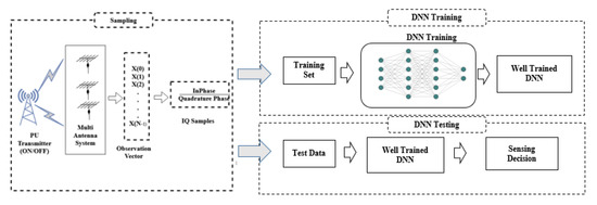
Figure 1. DNN Model.

Consider $X\left(n\right)={[x_1\left(n\right),x_2\left(n\right),\dots \dots x_M\left(n\right)]}^T$, where M represents the sample length of signal, $n=0,1,\dots \dots ,N-1$ denotes the $n^{th}$ received signal and $x_i\left(n\right)$ denotes the $n^{th}$ discrete time sample present at $i^{th}$ antenna of the CR terminal. The spectrum sensing problem can be formulated as a binary hypothesis testing problem [21]:

$$\begin{array}{c}\hfill H_1:X\left(n\right)=R\left(n\right)+U\left(n\right),\\ \hfill H_0:X\left(n\right)=U\left(n\right).\end{array}$$

(1)

Here, $R\left(n\right)$ denotes the signal vector that suffers from path loss and channel fading. $U\left(n\right)$ represents a circularly symmetric complex Gaussian (CSCG) noise vector with zero mean. Hence, hypothesis $H_1$ represents the presence of PU, while $H_0$ represents its absence.

Here, from the N received signals of the multi-antenna system, the in-phase (I) and quadrature (Q) components are extracted to obtain the modified set of received signals $\widehat{X}$ [21].

$$\begin{array}{c}\hfill X_I=Imag\left(X\left(n\right)\right)\\ \hfill X_Q=Real\left(X\left(n\right)\right)\\ \hfill \widehat{X}=(X_I,X_Q)\end{array}$$

(2)

Next, the received signals are labeled to obtain the train and test vectors. The labeled set is represented as follows:

$$(\widehat{X},Y)=({\widehat{x}}^{\left(1\right)},y^{\left(1\right)}),({\widehat{x}}^{\left(2\right)},y^{\left(2\right)}),\dots \dots \dots \dots \dots \dots ({\widehat{x}}^{\left(s\right)},y^{\left(s\right)})$$

(3)

where $\widehat{X}$ is the input to the deep neural network, with I-Q elements in our case. Y belongs to the set $\{1,0\}$ with labels $[1,0]$ and $[0,1]$ representing the hypothesis $H_1$ and $H_0$, respectively. s denotes the number of samples or observations, ${\widehat{x}}^{\left(s\right)}$ is the $s^{th}$ sample and $y^{\left(s\right)}$ is the label of the $s^{th}$ observation indicating the vacant or busy status. DNN is used to extract the features from the training set provided in a data driven manner. The test statistic is designed based on a binary classification problem in which the label is encoded as a one-hot vector:

$$Y=\left\{\begin{array}{cc}{[1,0]}^T,\hfill & H_1\hfill \\ {[0,1]}^T,\hfill & H_0\hfill \end{array}\right.$$

(4)

4. Proposed Methodology

Neural networks are a good tool for AI-based learning, so it is intended to be used here for spectrum sensing. A neural network-based DLSenseNet model uses a single node for simulation. This single node will receive the radio scene and analyze it at the local level. Spectrum sensing is classified as a binary classification problem of the received inputs and for that, the convolutional neural network is a better performer than other machine learning models. The DLSenseNet model is constructed by modifying the inception module. We added long short-term memory and fully connected layers to the inception module’s convolution layer. The LSTM layers were added for recognition of the temporal dependencies in the data, while the CNN layers investigate the spatial relations. Figure 2 illustrates the architecture of DLSenseNet.

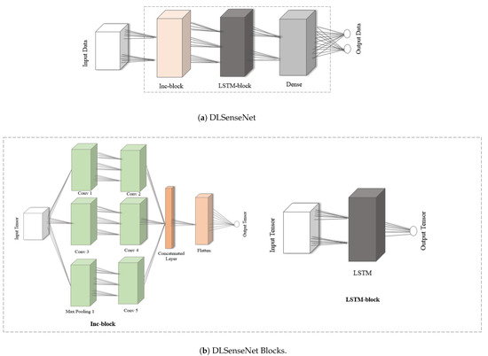
Figure 2. Network Architecture of DLSenseNet.

The input data in Figure 2a represents the in-phase and quadrature components of the received signal. The model consists of an Inc-block followed by an LSTM block and a dense layer generating spectrum occupancy output. A more detailed view of the model is shown in Figure 2b. The Inc-block consists of three parallel paths with different filter sizes. Two convolution layers and a max-pooling layer are present in the first hidden layer, which feed-forward to the next convolution layers. The addition of more layers is inspired by the inception model which balance generalization and complexity. For the proposed model, the optimized hyperparameters for the proposed DLSenseNet model are shown in Table 1.

Table 1. Model Hyperparameters.

Hyperparameter	DLSenseNet
Filters per convolution layer	64
Filters size	(1,1), (3,3) and (5,5)
Cells per LSTM layer	128
Neurons per FC layer	2,120,250,256,500
Optimizer	Adam
Initial learning rate	0.003
Batch size	64
Dropout ratio	0.2

The input to the system is the received signals from the multi-antenna system, which is then labeled for PU presence and absence. The expected output is correctly labeled on the basis of previously unseen observations. Since it is the in-phase and quadrature components that we are working on, the input vector is constituted by these two time domain details. Equation (5) depicts the input as $\widehat{X}$.

$$\begin{array}{c}\hfill X_I\leftarrow Imag\left(X\right),X_Q\leftarrow Real\left(X\right)\\ \hfill \widehat{X}\leftarrow (X_I,X_Q)\end{array}$$

(5)

Now, energy normalization was performed on this received complex signal, as represented in Equation (6), before splitting it into training and testing sets [22]. The M in Equation (6) represents the sample length of the signal. Normalization was also performed because models independent of energy have a better capacity of generalization even when the background noise changes. Also, without interference, the structure of the signals can be better exploited.

$$\begin{array}{c}\hfill Energy=\sum _{i=1}^M\left(\right|{\widehat{X}}_i{\left|\right)}^2\\ \hfill {\widehat{X}}_{norm}=\widehat{X}/Energy\end{array}$$

(6)

The DLSenseNet performs sensing for a CR node with ${\widehat{X}}_{norm}$ as the input. Equation (7) denotes the convolution operation with $C_i$ representing the output of $i^{th}$ convolution layer. Here, b is the bias, $w_{conv}$ is weight, and $\sigma$ is the activation function.

$$C_i=\sigma (b+\sum w_{conv}{\widehat{X}}_{norm})$$

(7)

Out of the three network connections from the input layer to the hidden layer, one is the max-pooling layer. Since the DLSenseNet architecture is inspired by the Inception architecture, the input is also passed through a max-pooling layer. The max-pooling layer utilizes the maximum value from neuron clusters in the previous layer. This also adjusts the effect of overfitting. In the Equation (8) that follows, the max-pooling operation is represented with pooling size of R.

$$p=ma{x}_{r\in R}\left({\widehat{X}}_{norm}\right)$$

(8)

The output features extracted by the convolution layers are then concatenated to be fed as input to the next layer. Equation (9) denotes the concatenation operation in which $C_2,C_4,C_5$ represent the outputs from the Conv 2, Conv 4, Conv 5 layers, respectively.

$$C_{concat}=Concatenate(C_2,C_4,C_5)$$

(9)

In a standard deep neural network, each layer’s signals can be transmitted only to the upper layer with the processing of samples independent of each other at different time intervals. Modeling of changes in sequences of time cannot be done, and encoding with only vectors of fixed dimensionality is possible. As such, the LSTM layer is added to the proposed network for determining the long term dependencies since IQ data belong to the time domain data characteristics. Furthermore, the signals modulated by different modulation schemes exhibit different characteristics, and LSTM is capable of learning these temporal dependencies effectively [23]. After concatenation, the dimensions of $C_{concat}$ were reshaped to be fed to the LSTM layer, which would learn the temporal features. The descriptive calculation of the LSTM layer outputs are denoted in Equation (10) which takes the present observation $C{\left(t\right)}_{concat}$ and past hidden layer output $h_{t-1}$ as input [24]. LSTM manages to learn long term dependencies by deciding upon information to be forgotten and remembered. After analysis of the current input and the previous state by $a_t$, the input gate $i_t$ decides upon which parts of $a_t$ are required to be added to the long term state $c_t$. The forget gate $f_t$ decides which parts should be erased and erases the unnecessary parts. Then, the output gate $o_t$ decides on the parts of $c_t$ to be shown as output. A short term state $h_t$ and a long term state $c_t$ exists in which memories are dropped and added by the gates. $w_{\ast }$ and $r_{\ast }$ (∗ represent $c,i,f,o$) are the weight matrices for the different gates, $\sigma$ denotes the sigmoid function, $\tanh$ denotes the hyperbolic tangent activation function and ⊙ represents the component-wise multiplication. The memory state $c_t$ and hidden state $h_t$ are forwarded as input to the next LSTM layer. The output from the LSTM layer to the fully connected layer is denoted as $L_t$.

$$\begin{array}{c}\hfill a_t=tanh(w_{c}C{\left(t\right)}_{concat}+r_c{h}_{t-1})\\ \hfill i_t=\sigma (w_{i}C{\left(t\right)}_{concat}+r_i{h}_{t-1})\\ \hfill f_t=\sigma (w_{f}C{\left(t\right)}_{concat}+r_f{h}_{t-1})\\ \hfill o_t=\sigma (w_{o}C{\left(t\right)}_{concat}+r_o{h}_{t-1})\\ \hfill c_t=i_t\odot a_t+f_t\odot c_{t-1}\\ \hfill h_t=o_t\odot \tanh \left(c_t\right)\end{array}$$

(10)

After the LSTM block processes the input, we have a fully connected dense layer that works upon the previous layer’s output, as stated in Equation (11). This layer then gives us the final output regarding the occupancy of the spectrum. The plots of spectrum occupancy are further elaborated in Section 6 of the results and discussion.

$$prob=\sigma (w_{dense}^T{L}_t+b)$$

(11)

The parameters and hyperparameters are initialized with random values which are to be tuned in the training process. The training split of observations is fed into the DLSenseNet which then calculates the label based on the initialized parameters. The categorical cross entropy, as shown in Equation (12), is the loss function which is used to minimize the error. ${\widehat{y}}^{ss}$ is the predicted output while y denotes the actual output. Based on this loss, the gradient is calculated, which is then used to update the weights, as denoted in Equation (13). In this way, the parameters are updated, which is then used to calculate the probabilities. Training is performed using the supervised learning mechanism and the parameters are updated accordingly.

$$Los{s}_{CCE}({\widehat{y}}^{ss},y)=-\sum _i(y\left[i\right]log{\widehat{y}}^{ss}\left[i\right]+(1-y\left[i\right])log\left({\widehat{y}}^{ss}\left[i\right]\right))$$

(12)

$$w^{ss}=w^{ss}-\eta {\left(t\right)}_{w^{ss}}Los{s}_{CCE}$$

(13)

Hence, the proposed network consists of five convolution layers, one max-pooling layer, one layer of LSTM, and a fully connected layer. The proposed deep neural network is trained for a different number of hidden layers and neurons. After extensive training, the layer size and number of cells are decided, which is denoted in Table 1. The ReLU and softmax functions are used as activation functions introducing non-linearity to the network. For the purpose of regularization, dropout is used. This is in order to prevent overfitting. The dropout ratio was kept at a value of 0.2. ADAM optimizer is utilized for optimization of the network parameters. The categorical cross entropy is the loss function that was used. The number of training epochs was 100, the tuning of which was done through early stopping with 6 epochs patience, which was applied for training the model to convergence. The learning rate was initialized at 0.003 and the batch size used for training was 64. The spectrum sensing works efficiently and in a robust manner. The DLSenseNet model was tested on a number of CNN and LSTM blocks to come up with the accurate results.

5. Experimental Setup

The design methodology is discussed here. Different models were used for classification and compared with our model in order to make our model more robust and accurate.

5.1. Dataset Generation and Preprocessing

The RadioML2016.10b [25] dataset is a publically available baseline dataset generated by O’Shea and Corgan [26]. The dataset consists of ten types of modulated signals with eight digital and two analog modulations. This includes SNR values and modulation type. The SNR values are distributed from −20 dB to +18 dB in 2 dB increments. Eight kinds of digitally modulated signals at different SNRs were used for our experiments. These signals are considered positive samples. The negative samples are the additive noise following the zero-mean circularly symmetric complex gaussian (CSCG) distribution generated with the same dimensions as the input signal. The training samples, consisting of $‘n’$ samples each, were fed into the deep neural network in $2\ast n$ vectors with the in-phase and quadrature components separated into complex time samples. Table 2 represents the dataset parameters. The dataset was partitioned into train, validation, and test sets.

Table 2. Dataset Parameters.

Parameters	Value
Modulation scheme	BPSK, QPSK, 8PSK, QAM16, QAM64, CPFSK, GFSK and PAM4
Sample length	64,128,256,512
SNR range	−20 dB∼18 dB in 2 dB increment
Training sample	153,000
Validation sample	51,000
Testing sample	51,000

5.2. Performance Evaluation Metrics

For performance evaluation, the model was trained and validated first before testing. The evaluation metrics considered here are the probability of detection ($P_d$), sensing error (SE) and probability of false alarm ($P_f$) [14]. $P_d$ is the probability of declaring the primary user’s presence when the primary user actually occupies the spectrum, and the $P_f$ is the probability of declaring that PU is present when the spectrum is actually vacant. Both the probabilities were calculated for different SNR values of the received signals. The performance metric SE was calculated by the averaged value of the probability of false alarm and the probability of miss detection ($P_m$). The probability of miss detection is the probability of declaring that the spectrum is vacant when actually the PU is present.

The performance metric values were calculated based on the confusion matrix, which is shown below.

		Predicted Diagnosis
		Signal	Noise
Actual Values	Signal	a	b
	Noise	c	d

Table 3 represents the formulas for calculating the performance evaluation metrics used for spectrum sensing. The confusion matrix values constructed after performing sensing on the test set were utilized for evaluating these values.

Table 3. Performance Evaluation Metrics.

Metric	Formulae
$P_d$	$\frac{a}{a+b}$
$P_m$	$1-P_d$
$P_f$	$\frac{c}{c+d}$
$SE$	$Average(P_f,P_m)$

6. Results and Discussion

The simulation results are presented here to demonstrate the proposed model’s performance. The effect of parameters such as modulation schemes, sample length and, classification models is investigated. This section presents and compares the results of our model with other deep neural network models, namely convolutional neural network (CNN), LeNet, residual network (ResNet), inception, LSTM, convolutional long short-term deep neural network (CLDNN) and previously reported spectrum sensing models of DetectNet [20] and CNN-LSTM [18]. For a desirable model, we need to achieve a low probability of false alarm, between 0 to 0.1 according to the IEEE 802.22 standard [27,28], low sensing error, and high probability of detection.

Figure 3 and Figure 4 represent the detection performance of all the neural network models with their false alarm for sample lengths of 64 and 128 on the signals modulated by QAM16 and QPSK modulation schemes for SNRs from −20 dB to 18 dB, respectively. It can be observed that the DLSenseNet model gives better detection performance in comparison to other models starting from low SNR values itself. The DLSenseNet and inception achieve better detection performance than other models. In addition, DLSenseNet attains $P_d$ value close to inception at −20 dB but outperforms inception by achieving lower $P_f$. For the varying sample lengths as well, the DLSenseNet proves its superior performance over other network models.

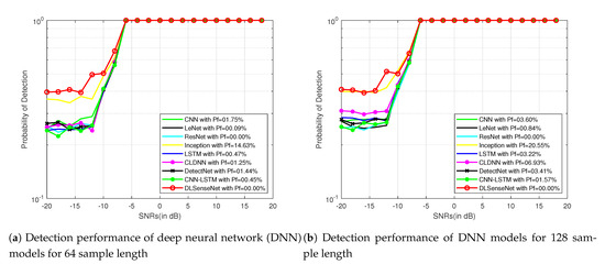
Figure 3. Detection performance of DNN models for QAM16 signals.

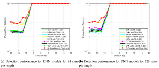
Figure 4. Detection performance of DNN models for QPSK signals.

Signals with lower SNRs (−20 dB to 0 dB) possess less information in comparison to higher SNRs (0 dB to 18 dB) because of being more distorted. Models with better recognition accuracy in lower SNRs perform better in the case of higher SNRs as well. To better display the the simulation results, Figure 5 and Figure 6 further represent the performance of all the models for 256 and 512 sample length signals modulated by QAM16 and QPSK for a varied range of the signal-to-noise ratio from −20 dB to 0 dB. The proposed model performs better than other solutions because it can understand the modulated structure of the signals. The network architecture of DLSenseNet consists of the component blocks of convolutional and LSTM layers. The CNN layers investigate the spatial relations, extracting useful information and learning the input data’s internal representations. LSTM layers help in the recognition of the temporal dependencies in the data to identify the short-term and long-term dependencies. The proposed DLSenseNet model efficiently combines the advantages of these two deep neural network architectures.

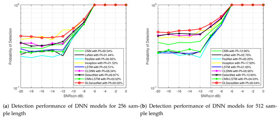
Figure 5. Detection performance of DNN models for QAM16 signals for −20 dB to 0 dB SNRs

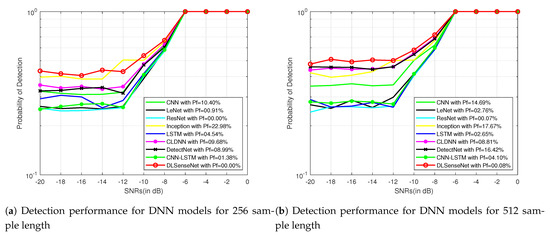
Figure 6. Detection performance of DNN models for QPSK signals for −20 dB to 0 dB SNRs.

The strength of versatility of the proposed model is proven by changing the characteristics of the PU signals. Figure 7 represents the detection performance of DLSenseNet over eight different modulation schemes with a sample length of 64 and SNRs range from −20 dB to 0 dB. As it can be observed, the detection performance difference between various modulated signals is relatively insignificant, implying the DLSenseNet performance is insensitive to the modulation order.

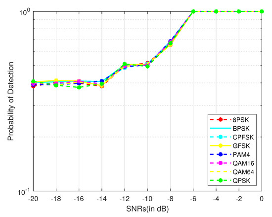
Figure 7. Impact of modulation schemes.

Figure 8 represents the trade-off between the detection probability and false alarm probability for all the network models over the QAM16 modulated signals with a sample length of 64. For demonstrating the proposed DLSenseNet model’s efficiency, the receiver operating characteristics (ROC) curves of the proposed model are compared with that of other models. It can be observed that the proposed model outperforms other models with an apparent margin. The CNN module of DLSenseNet scrutinizes the patterns of the received signal. The extracted features are provided as input to the LSTM such that the temporal features of the input sequence can be learned. The graphical features are processed by CNN, but it is not designed for processing temporal characteristics. The inception architecture inspires the proposed model since it is capable of balancing generalization and complexity. Additionally, the inception architecture performs similarly to the proposed model in terms of probability of detection but performs poorly in case of false alarm. The DLSenseNet model effectively combines the benefits of CNN, LSTM, and Inception, which is why it can outperform other models.

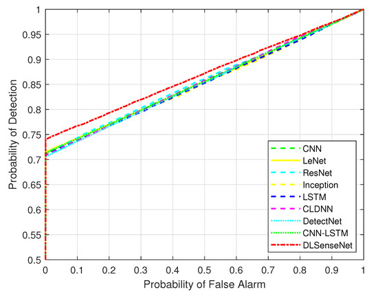
Figure 8. Receiver operating characteristics (ROC) Curves.

Table 4, Table 5, Table 6 and Table 7 represent the performance metrics for the 64, 128, 256 and 512 sample length signals modulated by QAM16 and QPSK. The different sample lengths are considered to represent the performance of the models for a wide range of sample lengths. The performance of the deep neural network models comprising of CNN and LSTM architectures is shown here for the detection performance in case of spectrum sensing, and the $P_d$ values are shown for an SNR value of −20 dB. $P_f$ of our DLSenseNet model is the lowest, which is desireable. The ResNet model is unable to achieve high $P_d$ despite having very low $P_f$. The $P_f$ of LeNet is also low; however, it cannot achieve high $P_d$ due to which its sensing error is high. The inception model also gives a good value of $P_d$ but the $P_f$ is much higher than other models. The sensing error of DLSenseNet is the lowest, proving a balance in the probability of detection and false alarm. As such, the DLSenseNet model achieves higher detection accuracy along with a low probability of false alarm. Therefore, the DLSenseNet model can detect the spectrum occupancy accurately.

Table 4. Comparison of performance metrics for 64 and 128 sample length QAM16 signals.

Models	64 Sample Length			128 Sample Length
	${\mathit{P}}_{\mathit{f}}$(%)	SE(%)	${\mathit{P}}_{\mathit{d}}$ (−20 dB) (%)	${\mathit{P}}_{\mathit{f}}$(%)	SE(%)	${\mathit{P}}_{\mathit{d}}$ (−20 dB) (%)
CNN	01.75	14.86	24.48	03.60	15.69	26.87
LeNet	00.09	14.51	24.96	00.84	14.63	27.17
ResNet	00.00	14.39	25.61	00.00	14.42	24.79
Inception	14.63	19.65	36.17	20.55	21.68	39.91
LSTM	00.47	14.75	24.13	03.22	15.35	28.48
CLDNN	01.25	14.87	25.15	06.93	17.36	31.08
DLSenseNet	00.00	12.99	39.60	00.00	12.93	40.97

Table 5. Comparison of performance metrics for 64 and 128 sample length QPSK signals.

Models	64 Sample Length			128 Sample Length
	${\mathit{P}}_{\mathit{f}}$ (%)	SE (%)	${\mathit{P}}_{\mathit{d}}$ (−20 dB) (%)	${\mathit{P}}_{\mathit{f}}$ (%)	SE (%)	${\mathit{P}}_{\mathit{d}}$ (−20 dB) (%)
CNN	01.59	14.91	27.14	04.98	16.09	27.37
LeNet	00.10	14.36	23.47	00.00	14.22	26.14
ResNet	00.00	14.60	23.58	00.00	14.58	25.55
Inception	16.98	20.43	35.93	20.32	21.75	39.39
LSTM	01.29	14.96	24.72	03.86	15.65	29.44
CLDNN	01.64	15.22	26.27	06.10	16.32	31.22
DLSenseNet	00.00	13.02	40.79	00.00	12.74	39.77

Table 6. Comparison of performance metrics for 256 and 512 sample length QAM16 signals.

Models	256 Sample Length			512 Sample Length
	${\mathit{P}}_{\mathit{f}}$ (%)	SE (%)	${\mathit{P}}_{\mathit{d}}$ (−20 dB) (%)	${\mathit{P}}_{\mathit{f}}$ (%)	SE (%)	${\mathit{P}}_{\mathit{d}}$ (−20 dB) (%)
CNN	09.54	17.88	30.69	12.96	19.04	35.31
LeNet	01.44	14.73	25.31	02.76	15.50	27.89
ResNet	00.00	14.53	23.97	00.20	14.55	25.77
Inception	21.53	22.03	38.48	17.93	18.68	39.71
LSTM	03.51	15.66	29.50	01.65	15.03	26.48
CLDNN	08.34	16.76	34.40	06.96	14.44	42.96
DLSenseNet	00.00	12.97	42.07	00.04	12.87	46.98

Table 7. Comparison of performance metrics for 256 and 512 sample length QPSK signals.

Models	256 Sample Length			512 Sample Length
	${\mathit{P}}_{\mathit{f}}$ (%)	SE (%)	${\mathit{P}}_{\mathit{d}}$ (−20 dB) (%)	${\mathit{P}}_{\mathit{f}}$ (%)	SE (%)	${\mathit{P}}_{\mathit{d}}$ (−20 dB) (%)
CNN	10.40	18.43	32.54	14.69	19.58	34.95
LeNet	00.91	14.67	26.26	02.76	15.51	26.87
ResNet	00.00	14.40	25.61	00.07	14.44	24.23
Inception	22.98	22.56	39.68	17.67	18.49	42.21
LSTM	04.54	15.85	29.24	02.65	15.34	28.94
CLDNN	09.68	17.45	35.50	08.81	15.03	43.87
DLSenseNet	00.00	13.09	43.32	00.08	12.76	47.70

Additionally, a comparison is shown among the sensing performance of the proposed DLSenseNet model and previously reported DetectNet [20] and CNN-LSTM [18] model in Table 8 and Table 9. The false alarm percentage and the probability of detection shown in Table 8 and Table 9 demonstrate that the DLSenseNet exhibits superiority over previous work. The proposed model lowers the false alarm and increases the probability of detection. The overall results indicate that the proposed model is a good choice for spectrum sensing in cognitive radio.

Table 8. Comparison of performance metrics to previous study for QAM16 signals.

Models	${\mathit{P}}_{\mathit{f}}$ (%)	SE (%)	${\mathit{P}}_{\mathit{d}}$ (−20 dB) (%)	${\mathit{P}}_{\mathit{f}}$ (%)	SE (%)	${\mathit{P}}_{\mathit{d}}$ (−20 dB) (%)
	64 Sample Length			128 Sample Length
Gao et al. [20]	01.44	14.89	26.37	03.41	15.74	27.72
Xie et al. [18]	00.45	14.88	24.10	01.57	14.96	25.28
DLSenseNet	00.00	12.99	39.60	00.00	12.93	40.97
	256 Sample Length			512 Sample Length
Gao et al. [20]	09.87	17.78	35.01	13.90	17.68	42.07
Xie et al. [18]	03.02	15.58	27.10	04.03	15.90	26.41
DLSenseNet	00.00	12.97	42.07	00.04	12.87	46.98

Table 9. Comparison of performance metrics to previous study for QPSK signals.

Models	${\mathit{P}}_{\mathit{f}}$ (%)	SE (%)	${\mathit{P}}_{\mathit{d}}$ (−20 dB) (%)	${\mathit{P}}_{\mathit{f}}$ (%)	SE (%)	${\mathit{P}}_{\mathit{d}}$ (−20 dB) (%)
	64 Sample Length			128 Sample Length
Gao et al. [20]	01.73	15.12	26.38	02.87	15.80	26.32
Xie et al. [18]	00.97	14.80	26.80	01.09	14.76	24.81
DLSenseNet	00.00	13.02	40.79	00.00	12.74	39.77
	256 Sample Length			512 Sample Length
Gao et al. [20]	08.99	17.45	32.68	16.42	18.70	45.90
Xie et al. [18]	01.38	14.83	25.23	04.10	15.94	28.01
DLSenseNet	00.00	13.09	43.32	00.08	12.76	47.70

The proposed work introduces the DLSenseNet mechanism for spectrum sensing. The models output whether the spectrum is occupied or vacant by considering the problem as a classification task. The better performance indicates accurate identification of primary user transmission over the spectrum.

7. Conclusions

Cognitive radio is a new Wireless Regional Area Network technology, which uses a spectrum opportunistically. Spectrum detection is a big issue in cognitive radio. Conventional spectrum sensing methods have inherent disadvantages to spectrum sensing for various reasons. A deep neural network based spectrum sensing model called “DLSenseNet” is proposed in this research. It shows an improvement compared to other sensing models, convolutional neural network, LSTM, CLDNN, residual network, inception, LeNet, and DetectNet. The performance of the models was tested with standard metrics of spectrum sensing. Our model demonstrates better performance in the same grade of services of the probability of detection and probability of false alarm.

References

- Gupta, A.; Jha, R.K. A Survey of 5G Network: Architecture and Emerging Technologies. IEEE Access 2015, 3, 1206–1232. [Google Scholar] [CrossRef]
- Cabric, D.; Mishra, S.M.; Brodersen, R.W. Implementation issues in spectrum sensing for cognitive radios. In Proceedings of the Conference Record of the Thirty-Eighth Asilomar Conference on Signals, Systems and Computers, Pacific Grove, CA, USA, 7–10 November 2004; Volume 1, pp. 772–776. [Google Scholar] [CrossRef]
- Marcus, M.J. Spectrum policy for radio spectrum access. Proc. IEEE 2012, 100, 1685–1691. [Google Scholar] [CrossRef]
- Mitola, J.; Maguire, G.Q. Cognitive radio: Making software radios more personal. IEEE Pers. Commun. 1999, 6, 13–18. [Google Scholar] [CrossRef]
- Haykin, S. Cognitive radio: Brain-empowered wireless communications. IEEE J. Sel. Areas Commun. 2005, 23, 201–220. [Google Scholar] [CrossRef]
- Lee, W.; Cho, D. Enhanced spectrum sensing scheme in cognitive radio systems with MIMO antennae. IEEE Trans. Veh. Technol. 2011, 60, 1072–1085. [Google Scholar] [CrossRef]
- Akyildiz, I.F.; Lo, B.F.; Balakrishnan, R. Cooperative spectrum sensing in cognitive radio networks: A survey. Phys. Commun. 2011, 4, 40–62. [Google Scholar] [CrossRef]
- Mishra, S.M.; Sahai, A.; Brodersen, R.W. Cooperative sensing among cognitive radios. In Proceedings of the IEEE International Conference on Communications, Istanbul, Turkey, 11–15 June 2006; Volume 4, pp. 1658–1663. [Google Scholar] [CrossRef]
- Goodfellow, I.; Bengio, Y.; Courville, A. Deep learning. arXiv 2017, arXiv:1312.6184v5. [Google Scholar]
- Peng, S.; Jiang, H.; Wang, H.; Alwageed, H.; Zhou, Y.; Sebdani, M.M.; Yao, Y.D. Modulation Classification Based on Signal Constellation Diagrams and Deep Learning. IEEE Trans. Neural Netw. Learn. Syst. 2019, 30, 718–727. [Google Scholar] [CrossRef] [PubMed]
- Lin, C.; Chang, Q.; Li, X. A deep learning approach for mimo-noma downlink signal detection. Sensors 2019, 19, 2526. [Google Scholar] [CrossRef] [PubMed]
- Vyas, M.R.; Patel, D.K.; López-Beńitez, M. Artificial neural network based hybrid spectrum sensing scheme for cognitive radio. In Proceedings of the IEEE International Symposium on Personal, Indoor and Mobile Radio Communications, PIMRC, Montreal, QC, Canada, 8–13 October 2017; pp. 1–7. [Google Scholar] [CrossRef]
- Han, D.; Sobabe, G.C.; Zhang, C.; Bai, X.; Wang, Z.; Liu, S.; Guo, B. Spectrum sensing for cognitive radio based on convolution neural network. In Proceedings of the 2017 10th International Congress on Image and Signal Processing, BioMedical Engineering and Informatics (CISP-BMEI), Shanghai, China, 14–16 October 2017; pp. 1–6. [Google Scholar] [CrossRef]
- Lee, W.; Kim, M.; Cho, D.H. Deep Cooperative Sensing: Cooperative Spectrum Sensing Based on Convolutional Neural Networks. IEEE Trans. Veh. Technol. 2019, 68, 3005–3009. [Google Scholar] [CrossRef]
- Chandhok, S.; Joshi, H.; Subramanyam, A.V.; Darak, S.J. Novel Deep Learning Framework for Wideband Spectrum Characterization at Sub-Nyquist Rate. arXiv 2019, arXiv:eess.SP/1912.05255. [Google Scholar]
- Zheng, S.; Chen, S.; Qi, P.; Zhou, H.; Yang, X. Spectrum sensing based on deep learning classification for cognitive radios. China Commun. 2020, 17, 138–148. [Google Scholar] [CrossRef]
- Peng, Q.; Gilman, A.; Vasconcelos, N.; Cosman, P.C.; Milstein, L.B. Robust Deep Sensing through Transfer Learning in Cognitive Radio. IEEE Wirel. Commun. Lett. 2020, 9, 38–41. [Google Scholar] [CrossRef]
- Xie, J.; Fang, J.; Liu, C.; Li, X. Deep Learning-Based Spectrum Sensing in Cognitive Radio: A CNN-LSTM Approach. IEEE Commun. Lett. 2020, 24, 2196–2200. [Google Scholar] [CrossRef]
- Cheng, Q.; Shi, Z.; Nguyen, D.N.; Dutkiewicz, E. Sensing OFDM Signal: A Deep Learning Approach. IEEE Trans. Commun. 2019, 67, 7785–7798. [Google Scholar] [CrossRef]
- Gao, J.; Yi, X.; Zhong, C.; Chen, X.; Zhang, Z. Deep Learning for Spectrum Sensing. IEEE Wirel. Commun. Lett. 2019, 8, 1727–1730. [Google Scholar] [CrossRef]
- Liu, C.; Wang, J.; Liu, X.; Liang, Y.C. Deep CM-CNN for Spectrum Sensing in Cognitive Radio. IEEE J. Sel. Areas Commun. 2019, 37, 2306–2321. [Google Scholar] [CrossRef]
- O’Shea, T.J.; West, N. Radio Machine Learning Dataset Generation with GNU Radio. In Proceedings of the GNU Radio Conference, Boulder, CO, USA, 12–16 September 2016. [Google Scholar]
- Rajendran, S.; Meert, W.; Giustiniano, D.; Lenders, V.; Pollin, S. Deep Learning Models for Wireless Signal Classification With Distributed Low-Cost Spectrum Sensors. IEEE Trans. Cogn. Commun. Netw. 2018, 4, 433–445. [Google Scholar] [CrossRef]
- Greff, K.; Srivastava, R.; Koutnik, J.; Steunebrink, B.; Schmidhuber, J. LSTM: A Search Space Odyssey. IEEE Trans. Neural Netw. Learn. Syst. 2017, 28, 2222–2232. [Google Scholar] [CrossRef] [PubMed]
- Liu, X.; Yang, D.; El Gamal, A. Deep neural network architectures for modulation classification. In Proceedings of the Conference Record of 51st Asilomar Conference on Signals, Systems and Computers, (ACSSC 2017), Pacific Grove, CA, USA, 29 October–1 November 2017; pp. 915–919. [Google Scholar] [CrossRef]
- O’Shea, T.J.; Corgan, J.; Clancy, T.C. Convolutional radio modulation recognition networks. In Engineering Applications of Neural Networks; Communications in Computer and Information Science; Springer: Cham, Switzerland, 2016; Volume 629, pp. 213–226. [Google Scholar] [CrossRef]
- P802.22/D6.0.0, May 2019—IEEE Draft Standard for Information Technology—Local and Metropolitan Area Networks—Specific Requirements—Part 22: Cognitive Radio Wireless Regional Area Networks (WRAN) Medium Access Control (MAC) and Physical Layer (PHY) Specifications: Policies and Procedures for Operation in the Bands that Allow Spectrum Sharing where the Communications Devices may Opportunistically Operate in the Spectrum of the Primary Service; IEEE: Piscataway, NJ, USA, 2019; pp. 1455–1465.
- Dehalwar, V.; Kalam, A.; Kolhe, M.L.; Zayegh, A. Compliance of IEEE 802.22 WRAN for field area network in smart grid. In Proceedings of the 2016 IEEE International Conference on Power System Technology, (POWERCON 2016), Wollongong, Australia, 28 September–1 October 2016. [Google Scholar] [CrossRef]
Publisher’s Note: MDPI stays neutral with regard to jurisdictional claims in published maps and institutional affiliations. |
© 2021 by the authors. Licensee MDPI, Basel, Switzerland. This article is an open access article distributed under the terms and conditions of the Creative Commons Attribution (CC BY) license (http://creativecommons.org/licenses/by/4.0/).