Computational Properties of General Indices on Random Networks

 and
and 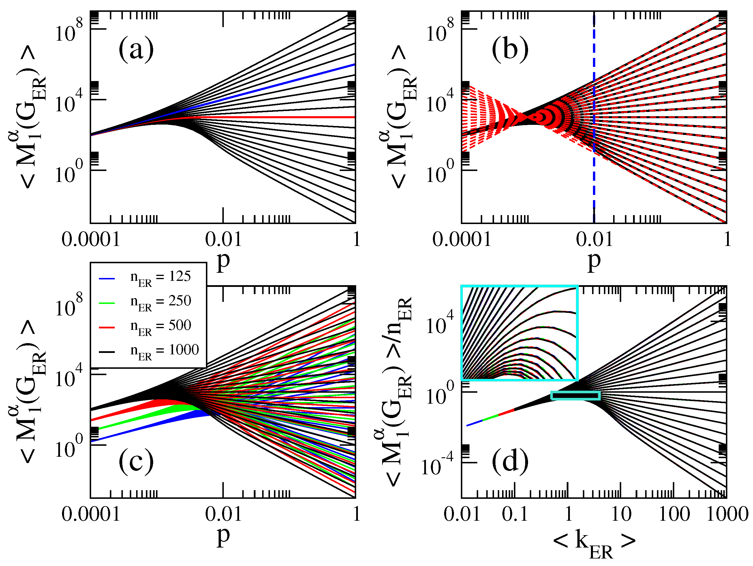
Abstract
1. Introduction
2. Erdös–Rényi Random Networks
2.1. Computational Properties of General Indices on Erdös–Rényi Random Networks
- (i)
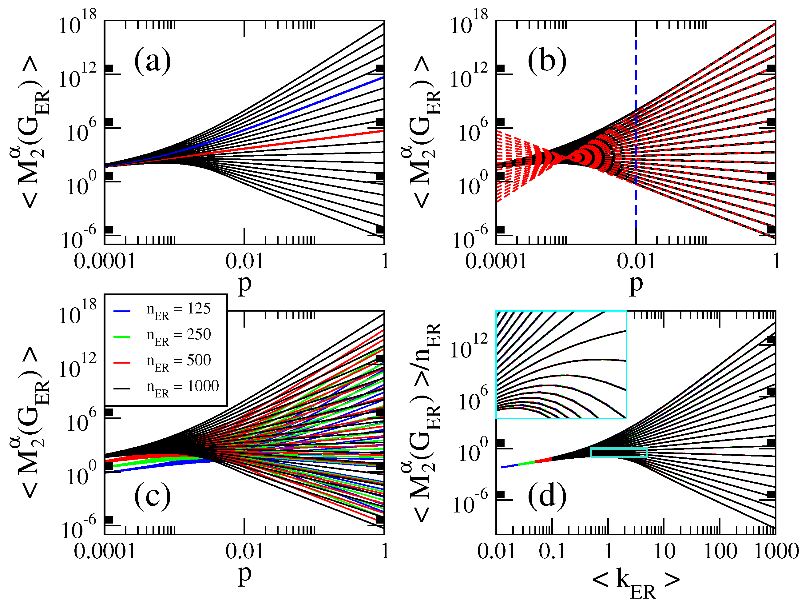
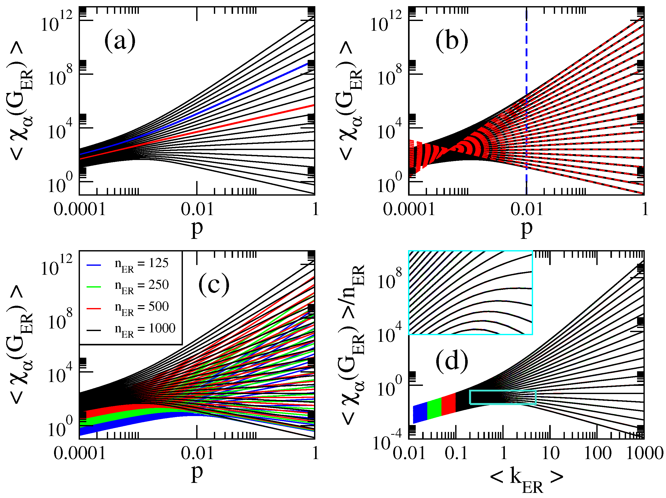
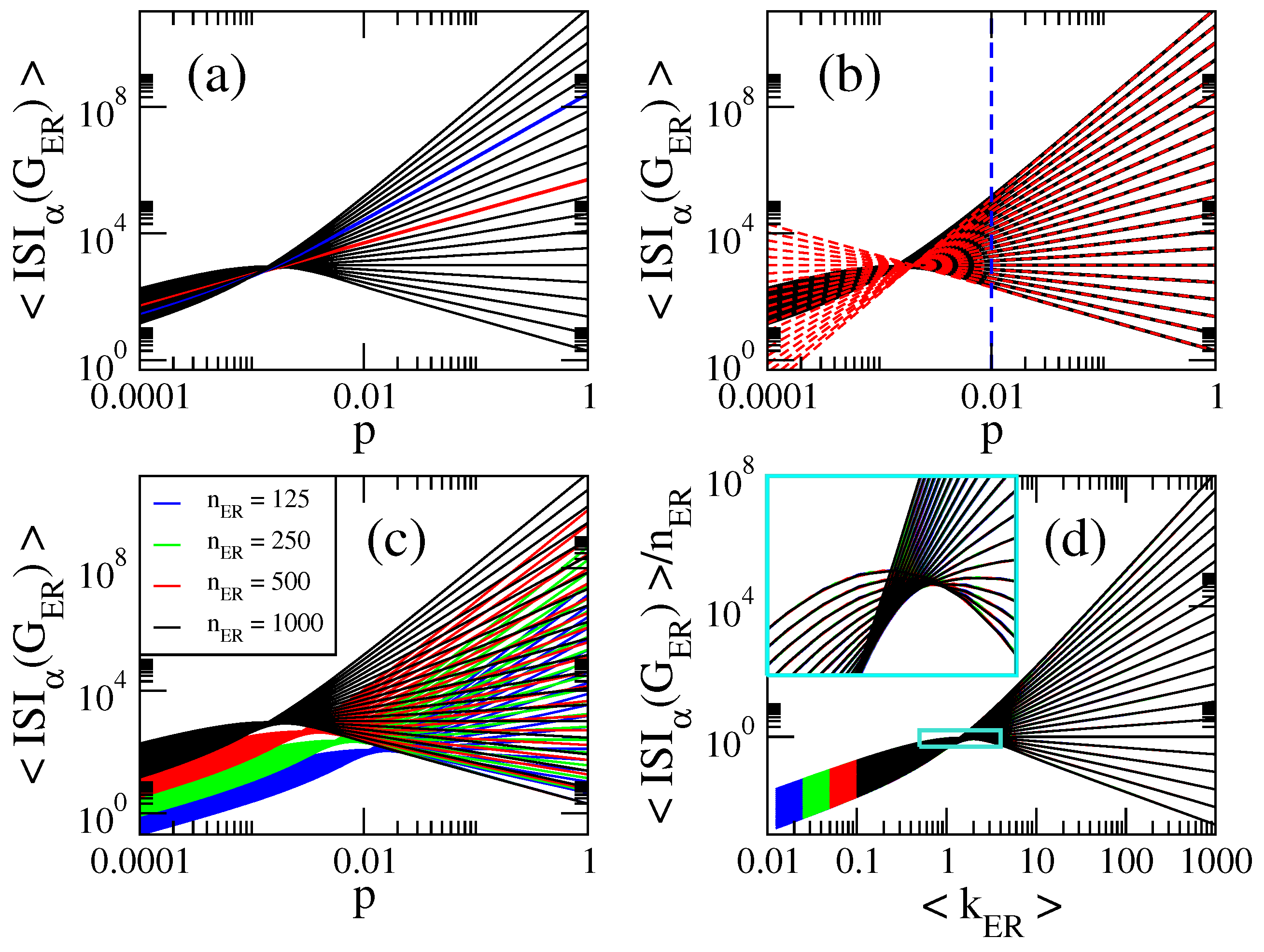
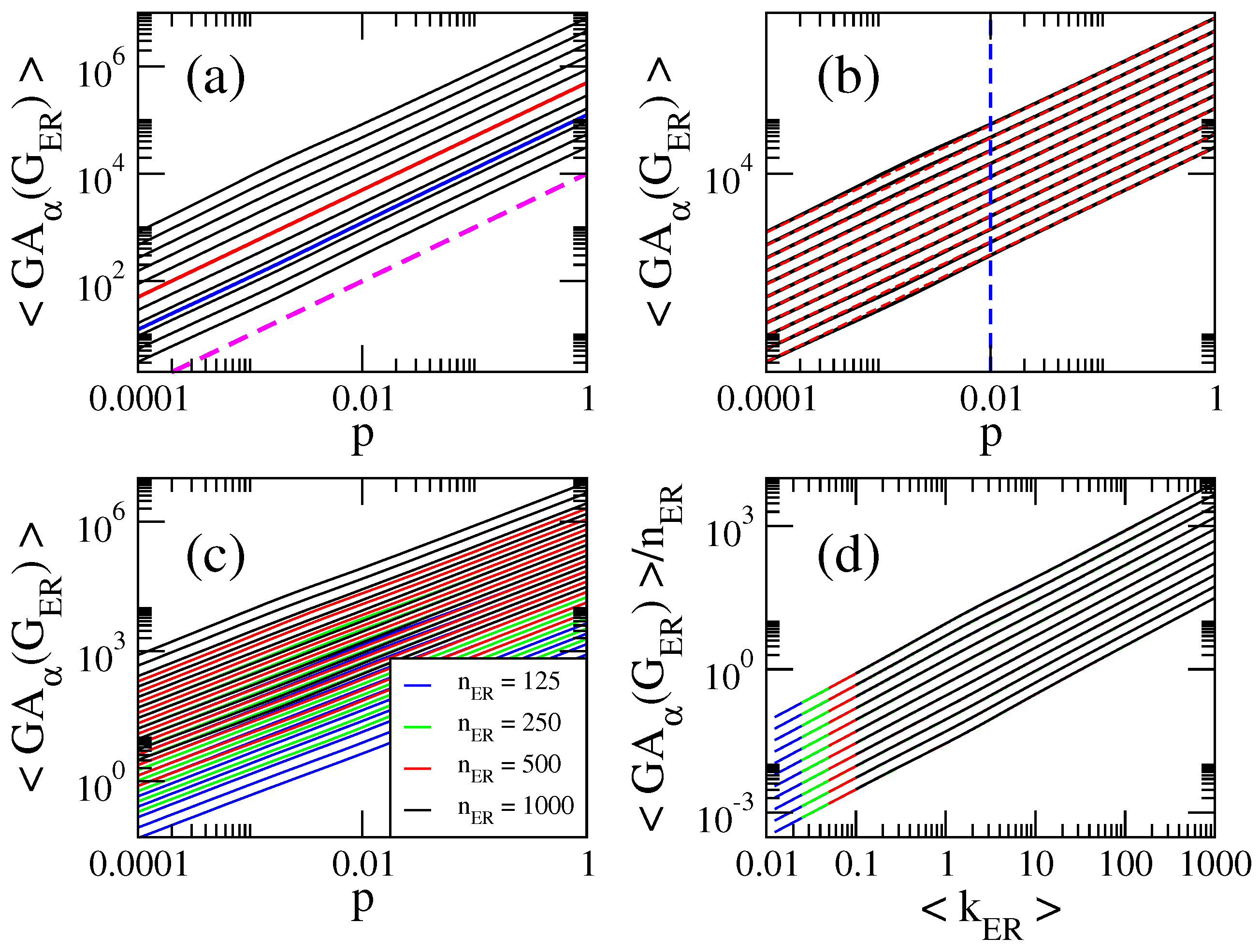
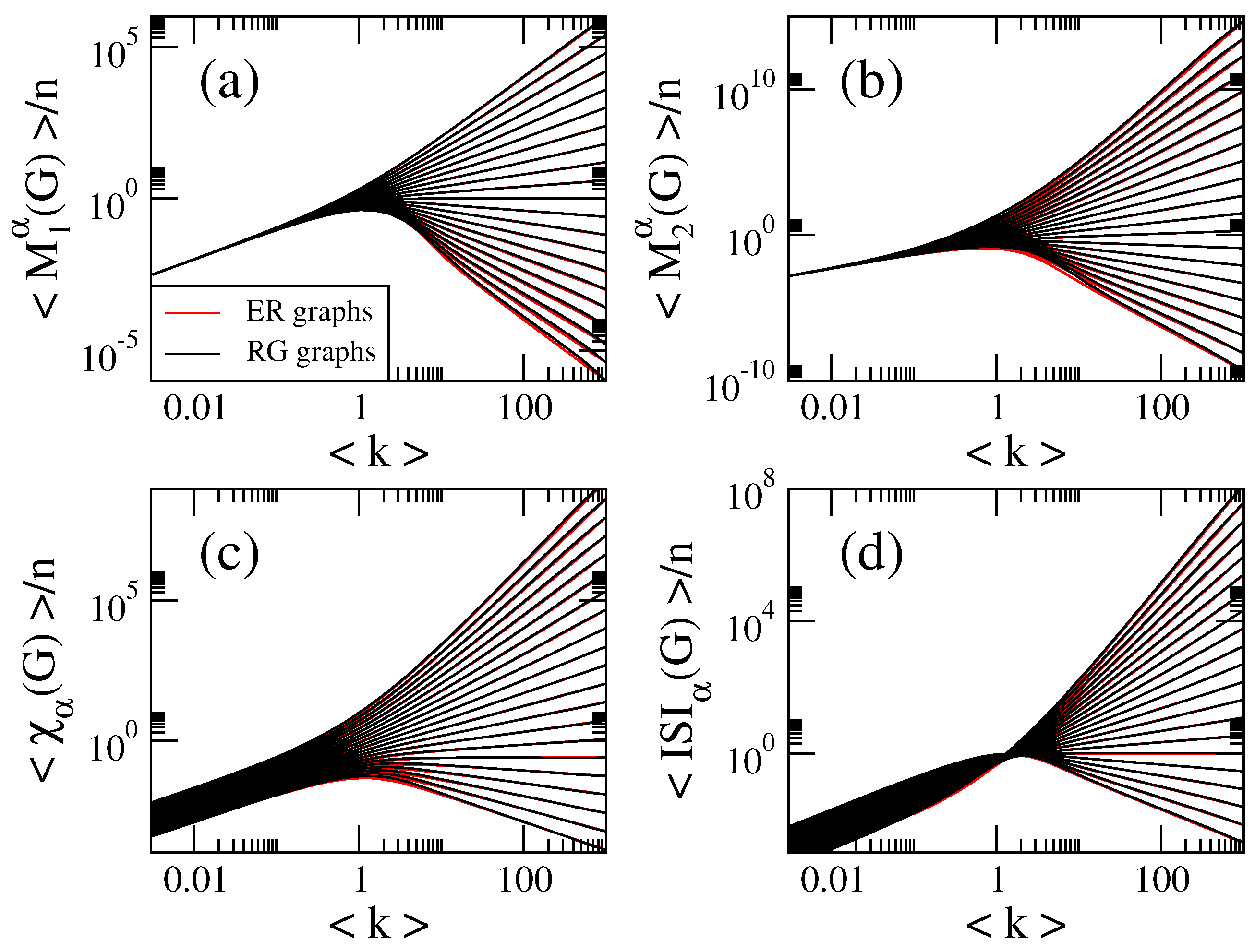
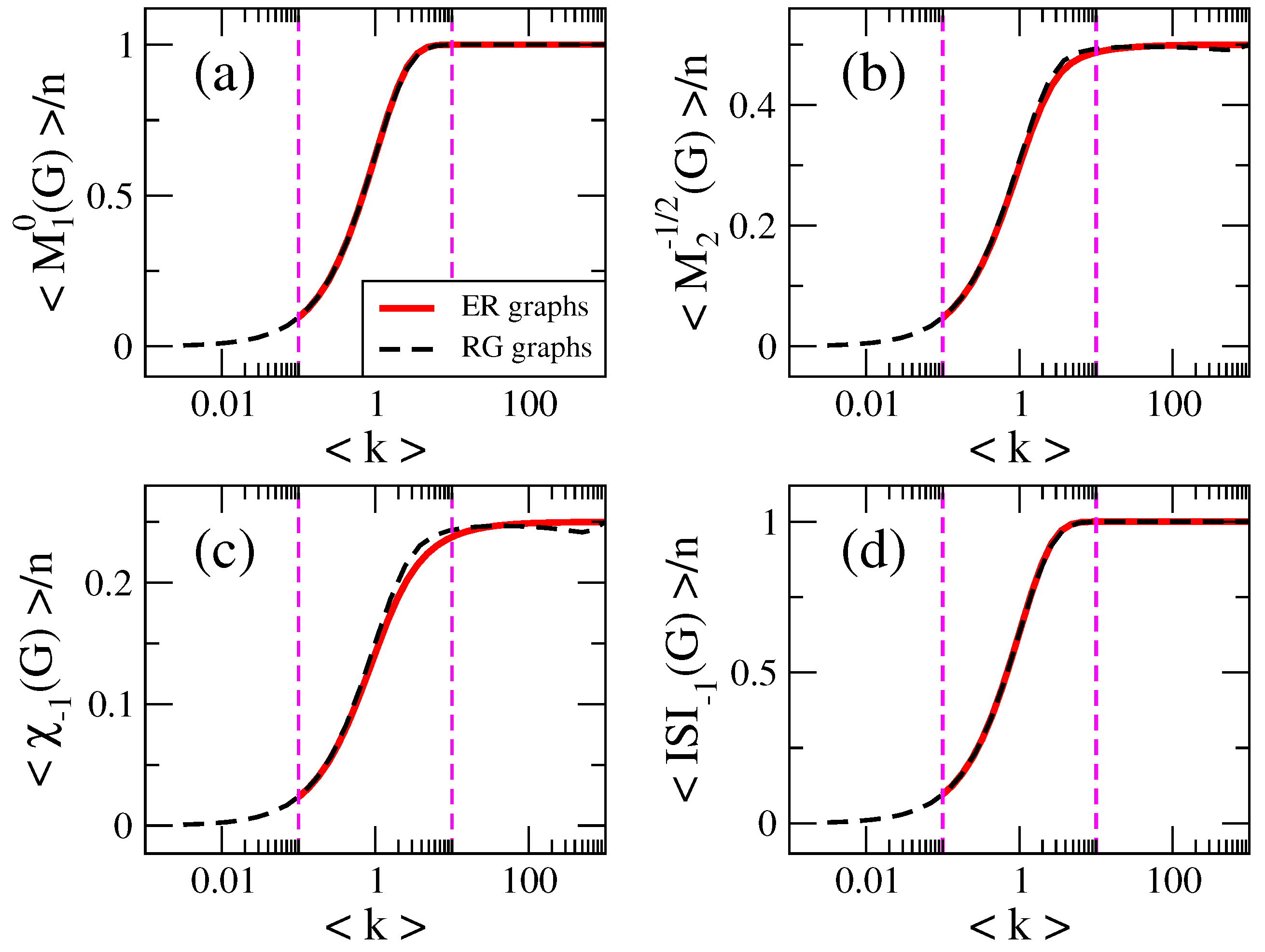
- The curves of , , and show three different behaviors as a function of p depending on the value of : for , they grow for small p, approach a maximum value and then decrease when p is further increased. For , they are monotonically increasing functions of p. For the curves saturate above a given value of p. See Figure 1a, Figure 2a, Figure 3a and Figure 4a.
- (ii)
- for , where is the average number of non-isolated vertices ; for , where is the average Randic index ; for , where is the average Harmonic index ; and for , so .
- (iii)
- All curves of grow linearly with p for all and ; see the magenta dashed line in Figure 5a, plotted to guide the eye.
- (iv)
- (v)
- Therefore, for , the average values of the indices we are computing here are well approximated by:
2.2. Scaling Properties of General Indices on Erdös–Rényi Random Networks
3. Random Geometric Graphs
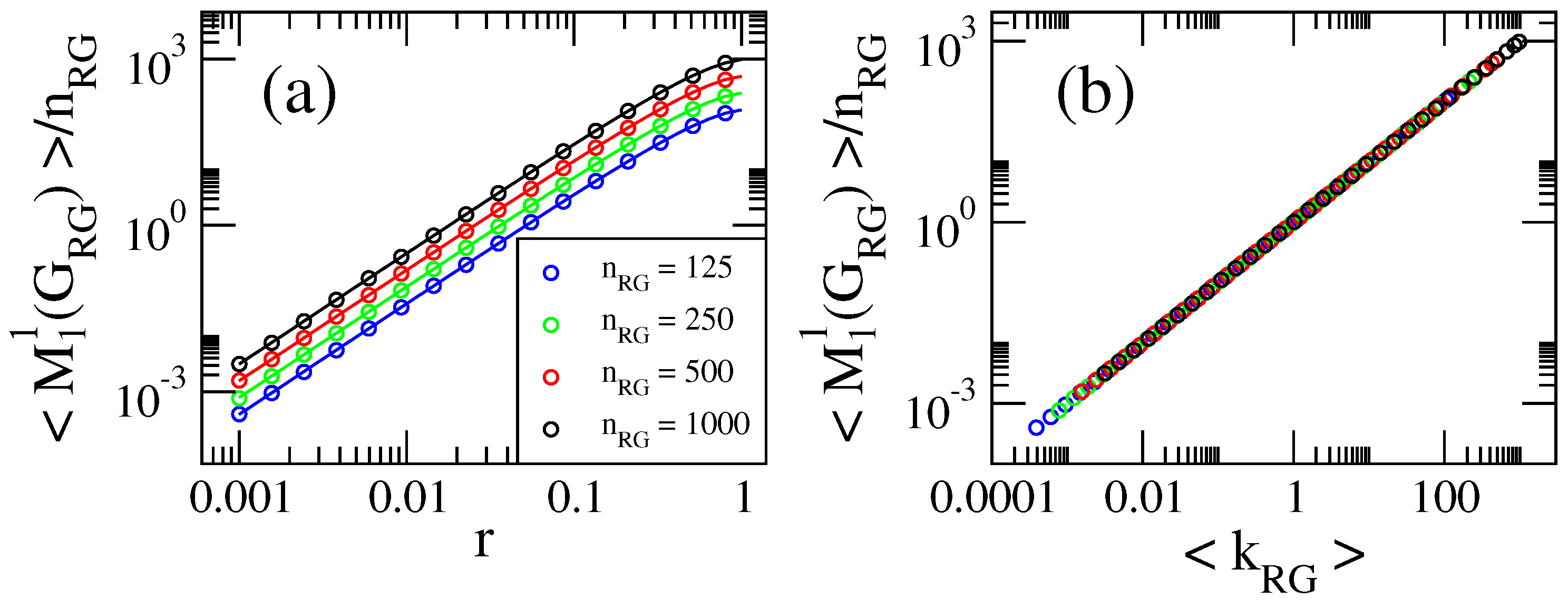
3.1. The Average Degree of Random Geometric Graphs
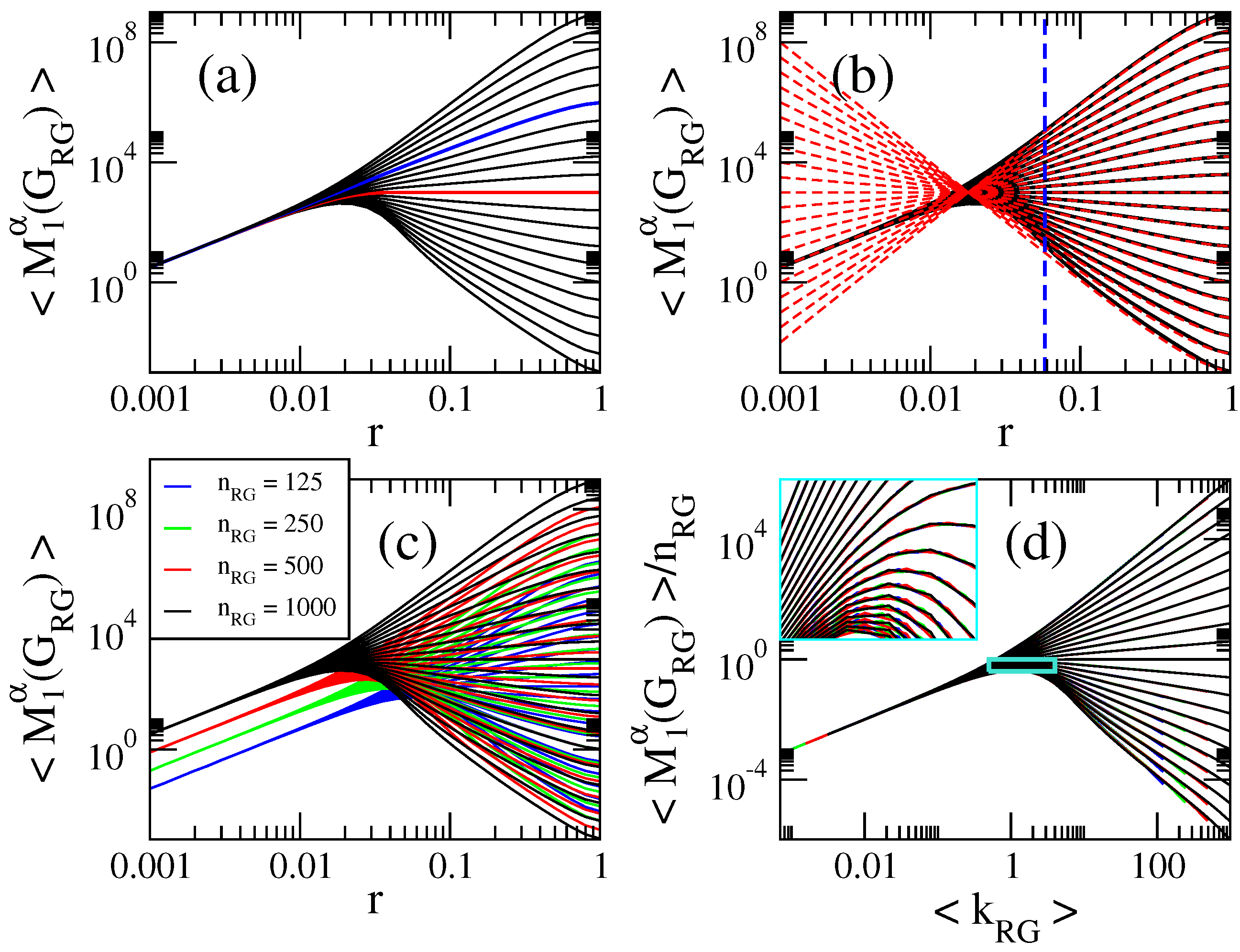
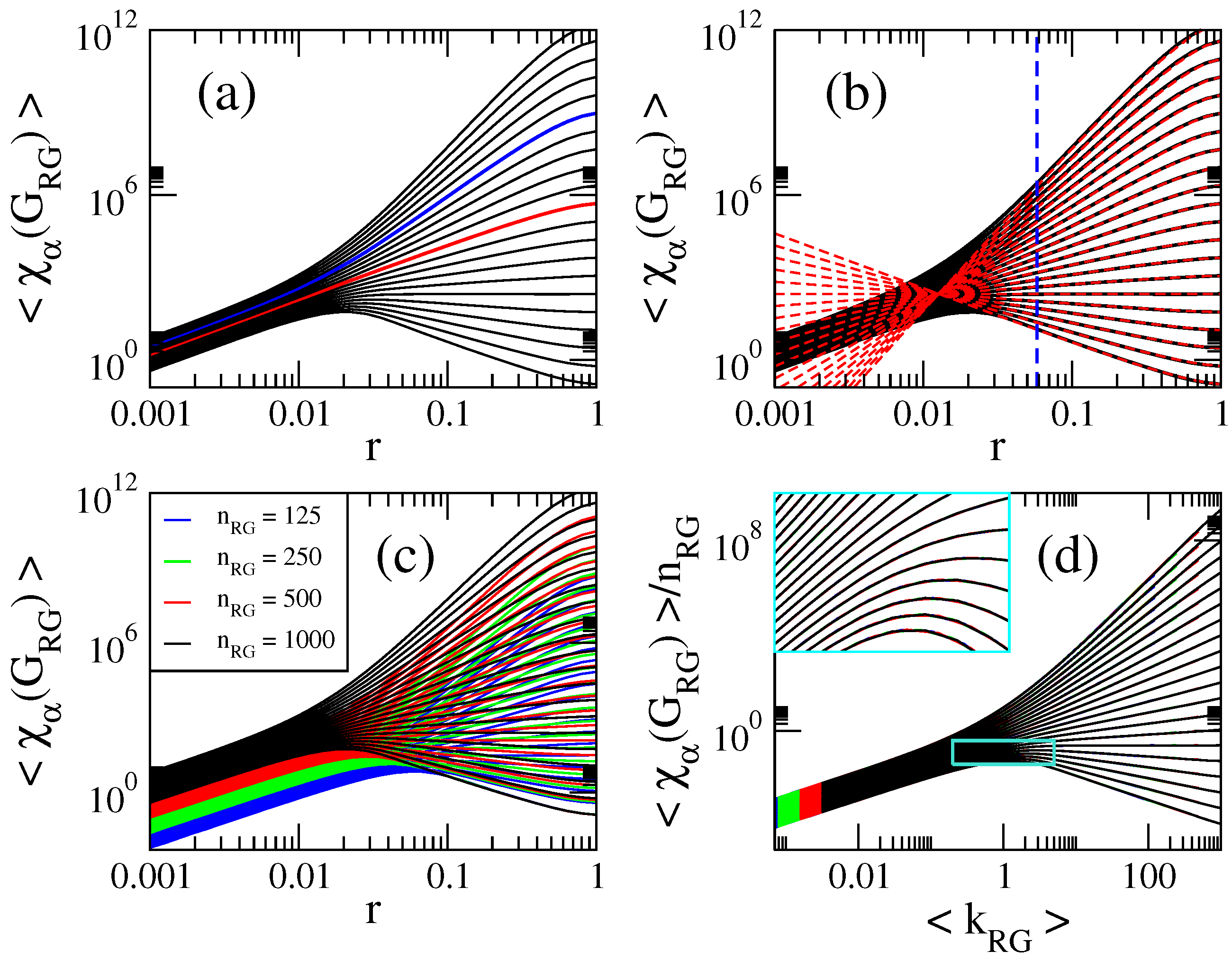
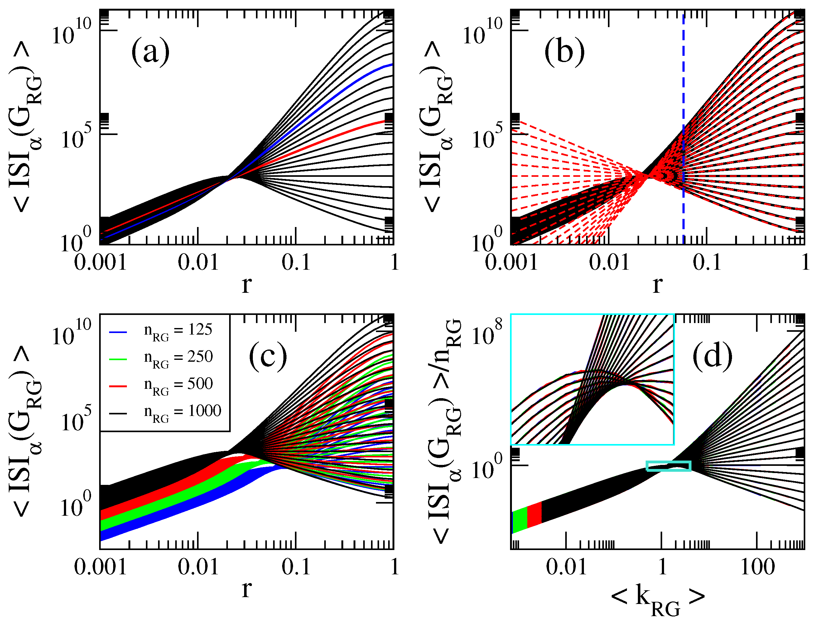
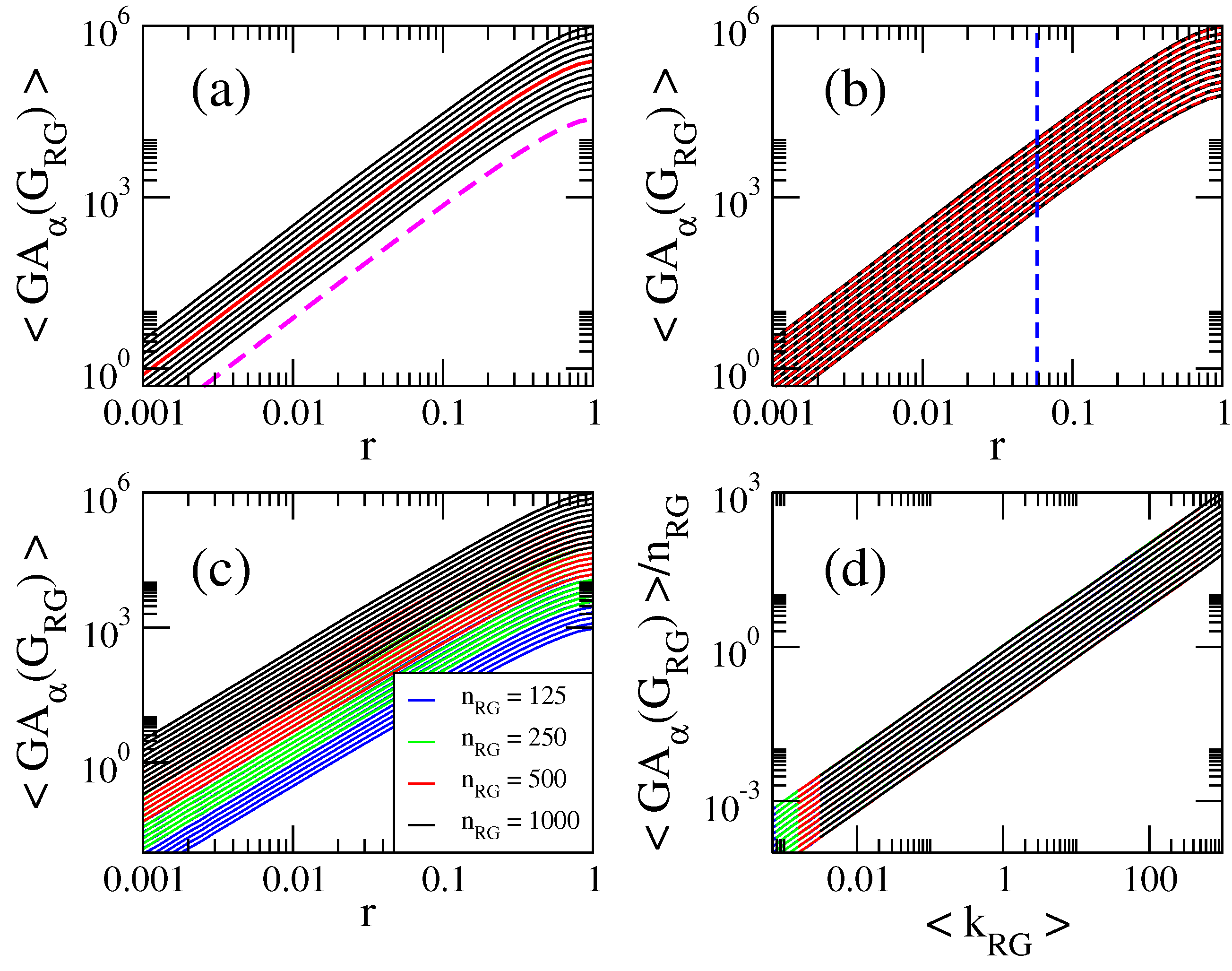
3.2. Computational Properties of General Indices on Random Geometric Graphs
3.3. Scaling Properties of General Indices on Random Geometric Graphs
4. Discussion and Conclusions
Author Contributions
Acknowledgments
Conflicts of Interest
References
- Wiener, H. Structural determination of paraffin boiling points. J. Am. Chem. Soc. 1947, 69, 17–20. [Google Scholar] [CrossRef] [PubMed]
- Hosoya, H. Topological index. A newly proposed quantity characterizing the topological nature of structural isomers of saturated hydrocarbons. Bull. Chem. Soc. Jpn. 1971, 44, 2331–2339. [Google Scholar] [CrossRef]
- Gutman, I.; Trinajstić, N. Graph theory and molecular orbitals. Total ϕ-electron energy of alternant hydrocarbons. Chem. Phys. Lett. 1972, 17, 535–538. [Google Scholar] [CrossRef]
- Nikolic, S.; Kovacevic, G.; Milicevic, A.; Trinajstic, N. The Zagreb indices 30 years after. Croat. Chem. Acta 2003, 76, 113–124. [Google Scholar]
- Randić, M. On characterization of molecular branching. J. Am. Chem. Soc. 1975, 97, 6609–6615. [Google Scholar] [CrossRef]
- Randić, M. Novel graph theoretical approach to heteroatoms in quantitative structure-activity relationships. Chemom. Int. Lab. Syst. 1991, 10, 213–227. [Google Scholar] [CrossRef]
- Randić, M. On computation of optimal parameters for multivariate analysis of structure-property relationship. J. Comput. Chem. 1991, 12, 970–980. [Google Scholar] [CrossRef]
- Miličević, A.; Nikolić, S. On variable Zagreb indices. Croat. Chem. Acta 2004, 77, 97–101. [Google Scholar]
- Li, X.; Zheng, J. A unified approach to the extremal trees for different indices. MATCH Commun. Math. Comput. Chem. 2005, 54, 195–208. [Google Scholar]
- Li, X.; Zhao, H. Trees with the first smallest and largest generalized topological indices. MATCH Commun. Math. Comput. Chem. 2004, 50, 57–62. [Google Scholar]
- Nikolić, S.; Miličević, A.; Trinajstić, N.; Jurić, A. On use of the variable Zagreb Index in QSPR: Boiling points of Benzenoid hydrocarbons. Molecules 2004, 9, 1208–1221. [Google Scholar] [CrossRef] [PubMed]
- Zhou, B.; Trinajstić, N. On general sum-connectivity index. J. Math. Chem. 2010, 47, 210–218. [Google Scholar] [CrossRef]
- Rodríguez, J.M.; Sigarreta, J.M. New results on the Harmonic index and its generalizations. MATCH Commun. Math. Comput. Chem. 2017, 78, 387–404. [Google Scholar]
- Hafeez, S.; Farooq, R. On generalized inverse sum indeg index and energy of graphs. AIMS Math. 2020, 5, 2388–2411. [Google Scholar] [CrossRef]
- Das, K.C.; Gutman, I.; Furtula, B. Survey on geometric–arithmetic indices of graphs. MATCH Commun. Math. Comput. Chem. 2011, 65, 595–644. [Google Scholar]
- Wilczek, P. New geometric–arithmetic indices. MATCH Commun. Math. Comput. Chem. 2018, 79, 5–54. [Google Scholar]
- Aouchiche, M.; Ganesan, V. Adjusting geometric–arithmetic index to estimate boiling point. MATCH Commun. Math. Comput. Chem. 2020, 84, 483–497. [Google Scholar]
- Solomonoff, R.; Rapoport, A. Connectivity of random nets. Bull. Math. Biophys. 1951, 13, 107–117. [Google Scholar] [CrossRef]
- Erdös, P.; Rényi, A. On random graphs. Publ. Math. 1959, 6, 290–297. [Google Scholar]
- Erdös, P.; Rényi, A. On the evolution of random graphs. Inst. Hung. Acad. Sci. 1960, 5, 17–61. [Google Scholar]
- Erdös, P.; Rényi, A. On the strength of connectedness of a random graph. Acta Math. Hung. 1961, 12, 261–267. [Google Scholar] [CrossRef]
- Dall, J.; Christensen, M. Random geometric graphs. Phys. Rev. E 2002, 66, 016121. [Google Scholar] [CrossRef] [PubMed]
- Penrose, M. Random Geometric Graphs; Oxford University Press: Oxford, UK, 2003. [Google Scholar]
- Martínez-Martínez, C.T.; Méndez-Bermúdez, J.A.; Rodríguez, J.M.; Sigarreta, J.M. Computational and analytical studies of the Randić index in Erdös–Rényi models. Appl. Math. Comput. 2020, 377, 125137. [Google Scholar]
- Martínez-Martínez, C.T.; Méndez-Bermúdez, J.A.; Rodríguez, J.M.; Sigarreta, J.M. Computational and analytical studies of the harmonic index in Erdös–Rényi models. MATCH Commun. Math. Comput. Chem. 2021, 85. in press. [Google Scholar]
- Estrada, E.; Sheerin, M. Random rectangular graphs. Phys. Rev. E 2015, 91, 042805. [Google Scholar] [CrossRef]
- Metha, M.L. Random Matrices; Elsevier: Amsterdam, The Netherlands, 2004. [Google Scholar]
- Haake, F. Quantum Signatures of Chaos; Springer: Berlin, Germany, 2010. [Google Scholar]
- Mendez-Bermudez, J.A.; Alcazar-Lopez, A.; Martinez-Mendoza, A.J.; Rodrigues, F.A.; Peron, T.K.D.M. Universality in the spectral and eigenfunction properties of random networks. Phys. Rev. E 2015, 91, 032122. [Google Scholar] [CrossRef]
- Alonso, L.; Mendez-Bermudez, J.A.; Gonzalez-Melendrez, A.; Moreno, Y. Weighted random-geometric and random-rectangular graphs: Spectral and eigenfunction properties of the adjacency matrix. J. Complex Netw. 2018, 6, 753. [Google Scholar] [CrossRef]
- Torres-Vargas, G.; Fossion, R.; Mendez-Bermudez, J.A. Normal mode analysis of spectra of random networks. Physica A 2020, 545, 123298. [Google Scholar] [CrossRef]
- Aguilar-Sanchez, R.; Mendez-Bermudez, J.A.; Rodrigues, F.A.; Sigarreta-Almira, J.M. Topological versus spectral properties of random geometric graphs. arXiv 2020, arXiv:2007.02453. [Google Scholar]


© 2020 by the authors. Licensee MDPI, Basel, Switzerland. This article is an open access article distributed under the terms and conditions of the Creative Commons Attribution (CC BY) license (http://creativecommons.org/licenses/by/4.0/).
Share and Cite
Aguilar-Sánchez, R.; Herrera-González, I.F.; Méndez-Bermúdez, J.A.; Sigarreta, J.M. Computational Properties of General Indices on Random Networks. Symmetry 2020, 12, 1341. https://doi.org/10.3390/sym12081341
Aguilar-Sánchez R, Herrera-González IF, Méndez-Bermúdez JA, Sigarreta JM. Computational Properties of General Indices on Random Networks. Symmetry. 2020; 12(8):1341. https://doi.org/10.3390/sym12081341
Chicago/Turabian StyleAguilar-Sánchez, R., I. F. Herrera-González, J. A. Méndez-Bermúdez, and José M. Sigarreta. 2020. "Computational Properties of General Indices on Random Networks" Symmetry 12, no. 8: 1341. https://doi.org/10.3390/sym12081341
APA StyleAguilar-Sánchez, R., Herrera-González, I. F., Méndez-Bermúdez, J. A., & Sigarreta, J. M. (2020). Computational Properties of General Indices on Random Networks. Symmetry, 12(8), 1341. https://doi.org/10.3390/sym12081341