Formation of the Dynamic Energy Cascades in Quartic and Quintic Generalized KdV Equations

Abstract

In this study we investigate for the first time the formation of dynamical energy cascades in higher order KdV-type equations. In the beginning we recall what is known about the dynamic cascades for the classical KdV (quadratic) and mKdV (cubic) equations. Then, we investigate further the mKdV case by considering a richer set of initial perturbations in order to check the validity and persistence of various facts previously established for the narrow-banded perturbations. Afterwards we focus on higher order nonlinearities (quartic and quintic) which are found to be quite different in many respects from the mKdV equation. Throughout this study we consider both the direct and double energy cascades. It was found that the dynamic cascade is always formed, but its formation is not necessarily accompanied by the nonlinear stage of the modulational instability. The direct cascade structure remains invariant regardless of the size of the spectral domain. In contrast, the double cascade shape can depend on the size of the spectral domain, even if the total number of cascading modes remains invariant. The results obtained in this study can be potentially applied to plasmas, free surface and internal wave hydrodynamics.

1. Introduction

When we want to describe an open or a closed physical system, the main question is to describe the energy flux inside this system and with surrounding environment. The energy transport along the wavenumbers in Fourier space is generally called the energy cascade. An elegant idea to describe this cascade in turbulent flows was first proposed by Richardson in 1922 [1]. His empirical description was put by the author in the form of a verse:

• Big whirls have little whirls;
• Which feed on their velocity;
• And little whirls have lesser whirls;
• And so on to viscosity.

In this poetic way Richardson described the energy transport among turbulent vortexes over the scales which ends by the dissipative region. This semi-empirical argument was made more accurate by Kolmogorov in his famous 1941 paper (whose English translation can be found in [2]) where he proposed the universal energy spectrum $\sim {\ell }^{5/3}$ for the strong homogeneous isotropic turbulence (here ℓ is characteristic size of a vortex). A similar approach applied to weakly nonlinear wave systems resulted in the development of the so-called Weak (or Wave) Turbulence Theory (WTT) [3] where the spectrum is not universal anymore and it depends on the dispersion function. However, the spectrum shape still remains a power law as in the strong turbulence theory. In terms of the nonlinearity parameter $\epsilon$ the strong turbulence theory corresponds to ${\epsilon }_{ST}\sim \mathcal{O}\left(1\right)$ while the WTT is situated in the range ${\epsilon }_W\sim \mathcal{O}\left({10}^{-2}\right)$. Physically relevant definition of the parameter of nonlinearity is of paramount importance in the WTT and depends on the essential characteristics of the system under study. It can be the ratio of the particle velocity to the phase velocity as in the case of oceanic planetary motion (the so-called barotropic vorticity equation) or the ratio of the wave amplitude to the wave length (the so-called steepness) for surface water waves (NLS), or the ratio of the wave amplitude to the finite characteristic fluid layer depth in shallow waters (KdV).

The model of the dynamic energy cascade for the case of intermediate (moderate) nonlinearities ${\epsilon }_M\sim \mathcal{O}\left({10}^{-1}\right)$ was proposed quite recently in 2012 [4] and studied analytically in [5,6]. Since the dynamic energy cascade model is based on the Modulational Instability (MI) mechanism, the first developments were made the the case of the Nonlinear Schrödinger (NLS) equation and its modifications. The spectrum shape is deduced from the Incremental Chain Equations (ICE) which strongly relies on the knowledge of the instability interval. Fortunately this information is readily available for NLS-type equations in the literature.

On the other hand, the MI can be encountered in other types of model equations. It is important to study the dynamic energy cascade formation in these models as well. The present article is entirely devoted to some generalized Korteweg–de Vries (KdV)-type equations. The celebrated original KdV equation was derived for the first time for surface waves in shallow waters [7,8] in order to explain the phenomenon of solitary waves:

$$\mathrm{KdV}\left(u\right)\doteq u_t+u_{xxx}+\beta u{u}_x=0,$$

(1)

where the first term is responsible for the time evolution, the second term is the dispersion and the third one is the advective nonlinearity. However, it is known that the classical KdV Equation (1) does not possess the MI. Later some extended versions of the KdV equation were derived for both surface [9] and internal [10] waves. By making appropriate changes of variables, it can be reduced to the following modified (m)KdV equation:

$$\mathrm{mKdV}\left(u\right)\doteq u_t+u_{xxx}+\beta u^2{u}_x=0.$$

(2)

It is known that Equation (2) is integrable and it possesses the MI for $\beta >0$. For negative values of parameter $\beta <0$ its behaviour is similar to the KdV in the respect of the MI. As integrability for equations of KdV-type requires the existence of higher infinitesimal symmetries and/or higher conservation laws [11], it yields neither explicit nor constructive information about the form of a solution corresponding to the specific initial excitation. On the other hand, modulation instability describes conditions when periodic travelling waves are stable/unstable in the frame of an evolutionary dispersive PDE. Accordingly, a priori this is not at all clear how to gain any information from the integrability of a KdV-type equation for studying modulation instability. For the particular cases $p=1$ and $p=2$, solutions can be written out in terms of elliptic functions and elliptic integrals of modulus depending of the parameters of the initial PDE. These analytical solutions also do not suit for studying modulation instability, instead a small parameter is usually introduced and a perturbation technique is used which allows construction of an explicit form of the approximate solution, see, e.g., [12]. This technique can be used both for integrable and non-integrable equations.

Formally all these model equations can be encompassed into a single gKdV framework:

$$\mathrm{gKdV}\left(u\right)\doteq u_t+u_{xxx}+(\alpha u+\beta u^2+\delta u^3+\gamma u^4)u_x=0,$$

(3)

which generates the KdV, mKdV, quartic and quintic gKdV equations for particular choices of coefficients $\alpha$, $\beta$, $\delta$ and $\gamma$. Quartic and quintic gKdV equations will be studied extensively numerically below.

In general, there are only few known mathematical facts about higher order KdV-type models. The global well-posedness of the quartic gKdV equation in some critical spaces was shown in [13], while the stability of periodic travelling waves in the gKdV equation was studied in [14,15]. A general classification of the equations of KdV-type according to their (inexplicit) integrability properties can be found in [11].

As we already mentioned above, the shape of the energy spectrum was computed in the NLS-type equations based on the explicit knowledge of the instability interval with finite measure. In the case of the KdV-type equations and nonlinearity of order nonlinearities $\mathcal{O}\left({10}^{-1}\right)$ such finite intervals do not exist, since any mode with the wave number $k_0>0$ is modulationally unstable (if the equation has the MI, of course). This fact prevents the direct transposition of NLS predictions to the family of KdV-type equations. Nevertheless, we decided to study the dynamic energy cascades in several KdV-type models numerically.

In general, the MI is an effect which describes a special type of the instability of a single spectral component subject to narrow band excitation in an experiment (regardless whether it is numerical or laboratory). In our previous investigations [16,17] we followed this ideology and all the numerical experiments toward the observation of the direct and inverse cascades had only two spectral harmonics in the initial condition (i.e., the base wave $k_0$ along with its modulation $K_0\ll k_0$).

On the other hand, in real-world laboratory experiments it is extremely difficult to excite precisely only two spectral harmonics. It is always a finite range which appears. Consequently, it is interesting to study this situation in numerical experiments as well in order to determine the limits of the survivability of the dynamical energy cascade [6,18]. Additional motivation comes from the fact that the so-called Benjamin–Feir Index (BFI) [19], which characterizes the likelihood of freak wave formation in an open ocean, is also based on the effect of the MI in the presence of a fairly broad spectrum. There is a direct connection between the BFI and the increment chain equations which describe the cascade formation [20]. It should be noted that the BFI was introduced, strictly speaking, for surface waves in deep water which are described by the NLS-type equations. However, this notion might be transposed to the mKdV case as well, since the analytical bridges between NLS and (m)KdV are well studied [21] (and the references therein).

Even if historically the KdV equation (and related models) was proposed first as a model equation for surface waves [22,23,24], later it found applications in many other fields such as plasma physics [25,26,27], acoustic and internal waves in the ocean [28,29,30]. That is why the study of this equation along with its various modifications is important. The big advantage of the classical KdV (1) and mKdV (2) equations consists in their exceptional mathematical properties—i.e., the integrability, which allows a deep mathematical study. However, even in this case it does not allow to describe exactly the properties of the dynamical energy cascade. If we had a closed form analytical solution $u(x,t)$ than we could develop it in a Fourier series

$$u(x,t)\sim \sum _{j=-\infty }^{+\infty }{c}_j\left(t\right){\mathrm{e}}^{\mathrm{i}kx},c_k\left(t\right):=\int u(x,t){\mathrm{e}}^{-\mathrm{i}kx}\mathrm{d}x.$$

Then, the Fourier spectrum is given by the graph of the application $k\mapsto |c_k{\left(t\right)|}^2$. Unfortunately, even for integrable equations we do not always have closed form solutions (with notable exception of solitons and cnoidal waves). The modern notion of integrability is related to the construction of the Lax’s pair or of conserved quantities (in the number equal to the number of the degrees of freedom, i.e., infinity for PDEs). There is no general method to find a Lax’s pair. Thus, the integrability does not always yield the solvability of an equation in practice. Several examples can be found in [31]. Consequently, the privileged method of studying the non-integrable and even integrable, but not solvable equations is the numerical simulation.

The formation of the dynamical energy cascade in the integrable mKdV Equation (2) was studied numerically in our previous papers [16,17]. However, it was done for narrow initial perturbations in the Fourier space, since originally it was discovered for the NLS equation which is valid only in this narrow band approximation [4]. On the other hand, the KdV equation does not have limitations on the spectral band, which allows us to study this equation more extensively with broader perturbations.

The present article is organized as follows. In Section 2, the mKdV equation is studied subject to broader initial perturbations. Quintic and quartic higher order modifications of the KdV equation are considered in Section 3. Finally, the main conclusions of the present study are outlined in Section 4.

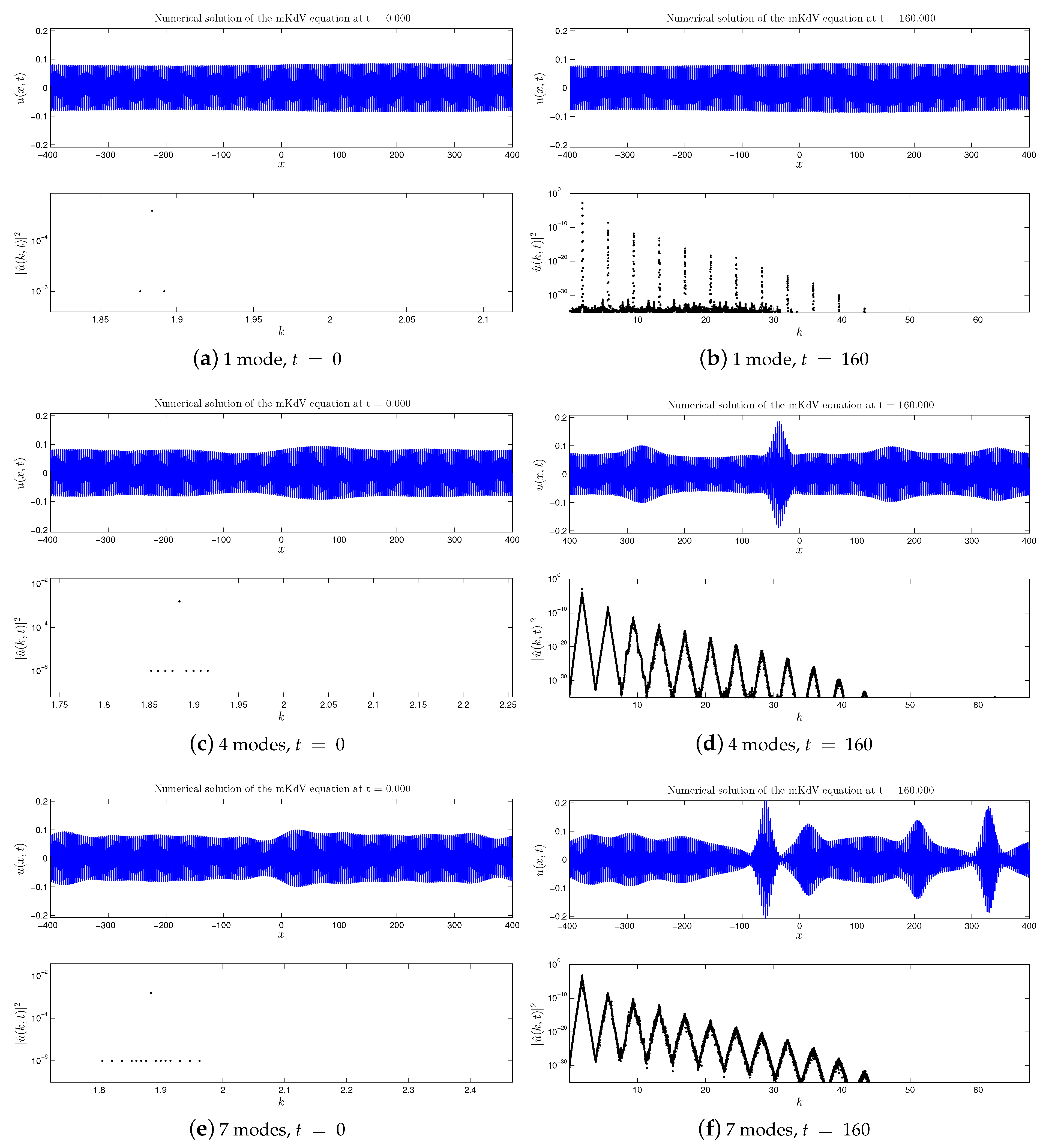
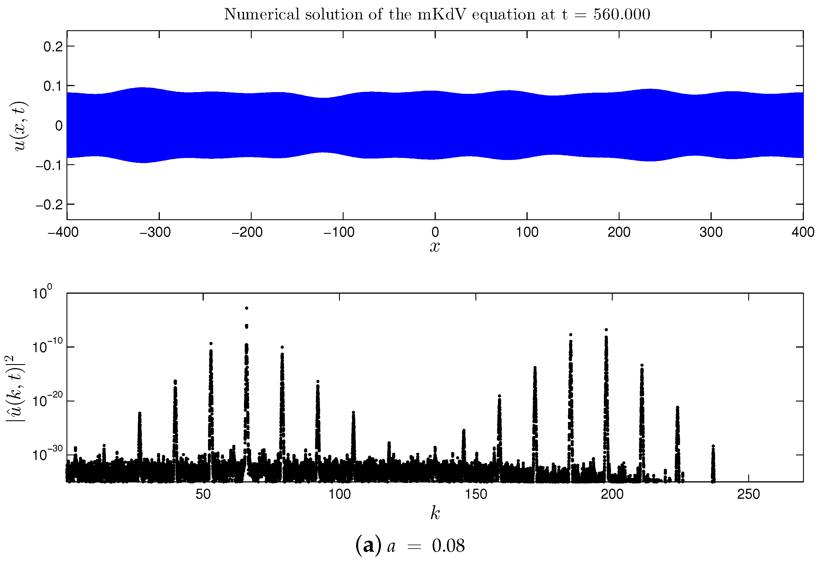
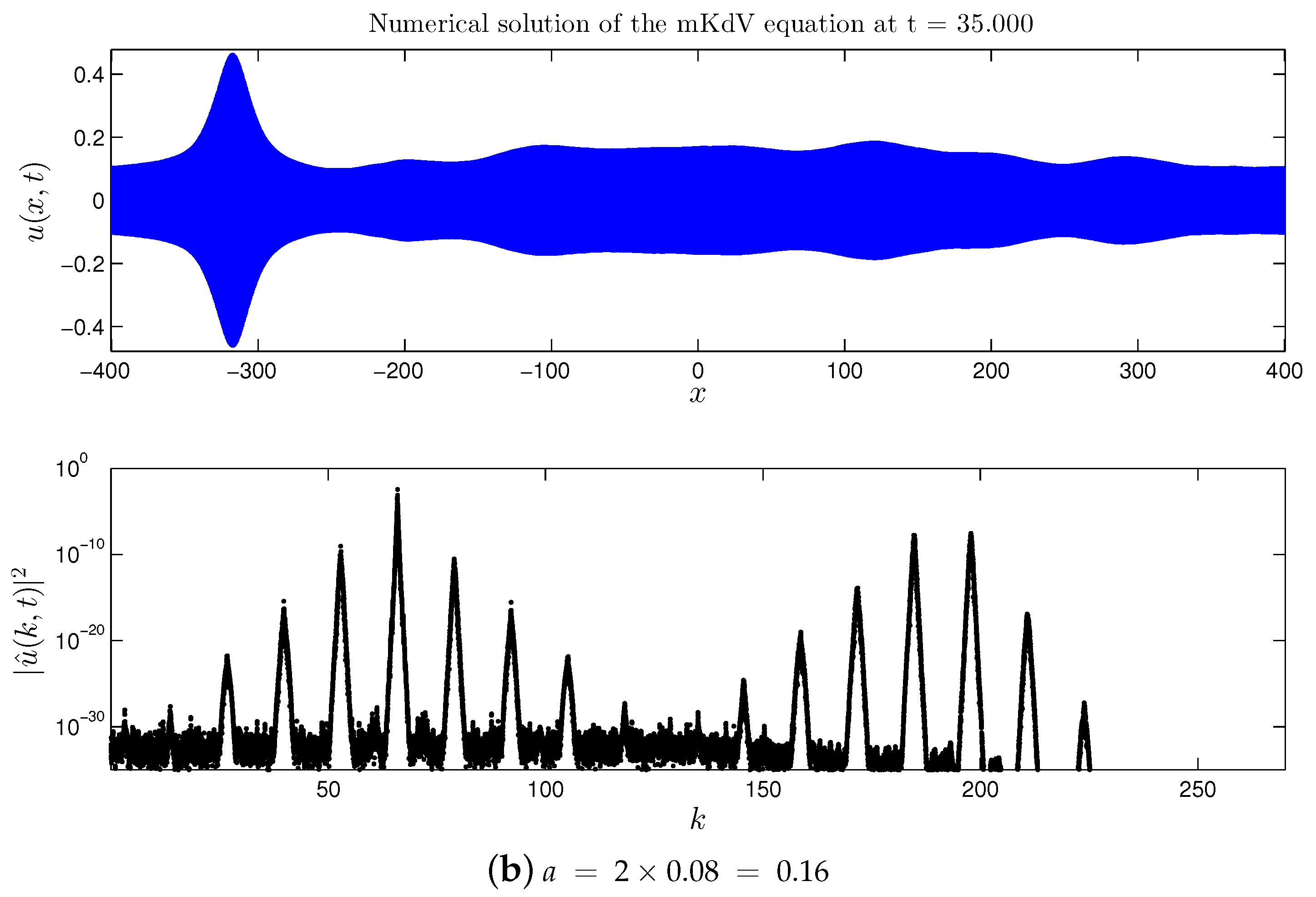
2. mKdV Equation With Broad Spectrum Initial Perturbation

In order to investigate the broader perturbations we considered the following set of numerical experiments which generalize those presented in [16,17]. Here again, in order to solve numerically the mKdV equation on a periodic domain we use the classical Fourier-type pseudo-spectral method [32,33]. All the derivatives are computed in the Fourier space, while all the nonlinear products are performed in the physical space (with the linear CPU-time, i.e., $\mathcal{O}\left(N\right)$, where N is the number of collocation points necessarily equal to the number of Fourier modes). Thanks to the FFT algorithm [34,35,36] the passage between these two representations is done in the super-linear time $\mathcal{O}(Nlog(N\left)\right)$, which determines the overall algorithm complexity (per time step) $\mathcal{O}(mNlog(N\left)\right)$, $m\sim 1$ being the number of FFTs needed to evaluate the right-hand side. For the de-aliasing we used the classical $2/3$-rule [33] which was combined (when necessary) with the Fourier smoothing method proposed in [37] for more delicate treatment of higher frequencies. The discretization in time was done with the embedded adaptive 5th order Cash–Karp Runge–Kutta scheme [38] with the adaptive PI step size control [39]. We note that for the numerical simulation of the gKdV equation one needs to set more stringent tolerances, because of the presence of highly nonlinear products. The accuracy of dynamical computations was checked by following, for example, the $L_2$ norm of the solution $u(x,t)$ which is one of the invariants of the (g,m)KdV dynamics. In all the experiments this norm was conserved up to the 8th digit with smaller oscillations around the mean value.

2.1. Direct cascade

The numerical set-up used in this study is a direct generalization of the test case used also earlier in [40]. We consider the following initial condition posed on a periodic domain $[-\ell ,\ell ]=\left[-\pi /k_0,\pi /k_0\right]$:

$$u(x,0)\equiv u_0\left(x\right)=a\left(1+\delta \sum _{j}sin\left(j{K}_{0}x\right)\right)sin\left(k_{0}x\right),$$

(4)

where a is the base wave amplitude, $\delta$ is the perturbation magnitude and the wavenumbers $k_0$, $K_0$ and j are chosen such that their ratio $k_0/\left(j{K}_0\right)\in \mathbb{Z}$. The last constraint comes from the periodicity conditions on the initial data. Moreover, the spectral gap between the base wave $k_0$ and its modulation $K_0$ contains two orders of magnitude (see

Table 1. Various parameters used in simulations of the direct energy cascade subject to a broad excitation.

Base wave amplitude, a	$0.08$
Perturbation magnitude, $\delta$	$0.05$
Base wavenumber, $k_0$	$1.884$
Perturbation wavenumber, $K_0$	$0.00785$
Ratio of wavelengths, $k_0/K_0$	240
Number of Fourier modes, N	16 384

for the values of parameters). When we perturb the base wave according to (4) with a few modes we have to keep in mind that the perturbation has to be different from the base wave at least with one order of magnitude. Taking into account this constraint along with $k_0/\left(j{K}_0\right)\in \mathbb{Z}$, we obtain that for our numerical set-up j is roughly limited by 10.

The case $j\equiv 1$ corresponds to the computations already discussed in [16,17,40]. The values of parameters are given in the Table 1. In Figure 1 (left panels (a,c,e)) we show the corresponding perturbed initial conditions. The case Figure 1a corresponds to $j=1$. The Fourier spectrum on the bottom panel shows three points which correspond to the base wave $k_0$ (the most energetic mode) and two side bands $k_0\pm K_0$. On Figure 1c, we depict the perturbation by $k_0\pm K_0$, $k_0\pm 2K_0$, $k_0\pm 3K_0$ and $k_0\pm 4K_0$ modes (in total nine points on the bottom panel). Finally, the last Figure 1e corresponds to $j=1$, 2, 3, 4, 6, 8 and 10 (counting 15 modes in total).

The evolution of three initial conditions from Figure 1 (left panels) is simulated using the mKdV Equation (2). The numerical snapshots taken at the same moment of time $t=160.0$ are shown on Figure 1 (right panels). It can be readily seen that the nonlinear stage of the MI develops much faster if the initial perturbation contains more spectral modes. For instance, the first initial condition with $j=1$ unstable mode shows some signs of the MI. Namely, the cascading modes are already present in the Fourier domain. However, their broadening is not developed yet. It is translated to the physical space by the absence of any amplification of the base wave, while on Figure 1d,f the MI is fully developed with amplification factors up to two times.

In order to show that the MI can be fully developed even from a single perturbation mode we present a numerical snapshot on Figure 2a corresponding to the initial condition depicted at Figure 1a but taken at the moment of time $t=620.0$. A comparable amplification is achieved. However, it happens almost four times slower than for initial conditions shown in Figure 1c,e.

This series of numerical experiments shows that a broader initial perturbation not only does not suppress the dynamical energy cascade, but also the position of all the cascading modes is not affected. The cascade shape remains exponential and it was studied in details (in the case $j=1$) in [16,17]. We performed the same battery of tests for numerous perturbative modes (see Figure 1c,e) and with double initial amplitude (thus, double initial wave steepness). In this study we show only one snapshot corresponding to seven spectral modes and the initial amplitude $a=0.16=2\times 0.08$. Despite the violent MI observed in this picture (Figure 2b, upper panel) the structure of the cascade still can be recognized, even if some deviation from the exponential shape can be recognized.

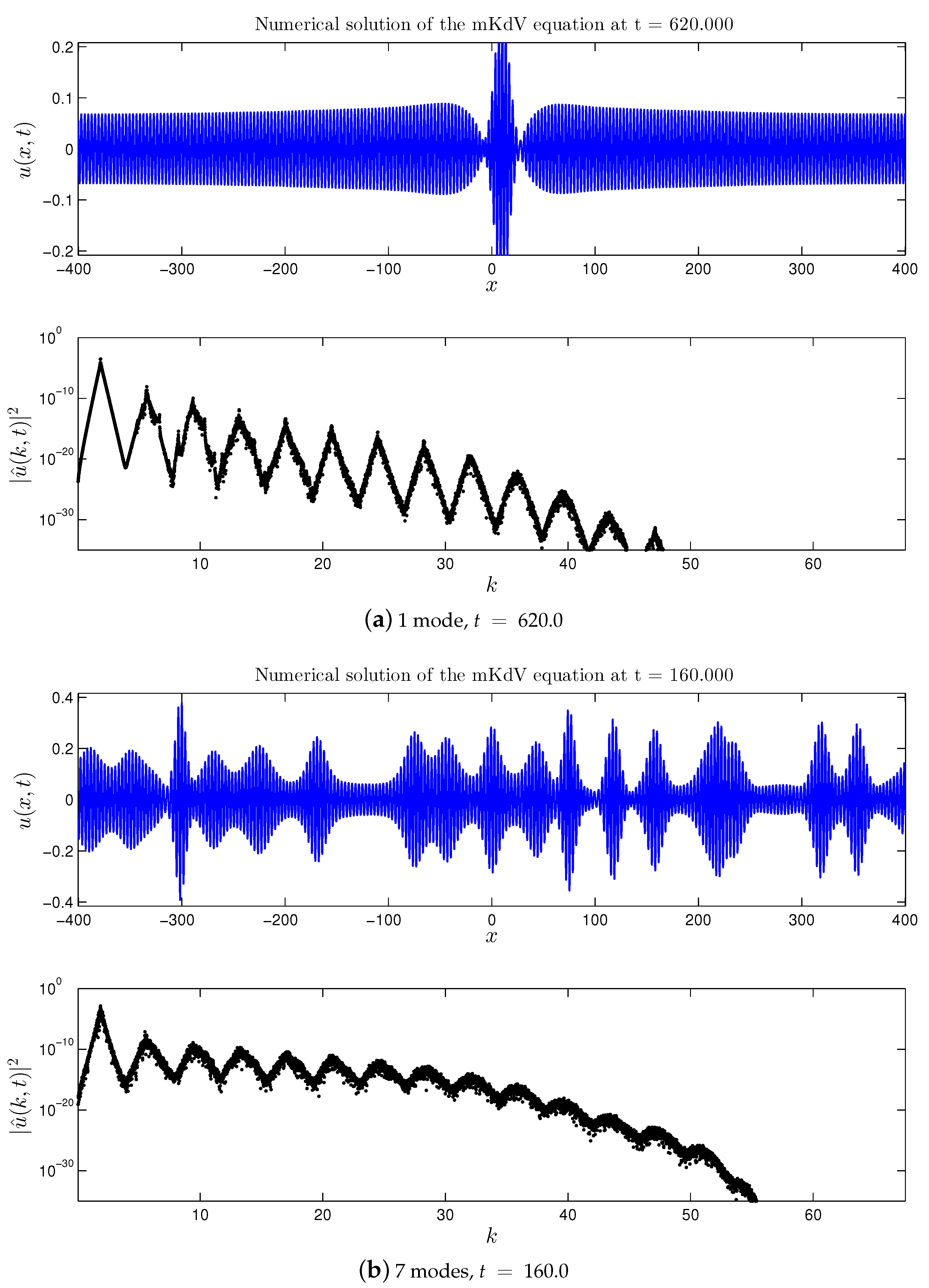
2.2. Double Cascade

As it was demonstrated in [17] for the mKdV Equation (2), a shift in the base mode in Fourier space towards higher frequencies can lead to the formation of a double energy cascade (that is, the simultaneous appearance of the direct and inverse energy cascades). As in the case of the direct cascade, the experiments were performed with only one unstable mode. In this study we enrich the perturbation with up to seven spectral modes in order to see whether this double cascade can still be observed in such extreme conditions.

The numerical parameters for this series of experiments are provided in

Table 2. Various parameters used in simulations of the double energy cascade subject to a broad excitation.

Base wave amplitude, a	$0.08$
Perturbation magnitude, $\delta$	$0.05$
Base wavenumber, $k_0$	$35\times 1.884$
Perturbation wavenumber, $K_0$	$0.00785$
Ratio of wavelengths, $k_0/K_0$	240
Number of Fourier modes, N	$2\times 16$ 384

. In the previous work [17] it was noticed that the increase in the spectral domain yields the appearance of a second occurrence of the double energy cascade. Consequently, we studied several sizes of the computational spectral domain. Here we report the results for $N=2\times$ 16,384 in order to demonstrate the formation of the double cascade along with its repetition in two occurrences if the spectral domain can host them.

The corresponding results are shown on Figure 3 for the initial time $t=0$ (panel (a)), $t=5.0$ (panel (b)) and the same time $t=160.0$ (panel (c)) as in experiments reported above.

As a conclusion, we observe that the double cascade appears almost immediately (see Figure 3b, lower panel) corresponding to $t=5.0$) and it is accompanied by a fully developed MI in the physical space (see Figure 3b, upper panel). The comparison of the present results with previous numerical results [17] shows that even the location of cascading modes appears to be the same up to the graphical resolution.

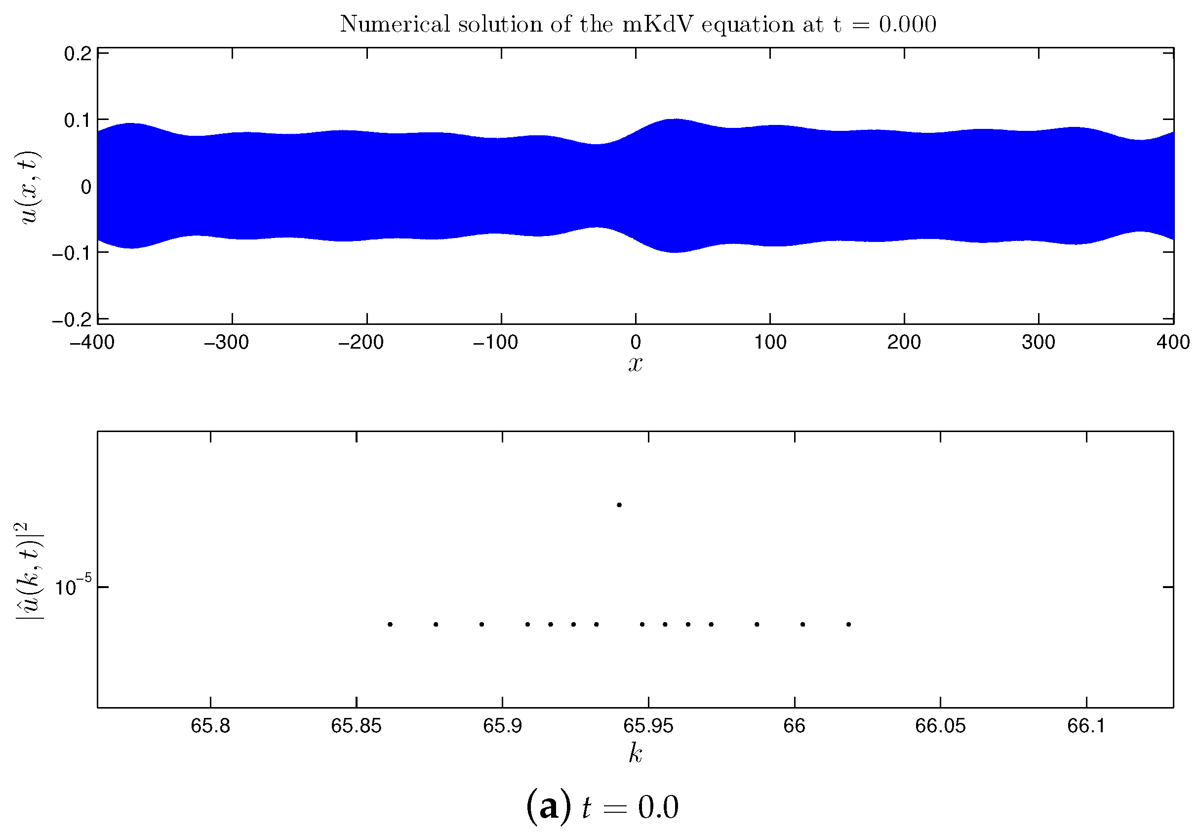
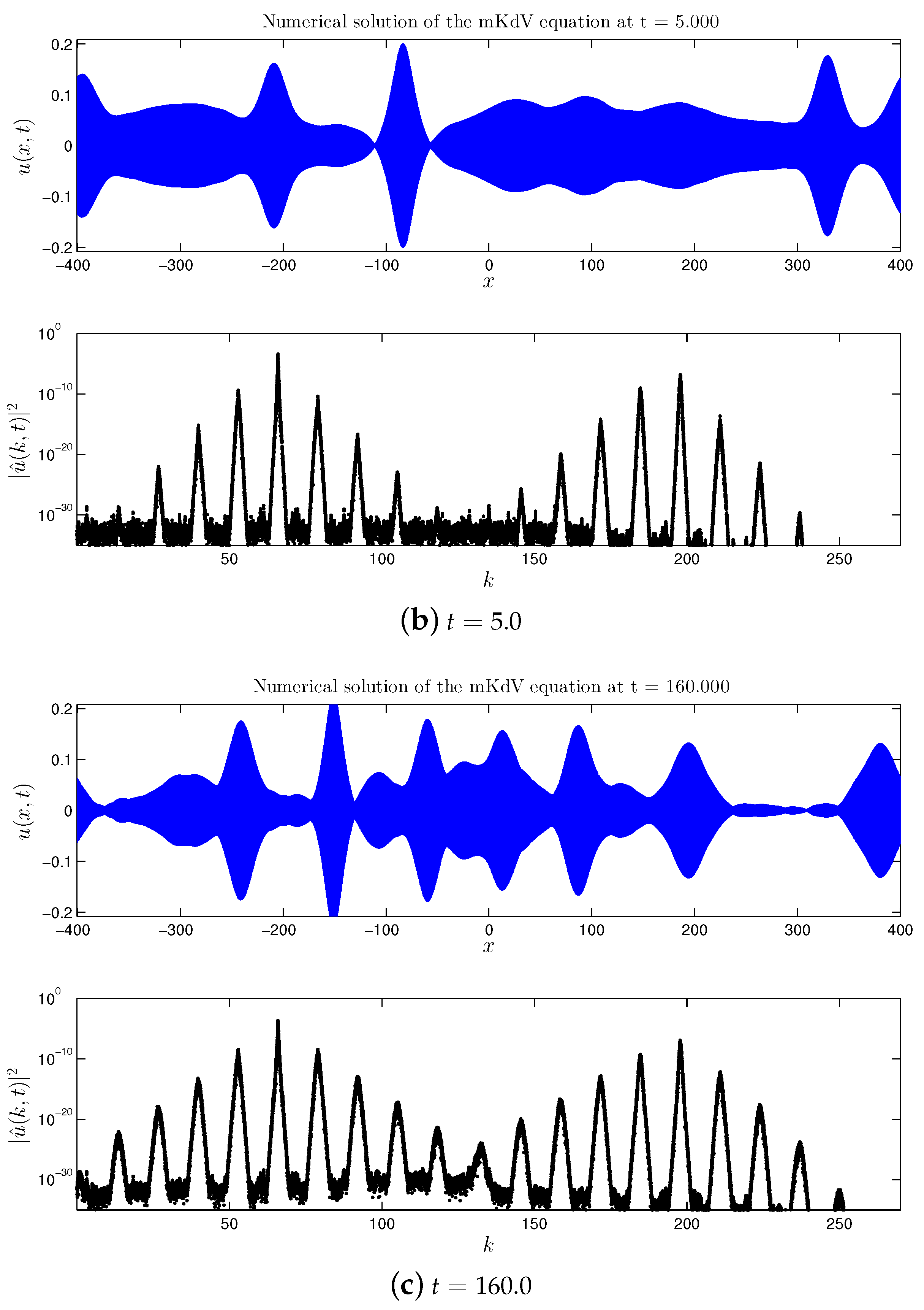
3. Quartic and Quintic gKdV Equations

In this Section we will consider the following particular gKdV Equation (3) where we keep only quartic ($\alpha \equiv 0$, $\beta \equiv 0$, $\delta >0$, $\gamma \equiv 0$) or quintic ($\alpha \equiv 0$, $\beta \equiv 0$, $\delta \equiv 0$, $\gamma >0$) nonlinearities:

$$\begin{array}{ccc}\hfill \mathrm{quartic}\mathrm{KdV}\left(u\right)& \doteq & u_t+u_{xxx}+\delta u^3{u}_x=0,\hfill \end{array}$$

(5)

$$\begin{array}{ccc}\hfill \mathrm{quintic}\mathrm{KdV}\left(u\right)& \doteq & u_t+u_{xxx}+\gamma u^4{u}_x=0.\hfill \end{array}$$

(6)

Our main goals are:

• Investigate the existence of the direct and inverse energy cascades
• If they exist:

  -

  To compare their formation time scales;

  -

  To compare their structure, i.e., the number of cascading modes, their location, spacing, etc.

In order to meet these goals we will take the same numerical set-up as described above for the direct and double cascades correspondingly (see Table 1 and Table 2). The initial perturbations contain one, four or seven modes as it is shown on Figure 1 (left panels (a,c,e)). Several dozens of computations have been performed for each of two Equations (5) and (6). Below we will show the main findings.

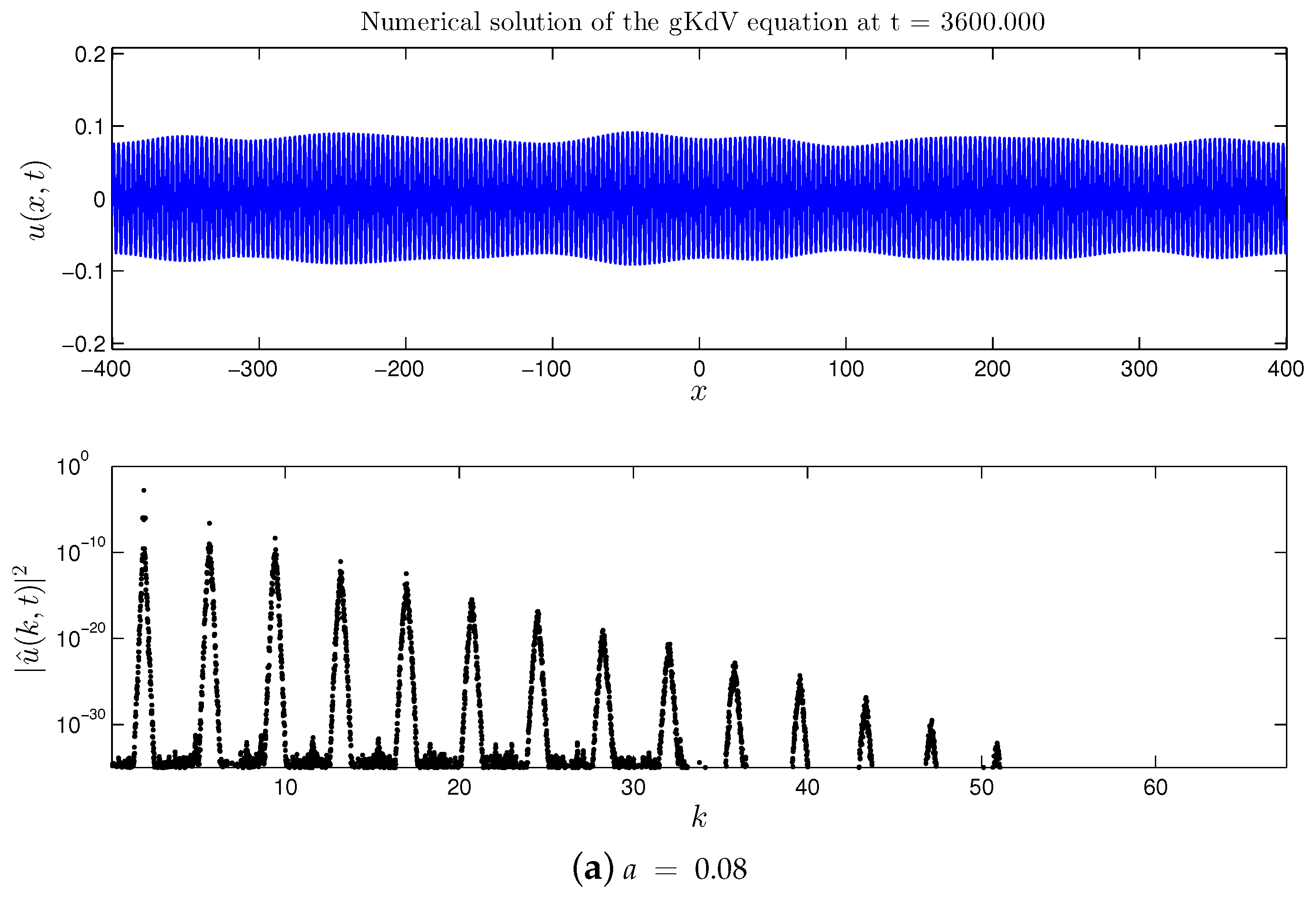
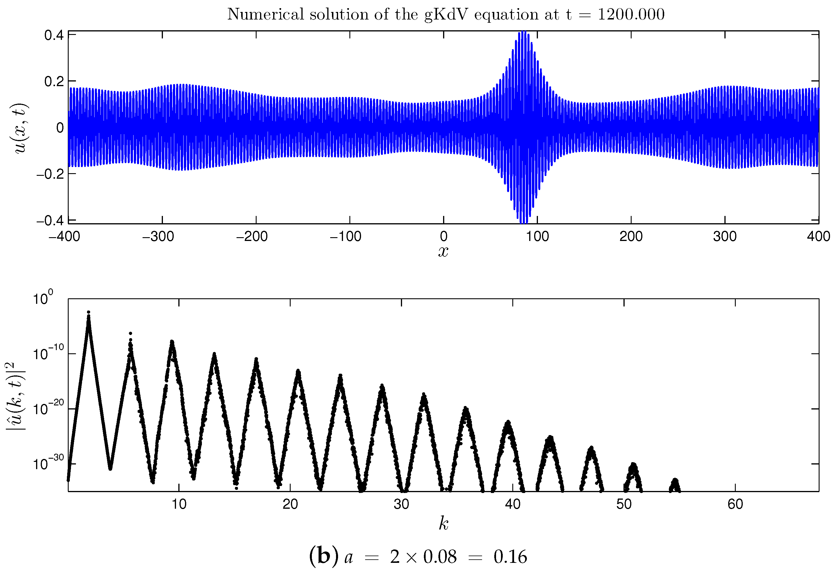
3.1. Quartic gKdV Equation

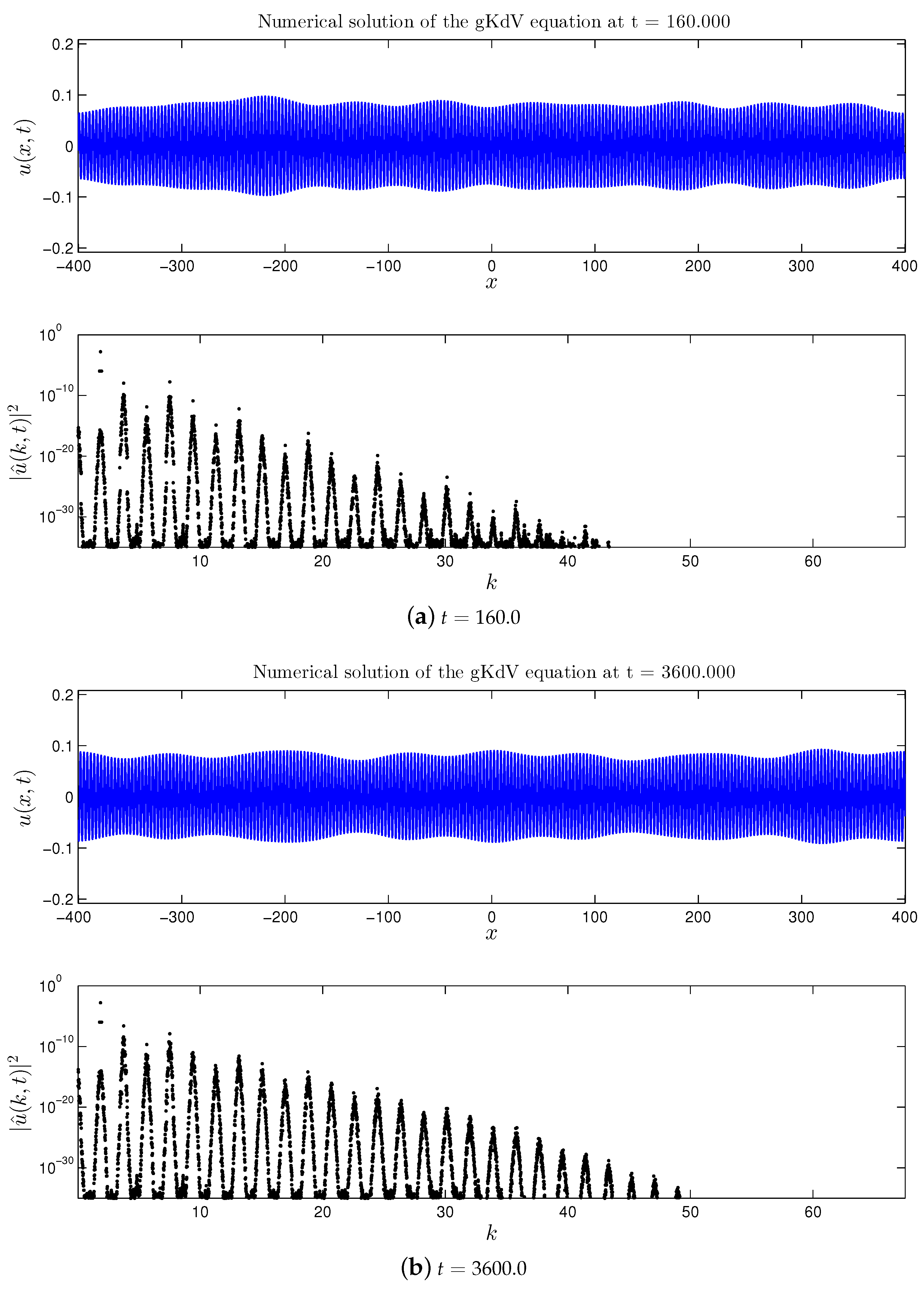
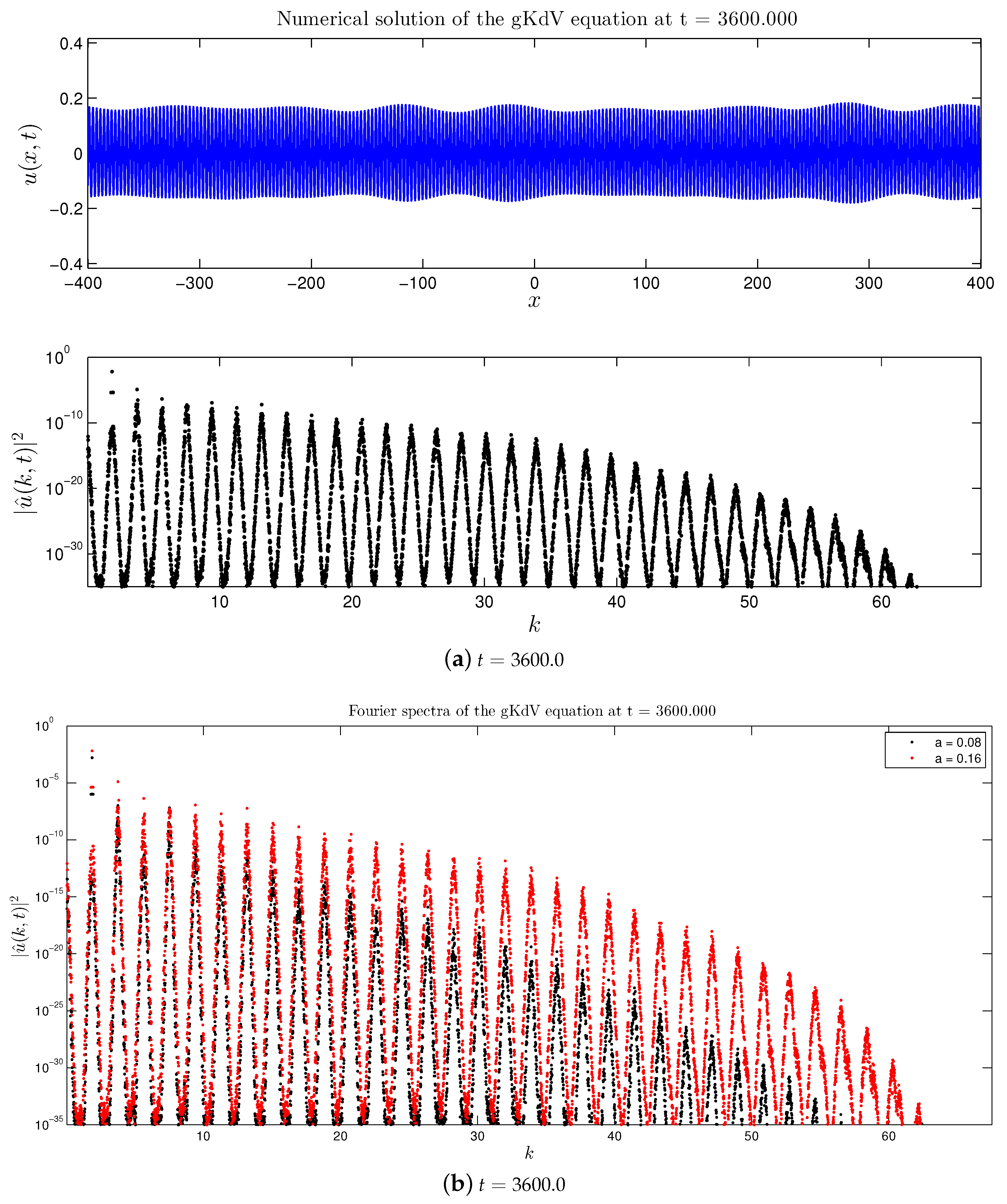
3.1.1. Direct Cascade

The selected results of our numerical simulations are shown on Figure 4 for the initial condition consisting of seven perturbative modes and the base wave amplitude $a=0.08$. This choice of parameters comes from the fact that we would like to highlight the differences with the mKdV Equation (2). The upper pane of Figure 4a shows the time moment $t=160.0$, while Figure 4b reports the system state at $t=3600.0$. We can see that during the system evolution new cascading modes appear in the Fourier spectrum tail (high frequencies). The structure and location of peaks remain the same, while their magnitudes can slightly grow with time.

However, there exist an important qualitative difference with the mKdV case reported in the previous Section. Namely, even at $t=160.0$ (with all other equal parameters and the initial perturbation) the physical space of the mKdV equation already demonstrates the nonlinear stage of the MI development (see Figure 1b,c). On the other hand, the quartic gKdV even for $t=3600.0$ (more than twenty times longer!) does not show any signs of the amplification in the physical space (see Figure 4).

In order to show that the nonlinear MI stage does not occur in the quartic gKdV equation, we performed an additional series of the experiments with higher base wave amplitude. In Figure 5a we show the physical and Fourier spaces for the case of double initial amplitude $a=2\times 0.08=0.16$, while in the lower panel of Figure 5b we show simultaneously Fourier spectra for the simple and double amplitudes at $t=3600.0$. As in previous cases, one can see that there is no significant solution amplification in the physical space. Concerning the Fourier space, the superposition shown on Figure 5b clearly shows the coincidence of the cascading modes locations, while new high frequency cascading modes appear. We note that the Fourier spectrum shown with red dots contains roughly speaking four times more energy (since the initial amplitude is doubled). However, this extra energy is mainly redistributed towards the appearance of new peaks in the tail of the Fourier spectrum, by conserving the energy of several first cascading modes at the long waves end of the spectrum.

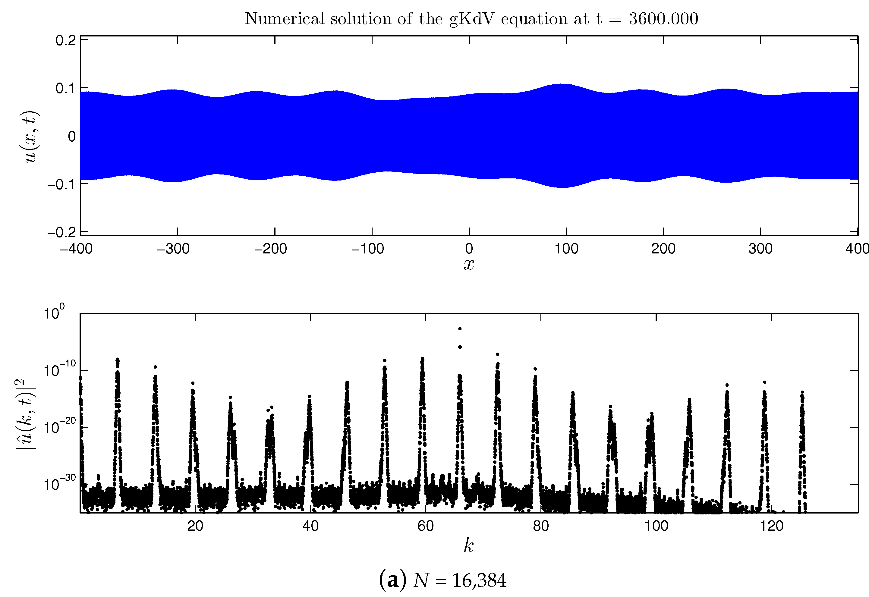
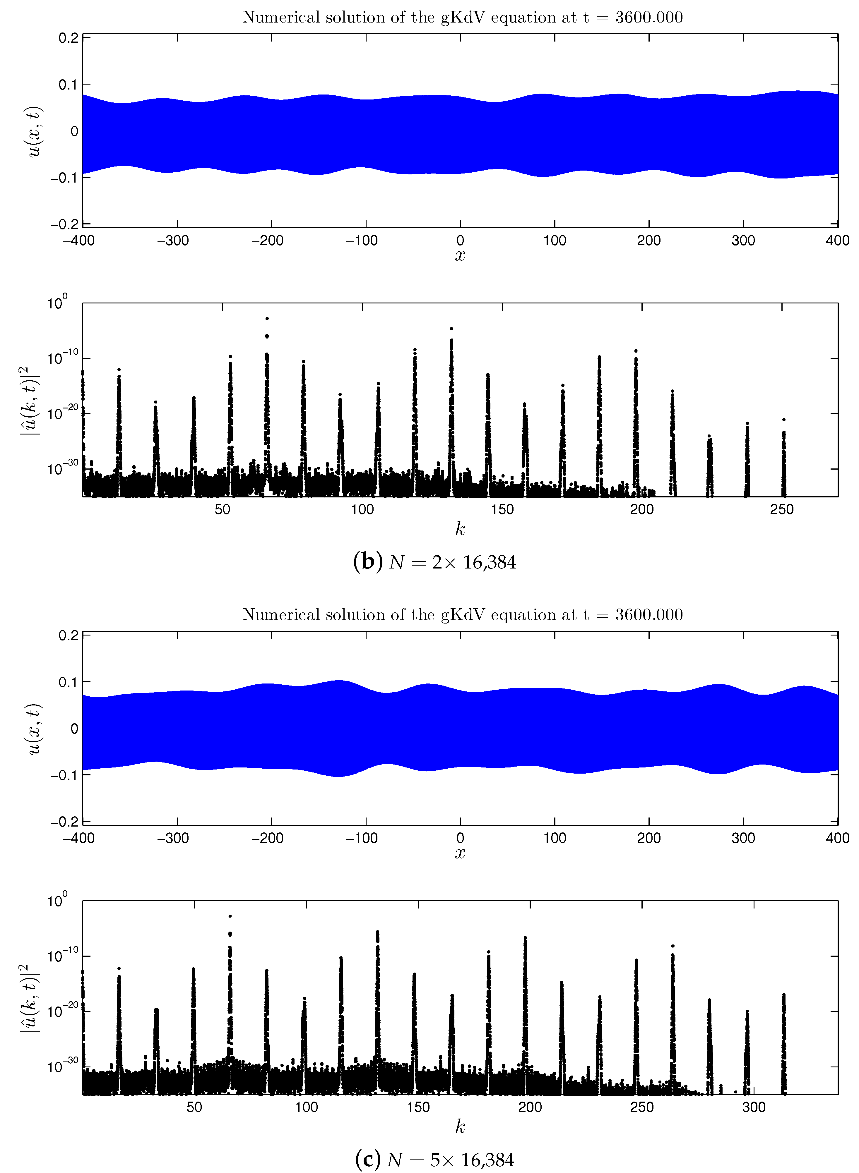
3.1.2. Double Cascade

Numerical experiments to study the double energy cascade formation in the quartic gKdV equation were performed similarly to the study of the mKdV equation reported in the previous section. The main conclusions are the same as for the direct cascade. Namely, in the physical space we do not witness any significant amplification of the base wave.

On the other hand, in the Fourier space several entities of the double cascade are formed. The very interesting fact is that the choice of the spectral domain influences the shape of the double cascade for the quartic gKdV equation. In each spectral domain the total number of cascading modes remains invariant (in the particular case under consideration this number is equal to 19 modes). However, the energy distribution among these modes is different and actually depends on the size of the spectral domain. As we observed in [17], the spectral domain consisting of $N=2\times$ 16,384 Fourier modes can host one entity of the double cascade, while doubling the size of the spectral domain yields logically the appearance of two entities of the cascade (with the total number of cascading modes being 14 in that computation). In order to illustrate this fact for the quartic gKdV equation as well, on Figure 6 we show the formed double cascade for different sizes of the spectral domain.

All pictures are taken at $t=3600.0$, even though the location of the modes and the distribution of energy among them is already clearly visible at $t=60.0$. Longer simulations are necessary in order to show that we do not observe any nonlinear development of the MI in the physical space on the longer horizon. The effect of the energy redistribution in the spectral domain deserves a separate study. It will be performed elsewhere.

3.2. Quintic gKdV Equation

The numerical set-up in this Section is precisely the same as above. However, here we focus on the quintic gKdV Equation (6) with parameter $\mu =6.0$.

The time evolution under the quintic gKdV equation dynamics (6) is totally different from what we observed for the quartic gKdV (5). Namely, in the quintic case a well-developed MI can be observed both in Fourier and physical spaces with physical amplifications of the base wave amplitude going up to two times and higher.

On the other hand, these numerical results are qualitatively the same as for the mKdV Equation (2) reported above and in [16,17]. Namely, the direct and double cascades are accompanied by the nonlinear stage of the MI in the physical space. It can be qualitatively observed on Figure 7b. An interesting difference with the mKdV consists in the appearance of the instability threshold in the quintic gKdV Equation (6). Below this supposed instability threshold the quintic gKdV behaves similarly to the quartic gKdV equation in the physical space. It is manifested by the long time dynamics of the modulated solution in the physical space without the development of the nonlinear stage of the MI (see Figure 7a). In contrast, when we take the doubled initial base wave amplitude $a=2\times 0.08=0.16$, the MI in the physical space is well developed already at $t=1200.0$ as it can be seen on Figure 7b.

Concerning the Fourier space, the number of cascading modes, the spacing between them and the shape of the energy spectrum is preserved regardless the base wave amplitude (below or above the instability threshold, see Figure 7). In contrast to the double cascade, the increase in the spectral domain does not lead to the redistribution of the energy among cascading modes. We do not provide the corresponding pictures here. They can be obtained from the authors after a simple request.

For the double cascade in the quintic gKdV we observe the same entities as in the mKdV equation (see Figure 3 and also [17]). However, what is new is the presence of the instability threshold as it was explained for the direct cascade. In order to see the difference the reader can compare Figure 8a,b.

4. Discussion

In the present study we investigated several KdV-type equations involving higher order nonlinearities. The main focus was on the formation and properties of the dynamical energy cascade in the Fourier space. The second goal was to describe the cases when the formation of this cascade is accompanied by the nonlinear stage of the MI development in the physical space. This question is of capital importance since the nonlinear stage implies important wave amplifications which are put forward nowadays as one of the main physical mechanisms of the freak wave formation [41]. Since, the total number of numerical experiments performed in this study exceeded a few hundreds, we included only the most typical ones.

• First of all, we extended the study of the mKdV equation presented in [16,17] for the case of a broader initial perturbation of the base wave. It was found that previous findings can be transposed to this case as well: formation of the direct and double cascades, their structure is preserved and appears to be quite stable. However, in the broad perturbation case all nonlinear processes are accelerated (i.e., they develop in shorter times).
• Not only the general structure of the energy cascade is preserved, but also the number of the cascading modes (for the fixed spectral domain and the base wave amplitude) and their location in the Fourier space.
• The main difference between the direct and double cascades consists in the fact that the change of the size of the spectral domain does not induce the energy redistribution in the direct cascade, while it changes completely the number of entities, and thus the energy distribution, in the double cascade(s).
• In all the mKdV cases, the formation of dynamical cascades is accompanied by the nonlinear stage of the MI development and the substantial amplification of the base wave in the physical space.
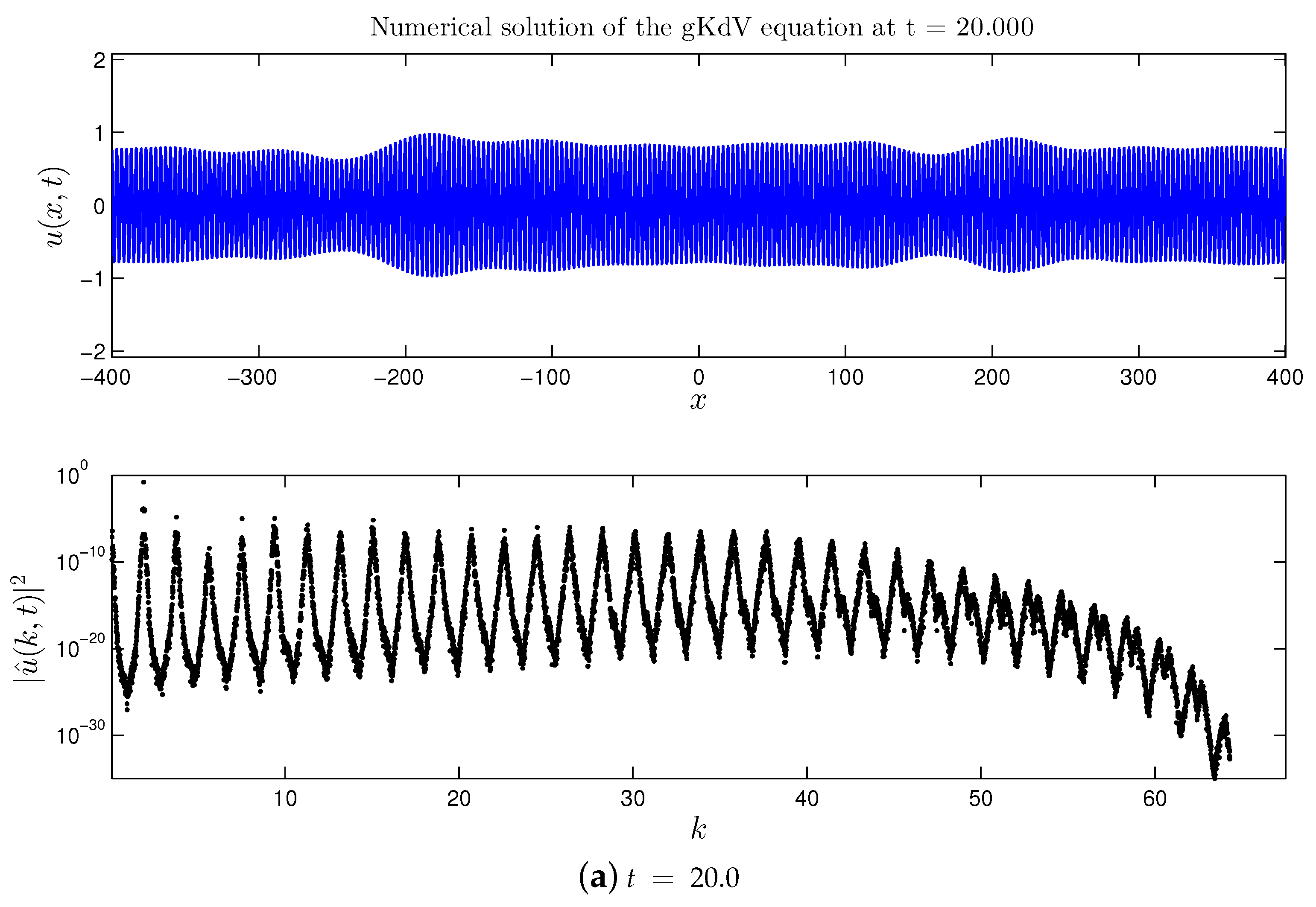
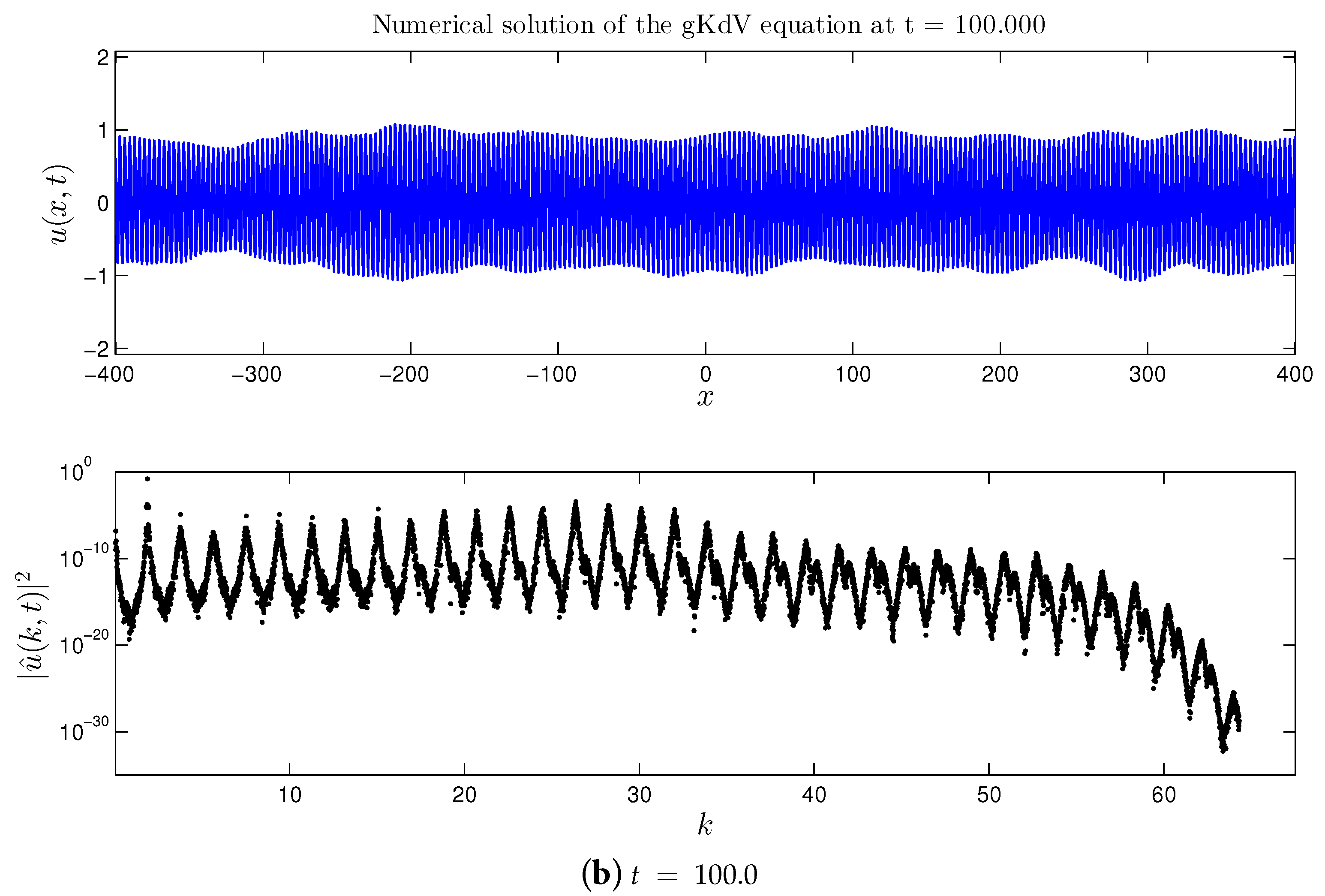
• In the case of the quartic gKdV equation, all the results about the dynamical cascades formation in the spectral domain remain the same. However, no amplification of the base wave amplitude was observed in the physical space.
• The quintic gKdV case is mostly similar to the mKdV equation (with positive nonlinearity) except for the presence of the amplitude threshold in the physical space, below which the amplification does not occur on the time horizons investigated in this study. However, if the amplitude is taken above this threshold, the base wave amplification occurs on longer time scales (virtually three times slower than in mKdV for the parameters considered in this study).

The main findings are summarized in a compact form in

Table 3. The main conclusions of this study summarized in this table. The sign ‘−’ designates the absence of the corresponding property, while ‘+’ means its presence.

Property/Model	KdV (1)	mKdV (2)	Quartic gKdV (5)	Quintic gKdV (6)
Nonlinear Term	${\mathit{uu}}_{\mathit{x}}$	${\mathit{u}}^{\mathbf{2}}{\mathit{u}}_{\mathit{x}}$	${\mathit{u}}^{\mathbf{3}}{\mathit{u}}_{\mathit{x}}$	${\mathit{u}}^{\mathbf{4}}{\mathit{u}}_{\mathit{x}}$
MI	−	+	−	+
Direct cascade	−	+	+	+
Inverse cascade	−	−	−	−
Double cascade	−	+	+	+
Energy redistrib.	−	+	+	+
MI nonlin. stage	−	+	−	+
(amplif. $>2a$)
Threshold	−	−	−	+

.

Strictly speaking the theory of the dynamical energy cascade [5,16] as well as the model equations considered above are valid at best only for moderate nonlinearities $\epsilon \sim \mathcal{O}\left({10}^{-1}\right)$. However, one can ask a legitimate question: what happens if we push the nonlinearity in the wave system to the finite size $\sim \mathcal{O}\left(1\right)$ as in the strong turbulence? For this purpose we performed an additional experiment for the quartic KdV Equation (5) with the base wave amplitude $a=10\times 0.08=0.8$. Together with seven perturbative modes the initial condition reaches $\epsilon \sim \mathcal{O}\left(1\right)$ announced above. Two numerical snapshots are shown on Figure 9. First of all, one can notice that there is no visible difference between $t=20.0$ depicted on the upper panel and $t=100.0$ shown below. It means that the fully developed quasi-stationary stage is reached on times $T\sim \mathcal{O}\left(1\right)$. However, most surprisingly even for such a strong nonlinearity one can still recognize the presence of the direct dynamic energy cascade, despite the fact that we step out from all reasonable ranges of model and theory applicability.

Recently obtained theoretical results, presented in [12,42], indicate some direction for further studies in order to be able to interpret in detail the available results of numerical simulations and get answers to at least some of the open questions. So, the modulation instability for the Korteweg–de Vries (KdV)-family of equations

$$u_t+s{u}^p{u}_x+u_{xxx}=0,$$

(7)

with $s=\pm 1$ and $p>0$ being an arbitrary integer, has been studied in [42]. As modulation instability is defined for the NLS-type of equation, the main question was to deduce an envelope equation for the KdV-family (7). It was proven that general form of envelope equations is different for $p=2n$ (symmetric case) and for $p=2n-1$ (asymmetric case). Moreover, in the latter case the coefficients of the envelope equations depend explicitly on a numerical factor (called pedestal) which in turn is defined by the parameters of initial excitation. This is in accordance with our results demonstrating substantial difference between quartic and quintic cases. A relation between cascades, which might appear in these two families of equations, is presently under study. This is a highly nontrivial fact due to many reasons (different definitions for the small parameter, different dependencies of the cascade form, its very appearance on the parameters of initial excitation, etc.).

The coefficients of the envelope equations have been deduced explicitly in [12] and key characteristics of the modulation instability (that is, the instability increment, its maximum, boundary and maximal wave numbers) were written out. Again, the clear difference between symmetric and asymmetric cases has been demonstrated. In particular, the increment of instability in the latter case depends on the initial conditions in a way which assumes the existence of a lower threshold needed for the developing of instability (see [12] (Equation (57))). This is in agreement with our conclusions.

Summarizing, these novel theoretical results might be useful for planning numerical and laboratory experiments and for explaining the available data. An important issue here would be to choose small parameters and initial amplitudes facilitating these results which is not a simple problem (cf., [12]).

The results presented in this study show that nonlinear stages of the MI are highly structured at the level of the Fourier power spectrum. This gives us the hope that such processes can be effectively described by reduced order models obtained with finite mode truncations of Galerkin type. The reduction of model complexity will allow us to avoid the systematic application of Direct Numerical Simulations (DNS). This method has been effectively applied to strong turbulence in e.g., [43] and to discrete WTT in [44]. However, it is well known that the Galerkin method gives good accuracy of calculations only for smooth solutions. As it can be seen from all the figures presented in our work (on the) upper panels for the physical space and lower panels for Fourier spectra), the numerical solutions to our problem (a solution arising from the modulation instability) is not a smooth function. For instance, our solutions show quite wild behaviour in the physical space. Moreover, they have an essentially discrete Fourier spectra (in contrast to the WTT where the spectra are continuous). Consequently, the application of the discrete Galerkin method could be envisioned here. However, the choice of appropriate eigenfunctions basis for higher KdV-type equations is an open question. That is why the application of finite mode truncations still remains unexplored and it deserves a further thorough scientific investigation.

References

- Richardson, L.F. Weather Prediction by Numerical Process; Cambridge University Press: Cambridge, UK, 1922; p. 262. [Google Scholar]
- Kolmogorov, A.N. The Local Structure of Turbulence in Incompressible Viscous Fluid for Very Large Reynolds Numbers. Proc. R. Soc. Lond. A 1991, 434, 9–13. [Google Scholar] [CrossRef]
- Zakharov, V.E.; Lvov, V.S.; Falkovich, G. Kolmogorov Spectra of Turbulence I. Wave Turbulence; Series in Nonlinear Dynamics; Springer: Berlin, Germany, 1992; p. 264. [Google Scholar]
- Kartashova, E. Energy spectra of 2D gravity and capillary waves with narrow frequency band excitation. Europhys. Lett. 2012, 97, 30004. [Google Scholar] [CrossRef]
- Kartashova, E. Energy transport in weakly nonlinear wave systems with narrow frequency band excitation. Phys. Rev. E 2012, 86, 041129. [Google Scholar] [CrossRef] [PubMed]
- Kartashova, E. Time scales and structures of wave interaction exemplified with water waves. Europhys. Lett. 2013, 102, 44005. [Google Scholar] [CrossRef]
- Boussinesq, J.V. Essai sur la théorie des eaux courantes. Mémoires présentés par divers savants à l’Acad. des Sci. Inst. Nat. France 1877, XXIII, 1–680. [Google Scholar]
- Korteweg, D.J.; de Vries, G. On the change of form of long waves advancing in a rectangular canal, and on a new type of long stationary waves. Philos. Mag. 1895, 39, 422–443. [Google Scholar] [CrossRef]
- Marchant, T.R.; Smyth, N.F. The extended Korteweg-de Vries equation and the resonant flow of a fluid over topography. J. Fluid Mech. 1990, 221, 263–287. [Google Scholar] [CrossRef]
- Grimshaw, R. Internal Solitary Waves. In Environmental Stratified Flows; Grimshaw, R., Ed.; Springer: New York, NY, USA, 2002; pp. 1–27. [Google Scholar] [CrossRef]
- Shabat, A.B.; Adler, V.E.; Marikhin, V.G.; Mikhailov, V.V.; Sokolov, V.V. (Eds.) Encyclopedia of Integrable Systems; Landau Institute for Theoretical Physics: Chernogolovka, Russia, 2010; p. 458. [Google Scholar]
- Tobisch, E.; Pelinovsky, E. Constructive Study of Modulational Instability in Higher Order Korteweg-de Vries Equations. Fluids 2019, 4, 54. [Google Scholar] [CrossRef]
- Tao, T. Scattering for the quartic generalised Korteweg-de Vries equation. J. Differ. Equ. 2007, 232, 623–651. [Google Scholar] [CrossRef]
- Bronski, J.C.; Johnson, M.A. The Modulational Instability for a Generalized Korteweg-de Vries Equation. Arch. Ration. Mech. Anal. 2010, 197, 357–400. [Google Scholar] [CrossRef]
- Bronski, J.C.; Johnson, M.A.; Kapitula, T. An index theorem for the stability of periodic travelling waves of Korteweg-de Vries type. Proc. R. Soc. Edinb. Sect. A 2011, 141, 1141–1173. [Google Scholar] [CrossRef]
- Dutykh, D.; Tobisch, E. Direct dynamical energy cascade in the modified KdV equation. Physica D 2015, 297, 76–87. [Google Scholar] [CrossRef]
- Dutykh, D.; Tobisch, E. Observation of the Inverse Energy Cascade in the modified Korteweg-de Vries Equation. Europhys. Lett. 2014, 107, 14001. [Google Scholar] [CrossRef]
- Newell, A.C.; Rumpf, B. Wave Turbulence. Ann. Rev. Fluid Mech. 2011, 43, 59–78. [Google Scholar] [CrossRef]
- Janssen, P.A.E.M. Nonlinear four-wave interactions and freak waves. Phys. Oceanogr. 2003, 33, 863–884. [Google Scholar] [CrossRef]
- Tobisch, E. Energy spectrum of ensemble of weakly nonlinear gravity-capillary waves on a fluid surface. J. Exp. Theor. Phys. 2014, 119, 359–365. [Google Scholar] [CrossRef]
- Grimshaw, R.; Pelinovsky, D.E.; Pelinovsky, E.N.; Talipova, T. Wave group dynamics in weakly nonlinear long-wave models. Physica D 2001, 159, 35–57. [Google Scholar] [CrossRef]
- Dullin, H.R.; Gottwald, G.A.; Holm, D.D. On asymptotically equivalent shallow water wave equations. Physica D 2004, 190, 1–14. [Google Scholar] [CrossRef]
- Zabusky, N.J.; Galvin, C.C.J. Shallow Water Waves, the Korteweg-de Vries Equation and Solitons. J. Fluid Mech. 1971, 47, 811–824. [Google Scholar] [CrossRef]
- Johnson, R.S. Camassa-Holm, Korteweg-de Vries and related models for water waves. J. Fluid Mech. 2002, 455, 63–82. [Google Scholar] [CrossRef]
- Schamel, H. A modified Korteweg-de Vries equation for ion acoustic wavess due to resonant electrons. J. Plasma Phys. 1973, 9, 377–387. [Google Scholar] [CrossRef]
- Toida, M.; Ohsawa, Y. KdV Equations for High- and Low-Frequency Magnetosonic Waves in a Multi-Ion Plasma. J. Phys. Soc. Jpn. 1994, 63, 573–582. [Google Scholar] [CrossRef]
- Nakamura, Y.; Bailung, H.; Shukla, P.K. Observation of Ion-Acoustic Shocks in a Dusty Plasma. Phys. Rev. Lett. 1999, 83, 1602–1605. [Google Scholar] [CrossRef]
- Grue, J.; Jensen, A.; Rusas, P.O.; Sveen, J.K. Properties of large-amplitude internal waves. J. Fluid Mech. 1999, 380, 257–278. [Google Scholar] [CrossRef]
- Whitfield, A.J.; Johnson, E.R. Rotation-induced nonlinear wavepackets in internal waves. Phys. Fluids 2014, 26, 056606. [Google Scholar] [CrossRef]
- Holloway, P.; Pelinovsky, E.; Talipova, T. Internal Tide Transformation and Oceanic Internal Solitary Waves. In Environmental Stratified Flows; Grimshaw, R., Ed.; Kluwer Academic Publishers: Boston, MA, USA, 2003; pp. 29–60. [Google Scholar] [CrossRef]
- Shabat, A.B.; Kartashova, E. Computable integrability. chapter 1: General notions and ideas. arXiv 2005, arXiv:math-ph/0504020. [Google Scholar]
- Boyd, J.P. Chebyshev and Fourier Spectral Methods, 2nd ed.; Dover Publications: New York, NY, USA, 2000; p. 688. [Google Scholar]
- Trefethen, L.N. Spectral Methods in MatLab; Society for Industrial and Applied Mathematics: Philadelphia, PA, USA, 2000; p. 184. [Google Scholar]
- Frigo, M.; Johnson, S.G. FFTW: An adaptive software architecture for the FFT. In Proceedings of the 1998 IEEE International Conference on Acoustics, Speech and Signal Processing, ICASSP ’98 (Cat. No. 98CH36181). Seattle, WA, USA, 15 May 1998; Volume 3, pp. 1381–1384. [Google Scholar]
- Frigo, M. A fast Fourier transform compiler. In Proceedings of the 1999 ACM SIGPLAN Conf. on Programming Language Design and Implementation (PLDI), Atlanta, GA, USA, 1–4 May 1999; Volume 34, pp. 169–180. [Google Scholar]
- Frigo, M.; Johnson, S.G. The Design and Implementation of FFTW3. Proc. IEEE 2005, 93, 216–231. [Google Scholar] [CrossRef]
- Hou, T.Y.; Li, R. Computing nearly singular solutions using pseudo-spectral methods. J. Comput. Phys. 2007, 226, 379–397. [Google Scholar] [CrossRef]
- Cash, J.R.; Karp, A.H. A variable order Runge-Kutta method for initial value problems with rapidly varying right-hand sides. ACM Trans. Math. Softw. 1990, 16, 201–222. [Google Scholar] [CrossRef]
- Hairer, E.; Wanner, G. Solving Ordinary Differential Equations II. Stiff and Differential-Algebraic Problems; Springer Series in Computational Mathematics; Springer: Berlin/Heidelberg, Germany, 1996; Volume 14, p. 614. [Google Scholar]
- Grimshaw, R.; Pelinovsky, E.N.; Talipova, T.; Ruderman, M.S.; Erdelyi, R. Short-Lived Large-Amplitude Pulses in the Nonlinear Long-Wave Model Described by the Modified Korteweg-De Vries Equation. Stud. Appl. Math. 2005, 114, 189–210. [Google Scholar] [CrossRef]
- Onorato, M.; Osborne, A.R.; Serio, M.; Bertone, S. Freak waves in random oceanic sea states. Phys. Rev. Lett. 2001, 86, 5831–5834. [Google Scholar] [CrossRef] [PubMed]
- Tobisch, E.; Pelinovsky, E. Conditions for modulation instability in higher order Korteweg-de Vries equations. Appl. Math. Lett. 2019, 88, 28–32. [Google Scholar] [CrossRef]
- Balajewicz, M.J.; Dowell, E.H.; Noack, B.R. Low-dimensional modelling of high-Reynolds-number shear flows incorporating constraints from the Navier-Stokes equation. J. Fluid Mech. 2013, 729, 285–308. [Google Scholar] [CrossRef]
- Kartashova, E.A. Weakly nonlinear theory of finite-size effects in resonators. Phys. Rev. Lett. 1994, 72, 2013–2016. [Google Scholar] [CrossRef]