1. Objectives and Plan of the Paper
This paper is devoted to develop an approach based on a suitable development of the theory of swarms, arguably initiated by the celebrated paper by Cucker and Smale [
1], applied to behavioral dynamics of social and economic systems with particular focus on the study of price sequences. The behavioral swarm theory approach to the dynamics of prices was recently introduced in [
2] and this present paper aims at providing a deeper insight in the role of cherry picking and asymmetric interactions.
The modeling and simulations of large systems of interacting behavioral entities have been developed by methods of the so-called kinetic theory of active particles, in short KTAP, as well as by recent developments of the theory of swarms. For additional details, the interested reader is addressed to the KTAP approach [
3], to the kinetic theory approach by mean field and Fokker-Plank models [
4], and to the mathematical theory of behavioral swarms [
2,
5]. All approaches refer to large systems of interacting living entities, called active particles, whose state at the microscopic scale, or shortly micro-scale, includes well defined social and/or economic variables which are heterogeneously distributed over active particles.
The common feature of all different kinetic theory methods is that the overall state of the system is described by a distribution function over the micro-state. This distribution accounts for the overall heterogeneity of the system. In the case of behavioral swarms, the overall state of the system is delivered by a whole set of micro-states. An additional common feature is that mathematical models are obtained by inserting into general mathematical structures, which differ for each of the aforementioned approaches, models of the dynamics of interactions. Indeed, this rationale is followed also in our paper.
The KTAP has been applied to model several socio-economic phenomena, among others, propagation of opinion formation and credit risk over networks [
6,
7], idiosyncratic learning [
8], opinion dynamics [
9,
10] and social inequality [
11], while additional bibliography is provided in [
12]. Another example about the use of kinetic theory to explain the market mechanisms is in [
13] where the microscopic description leads to a system of linear Boltzmann-type equations.
An alternative method is the so-called agent-based modeling (ABM). Although not mathematically fully grounded, it is useful to understand complex dynamics. The agents are commonly implemented in software as objects, with internal rules. With the model, it is possible to instantiate a population agent, observing what is emerging by the actions and interactions that produce following their rules. From the formal point of view, ABMs are close to a narrative of reality, thanks to their flexibility. Still, they are also close to a mathematical structure if they adhere to a rigorous representation via computer code [
14,
15,
16].
As stated before, this paper proposes a development and a new vision of the approach proposed in the second part of [
2], where price dynamics within a market was studied by a swarm theory approach. The scientific literature on swarms has been arguably initiated by physicists, while the interest of mathematicians has been boosted by the visionary paper [
1]. An overview of the vast literature on this topic is far beyond the aims of our paper which consists of understanding how the structure delivered by the classical mathematical theory of swarms [
17] can be modified towards the modeling of social and economic systems. The first step is to set the variables that can describe the individual state of the interacting entities. If particles are viewed as agents which carry a certain social variable, for instance a social or political opinion, an analogous structure has been used to study and control the dynamics of the collective behavior of one or more populations [
18,
19]. The concept of topological interactions in swarms has been introduced in [
20], by which interactions occur with a fixed number of individuals rather than with those belonging to an influence domain, and the mathematical formalization was further developed in [
21].
The main objective of our paper consists of a detailed analysis of the role of the asymmetry in the interactions with respect to symmetric interactions, issue that has been recently treated in [
22]. The aforementioned model presented [
2] is enriched with a proper description of sticky prices and the so-called cherry picking, which assumes that—in addition to prices—quality is also an important factor to be considered. In [
23] a useful economic discussion on market coordination by prices is provided. Other useful references are [
24,
25]. An important asymmetry of our work is represented by the stickiness of seller prices, which allows the market prices to stay stable. Stickiness is a crucial characteristic for seller prices, especially when we consider the realistic phenomenon of
cherry picking, as shown in [
26]. The use of this novel modeling structure for micro-economic analyses of the markets has simultaneously two goals: (i) to observe the agent coordination on the two sides of the market and (ii) investigate the effects of the information presence on the quality. Instead, in a classical model, we would have aggregate demand and offer curves related to a unique good in each market.
The presentation is as follows:
Section 2 provides a qualitative description of the behavioral economic systems object of the modeling approach. More in details, of the dynamics of prices under asymmetric interactions.
Section 3 first introduces the concept of cherry picking that is applied to derive two specific models focusing on specific types of asymmetries. Finally, is devoted to simulations and interpretation of the computational results referring to the framework of economic sciences.
Section 4 looks ahead to possible research perspectives induced by a critical analysis of the contents of our paper.
2. Behavioral Dynamics of Prices
Let us consider a market in which
N sellers and
M buyers trade a specific good. According to the kinetic theory of active particles [
27,
28], sellers and buyers can be regarded as functional subsystems (FS). Within each FS, particles (i.e., sellers or buyers) express an activity which is heterogeneously distributed among them. In this specific case, activity variables for sellers and buyers are the
price assigned by each seller for this good and the
price that each buyer accepts to pay for the good, respectively [
2]. We introduce the following notation:
- -
, corresponds to the first functional subsystem (sellers), where each s-firm expresses the price of the product (good) offered for sale.
- -
, corresponds the second functional subsystem (buyers), where each b-buyer expresses the price that he/she accepts to pay.
- -
The variables which define the activities within each FS are given by the vectors
while their corresponding speeds of change are
where if both prices and related speeds are normalized with respect to their highest value at initial time
, we can assume that
and
. The dynamics can, however, generate values which do not belong to these intervals for larger times.
According to this representation,
m-order moments within each FS can be computed by
where first (
) and second (
) order moments provide the expected (or mean) price and variance, respectively, while higher order moments give information on the distortion.
Following the reasonings exposed in [
2], we assume that
- -
Micro-micro interactions take place only across FSs, but not within the same FS. By these interactions, firms and customers adjust the price by direct contacts.
- -
Macro-micro interactions take place within the same FS, but not across different ones. By these interactions, each seller adjusts her/his price according to the mean stream of sellers, while customers adjust the price accounting for the mean stream of buyers.
Let us now introduce the following quantities deemed to model interactions among particles and between particles and FSs:
- -
models the rate at which a seller s interacts with a buyer b;
- -
models the rate at which a buyer b interacts with a seller s;
- -
models the micro-macro interaction rate between a seller s and her/his own FS;
- -
models the micro-macro interaction rate between a buyer b and her/his own FS;
- -
denotes the micro-micro action, which occurs with rate , of a buyer b over a seller s;
- -
denotes the micro-micro action, which occurs with rate , of a seller s over a buyer b;
- -
denotes the micro-macro action, which occurs with rate of the FS of sellers over a seller s;
- -
denotes the micro-macro action, which occurs with rate of the FS of buyers over a buyer b.
Accordingly, the mathematical structure corresponding to the setting given by Equation (
2) in [
2] is as follows:
for
and
. This provides the framework to derive specific models by inserting into Equation (
2) a detailed description of the interactions.
As remarked in [
2], the system presents asymmetries, since the seller prices are public (e.g., advertised price tags), while buyer prices are unknown to the sellers. This feature is taken into account to properly model the interactions terms:
The interaction rates for both micro-micro and macro-micro interactions asymmetrically decay with the distance between the interacting entities starting from the same rates
and
. In addition, when
M increases with respect to
N the interaction rates
and
both decrease by the so-called
sticking effect:
where
and
is a non-negative parameter, and
The actions
and
correspond to a dynamics of consensus driven by the difference between the seller and buyer prices, in the micro-micro interaction, and between the local price and the global one, in the micro-macro interaction. The following model of interaction is proposed
and
where
are non-negative parameters.
If the interactions terms introduced in Equations (
3)–(
6) are replaced into the general structure (
2), we get a system of ODEs that the describe the whole dynamics. This will be specified in the next section accounting for cherry picking.
3. Cherry Picking
3.1. Modeling Consumers as Cherry Pickers
Adding
cherry picking to the model introduced in
Section 2 means that an agent chooses a specific other agent to interact with, under some conditions. In this scenario, each buyer chooses a specific seller basing her/his choice on the offered price and/or quality of the good.
Assume that a level of quality of the product, denoted by , is assigned to each seller s. This quantity will remain constant during the whole process, which means that we are looking at it in the short term and thus the agent is not able to improve or worsen the product quality. The buyers are now seen as “cherry pickers” because we start from a world in which each of them is aware of the seller price, but not vice versa. That means that the buyer has more information than the seller (like in a mall or online shopping), so that it is difficult for the seller to know the buyer “reservation quality” and “reservation price”.
After the buyer makes her/his choice, the price dynamics will remain: the buyer decides to buy if her/his reservation price is higher or equal to the one of seller she/he has chosen. To choose the seller, the buyer must “visit” her/his shop (or online shopping site) to check the quality and/or the price of the product offered by every seller and compare them. So the buyer reservation price is not changed by every seller price, because the buyer is just looking for the condition she/he made and then compares her/his price only with the price of the seller she/he has chosen. On the other hand, the seller is aware of the visit of every buyer, and if she/he is not chosen then her/his price will go down.
Summarizing the above reasonings, the whole dynamics can be described as follows:
Each buyer looks for the right seller (under the above-mentioned conditions), visiting and comparing the prices and quality offered by all of them.
After choosing the right one, the buyer will compare their prices and buy if her/his reservation price is higher or equal than seller price (or not if it is not).
If the buyer effectively makes the transaction, then her/his reservation price will go down (if not it will go up).
Each seller is visited by every buyer. If they buy, then she/he will increase the price of the product (if not she/he will decrease it).
3.2. Derivation of Model 1
Let us first consider a scenario in which the buyer choice is conditioned by both features: quality and price. To make the model near the most to reality, we introduce three types of buyers:
Type of buyer , numbered from 1 to , who always chooses the seller offering the highest quality product.
Type of buyer , numbered from to , who always chooses the seller with the highest quality-price ratio.
Type of buyer , numbered from to M, who always chooses the seller with the lowest price.
Remark 1. Another kind of buyer could have been the one choosing the seller with the highest price (for example in the case of a luxury good), but it is not present in every market and, most of all, it is a low percentage of it. For the size we are reproducing now, it is negligible, so we will not consider it.
Remark 2. Buyers belonging to each group , and will act in different ways in the micro-micro interactions depending on their type. However, in the macro-micro interactions all buyers will behave in the same way.
Let us now define the following quantities:
- -
(for the sake of simplicity ) is the seller offering the highest quality.
- -
(for the sake of simplicity ) is the seller with the highest quality-price ratio.
- -
(for the sake of simplicity ) is the seller offering the lowest price.
Introducing the above defined types of buyers and sellers in Equation (
2), the system describing the dynamics under this scenario is:
where
denotes a delta Kronecker function, namely
if
and
otherwise.
Remark 3. The functions used are the same used in the original model [
2]
, except for , the one of the sellers. It iswhere ρ is a parameter and . In this way we make the price of the sellers more “sticking", because cherry picking creates a sticking effect on the price of the picker (in this case the buyer). Therefore, the aim is to balance this not wanted effect. Remark 4. The Kronecker function δ aims to classify the seller: if she/he is the chosen one by the buyer, then the price dynamics is the same as in the original model without cherry picking. If not, the term will make the seller price go down for every buyer of that type, following the same lower-price rule introduced in[
2].
Remark 5. Notice that the maximum (resp. minimum) value in the definitions of and (resp. ), above can be eventually reached by more than one seller. If this is the case, a random seller will be picked at random among those who attain the maximum (resp. minimum) value.
3.3. Derivation of Model 2
In this case, let us consider the “reservation quality” of the buyer, which is the minimum level of quality that she/he is willing to accept. We denote it as
. The
cherry picking consists of choosing the seller offering the lowest price among those with
(so, among sellers with quality high at least as her/his own “reservation quality”, the buyer
b will choose the one with lower price ). We denote the chosen seller as:
and for the sake of simplicity we will refer to her/him as
. This time, the seller will not be the same for all the buyers of the same type (as in the previous case). In principle, it could be different for every buyer and that is why it depends on
b.
The overall dynamics are then described by the following system:
where all the interaction functions are the same than in Model 1.
3.4. Numerical Results
In the following we perform numerical simulations for Models 1 and 2, which are based on some essential premises also assumed in [
2]:
Prices are assumed to be ordered numbers.
Productive factors do not change (capital and labor, here represented by the number of sellers).
It is assumed the absence of new seller entries or existent seller exits in or from the market.
The Statements (2) and (3) consequence is that any automatic price control mechanism is missing; instead, allowing the entry and exit mechanism, if prices go too high new sellers (firms) enter in the market increasing the offer side and lowering the prices, and vice versa.
Both in our construction and in reality—when price are exposed by the sellers (e.g., in the mall)—, buyers coordination is easier than that of the sellers, which ignore the reservation prices of the buyers (the max price that a buyer accepts to pay); sellers blindly react step by step to their successes (made a sale) or failures (no sale) in dealing.
Consistently with (5), buyers very well coordinate their reservation prices because they see all the set of the sellers, which on turn receive the reactions of all the other buyers; sellers instead have to act on the basis of information collected observing buyer decisions without seeing their internal reservation prices; certainly, they have micro-macro (mean field) interactions with the other sellers.
3.5. Numerical Results for Model 1
Let us first perform some numerical experiments by solving Equations (
7) with
sellers and
buyers. In order to set initial conditions we consider that the initial prices, both for sellers and buyers, are taken randomly following a uniform distribution in the interval
while initial speeds are assumed to be all equal to 0.
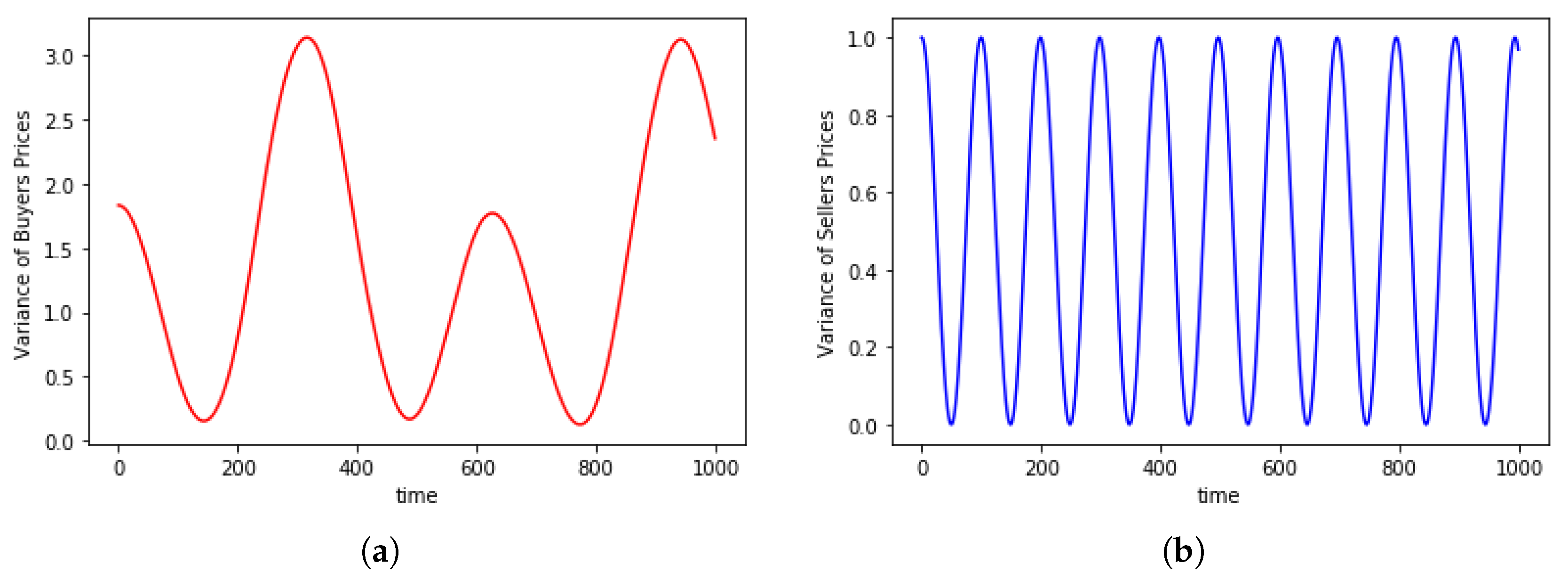
Figure 1 shows the temporal evolution of the system taking
, and
and
for a short term of
time steps. We can see that prices trend is made of regular waves maintaining same frequency and amplitude for each price, especially for the seller prices. The same behavior is observed in the price variances, both for buyers and sellers, as shown in
Figure 2.
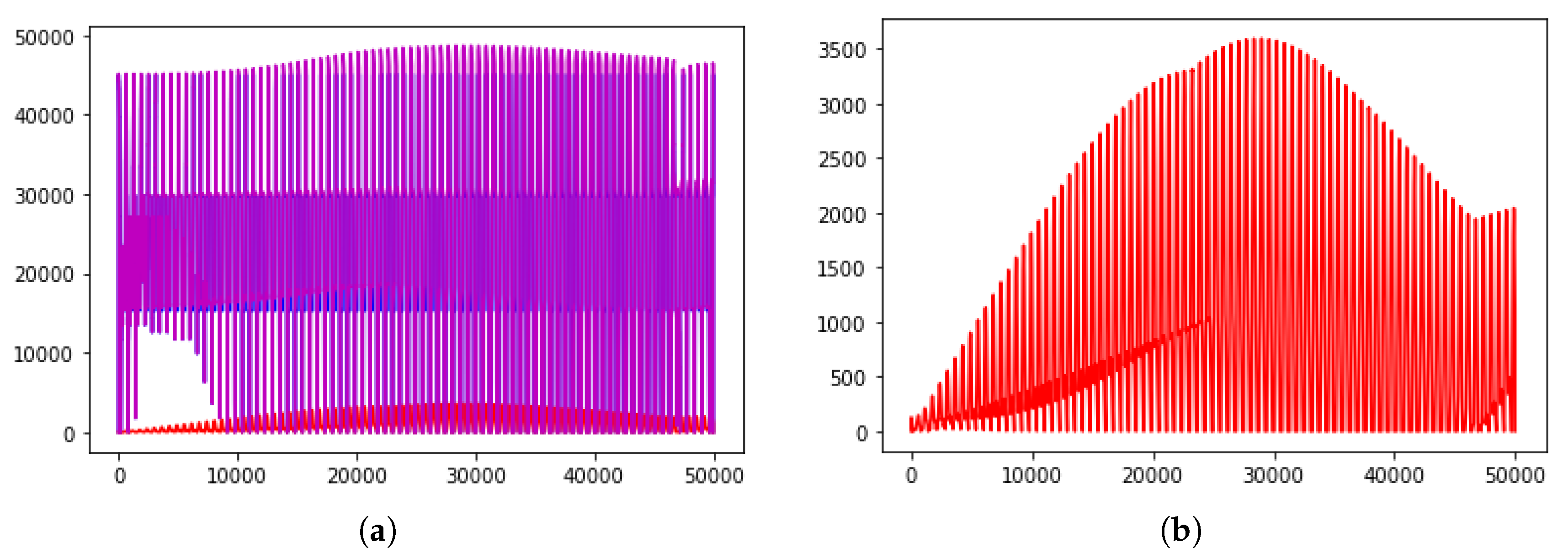
Figure 3 represents the corresponding Pareto market efficiencies for short and long terms, which are calculated as follows:
- -
Seller Pareto market efficiency is the sum, at every time t, of calculated at every exchange at a selling price and for every seller with initial cost , fixed from the beginning as of seller price.
- -
Buyer Pareto market efficiency is the sum, at every time t, of calculated at every exchange at a selling price and for every buyer with reservation price .
- -
The total Pareto market efficiency is the sum of the two above.
Notice that Pareto market efficiencies show a sort of regular and cyclical trend, where the benefits of the market are practically all on sellers, because of the sticking prices that were introduced for them and also for the choice made about the initial cost.
In addition, we aim to investigate the influence of some of the model parameters on the overall dynamics. For instance,
Figure 4 shows the trend for two values of
, namely
and
, while the other parameters keep the same value. Notice that there is a change in the ratio between the frequencies of the prices of the two different types of agents.
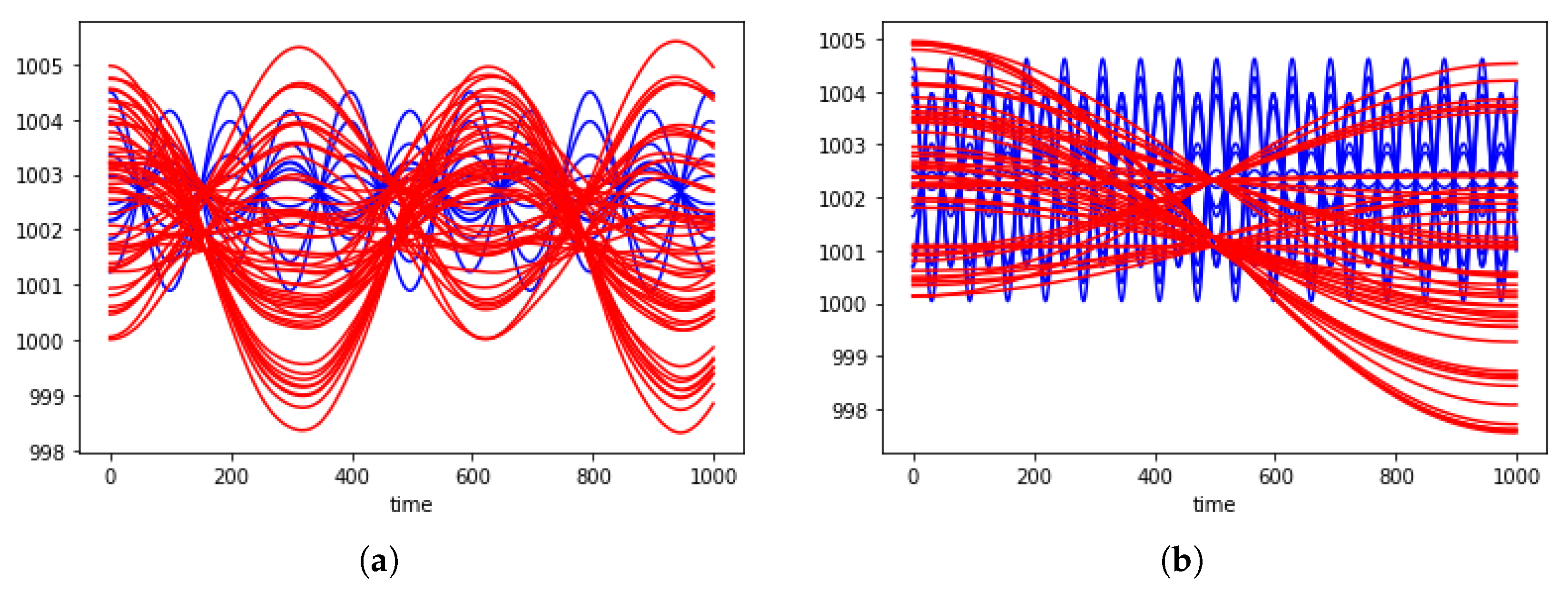
Both seller coordination and buyer differentiation in type are crucial. In particular, when we decrease seller coordination through
(which goes from
to
), buyer prices begin to change the amplitude of their waves during time and macro-waves appear in the long term, as shown in
Figure 5.
Taking a closer look to macro-waves, we can see that they are well differentiated depending on buyer type. That means that a lower seller coordination, brings both to the formation of clusters in the buyer functional subsystem, depending on their type, and to the aforementioned macro-waves. Recall that buyers
only seek the best quality, buyers
seek for the best quality-price ratio, while buyers
always choose the lowest price.
Figure 6 shows the dynamics for each type of buyer for different time intervals. In particular we use green for type
, purple for
and yellow for
. Although parameter
was reduced to
, all the other parameters keep the initially stated values. Three macro-waves emerge according to the type of buyer.
The stickiness of seller prices do not allow a visible change [for them] in their amplitude, as shown in
Figure 7.
However, even a small change in seller prices trend (which are more free to adapt to buyer ones due to a lower coordination) brings to an amplified effect on buyer prices, creating three different markets. Both the split and the macro-waves are a way for the buyer to reach (also creating it) the market they prefer. For example, macro-waves allow more often type
to have higher probability of grabbing the best quality. In this way, they also reach a higher Pareto market efficiency, as shown in
Figure 8. A similar result deriving from buyer coordination is also in [
23].
3.6. Numerical Results for Model 2
Recall that Model 2 assumes that each buyer has a reservation quality, which is the minimum level of quality that she/he is willing to accept for the product. Among those sellers satisfying the quality requirement, the buyer will choose the option with lowest price.
Consider the same initial conditions than in the previous case.
Figure 9 shows the dynamics for the short term of individual and mean prices.
As in the first case, when the value of
is changed, we can see macro-waves and a the formation of clusters depending on their (this time) reservation quality.
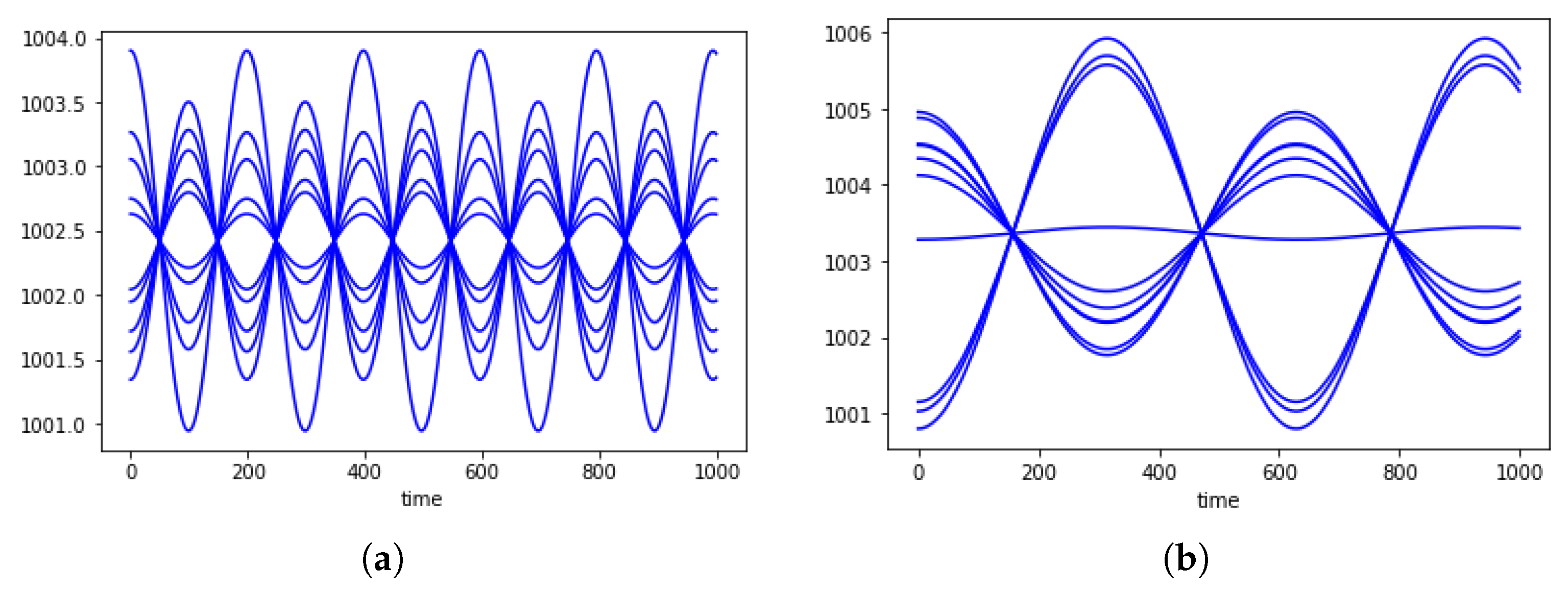
Figure 10 shows the case in which the 50 buyers are divided into six reservation qualities that, ordered from larger to lower, will be represented in black, red, cyan, yellow, green and magenta. It is clear that macro-waves emerge according to the reservation quality and this becomes especially clear for large times.
Notice that, as it usually happens in the simulations, in the short term (
Figure 10a) there are only three different trends for the six individuated groups, analogously to the first case (
Figure 6). But taking a look at the red and the black trends, if at the beginning (
Figure 10a) they stay together, in the medium term (
Figure 10c) we can see a slight differentiation in the frequency and, in the long term we can see that the red has got its own macrocycle (in
Figure 10d in the second half). Therefore, we end up with four different clusters
If the aforementioned trend is the most common, the split of the trends can also change depending on the (random) initial conditions of prices. Indeed, we can also see a fewer clusters and a unique cluster, as shown in
Figure 11. That means that the formation of clusters is an endogenous effect. In this sense, we may state that the second model is a generalization of the first one, in the sense that buyers can organize both in three clusters as in the first case, but also in more or less as it is more convenient for them.
4. Conclusions
In this paper, using [
2] as a base for our work, we developed the study of price dynamics, applying theory of swarms to describe the interactions of the particles living in our world. We introduced variables that can be seen as economic features. They are carried by particles that represent the agents divided in two different types: buyers and sellers. We showed a system in which the asymmetry between behaviors of the two types is a fundamental characteristic and a crucial aspect for the obtained results. We study the dynamics of prices in a perfect competitive market where also the parameter of quality is crucial. We used the idea of
cherry picking performed by buyers, which creates a more realistic behavior of our agents. In this context, the model explains the realistic behavior of markets besides the limits of the classical microeconomics models, with a unique price and a unique good; in the classical framework, goods with quality differences generate multiple markets. From that perspective, it is impossible to analyze the buyer behavior in the face of quality differences. Considering micro-transactions with prices exposed by the sellers (so-called adhesion contracts), we can instead investigate the effects of the consumer control about quality, e.g., in food and beverage markets, while cherry picking the products. The relevance of quality is related to goods with a limited range of prices. If the range is enormous, the quality usually is consistent with the price levels.
In
Section 2 we present the basis of our world, that will be completed in
Section 3. We set agent variables which are the price of the offered product for sellers and the reservation price for buyers. Price dynamics is based on the interaction (which affects the acceleration of prices) between two agents of the opposite type (
micro-micro interaction) and the interaction between an agent and the whole group it is part of (the
macro-micro interaction).
In
Section 3 we add the main characteristics of our model: the quality variable and
cherry picking (buyers choose seller to interact with, basing their choice on seller prices and qualities). We develop two models. In the first one we add quality as seller parameter and we distinguish three types of buyers on the different ways they choose sellers, every type basing its choice on different variables. In the second model we add also buyer reservation quality and every buyer chooses seller basing both on seller quality, with respect to its reservation one, and seller price. In this further development, the asymmetry consists of
cherry picking, in the
stickiness of sellers prices and in the idea that the buyer knows seller price and quality, but the seller does not know the buyer reservation price and quality (and this is reason it is the buyer to make the choice).
Computational results are also shown in
Section 3. If seller
macro-micro interaction is set sufficiently high, we obtain a regular oscillating trend for both seller and buyer prices. Wave trend has a length of few interactions and the amplitude remains always constant in time. Otherwise, if we lower the interaction among sellers, we see a more interesting behavior, which is the main result of our work. Seller prices do not seem to have an important change, while the buyer ones show a change in the amplitude of price waves during time that in the long term, creates macro-waves (with long wavelength). Moreover, every price follows a different macro-cycle depending on buyer type (for the first model) and buyer reservation quality (for second model). In this sense, the second case appear to be a generalization of the first one. We can explain this trend saying that a higher freedom for sellers, not bounded by the medium seller price, creates a little change in their prices, which brings to an acceleration in buyer ones. However, to understand better the economic reason behind this trend, we can see the effects on Pareto market efficiency, noticing that macro-waves are not only a way for buyer to “create” different markets to reach the best choice for their condition, but also a way to increase their own Pareto market efficiency. Our results also suggest a concrete consequence on reality, especially considering the increasing of markets where the competition and the number of relevant sellers are getting lower: when sellers create a sort of “agreement” about their prices (in the model, when they have a high interaction among them), buyers suffer of a drawback. On the other hand, a more free market means a gain for buyers, without a significant loss for sellers.


