Article

Pricing Various Types of Power Options under Stochastic Volatility

Department of Mathematics, Sogang University, Seoul 04107, Korea
*
Author to whom correspondence should be addressed.
Symmetry 2020, 12(11), 1911; https://doi.org/10.3390/sym12111911
Submission received: 21 October 2020 / Revised: 16 November 2020 / Accepted: 18 November 2020 / Published: 20 November 2020
(This article belongs to the Special Issue Advances in Stochastic Differential Equations)

Abstract

:
The exotic options with curved nonlinear payoffs have been traded in financial markets, which offer great flexibility to participants in the market. Among them, power options with the payoff depending on a certain power of the underlying asset price are widely used in markets in order to provide high leverage strategy. In pricing power options, the classical Black–Scholes model which assumes a constant volatility is simple and easy to handle, but it has a limit in reflecting movements of real financial markets. As the alternatives of constant volatility, we focus on the stochastic volatility, finding more exact prices for power options. In this paper, we use the stochastic volatility model introduced by Schöbel and Zhu to drive the closed-form expressions for the prices of various power options including soft strike options. We also show the sensitivity of power option prices under changes in the values of each parameter by calculating the resulting values obtained from the formulas.

1. Introduction

Power options are a class of exotic options in which the payoff at maturity is related to the certain positive power of the underlying asset price, which allows investors to a provide high leverage strategy and to hedge nonlinear price risks according to Tompkins [1]. Esser [2], Heynen and Kat [3], Tompkins [1], and Wilmott [4] are researches on the closed-form of the power option price under Black–Scholes [5] model.
While it is relatively easy to price power options based upon the classical Black–Scholes [5] model, there is the disadvantage of assuming a constant volatility which causes inevitable smiles or skews in the implied volatility of the underlying asset. For that account, it makes sense to consider a stochastic volatility model in valuing power options. Stochastic volatility models, such as Heston [6], Hull–White [7], Schöbel–Zhu [8], and Stein–Stein [9], are more popular and frequently used in the pricing of various kinds of European options. In spite of its effectiveness and importance, very little research has been done on pricing power options using stochastic volatility models mainly due to the sophisticated stochastic process for underlying assets, the more complex payoff structure and volatilities, and the difficulty of finding analytic forms of the option price.
To mention some of the works on pricing power options with stochastic volatilities, Bakshi and Madan [10] discuss a type of squared power payoffs in a general diffusion setup, but do not include detail calculations. Motivated by Scott [11], Kim et al. [12] derive semi-analytic forms for power option prices under the Heston model. Ibrahim et al. [13] derive the partial differential equation (PDE) from the Heston model for power option prices and solve the PDE for the characteristic function, and then apply the technique of fast Fourier transforms to price the power option under the Heston model.
In this paper, we use the stochastic volatility model introduced by Schöbel and Zhu [8] to drive a closed-form expression for the price of various power options. The Schöbel–Zhu model allows the volatility to follow an Ornstein–Uhlenbeck process which has a mean reversion property and is correlated with the return on asset. Esser [2] also derived semi-closed forms of the power option prices in the case of an Ornstein–Uhlenbeck process as a volatility process. One of the major advantages of using the Schöbel–Zhu model over the Heston model is the accessibility of the closed-form expression for the price of power options.
In Section 2, we first specify the dynamics of the processes of underlying asset and its volatility under the Schöbel–Zhu model, and then gain the pricing formula for a European power call option. Theorem 1 is the main result of the paper. In Section 3, using the results of the previous section, we drive the closed-form expressions for the prices of various types of power options and polynomial options. We also obtain the formula for the price of a soft strike option in the same section. In Section 4, we use the numerical computation to investigate the sensitivity of power option prices under changes in the values of each parameter in the Schöbel–Zhu model including the correlation between the two driving Brownian motions along with the change of the power α . Finally, we provide a conclusion and discussion in Section 5.

2. Model Specification and Pricing Formula for Power Options

For a dividend paying asset with the yield rate q, we assume the process of the asset price S t to have the following dynamics:
d S t = r q S t d t + v t S t d B t ,
d v t = κ θ v t d t + ξ d W t
under the risk-neutral probability measure Q , where B t and W t are two correlated standard Brownian motions with the correlation ρ , and r is the riskless rate. In addition, v t is the volatility of S t , which follows the Schöbel–Zhu [8] model process with constant parameters κ , θ , and ξ . The following two lemmas are about some special conditional expectation under the measure Q , all of which are important ingredients of the main result of the paper.
Lemma 1.
Under the assumptions of (1) and (2) with α > 0 , we get the following equality:
E Q S T α F t = S t α e α r q T t ρ α 2 ξ v t 2 + ξ 2 T t E Q e t T c 1 v s 2 + c 2 v s d s + c 3 v T 2 F t ,
where c 1 , c 2 and c 3 are constants with:
c 1 = α 1 α 1 ρ 2 2 ρ κ ξ , c 2 = ρ α κ θ ξ , c 3 = ρ α 2 ξ .
Proof. 
From (1), we get:
E Q S T α F t = S t α e α r q T t E Q e α 2 α 1 ρ 2 1 t T v s 2 d s + ρ α t T v s d W s F t
by writing B t = ρ W t + 1 ρ 2 W ^ t with W ^ t as a Q -standard Brownian motion independent of W t and using the tower property. Applying the Itô formula to v t 2 , we have:
d v t 2 = 2 κ ξ 2 2 κ + θ v t v t 2 d t + 2 ξ v t d W t ,
which implies that:
t T v s d W s = 1 2 ξ v T 2 v t 2 ξ 2 T t 2 κ θ t T v s d s + 2 κ t T v s 2 d s .
Substituting (4) into (3), we obtain:
E Q S T α F t = S t α e α r q T t ρ α 2 ξ v t 2 + ξ 2 T t E Q e t T c 1 v s 2 + c 2 v s d s + c 3 v T 2 F t
with
c 1 = α 1 α 1 ρ 2 2 ρ κ ξ , c 2 = ρ α κ θ ξ , c 3 = ρ α 2 ξ .
 □
Now, we need the following result of Schöbel and Zhu [8] to get the detailed value of E Q S T α F t mentioned above.
Lemma 2.
Under the assumption of (2), together with constants c 1 , c 2 , and c 3 , we get the following equality:
E Q e t T c 1 v s 2 + c 2 v s d s + c 3 v T 2 F t = A t e B t v t 2 + C t v t ,
where
A t = 1 Ψ γ 1 , γ 2 × exp κ T t 2 + κ 2 θ 2 γ 1 2 γ 3 2 2 ξ 2 γ 1 3 sinh γ 1 T t Ψ γ 1 , γ 2 γ 1 T t + κ θ γ 1 γ 2 γ 3 γ 3 ξ 2 γ 1 3 cosh γ 1 T t 1 Ψ γ 1 , γ 2 ,
B t = 1 2 ξ 2 κ γ 1 Φ γ 1 , γ 2 Ψ γ 1 , γ 2
and
C t = 1 ξ 2 γ 1 κ θ γ 1 γ 2 γ 3 + γ 3 Φ γ 1 , γ 2 Ψ γ 1 , γ 2 κ θ γ 1
with
Φ γ 1 , γ 2 = sinh γ 1 T t + γ 2 cosh γ 1 T t , Ψ γ 1 , γ 2 = cosh γ 1 T t + γ 2 sinh γ 1 T t
and
γ 1 = κ 2 + 2 c 1 ξ 2 , γ 2 = κ 2 c 3 ξ 2 γ 1 , γ 3 = κ 2 θ c 2 ξ 2 .
Proof. 
The proof appears in the appendix of [8]. □
Using Lemma 1 and Lemma 2, we can get a closed-form expression of the price of a European power- α call option with strike price K whose payoff at maturity T is given by max S T α K , 0 .
Theorem 1.
Let us denote the log-asset price by x t = ln S t α . Under the assumptions of (1) and (2), the price of a European power-α call option with strike price K and maturity T is given by:
C t , S t α = E Q S T α F t e r T t P 1 K e r T t P 2 ,
where P 1 , P 2 are defined by:
P j = 1 2 + 1 π 0 Re e i ϕ ln K f j ϕ i ϕ d ϕ
for j = 1 , 2 , in which:
f 1 ϕ = e 1 + i ϕ α r q ρ ξ 2 T t + x t ρ α 2 ξ v t 2 E Q S T α F t E Q e t T m 1 v s 2 + m 2 v s d s + m 3 v T 2 F t
with
m 1 = α 1 + i ϕ 1 α 1 ρ 2 2 ρ κ ξ , m 2 = ρ α κ θ ξ 1 + i ϕ , m 3 = ρ α 2 ξ 1 + i ϕ
and
f 2 ϕ = e i ϕ α r q ρ ξ 2 T t + x t ρ α 2 ξ v t 2 E Q S T α F t E Q e t T n 1 v s 2 + n 2 v s d s + n 3 v T 2 F t
with
n 1 = i α ϕ 1 α 1 ρ 2 2 ρ κ ξ , n 2 = i ρ α κ θ ϕ ξ , n 3 = i ρ α ϕ 2 ξ .
Proof. 
From the risk-neutral valuation, the price of a European power- α call option with strike price K and maturity T is given by:
C t , S t α = e r T t E Q max S T α K , 0 F t = e r T t E Q S T α K 𝟙 S T α > K F t = e r T t E Q S T α 𝟙 S T α > K F t K e r T t E Q 𝟙 S T α > K F t .
For a new risk-neutral probability measure Q ˜ , the Radon–Nikodým derivative of Q ˜ with respect to Q is defined by:
d Q ˜ d Q = S T α E Q S T α F t
on F t . Then the price can be rewritten as:
C t , S t α = e r T t E Q S T α F t Q ˜ S T α > K K e r T t Q S T α > K = e r T t E Q S T α F t P 1 K e r T t P 2
with the risk-neutralized probabilities P 1 and P 2 . Now, putting x t = ln S t α , the corresponding characteristic functions f 1 and f 2 can be represented as:
f 1 ϕ = E Q ˜ e i ϕ x T F t = 1 E Q S T α F t E Q e 1 + i ϕ x T F t , f 2 ϕ = E Q e i ϕ x T F t .
On the other hand, applying the Itô formula to (1), we have:
d x t = α r q 1 2 v t 2 d t + ρ α v t d W t + α 1 ρ 2 v t d W ^ t .
From Lemma 1, we obtain:
f 1 ϕ = e 1 + i ϕ α r q ρ ξ 2 T t + x t ρ α 2 ξ v t 2 E Q S T α F t E Q e t T m 1 v s 2 + m 2 v s d s + m 3 v T 2 F t
with
m 1 = α 1 + i ϕ 1 α 1 ρ 2 2 ρ κ ξ , m 2 = ρ α κ θ ξ 1 + i ϕ , m 3 = ρ α 2 ξ 1 + i ϕ .
Similarly, we also obtain:
f 2 ϕ = e i ϕ α r q ρ ξ 2 T t + x t ρ α 2 ξ v t 2 E Q S T α F t E Q e t T n 1 v s 2 + n 2 v s d s + n 3 v T 2 F t
with
n 1 = i α ϕ 1 α 1 ρ 2 2 ρ κ ξ , n 2 = i ρ α κ θ ϕ ξ , n 3 = i ρ α ϕ 2 ξ .
Here, each value of the above risk-neutral expectation was obtained in previous lemmas.
By obtaining closed-form expressions for the characteristic functions f 1 and f 2 , the Fourier inversion formula allows us to compute the probabilities P 1 and P 2 as follows:
P j = 1 2 + 1 π 0 Re e i ϕ ln K f j ϕ i ϕ d ϕ
for j = 1 , 2 . □

3. Application to Various Power Payoffs

In general, there are two kinds of power options since the power can be applied either to the underlying asset price at maturity or to the entire vanilla option payoff. We call those options asymmetric and symmetric power options, respectively. In Theorem 1, we have derived the pricing formula for asymmetric power options. The pricing formula for symmetric power options is more complicated. Still, symmetric power options are preferred by some users as their return patterns are different from those of asymmetric ones with the same power parameters. Here, we only focus on the case of a positive integer power.

3.1. Symmetric Power Option

For a positive integer n and the central strike price K, the payoff of a European symmetric power-n call option at maturity T is given by:
max S T K , 0 n = S T K n 𝟙 S T > K = j = 0 n n j S T n j K j 𝟙 S T > K ,
where n j = n ! j ! n j ! .
Since the option price is given by:
C t , S t n = e r T t E Q max S T K , 0 n F t ,
where
E Q max S T K , 0 n F t = E Q j = 0 n n j S T n j K j 𝟙 S T > K F t = j = 0 n n j K j E Q S T n j 𝟙 S T > K F t ,
we need the calculation of E Q S T n j 𝟙 S T > K F t .
As before, the Radon–Nikodým derivative of the new risk-neutral probability measure Q ˜ with respect to Q is defined by:
d Q ˜ d Q = S T n j E Q S T n j F t
on F t . Then we have:
E Q S T n j 𝟙 S T > K F t = E Q S T n j F t Q ˜ S T > K .
Here, we can compute E Q S T n j F t by substituting n j instead of α obtained the result in Lemma 1. Furthermore, putting y t = ln S t , the corresponding characteristic function f can be represented as:
f ϕ = E Q ˜ e i ϕ y T F t = 1 E Q S T n j F t E Q e n j + i ϕ y T F t .
On the other hand, applying the Itô formula to (1), we have:
d y t = r q 1 2 v t 2 d t + ρ v t d W t + 1 ρ 2 v t d W ^ t .
From Lemma 1, we obtain:
f ϕ = e n j + i ϕ r q ρ ξ 2 T t + y t ρ 2 ξ v t 2 E Q S T n j F t E Q e t T u 1 v s 2 + u 2 v s d s + u 3 v T 2 F t
with
u 1 = ρ n j + i ϕ ρ 2 κ ξ , u 2 = ρ κ θ ξ n j + i ϕ , u 3 = ρ 2 ξ n j + i ϕ .
Here, each value of the above risk-neutral expectation was also obtained in previous lemmas.
By also obtaining the closed-form expression for the characteristic function f, the Fourier inversion formula allows us to compute the risk-neutral probability P : = Q ˜ S T > K as follows:
P = 1 2 + 1 π 0 Re e i ϕ ln K f ϕ i ϕ d ϕ .

3.2. Polynomial Options

A polynomial call option is a European call whose payoff represents the difference between a polynomial expression of the asset price at maturity and the strike price. As explained in [14], a polynomial option can be decomposed as a sum of power options. To get the price of a polynomial option, we need to find the roots of the characteristic polynomial function associated to the payoff function.
Here, we focus on the type of a polynomial call option mentioned in [14]. Let A x = j = 1 n a j x j be the polynomial function with degree n and coefficients a j ’s, and let K be the positive real number such that the polynomial function A x K has exactly p strictly positive roots λ 1 , λ 2 , , λ p with λ 1 < λ 2 < < λ p , and A x K alternates its sign between two consecutive roots with A x K for 0 x λ 1 . Then the payoff is given by:
max A S T K , 0 .
Thus, we have:
E Q max A S T K , 0 F t = E Q j = 1 n a j k = 1 p 1 k + 1 C j λ k j , T F t = k = 1 p j = 1 n a j 1 k + 1 E Q C j λ k j , T F t = k = 1 p j = 1 n a j 1 k + 1 E Q max S T j λ k j , 0 F t ,
where C j λ , T represents the price of a European power-j call option with the strike price λ at maturity T.

3.3. Soft Strike Options

For the central strike price K and ω 0 , K , the payoff of the soft strike call option C ω ( S T ) is given by:
C ω ( S T ) = 0 if S T < K ω , 1 4 ω S T K + ω 2 if K ω S T K + ω , S T K if S T > K + ω .
Then we can see that C ω ( S T ) max S T K , 0 as ω 0 . In contrast to the standard call payoff max S T K , 0 , C ω ( S T ) has a continuous derivative C ω ( S T ) given by:
C ω ( S T ) = 0 if S T < K ω , 1 2 ω S T K + ω if K ω S T K + ω , 1 if S T > K + ω
for all S T and a piecewise constant second derivative. Since Gamma ( Γ ) is the second differential of the derivative price with respect to the asset price, it is therefore constant for a soft strike options near its maturity. In contrast, the standard call payoff where Gamma ( Γ ) blows up when the asset price is close to the strike price has high risks associated with hedging the option which is close to its maturity. We can see more details on soft strike options in [1,15].
To evaluate the price of a soft strike option, we have to calculate that:
E Q 1 4 ω S T K + ω 2 𝟙 K ω S T K + ω F t + E Q S T K 𝟙 S T > K + ω F t = 1 4 ω E Q S T 2 𝟙 K ω S T K + ω F t 2 K ω E Q S T 𝟙 K ω S T K + ω F t + K ω 2 E Q 𝟙 K ω S T K + ω F t + E Q S T 𝟙 S T > K + ω F t K E Q 𝟙 S T > K + ω F t .
Note that in the first term of the equality:
E Q S T 2 𝟙 K ω S T K + ω F t = E Q S T 2 𝟙 S T K ω F t E Q S T 2 𝟙 S T > K + ω F t = E Q S T 2 F t Q ˜ S T K ω Q ˜ S T > K + ω
as in (5) by substituting 2 for n j . Note also that in the second term of the equality:
E Q S T 𝟙 K ω S T K + ω F t = E Q S T 𝟙 S T K ω F t E Q S T 𝟙 S T > K + ω F t = E Q S T F t Q ˜ S T K ω Q ˜ S T > K + ω
as in (5) by substituting 1 for n j . Likewise, we can obtain the value of E Q S T 𝟙 S T > K + ω F t in the fourth term of the equality. Moreover, we have:
E Q 𝟙 K ω S T K + ω F t = Q S T K ω Q S T > K + ω
and
E Q 𝟙 S T > K + ω F t = Q S T > K + ω ,
which are the values obtained by substituting 1 for n from f 2 ϕ in Theorem 1.

4. Numerical Experiments

In this section, with the numerical computation, we investigate the sensitivity of the power option prices under the changes in the values of each parameter in the Schöbel–Zhu model along with the increase of the power α . We use the Scipy package and Sdeint package in Python.

4.1. The General Case

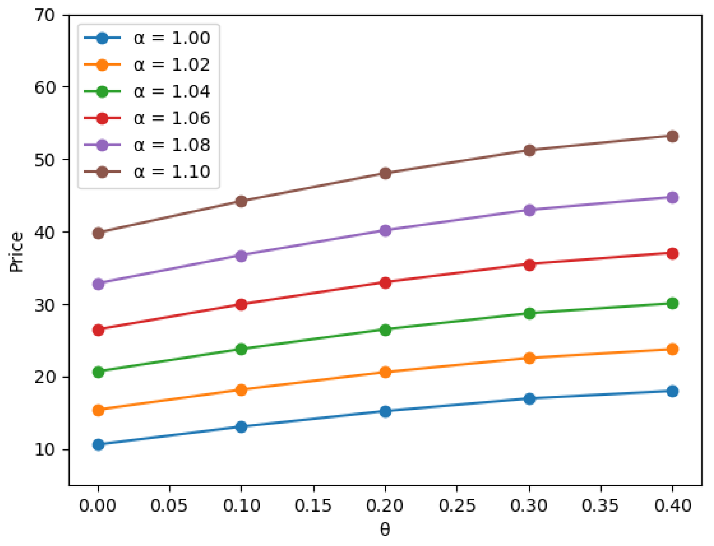
The parameter ρ is the correlation between two standard Brownian motions B t and W t , θ is the mean long-term variance, κ is the rate at which the variance reverts toward its long-term mean, and ξ is the volatility of the variance process in the Schöbel–Zhu model. By assuming that S = 100 , K = 80 , T t = 0.5 , r = 0.05 , and q = 0.02 for each calculation of formula given in Theorem 1, we observe the change of power option prices as we switch the values of each parameter and the power α . In each case, as α is increasing the option price is getting higher as expected. In addition, for different α , the pattern of option price change is very similar and stable as we switch the value of κ , θ , ξ , and ρ , respectively.
Table 1 and Figure 1 demonstrate the change of power option prices as we switch the values of κ and α . For each fixed α , the option prices are almost unchanged with different values of κ .
Table 2 and Figure 2 show the change of power option prices as we switch the values of θ and α . For each fixed α , the option price is increasing with the similar pattern as for the other fixed α case, when θ is increasing.
Table 3 and Figure 3 show the change of power option prices as we switch the values of ξ and α . For each fixed α , the option price is decreasing with a similar pattern when ξ is increasing.
Table 4 and Figure 4 show the change of power option prices as we switch the values of ρ and α , which may be of special interest since the statistical dependence between the underlying asset and its volatility may have a substantial impact in the price of contingent claims. For each fixed α , the option price is decreasing with a similar pattern as for the other fixed α case, when ρ is increasing.

4.2. The Symmetric Case

Similarly, we compute the symmetric power option prices for n = 2 in the same way to previous subsection. Table 5, Table 6, Table 7 and Table 8 show the relationship between the symmetric power option price and parameters. The option prices move to the same direction as the general power option prices with the increase of θ , ξ , and ρ . On the other hand, the option price changes rapidly with respect to the increase of each parameter.

5. Conclusions and Discussion

In this paper, we drive a closed-form expression for the price of power options by using the Schöbel–Zhu stochastic volatility model whose volatility, correlated with the return on asset, follows an Ornstein–Uhlenbeck process with a mean reversion property. Then, with the numerical computation, we investigate the sensitivity of power option prices under changes in the values of each parameter along with the increase of power α from 1.00 to 1.10 . Since our pricing formula is available in closed form, it is theoretically possible to differentiate the price formula with respect to each parameter to obtain sensitivity expressions in closed form. Finding that obtaining such derivatives is rather complicated work, we used the Python package to compute and observe the relationship between the power option price and each parameter including α . We see that, for different α , the pattern of option price change was very similar and stable enough to perform analysis in real market as the value of κ , θ , ξ , and ρ , was respectively switched.
Since the statistical dependence between the underlying asset and its volatility may have a substantial impact in the power option price, one may expect our assumption of constant correlation between two standard Brownian motions could be improved. However, applying stochastic correlations between two standard Brownian motions in our cases could make it much harder to get the closed-form expressions for the prices of power options while gaining not as much advantage of overcoming correlation risks. Since correlation plays an important role in pricing multi-asset options, we would like to incorporate stochastic correlations into pricing power quanto options, which will be our next research project.
For the case of symmetric power options, since we used the polynomial expansion, the smallest power we could use is n = 2 which is substantially bigger than previously used α so that the option price is much more sensitive with respect to the increase of each parameter. We leave the issue of pricing symmetric power options with the power 1 < α < 2 using the Schöbel–Zhu stochastic volatility model to future work.

Author Contributions

Conceptualization, J.L. and Y.L.; methodology, Y.L.; formal analysis, Y.L.; software, Y.K.; visualization, Y.K.; validation, Y.L. and Y.K.; writing—original draft preparation, J.L. and Y.L.; writing—review and editing, J.L., Y.L. and Y.K.; supervision, J.L. All authors have read and agreed to the published version of the manuscript.

Funding

This research received no external funding.

Acknowledgments

The authors want to express their heartfelt appreciation to the anonymous referee and the editor for their important comments, which were significantly helpful for the authors’ further research.

Conflicts of Interest

The authors declare no conflict of interest.

References

  1. Tompkins, R.G. Power options: Hedging nonlinear risks. J. Risk 1999, 2, 29–45. [Google Scholar] [CrossRef]
  2. Esser, A. General variation Principles for Arbitrary payoffs and applications to power options under stochastic volatility. Financ. Mark. Portf. Manag. 2003, 17, 351–372. [Google Scholar] [CrossRef]
  3. Heynen, R.C.; Kat, H.M. Pricing and hedging power options. Financ. Eng. Jpn. Mark. 1996, 3, 253–261. [Google Scholar] [CrossRef]
  4. Wilmott, P. Derivatives: The Theory and Practice of Financial Engineering; Wiley: New York, NY, USA, 1998. [Google Scholar]
  5. Black, F.; Scholes, M. The pricing of options and corporate liabilities. J. Political Econ. 1973, 81, 637–654. [Google Scholar] [CrossRef] [Green Version]
  6. Heston, S.L. A closed-form solution for options with stochastic volatility with applications to bond and currency options. Rev. Financ. Stud. 1993, 6, 327–343. [Google Scholar] [CrossRef] [Green Version]
  7. Hull, J.; White, A. The pricing of options on assets with stochastic volatilities. J. Financ. 1987, 42, 281–300. [Google Scholar] [CrossRef]
  8. Schöbel, R.; Zhu, J. Stochastic volatility with an Ornstein-Uhlenbeck process: An extension. Eur. Financ. Rev. 1999, 3, 23–46. [Google Scholar] [CrossRef]
  9. Stein, E.M.; Stein, J.C. Stock price distributions with stochastic volatility: An analytic approach. Rev. Financ. Stud. 1991, 4, 727–752. [Google Scholar] [CrossRef]
  10. Bakshi, G.; Madan, D. Spanning and derivative-security valuation. J. Financ. Econ. 2000, 55, 205–238. [Google Scholar] [CrossRef]
  11. Scott, L. Pricing stock options in a jump-diffusion model with stochastic volatility and interest rates: Applications of Fourier inversion methods. Math. Financ. 1997, 7, 413–424. [Google Scholar] [CrossRef]
  12. Kim, J.; Kim, B.; Moon, K.-S.; Wee, I.-S. Valuation of power options under Heston’s stochastic volatility model. J. Econ. Dyn. Control 2012, 36, 1796–1813. [Google Scholar] [CrossRef]
  13. Ibrahim, S.N.I.; O’Hara, J.G.; Constantinou, N. Pricing power options under the Heston dynamics using the FFT. New Trends Math. Sci. 2013, 1, 1–9. [Google Scholar]
  14. Macovschi, S.; Quittard-Pinon, F. On the pricing of power and other polynomial options. J. Deriv. 2006, 13, 61–71. [Google Scholar] [CrossRef]
  15. Hart, I.; Ross, M. Striking continuity. Risk 1994, 7, 51–56. [Google Scholar]
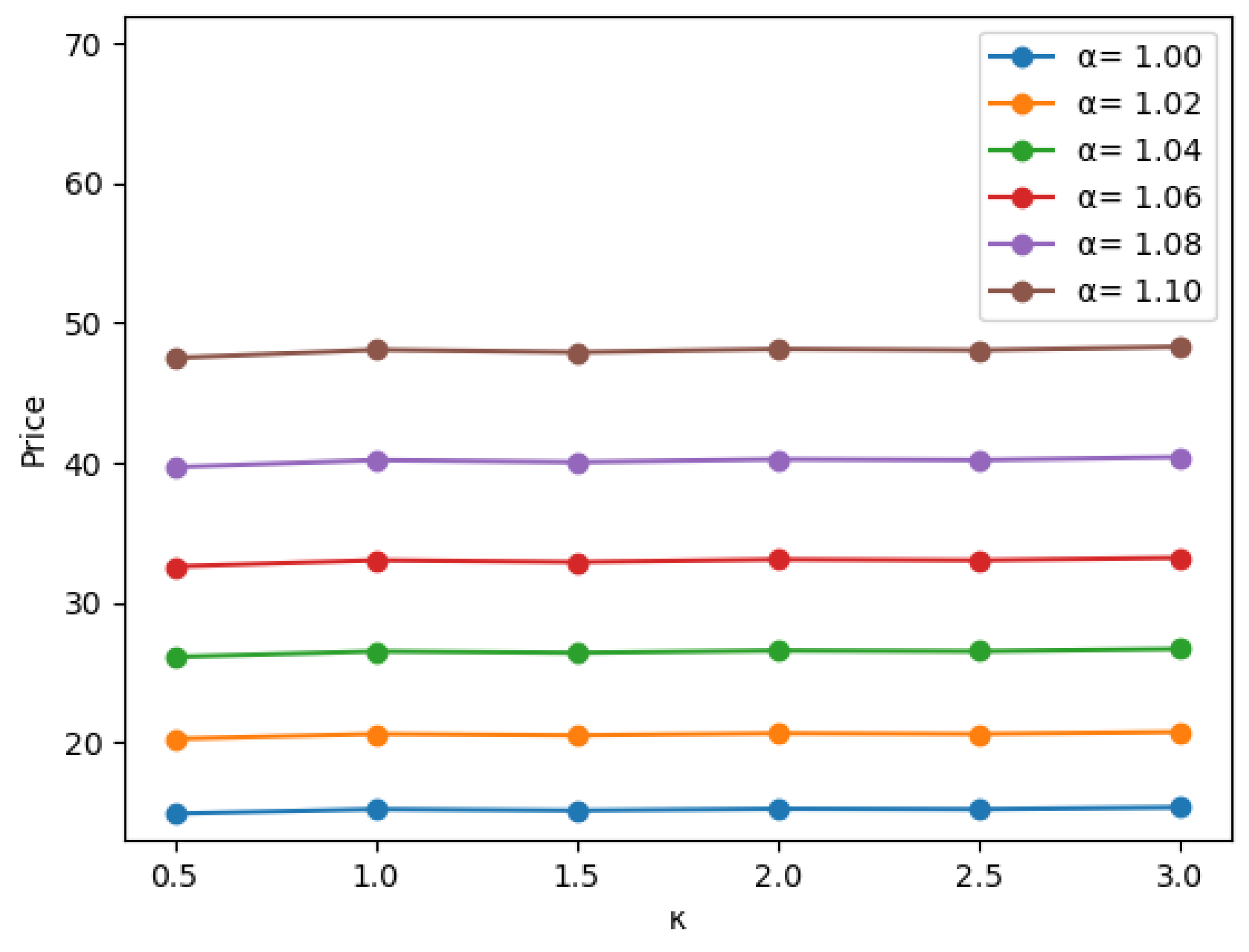
Figure 1. The relation between κ and prices.
Symmetry 12 01911 g001
Figure 2. The relation between θ and prices.
Symmetry 12 01911 g002
Figure 3. The relation between ξ and prices.
Symmetry 12 01911 g003
Figure 4. The relation between ρ and prices.
Symmetry 12 01911 g004
Table 1. The relation between κ and prices. S = 100 , K = 80 , T t = 0.5 , r = 0.05 , q = 0.02 , θ = 0.2 , ξ = 0.4 , and ρ = 0.5 .
α 1.00 1.02 1.04 1.06 1.08 1.10
κ
0.5 14.9602 20.2509 26.1164 32.5757 39.6907 47.4996
1.0 15.2305 20.6047 26.5185 32.0335 40.1910 48.0786
1.5 15.1380 20.5057 26.4116 32.9027 40.0499 47.9059
2.0 15.2287 20.6531 26.5154 32.0269 40.1845 48.0589
2.5 15.2286 20.6070 26.5239 32.0315 40.1913 48.0525
3.0 15.3656 20.7493 26.6874 32.2116 40.4029 48.2944
Table 2. The relation between θ and prices. S = 100 , K = 80 , T t = 0.5 , r = 0.05 , q = 0.02 , κ = 2 , ξ = 0.4 , and ρ = 0.5 .
α 1.00 1.02 1.04 1.06 1.08 1.10
θ
0.0 10.6090 15.4146 20.6931 26.4904 32.8560 39.8447
0.1 13.0813 18.1847 23.7941 29.9698 36.7552 44.2054
0.2 15.2287 20.6031 26.5154 33.0269 40.1845 48.0589
0.3 16.9669 22.5634 28.7321 35.5366 42.9980 51.2359
0.4 18.0210 23.7736 30.1102 37.0876 44.7763 53.2598
Table 3. The relation between ξ and prices. S = 100 , K = 80 , T t = 0.5 , r = 0.05 , q = 0.02 , κ = 2 , θ = 0.2 , and ρ = 0.5 .
α 1.00 1.02 1.04 1.06 1.08 1.10
ξ
0.1 33.3792 41.0389 49.4924 58.8494 69.1927 80.6479
0.2 20.6700 26.7056 33.3712 40.7167 48.8059 57.7199
0.3 16.9545 22.5310 28.6808 35.4542 42.8946 51.0943
0.4 15.2287 20.6031 26.5154 33.0269 40.1845 48.0589
0.5 14.2011 19.4552 25.2250 31.5801 38.5712 46.2667
Table 4. The relation between ρ and prices. S = 100 , K = 80 , T t = 0.5 , r = 0.05 , q = 0.02 , κ = 2 , θ = 0.2 , and ξ = 0.4 .
α 1.00 1.02 1.04 1.06 1.08 1.10
ρ
1.00 20.6539 26.7006 33.3639 40.7141 48.8088 57.7294
0.75 17.8747 23.5758 29.8529 36.7716 44.3839 52.7656
0.50 15.2287 20.6031 26.5154 33.0269 40.1845 48.0589
0.25 12.7100 17.7755 23.3432 29.4704 36.1996 43.5962
0.00 10.3129 15.0862 20.3285 26.0932 32.4186 39.3655
0.25 8.0320 12.5291 17.4640 22.8867 28.8315 35.3550
0.50 5.8622 10.0981 14.7427 19.8428 25.4289 31.5538
0.75 3.7989 7.7878 12.1582 16.9537 22.2018 27.9514
1.00 1.8374 5.5927 9.7040 14.2123 19.1418 24.5381
Table 5. The relation between κ and prices when n = 2 . S = 100 , K = 80 , T t = 0.5 , r = 0.05 , q = 0.02 , θ = 0.4 , ξ = 0.14 , and ρ = 0.52 .
κ 2.00 2.25 2.50 2.75 3.00
Prices 41.8056 59.1852 83.1452 95.6851 107.2798
Table 6. The relation between θ and prices when n = 2 . S = 100 , K = 80 , T t = 0.5 , r = 0.05 , q = 0.02 , κ = 2 , ξ = 0.14 , and ρ = 0.53 .
θ 0.40 0.41 0.42 0.43 0.44
Prices 147.1643 218.7923 286.2040 343.9156 399.0800
Table 7. The relation between ξ and prices when n = 2 . S = 100 , K = 80 , T t = 0.5 , r = 0.05 , q = 0.02 , κ = 2 , θ = 0.4 , and ρ = 0.52 .
ξ 0.130 0.132 0.134 0.136 0.138 0.140
Prices 469.1018 365.7494 282.3005 206.7740 124.4067 41.8056
Table 8. The relation between ρ and prices when n = 2 . S = 100 , K = 80 , T t = 0.5 , r = 0.05 , q = 0.02 , κ = 2 , θ = 0.4 , and ξ = 0.14 .
ρ 0.550 0.545 0.540 0.535 0.530 0.525 0.520
Prices 378.1934 319.2700 261.1295 203.7638 147.1643 91.3230 41.8056
Publisher’s Note: MDPI stays neutral with regard to jurisdictional claims in published maps and institutional affiliations.