A Novel Numerical Algorithm to Estimate the Subdivision Depth of Binary Subdivision Schemes

Abstract

Subdivision schemes are extensively used in scientific and practical applications to produce continuous geometrical shapes in an iterative manner. We construct a numerical algorithm to estimate subdivision depth between the limit curves/surfaces and their control polygons after k-fold subdivisions. In this paper, the proposed numerical algorithm for subdivision depths of binary subdivision curves and surfaces are obtained after some modification of the results given by Mustafa et al in 2006. This algorithm is very useful for implementation of the parametrization.

1. Introduction

Computer Aided Geometric Design (CAGD) foremost deals with curves/surfaces and its computational aspects. Subdivision schemes (SSs) have achieved much popularity in the past few years because of its competitive generation of curves/surfaces, and this magnificence lies in its implementation along with its mathematical formulation. Here we provide an overview of CAGD, subdivision and some other related concepts. The term CAGD was first suggested by Riesenfeld and Barnhill [1] in 1974 and the initial work was performed in the 1960’s. “Computational Geometry for Design and Manufacture” was the first book on CAGD authored by Faux and Pratt [2] in 1979. Subdivision is the most remarkable field for the purpose of modeling in CAGD, and is described as “the act or process of dividing something into smaller parts”. A small number of papers have been published in the field of SSs for error dominance.

Huawei et al. [3] performed error (distance) estimations for the Doo–Sabin scheme. After this, Mustafa et al. [4,5,6,7] estimated error bounds for binary, non-stationary binary, ternary and quaternary SSs. Mustafa et al. computed error bounds for tensor product volumetric models and $\sqrt{3}$ subdivision surfaces [8,9]. They also computed triangular surfaces subdivision depths [10]. However, Mustafa and Hashmi [11] determined subdivision depth computation for n-ary subdivision curves/surfaces by using the first forward difference technique. Moncayo and Amat [12] estimated error bounds for the class of SSs based on the two-scale refinement equation. The authors in [4,5,6,7,8,9,10,11] imposed these conditions to find their results. But, it has been observed that all SSs do not satisfy the imposed condition. Amat et al. [12] relaxed the condition in [4] for estimating the error bounds of binary SSs for curve designing. In this paper, we relax the conditions in the work of [5,6,7,8,9,10,11] and generalize the work of [12] to estimating error bounds and subdivision depths of binary SSs for curve and regular surface design.

However, as of yet, no one has found a numerical algorithm to estimate error bounds and subdivision depths of parametric SSs for curve and regular surface design. This motivates us to present a novel numerical algorithm for estimating the subdivision depth of binary subdivision schemes. This paper introduces not only a numerical algorithm for parametric SSs, but also the estimation for the non-parametric SSs. This novel technique has lesser computational cost than numerous other techniques.

Now we present some preliminaries. In the case of the curve: Let $\{f_i^k;i\in \mathbf{Z}\}$ be a sequence of points in ${\mathbf{R}}^{\mathbf{N}}$, where $\mathbf{N}\ge 2$ and k be the non-negative integer which indicates the SS level. A generalized univariate binary SS [13] is illustrated in the following as

$$\left\{\begin{array}{c}{f}_{2i}^{k+1}={\displaystyle \sum _{m=0}^t}{a}_{0,m}{f}_{i+m}^k,\hfill \\ f_{2i+1}^{k+1}={\displaystyle \sum _{m=0}^t}{a}_{1,m}{f}_{i+m}^k,\hfill \end{array}\right.$$

(1)

with necessary condition of the convergence

$$\begin{array}{c}\hfill {\displaystyle \sum _{m=0}^t}{a}_{0,m}={\displaystyle \sum _{m=0}^t}{a}_{1,m}=1.\end{array}$$

(2)

By [4], we have

$$\begin{array}{ccc}\hfill b_{0,m}& =& {\displaystyle \sum _{l=0}^m}\left(a_{0,l}-a_{1,l}\right),\hfill \\ \hfill b_{1,m}& =& a_{0,m}-b_{0,m},\hfill \end{array}$$

(3)

such that

$${\displaystyle \sum _{m=0}^t}|b_{0,m}|<1\mathrm{and}{\displaystyle \sum _{m=0}^t}|b_{1,m}|<1.$$

We introduce the coefficients for $m=0,1,\dots ,t$, such that

$$\begin{array}{c}\hfill \left\{\begin{array}{c}{d}_{2m}=b_{0,m},\hfill \\ d_{2m+1}=b_{1,m}.\hfill \end{array}\right.\end{array}$$

(4)

In the case of the surface: The points $\{f_{i,j}^k;i,j\in \mathbf{Z}\}$ represents a sequence in ${\mathbf{R}}^{\mathbf{N}}$, $\mathbf{N}\ge 2$ and is described as

$$\begin{array}{c}\hfill \left\{\begin{array}{c}{f}_{2i,2j}^{k+1}={\displaystyle \sum _{p=0}^t}{\displaystyle \sum _{q=0}^t}{a}_{0,p}{a}_{0,q}{f}_{i+p,j+q}^k,\hfill \\ f_{2i,2j+1}^{k+1}={\displaystyle \sum _{p=0}^t}{\displaystyle \sum _{q=0}^t}{a}_{0,p}{a}_{1,q}{f}_{i+p,j+q}^k,\hfill \\ f_{2i+1,2j}^{k+1}={\displaystyle \sum _{p=0}^t}{\displaystyle \sum _{q=0}^t}{a}_{1,p}{a}_{0,q}{f}_{i+p,j+q}^k,\hfill \\ f_{2i+1,2j+1}^{k+1}={\displaystyle \sum _{p=0}^t}{\displaystyle \sum _{q=0}^t}{a}_{1,p}{a}_{1,q}{f}_{i+p,j+q}^k,\hfill \end{array}\right.\end{array}$$

(5)

with the condition

$$\begin{array}{c}\hfill {\displaystyle \sum _{p=0}^t}{a}_{0,p}={\displaystyle \sum _{p=0}^t}{a}_{1,p}={\displaystyle \sum _{q=0}^t}{a}_{0,q}={\displaystyle \sum _{q=0}^t}{a}_{1,q}=1.\end{array}$$

(6)

By [4], we have

$${\displaystyle \sum _{p=0}^t}|a_{0,p}|{\displaystyle \sum _{q=0}^t}|b_{0,q}|<1,{\displaystyle \sum _{p=0}^t}|a_{0,p}|{\displaystyle \sum _{q=0}^t}|b_{1,q}|<1,$$

$${\displaystyle \sum _{p=0}^t}|a_{1,p}|{\displaystyle \sum _{q=0}^t}|b_{0,q}|<1,{\displaystyle \sum _{p=0}^t}|a_{1,p}|{\displaystyle \sum _{q=0}^t}|b_{1,q}|<1,$$

where $b_{0,q}$ and $b_{1,q}$ for $q=0,1,\dots ,t$ are defined in (3). We introduce the coefficients ${\left(f_n\right)}_{n\in N}$, ${\left(d_n\right)}_{n\in N}$ for $r,s=0,1,\dots ,t$, such that

$$\begin{array}{c}\hfill \left\{\begin{array}{c}{f}_{2r}=a_{0,t-r}\hfill \\ f_{2r+1}=a_{1,t-r}r=0,\dots ,t.\hfill \\ d_{2s}=b_{0,t-s}\hfill \\ d_{2s+1}=b_{1,t-s},s=0,\dots ,t.\hfill \end{array}\right.\end{array}$$

(7)

2. Preliminaries Results

Here we present some preliminary notations and results. Readers are referred to [12] for more details.

2.1. Univariate Case

Let ${\left(u_n\right)}_{n\ge 0}$ be the finite length vector and ${\left(d_n\right)}_{n\ge 0}={\left(d_n\right)}_{n=0}^{2N-1}$ with $d_n=0$ for $n\ge 2N$. The one time convolution product of $u={\left(u_n\right)}_{n\ge 0}$ and $d={\left(d_n\right)}_{n\ge 0}$ for binary subdivision curves is given by

$${(u^{\left(0\right)}🟉d)}_j={\displaystyle \sum _{n=0}^{[j/2]}}{u}_n{d}_{j-2n}.$$

(8)

Similarly, we have the following reformulation for $k_0$ convolutions

$${({(\dots {(({(u^{(0)}🟉d)}^{(0)})🟉d)}^{(0)}🟉\dots 🟉d)}^{(0)}🟉d)}_j={\displaystyle \sum _{m=0}^{[j/2^{k_0}]}}{u}_m{C}_{m,j}^{\left[k_0\right]},$$

(9)

with

$$\begin{array}{c}\hfill \left\{\begin{array}{c}{C}_{m,j}^{\left[1\right]}=A_{m,j}=d_{j-2m},\hfill \\ C_{m,j}^{\left[k_0\right]}={\displaystyle \sum _{n=2m}^{[j/2^{k_0-1}]}}{A}_{m,n}{C}_{n,j}^{[k_0-1]},k_0\ge 2.\hfill \end{array}\right.\end{array}$$

(10)

Hence by (9), we get

$$\begin{array}{c}\hfill \parallel ({(\dots {(({(u^{(0)}🟉d)}^{(0)})🟉d)}^{(0)}🟉\dots 🟉d)}^{(0)}🟉d){\parallel }_{\infty }\le {\parallel u\parallel }_{\infty }{\displaystyle \underset{j}{max}}\left\{{\displaystyle \sum _{m=0}^{[j/2^{k_0}]}}|C_{m,j}^{\left[k_0\right]}|\right\},\end{array}$$

(11)

and

$${\displaystyle \underset{j}{sup}}\left\{{\displaystyle \sum _{m=0}^{[j/2^{k_0}]}}|C_{m,j}^{\left[k_0\right]}|\right\}={\displaystyle \underset{j\in \sum (k_0,N)}{sup}}\left\{{\displaystyle \sum _{m=0}^{[j/2^{k_0}]}}|C_{m,j}^{\left[k_0\right]}|\right\},$$

(12)

where

$$\begin{array}{c}\hfill \sum (k_0,N)=\{\mathsf{\Omega }(k_0,N)-2^{k_0}+1,\mathsf{\Omega }(k_0,N)-2^{k_0}+2,\dots ,\mathsf{\Omega }(k_0,N)\},\end{array}$$

(13)

and

$$\begin{array}{c}\hfill \mathsf{\Omega }(k_0,N)=(2^{k_0}-1)(2N-1).\end{array}$$

(14)

Lemma 1.

The associated constant of $k_0$-th convolution with coefficients $d=(d_0,d_1,\dots ,d_{2N-1})$ for binary subdivision curves is defined as

$$D_{k_0}={\displaystyle \underset{j\in \sum (k_0,N)}{sup}}\left\{{\displaystyle \sum _{m=0}^{[j/2^{k_0}]}}|C_{m,j}^{\left[k_0\right]}|\right\}.$$

(15)

2.2. Bivariate Case

Let ${\left(u_n\right)}_{n\ge 0}$ be a vector and ${\left(d_n\right)}_{n\ge 0}={\left(d_n\right)}_{n=0}^{2N-1}$, ${\left(f_n\right)}_{n\ge 0}={\left(f_n\right)}_{n=0}^{2N-1}$ with $d_n=f_n=0$ for $n\ge 2N$. The convolution product of $u={\left(u_n\right)}_{n\ge 0}$, $d={\left(d_n\right)}_{n\ge 0}$ and $f={\left(f_n\right)}_{n\ge 0}$ for binary subdivision surfaces is given by

$$u_{i,j}^{k_0}={\left(u^{k_0-1;0}\ast fd\right)}_{i,j}={\displaystyle \sum _{m=0}^{\left[i/2\right]}}{\displaystyle \sum _{n=0}^{\left[j/2\right]}}{u}_{m,n}^{k_0-1}{d}_{j-2n}{f}_{i-2m}.$$

(16)

Similarly, we get the following reformulation of $k_0$ convolutions for surface case

$$\begin{array}{c}\hfill u_{i,j}^{k_0}={(\dots (((u^{k_0-1;0}\ast fd)\ast fd)\ast \dots \ast fd)\ast fd)}_{i,j}={\displaystyle \sum _{m=0}^{[i/2^{k_0}]}}{\displaystyle \sum _{n=0}^{[j/2^{k_0}]}}{u}_{m,n}^0{C}_{n,j}^{[k_0,d]}{C}_{m,i}^{[k_0,f]},\end{array}$$

(17)

with

$$\begin{array}{c}\hfill \left\{\begin{array}{c}{C}_{n,j}^{[k_0,d]}={\displaystyle \sum _{s=2n}^{[j/2^{k_0-1}]}}{C}_{n,s}^{[k_0-1,d]}{C}_{s,j}^{[k_0-1,d]},\hfill \\ C_{m,i}^{[k_0,f]}={\displaystyle \sum _{p=2m}^{[i/2^{k_0-1}]}}{C}_{m,p}^{[k_0-1,f]}{C}_{p,i}^{[k_0-1,f]}.\hfill \end{array}\right.\end{array}$$

(18)

From (17), we have

$${\displaystyle \underset{i,j}{max}}|u_{i,j}^{k_0}|\le {\displaystyle \underset{m,n}{max}}|u_{m,n}^0|{\displaystyle \underset{i,j}{max}}{\displaystyle \sum _{m=0}^{[i/2^{k_0}]}}{\displaystyle \sum _{n=0}^{[j/2^{k_0}]}}|C_{n,j}^{[k_0,d]}||C_{m,i}^{[k_0,f]}|,$$

(19)

and

$${\displaystyle \underset{i,j}{max}}\left\{{\displaystyle \sum _{m=0}^{[i/2^{k_0}]}}{\displaystyle \sum _{n=0}^{[j/2^{k_0}]}}|C_{n,j}^{[k_0,d]}||C_{m,i}^{[k_0,f]}|\right\}={\displaystyle \underset{i,j\in \sum (k_0,N)}{max}}\left\{{\displaystyle \sum _{m=0}^{[i/2^{k_0}]}}{\displaystyle \sum _{n=0}^{[j/2^{k_0}]}}|C_{n,j}^{[k_0,d]}||C_{m,i}^{[k_0,f]}|\right\},$$

(20)

where $\sum (k_0,N)$ is defined in (13).

Lemma 2.

The associated constants of $k_0$-th convolution with coefficients $d=(d_0,d_1,\dots ,d_{2N-1})$ and $f=(f_0,f_1,\dots ,f_{2N-1})$ for binary subdivision surfaces are defined as

$$F_{k_0}={\displaystyle \underset{i\in \sum (k_0,N)}{sup}}\left\{{\displaystyle \sum _{m=0}^{[i/2^{k_0}]}}|C_{m,i}^{[k_0,f]}|\right\},$$

(21)

$$G_{k_0}={\displaystyle \underset{j\in \sum (k_0,N)}{sup}}\left\{{\displaystyle \sum _{n=0}^{[j/2^{k_0}]}}|C_{n,j}^{[k_0,d]}|\right\}.$$

(22)

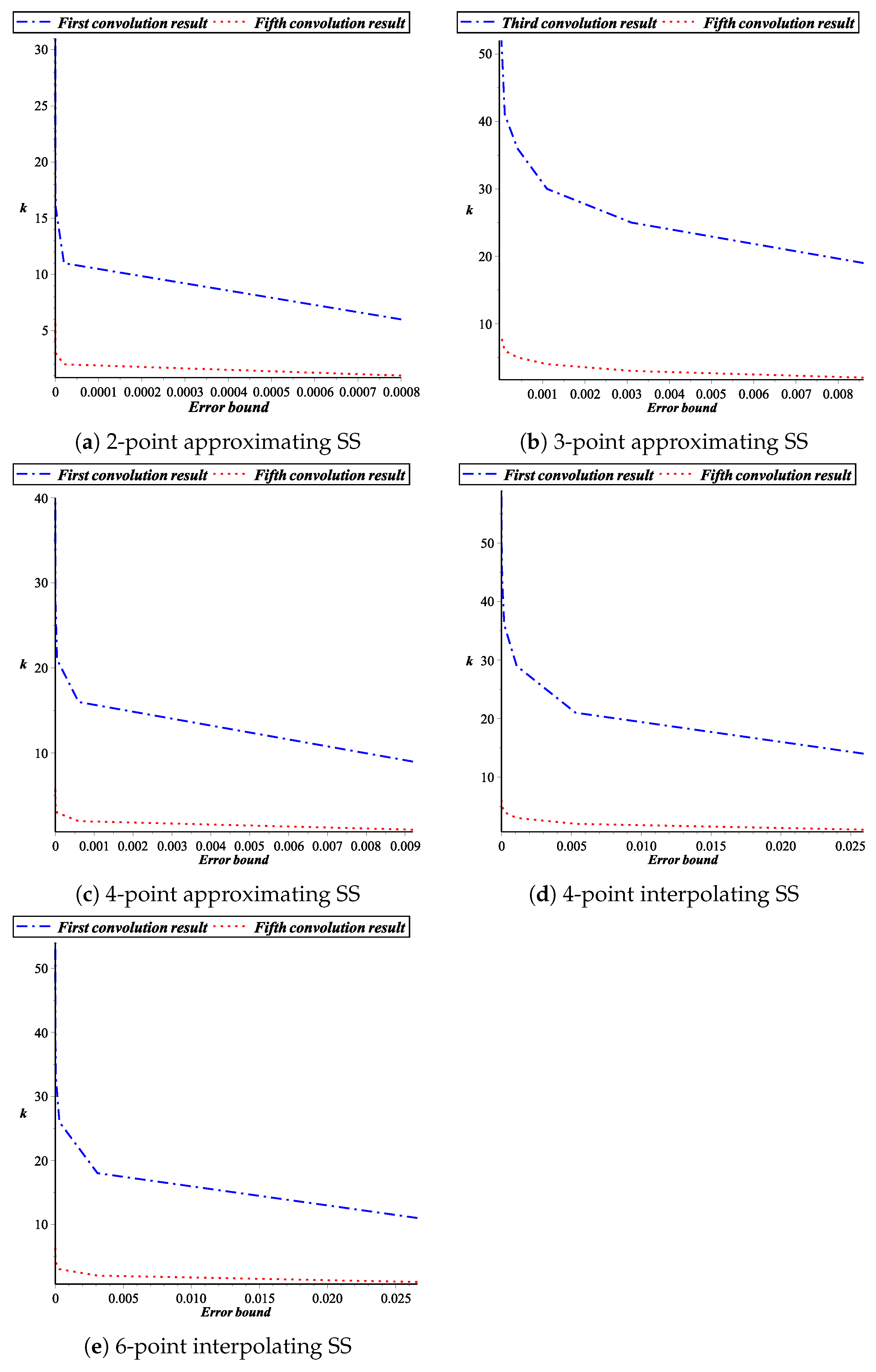
3. Subdivision Depth for Binary Subdivision Curves

Now firstly, the modified technique for finding the error bounds is presented. Secondly, an altered subdivision depth computation technique based on the proposed error bounds is demonstrated with the help of tables.

Theorem 1.

Consider $f_i^0,i\in \mathbb{Z}$ to be the control polygon and $f_i^k$ to be the values for non-negative integers recursively described by $\left(1\right)$ together with mask condition $\left(2\right)$. Suppose $F^k$ denotes the initial at the points $\left\{f_i^k\right\}$. Then after two successive iterations the error bounds between k and $k+1$ stage is

$$\begin{array}{c}\hfill \parallel F^{k+1}-F^k{\parallel }_{\infty }\le \gamma \beta D_{k_0},\end{array}$$

(23)

where $D_{k_0},k_0\ge 1$ defined in (15) and $\beta ={\displaystyle \underset{i}{max}}∥\Delta p_i^0∥,$

$$\begin{array}{c}\hfill \gamma =max\left({\displaystyle \sum _{j=0}^{t-1}}\left|{\tilde{a}}_{0,j}\right|,{\displaystyle \sum _{j=0}^{t-1}}\left|{\tilde{a}}_{1,j}\right|\right),{\tilde{a}}_{0,j}={\displaystyle \sum _{i=j+1}^t}{a}_{0,i},\\ \hfill {\tilde{a}}_{1,0}={\displaystyle \sum _{i=1}^t}{a}_{1,i}-\frac{1}{2},{\tilde{a}}_{1,j}={\displaystyle \sum _{i=j+1}^t}{a}_{1,i},j\ne 0.\end{array}$$

Theorem 2.

Under the same conditions used in Theorem 1, let $F^{\infty }$ be the limit curve associated with the subdivision process, then

$${∥F^{\infty }-F^k∥}_{\infty }\le \gamma \beta \left(\frac{D_{k_0}^k}{1-D_{k_0}}\right),$$

(24)

where $k_0\ge 1$ be a natural number, such that $D_{k_0}<1$.

Remark 1.

In this paper $D_{k_0}$ for $k_0=1$ is equal to δ defined in [4]. Note that in [4], if $\delta >1$ then the error bounds can not be computed. But by [12] and by using our technique, we increase the value of $k_0$ until $D_{k_0}$ becomes less than one.

Theorem 3.

Let k be the subdivision depth and let ${\nabla }^k$ be the error bound between binary subdivision curve $F^{\infty }$ and its k-level control polygon $F^k$. For arbitrary $ϵ>0$, if

$$k\ge {log}_{D_{k_0}^{-1}}\left(\frac{\gamma \chi }{ϵ(1-D_{k_0})}\right),$$

(25)

then ${\nabla }^k\le ϵ$.

Proof. 

Let ${\nabla }^k$ be the distance between limit curve $F^{\infty }$ and control polygon $F^k$ at the k-th subdivision level, then

$${\nabla }^k={∥F^{\infty }-F^k∥}_{\infty }\le \gamma \beta \left(\frac{D_{k_0}^k}{1-D_{k_0}}\right).$$

(26)

To obtain the given error tolerance $ϵ>0$, the subdivision depth k satisfies the following relation, which is in inequality form as

$$k\ge {log}_{D_{k_0}^{-1}}\left(\frac{\gamma \chi }{ϵ(1-D_{k_0})}\right),$$

(27)

then ${\nabla }^k\le ϵ$.

Hence, this completes the proof. □

Application for Univariate Case

Here, we present some numerical examples to compute subdivision depths of binary SSs for curves. The associated constants $D_{k_0},k_0\ge 1$ defined in (15) of some binary subdivision curves are shown in

Table 1. Associated constants of binary subdivision schemes (SSs).

Scheme/${\mathit{D}}_{{\mathit{k}}_0}$	${\mathit{D}}_1=\mathit{\delta }$	${\mathit{D}}_2$	${\mathit{D}}_3$	${\mathit{D}}_4$	${\mathit{D}}_5$
2-point scheme [14]	0.50000	0.25000	0.12500	0.06250	0.03125
3-point scheme [15]	1.50000	1.03125	0.83203	0.52685	0.36584
4-point scheme [16]	0.65625	0.36829	0.21610	0.12153	0.06912
4-point scheme [17]	0.80800	0.55800	0.40343	0.28765	0.20595
6-point scheme [18]	0.74200	0.44218	0.28589	0.18321	0.11768

.

Example 1.

Consider the 2-point Chaikin’s binary SS [14]:

$$\begin{array}{c}\hfill p_{2i}^{k+1}=\frac{3}{4}{p}_i^k+\frac{1}{4}{p}_{i+1}^k,\\ \hfill p_{2i+1}^{k+1}=\frac{1}{4}{p}_i^k+\frac{3}{4}{p}_{i+1}^k.\end{array}$$

(28)

Its subdivision depth by Theorem 3 for $D_{k_0},k_0\ge 1$ (computed in Table 1) are shown in

Table 2. Subdivision depth of 2-point binary subdivision curve.

${\mathit{D}}_{{\mathit{k}}_0}$/$\mathit{ϵ}$	0.0008	0.00002	$7.87\times {10}^{-7}$	$2.46\times {10}^{-8}$	$7.69\times {10}^{-10}$	$2.40\times {10}^{-11}$
$D_1=\delta$	6	11	16	21	26	31
$D_2$	3	5	8	10	13	15
$D_3$	1	3	5	7	8	10
$D_4$	1	3	4	5	6	8
$D_5$	1	2	3	4	5	6

. From this table, we see that as $k_0$ increases the subdivision depth decreases. This shows that the sharp depth can be obtained by using our technique. In other words, we need a smaller number of iterations to get the sharp depth compared to the technique of [11]. For example, by [11], it needs thirty one iterations for $ϵ=2.40\times {10}^{-11}$, but using our technique, it needs only six iterations corresponding to $D_5$, which are shown in Figure 1a.

Example 2.

Consider the 3-point approximating SS [15]:

$$\begin{array}{ccc}\hfill f_{2i}^{k+1}& =& \frac{1}{2}{f}_{i+1}^k+\frac{1}{2}{f}_{i+2}^k,\hfill \\ \hfill f_{2i+1}^{k+1}& =& \frac{1}{8}{f}_i^k+\frac{3}{4}{f}_{i+1}^k+\frac{1}{8}{f}_{i+2}^k.\hfill \end{array}$$

(29)

From

Table 3. Subdivision depth of 3-point binary subdivision curve.

${\mathit{D}}_{{\mathit{k}}_0}$/$\mathit{ϵ}$	0.0086	0.0031	0.0011	0.0004	0.0001	$5.67\times {10}^{-5}$	$2.07\times {10}^{-5}$
$D_3$	19	25	30	36	41	47	52
$D_4$	4	5	7	9	10	12	13
$D_5$	2	3	4	5	6	7	8

, $D_1>1$ and $D_2>1$, so error bounds cannot be computed by [4]. Consequently, it is not possible to compute subdivision depths. In this case, we increase the value of $k_0$ until $D_{k_0}<1$. The subdivision depths of the 3-point scheme are shown in Table 3 at different values of error tolerance. It is also demonstrated with the help of Figure 1b.

Example 3.

The initial polygon have values $f_i^k,k\ge 1$ by following the 4-point approximating binary SS [14] with subdivision mask

$$\begin{array}{c}\hfill (a_{0,0},a_{0,1},a_{0,2},a_{0,3})=\left(-\frac{7}{128},\frac{105}{128},\frac{35}{128},-\frac{5}{128}\right),\\ \hfill (a_{1,0},a_{1,1},a_{1,2},a_{1,3})=\left(-\frac{5}{128},\frac{35}{128},\frac{105}{128},-\frac{7}{128}\right).\end{array}$$

(30)

Its subdivision depths by using Theorem 3 are given in

Table 4. Subdivision depth of 4-point binary subdivision curve.

${\mathit{D}}_{{\mathit{k}}_0}$/$\mathit{ϵ}$	0.0092	0.0006	$4.43\times {10}^{-5}$	$3.06\times {10}^{-6}$	$2.11\times {10}^{-7}$	$1.46\times {10}^{-8}$
$D_1$	9	16	21	28	34	40
$D_2$	3	6	8	11	14	16
$D_3$	2	4	5	7	9	11
$D_4$	1	3	4	5	6	8
$D_5$	1	2	3	4	5	6

. The comparison of the first and fifth convolution results is shown in Figure 1c.

Example 4.

Consider $f_i^0=f_i,i\in \mathbb{Z}$ denotes the initial polygon with values $f_i^k,k\ge 1$, which can be expressed recursively by the 4-point interpolating binary SS [17] with weights

$$\begin{array}{ccc}\hfill (a_{0,0},a_{0,1},a_{0,2},a_{0,3})& =& \left(0,1,0,0\right),\hfill \\ \hfill (a_{1,0},a_{1,1},a_{1,2},a_{1,3})& =& \left(-w,\frac{1}{2}+w,\frac{1}{2}+w,-w\right).\hfill \end{array}$$

(31)

Its subdivision depths are given in

Table 5. Subdivision depth of 4-point binary subdivision curve.

${\mathit{D}}_{{\mathit{k}}_0}$/$\mathit{ϵ}$	0.0259	0.0053	0.00109	0.0002	$4.66\times {10}^{-5}$	$9.59\times {10}^{-6}$	$1.97\times {10}^{-6}$
$D_1$	14	21	29	36	44	51	59
$D_2$	4	6	9	12	15	17	20
$D_3$	2	4	6	7	9	11	12
$D_4$	1	3	4	5	6	8	9
$D_5$	1	2	3	4	5	6	7

. It is also illustrated with the help of the graph given in Figure 1d.

Example 5.

Given the initial polygon $f_i^0=f_i,i\in \mathbb{Z}$ with values $f_i^k,k\ge 1$ can be expressed recursively by the 6-point interpolating binary SS [18] as

$$\begin{array}{ccc}\hfill (a_{0,0},a_{0,1},a_{0,2},a_{0,3},a_{0,4},a_{0,5})& =& \left(0,0,1,0,0,0\right),\hfill \\ \hfill (a_{1,0},a_{1,1},a_{1,2},a_{1,3},a_{1,4},a_{1,5})& =& \left(w,-\frac{1}{16}-3w,\frac{9}{16}+2w,\frac{9}{16}+2w,-\frac{1}{16}-3w,w\right).\hfill \end{array}$$

(32)

In

Table 6. Subdivision depth of 6-point binary subdivision curve.

${\mathit{D}}_{{\mathit{k}}_0}$/$\mathit{ϵ}$	0.0266	0.0031	0.0003	$4.35\times {10}^{-5}$	$5.12\times {10}^{-6}$	$6.02\times {10}^{-7}$	$7.09\times {10}^{-8}$
$D_1$	11	18	26	33	40	47	54
$D_2$	3	6	8	11	14	16	19
$D_3$	2	4	5	7	9	10	12
$D_4$	1	3	4	5	6	8	9
$D_5$	1	2	3	4	5	6	7

, subdivision depths are presented and its performance is shown in Figure 1e.

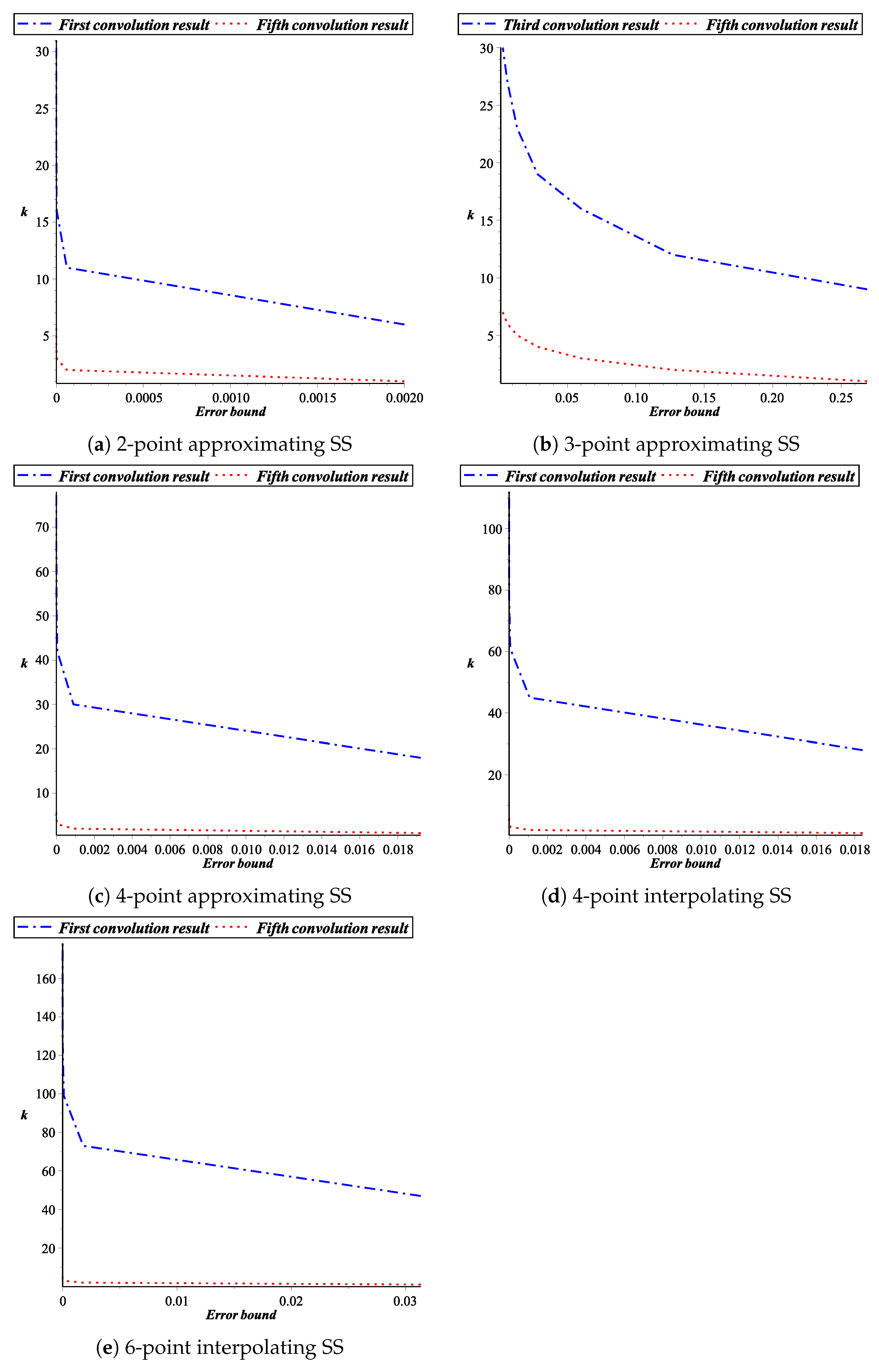
4. Subdivision Depth for Binary Subdivision Surfaces

In the following section, firstly we calculate error bounds for subdivision surfaces. Secondly, we use these error bounds to compute subdivision depths.

Theorem 4.

Consider $f_{i,j}^0,i,j\in \mathbb{Z}$ to be the initial polygon and $f_{i,j}^k$ to be the values for all non-negative integers recursively given in $\left(5\right)$ along with the condition $\left(6\right)$. Also let $F^k$ be the representation of the polygon at the points $f_{i,j}^k$. Then the error bounds of two successive refinements between the level k and $k+1$ by using the same technique given in [4] is

$$\begin{array}{c}\hfill \parallel F^{k+1}-F^k{\parallel }_{\infty }\le \left(\eta {\beta }_1+\tau {\beta }_2+\xi {\beta }_3\right)F_{k_0}{G}_{k_0},\end{array}$$

(33)

where $F_{k_0},G_{k_0},k_0\ge 1$ defined in (21) and (22), ${\beta }_t={max}_{i,j}\parallel {\Delta }_{i,j}^{0,t}\parallel$, t = 1,2,3,

$${\Delta }_{i,j}^{k,1}=p_{i+1,j}^k-p_{i,j}^k,{\Delta }_{i,j}^{k,2}=p_{i,j+1}^k-p_{i,j}^k,{\Delta }_{i,j}^{k,3}=p_{i+1,j+1}^k-p_{i,j+1}^k,$$

and η, τ and ξ are defined by

$$\begin{array}{c}\hfill {\eta }_1=\left|a_{0,0}\right|\left({\displaystyle \sum _{r=1}^t}\left|a_{0,r}\right|+{\displaystyle \sum _{q=1}^{t-1}}\left|{\tilde{a}}_{0,q}\right|\right),{\eta }_2=\left|a_{0,0}\right|\left({\displaystyle \sum _{r=1}^t}\left|a_{1,r}\right|+{\displaystyle \sum _{q=1}^{t-1}}\left|{\tilde{a}}_{1,q}\right|\right)+\frac{1}{2},\\ \hfill {\eta }_3=\left|a_{1,0}\right|\left({\displaystyle \sum _{r=1}^t}\left|a_{0,r}\right|+{\displaystyle \sum _{q=1}^{t-1}}\left|{\tilde{a}}_{0,q}\right|\right),{\eta }_4=\left|a_{1,0}\right|\left({\displaystyle \sum _{r=1}^t}\left|a_{1,r}\right|+{\displaystyle \sum _{q=1}^{t-1}}\left|{\tilde{a}}_{1,q}\right|\right)+\frac{1}{4},\end{array}$$

$$\begin{array}{c}\hfill {\tau }_1={\displaystyle \sum _{r=1}^t}\left|a_{0,r}\right|+{\displaystyle \sum _{m=0}^t}\left|a_{0,m}\right|{\displaystyle \sum _{q=1}^{t-1}}\left|{\tilde{a}}_{0,q}\right|,{\tau }_2={\displaystyle \sum _{r=1}^t}\left|a_{0,r}\right|+{\displaystyle \sum _{m=0}^t}\left|a_{1,m}\right|{\displaystyle \sum _{q=1}^{t-1}}\left|{\tilde{a}}_{0,q}\right|,\\ \hfill {\tau }_3={\displaystyle \sum _{r=1}^t}\left|a_{1,r}\right|+{\displaystyle \sum _{m=0}^t}\left|a_{0,m}\right|{\displaystyle \sum _{q=1}^{t-1}}\left|{\tilde{a}}_{1,q}\right|+\frac{1}{2},{\tau }_4={\displaystyle \sum _{r=1}^t}\left|a_{1,r}\right|+{\displaystyle \sum _{m=0}^t}\left|a_{1,m}\right|{\displaystyle \sum _{q=1}^{t-1}}\left|{\tilde{a}}_{1,q}\right|+\frac{1}{2},\end{array}$$

$$\begin{array}{c}\hfill {\xi }_1={\displaystyle \sum _{r=1}^t}\left|a_{0,r}\right|\left({\displaystyle \sum _{r=1}^t}\left|a_{0,r}\right|+{\displaystyle \sum _{q=1}^{t-1}}\left|{\tilde{a}}_{0,q}\right|\right),{\xi }_2={\displaystyle \sum _{r=1}^t}\left|a_{0,r}\right|\left({\displaystyle \sum _{r=1}^t}\left|a_{1,r}\right|+{\displaystyle \sum _{q=1}^{t-1}}\left|{\tilde{a}}_{1,q}\right|\right),\\ \hfill {\xi }_3={\displaystyle \sum _{r=1}^t}\left|a_{1,r}\right|\left({\displaystyle \sum _{r=1}^t}\left|a_{0,r}\right|+{\displaystyle \sum _{q=1}^{t-1}}\left|{\tilde{a}}_{0,q}\right|\right),{\xi }_4={\displaystyle \sum _{r=1}^t}\left|a_{1,r}\right|\left({\displaystyle \sum _{r=1}^t}\left|a_{1,r}\right|+{\displaystyle \sum _{q=1}^{t-1}}\left|{\tilde{a}}_{1,q}\right|\right)+\frac{1}{4}.\end{array}$$

Finally,

$$\begin{array}{c}\hfill \eta =max\{{\eta }_t;t=1,2,3,4\},\tau =max\{{\tau }_t;t=1,2,3,4\},\xi =max\{{\xi }_t;t=1,2,3,4\}.\end{array}$$

Theorem 5.

Under the same circumstances used in Theorem 4. Let $F^{\infty }$ be the limit surface associated with the subdivision process. Then

$$\parallel F^{\infty }-F^k{\parallel }_{\infty }\le (\eta {\beta }_1+\tau {\beta }_2+\xi {\beta }_3)\left(\frac{{\left(F_{k_0}{G}_{k_0}\right)}^k}{1-F_{k_0}{G}_{k_0}}\right),$$

(34)

where $k_0\ge 1$ is a natural number, such that $F_{k_0}{G}_{k_0}<1$.

Remark 2.

Again $F_1{G}_1$ is also equal to δ which is defined in [4].

Theorem 6.

Let k be the subdivision depth and let ${\nabla }^k$ be the error bound between binary subdivision surface $F^{\infty }$ and its k-level control polygon $F^k$. For arbitrary $ϵ>0$, if

$$k\ge {log}_{{\left(F_{k_0}{G}_{k_0}\right)}^{-1}}\left(\frac{\psi }{ϵ(1-F_{k_0}{G}_{k_0})}\right),$$

(35)

then ${\nabla }^k\le ϵ$.

Proof. 

Let ${\nabla }^k$ denote the distance between limit curve $F^{\infty }$ and initial curve (polygon) $F^k$ at the k-th level. Then

$${\nabla }^k={\parallel F^{\infty }-F^k\parallel }_{\infty }\le (\eta {\beta }_1+\tau {\beta }_2+\xi {\beta }_3)\left(\frac{{\left(F_{k_0}{G}_{k_0}\right)}^k}{1-F_{k_0}{G}_{k_0}}\right).$$

(36)

To obtain given error tolerance $ϵ>0$ the subdivision depth k satisfies the following inequality:

$$k\ge {log}_{{\left(F_{k_0}{G}_{k_0}\right)}^{-1}}\left(\frac{\psi }{ϵ(1-F_{k_0}{G}_{k_0})}\right),$$

(37)

then ${\nabla }^k\le ϵ$.

This completes the proof. □

Application for Bivariate Case

Here, we present some numerical examples to compute subdivision depths for subdivision surfaces. The associated constants $F_{k_0}{G}_{k_0},k_0\ge 1$ for some binary subdivision surfaces by using (21) and (22) are shown in

Table 7. Associated constants of binary SSs.

Scheme/ ${\mathit{F}}_{{\mathit{k}}_0}{\mathit{D}}_{{\mathit{k}}_0}$	${\mathit{F}}_1{\mathit{G}}_1=\mathit{\delta }$	${\mathit{F}}_2{\mathit{G}}_2$	${\mathit{F}}_3{\mathit{G}}_3$	${\mathit{F}}_4{\mathit{G}}_4$	${\mathit{F}}_5{\mathit{G}}_5$
2-point scheme [14]	0.50000	0.25000	0.12500	0.06250	0.03125
3-point scheme [15]	1.50000	1.00000	0.81250	0.60937	0.47265
4-point scheme [16]	0.77930	0.40902	0.20020	0.09959	0.04953
4-point scheme [17]	0.84500	0.43741	0.22635	0.11557	0.05801
6-point scheme [18]	0.89780	0.45218	0.23205	0.11764	0.05902

. We see that the values of $F_{k_0}{G}_{k_0}$ decrease with the increase of $k_0$. This is the advantage of our approach.

Example 6.

Given the initial polygon $F_{i,j}^0=F_{i,j},i,j\in \mathbb{Z}$ and the values $F_{i,j}^k,k\ge 1$ be described recursively by the tensor product of (28), then the subdivision depths for $F_{k_0}{G}_{k_0},k_0\ge 1$ by using Theorem 35 are shown in

Table 8. Subdivision depth of 2-point binary subdivision surface.

${\mathit{F}}_{{\mathit{k}}_0}{\mathit{G}}_{{\mathit{k}}_0}$/$\mathit{ϵ}$	0.0020	0.00006	$1.96\times {10}^{-6}$	$6.15\times {10}^{-8}$	$1.92\times {10}^{-9}$	$6.008\times {10}^{-11}$
$F_1{G}_1$	6	11	16	21	26	31
$F_2{G}_2$	3	5	8	10	13	15
$F_3{G}_3$	2	3	5	7	8	10
$F_4{G}_4$	1	3	4	5	6	8
$F_5{G}_5$	1	2	3	4	5	6

and the comparison of the first and fifth convolution result is shown in Figure 2a.

Example 7.

Consider the tensor product of the 3-point approximating SS defined in (29). The mask of SS satisfies $F_{k_0}{G}_{k_0}<1$, for $k_0\ge 3$. Therefore its subdivision depths can be computed at different values of error tolerance which are shown in

Table 9. Subdivision depth of the 3-point binary subdivision surface.

${\mathit{F}}_{{\mathit{k}}_0}{\mathit{G}}_{{\mathit{k}}_0}$/$\mathit{ϵ}$	0.2688	0.1270	0.06007	0.0283	0.0134	0.0063	0.0029
$F_3{G}_3$	9	12	16	19	23	27	30
$F_4{G}_4$	2	4	5	7	8	10	11
$F_5{G}_5$	1	2	3	4	5	6	7

. Here, the comparison of the third and fifth convolutions is demonstrated in Figure 2b.

Example 8.

Given that $f_{i,j}^0=f_{i,j},i,j\in \mathbb{Z}$, let the values $f_{i,j}^k,k\ge 1$ be described recursively by the tensor product of (30). Then the subdivision depths for $F_{k_0}{G}_{k_0},k_0\ge 1$ by using Theorem 35 are shown in

Table 10. Subdivision depth of 4-point binary subdivision surface.

${\mathit{F}}_{{\mathit{k}}_0}{\mathit{G}}_{{\mathit{k}}_0}$/$\mathit{ϵ}$	0.0192	0.0009	$4.72\times {10}^{-5}$	$2.33\times {10}^{-6}$	$1.15\times {10}^{-7}$	$5.73\times {10}^{-9}$
$F_1{G}_1$	18	30	42	54	66	78
$F_2{G}_2$	4	7	10	14	17	21
$F_3{G}_3$	2	4	6	8	9	11
$F_4{G}_4$	1	3	4	5	7	8
$F_5{G}_5$	1	2	3	4	5	6

which is illustrated in Figure 2c.

Example 9.

Consider the initial control polygon $f_{i,j}^0=f_{i,j},i,j\in \mathbb{Z}$ and let the values $f_{i,j}^k$ for all positive integers be defined recursively by the tensor product of (31). Then the subdivision depths for $F_{k_0}{G}_{k_0},k_0\ge 1$ are shown in

Table 11. Subdivision depth of 4-point binary subdivision surface.

${\mathit{F}}_{{\mathit{k}}_0}{\mathit{G}}_{{\mathit{k}}_0}$/$\mathit{ϵ}$	0.0184	0.00107	$6.21\times {10}^{-5}$	$3.6\times {10}^{-6}$	$2.09\times {10}^{-7}$	$1.21\times {10}^{-8}$
$F_1{G}_1$	28	45	61	78	95	112
$F_2{G}_2$	4	7	11	14	18	21
$F_3{G}_3$	2	4	6	8	10	12
$F_4{G}_4$	1	3	4	5	7	8
$F_5{G}_5$	1	2	3	4	5	6

. It is also presented with the help of the graph in Figure 2d.

Example 10.

Given the initial control polygon $f_{i,j}^0=f_{i,j},i,j\in \mathbb{Z}$ and that the values $f_{i,j}^k,k\ge 1$ can be described recursively by the tensor product of (32), then in

Table 12. Subdivision depth of 6-point binary subdivision surface.

${\mathit{F}}_{{\mathit{k}}_0}{\mathit{G}}_{{\mathit{k}}_0}$/$\mathit{ϵ}$	0.0313	0.0018	0.0001	$6.44\times {10}^{-6}$	$3.80\times {10}^{-7}$	$2.24\times {10}^{-8}$
$F_1{G}_1$	47	73	99	126	152	178
$F_2{G}_2$	4	8	11	15	18	22
$F_3{G}_3$	2	4	6	8	10	12
$F_4{G}_4$	1	3	4	5	7	8
$F_5{G}_5$	1	2	3	4	5	6

, subdivision depths for $F_{k_0}{G}_{k_0},k_0\ge 1$ are presented and a graphical representation is shown in Figure 2e.

5. Conclusions

In this paper, the modified version of the numerical algorithm of [4,11,12] have been presented to compute the subdivision depths of the SSs for curves and surfaces design. Our algorithm can be used when the computation techniques of [4,11] fail. Moreover, we a smaller number of iterations to get the sharp subdivision depth compared to the existing algorithm. The proposed method is an efficient way of estimating subdivision depths for binary subdivision curves and surfaces.

References

1. Barnhill, R.E.; Riesenfeld, R.F. Computer Aided Geometric Design; Academic Press: New York, NY, USA, 1974. [Google Scholar]
2. Faux, I.; Pratt, M. Computational Geometry for Design and Manufacture; Ellis Horwood: New York, NY, USA, 1979. [Google Scholar]
3. Huawei, W.; Youjiang, G.; Kaihuai, Q. Error estimation for Doo-Sabin surfaces. Prog. Nat. Sci. 2002, 12, 697–700. [Google Scholar]
4. Mustafa, G.; Chen, F.; Deng, J. Estimating error bounds for binary subdivision curves/surfaces. J. Comput. Appl. Math. 2006, 193, 596–613. [Google Scholar] [CrossRef] [Green Version]
5. Mustafa, G.; Hashmi, S.; Faheem, K. Estimating error bounds for non-stationary binary subdivision curves/surfaces. J. Inf. Comput. Sci. 2007, 2, 179–190. [Google Scholar]
6. Mustafa, G.; Deng, J. Estimating error bounds for ternary subdivision curve/surfaces. J. Comput. Math. 2007, 25, 473–484. [Google Scholar]
7. Mustafa, G.; Hashmi, S. Estimating error bounds for quaternary subdivision schemes. J. Math. Anal. Appl. 2009, 358, 159–167. [Google Scholar]
8. Mustafa, G.; Hashmi, S.; Noshi, N.A. Estimating error bounds for tensor product binary subdivision volumetric model. Int. J. Comput. Math. 2006, 83, 879–903. [Google Scholar] [CrossRef]
9. Mustafa, G.; Hashmi, S.; Faheem, K. Error bounds for 3 subdivision surfaces. J. Univ. Sci. Technol. China 2009, 39, 1–9. [Google Scholar]
10. Mustafa, G.; Hashmi, S.; Faheem, K. Subdivision depth for triangular surfaces. Alex. Eng. J. 2016, 55, 1647–1653. [Google Scholar] [CrossRef] [Green Version]
11. Mustafa, G.; Hashmi, S. Subdivision depth computation for n-ary subdivision curves/surfaces. J. Vis. Comput. 2010, 26, 841–851. [Google Scholar] [CrossRef] [Green Version]
12. Moncayo, M.; Amat, S. Error bounds for a class of subdivision schemes based on the two-scale refinement equation. J. Comput. Appl. Math. 2011, 236, 265–278. [Google Scholar] [CrossRef] [Green Version]
13. Dyn, N.; Gregory, A.; Levin, D. Analysis of uniform binary subdivision scheme for curve design. Constr. Approx. 1991, 7, 127–147. [Google Scholar] [CrossRef] [Green Version]
14. Chaikin, G.M. An algorithm for high speed curve generation. Comput. Graph. Image Process. 1974, 3, 346–349. [Google Scholar] [CrossRef]
15. Dyn, N.; Levin, D.; Micchelli, C.A. Using parameters to increase smoothness of curves and surfaces generated by subdivision. Comput. Aided Geom. Des. 1990, 7, 129–140. [Google Scholar] [CrossRef]
16. Dyn, N.; Floater, M.S.; Hormann, K. A four-point subdivision scheme with fourth order accuracy and its extensions. In Mathematical Methods for Curves and Surfaces: Modern Methods in Mathematics; Springer: Troms, Norway, 2004; pp. 145–156. [Google Scholar]
17. Dyn, N.; Levin, D.; Gregory, J.A. A 4-Point Interpolatory SS for Curve Design. Comput. Aided Geom. Des. Acad. Press. 1987, 4, 257–268. [Google Scholar] [CrossRef]
18. Weissman, A. A 6-Point Interpolatory Subdivision Scheme for Curve Design. Master’s Thesis, Tel Aviv University, Tel Aviv-Yafo, Israel, 1990. [Google Scholar]
Figure 1. The performance of different subdivision schemes for univariate case. Here k presents the subdivision depth (level of subdivision process) obtained after user-specified error tolerance.
Symmetry 12 00066 g001
Figure 2. Presents the performance of different subdivision schemes for bivariate case. Here k presents the subdivision depth (level of subdivision process) obtained after user-specified error tolerance.
Symmetry 12 00066 g002