Abstract
Small-angle scattering (SAS; X-rays, neutrons, light) is being increasingly used to better understand the structure of fractal-based materials and to describe their interaction at nano- and micro-scales. To this aim, several minimalist yet specific theoretical models which exploit the fractal symmetry have been developed to extract additional information from SAS data. Although this problem can be solved exactly for many particular fractal structures, due to the intrinsic limitations of the SAS method, the inverse scattering problem, i.e., determination of the fractal structure from the intensity curve, is ill-posed. However, fractals can be divided into various classes, not necessarily disjointed, with the most common being random, deterministic, mass, surface, pore, fat and multifractals. Each class has its own imprint on the scattering intensity, and although one cannot uniquely identify the structure of a fractal based solely on SAS data, one can differentiate between various classes to which they belong. This has important practical applications in correlating their structural properties with physical ones. The article reviews SAS from several fractal models with an emphasis on describing which information can be extracted from each class, and how this can be performed experimentally. To illustrate this procedure and to validate the theoretical models, numerical simulations based on Monte Carlo methods are performed.
1. Introduction
Small-angle scattering (SAS; X-rays, neutrons, light) is a widely used innovative technique for an efficient characterization of the structure of disordered materials at nano- and micro-scales [1,2]. With the recent advances of its derivative techniques, i.e., grazing-incidence [3], anomalous [4], scanning [5] or magnetic [6] SAS, the range of applications has been greatly extended. This includes now a much larger class of hierarchical materials, i.e., materials in which the structural elements themselves have a structure, such as biological macromolecules [1,7,8,9], polymers [10,11,12,13], composites [14,15,16,17] or cellular solids [18,19,20].
It is well-known that in fractal-based materials, the structural hierarchy and the geometric symmetry within a single structure play an important role in determining their bulk and surface properties. Common applications of such materials include enhancing: the lithium storage performance of CuO nanomaterials with surface fractal characteristics [21], the rheological behavior of fractal-like aggregates in polymer nanocomposites [22], the compatibility and interfacial reactivity of high-performance layered silicate/epoxy nanocomposites [23], the tensile modulus and strength in carbon nanotube fibers with mesoporous crystalline structure [24] or the electrocatalytic activity, durability and stability in Sierpinski gasket-like Pt–Ag octahedral alloy nanocrystals [25]. In addition, the fractal structure [26], also gives rise to quantum effects in various materials such as in plasmonic structures with sub-nanometer gaps [27] or in organometal halide perovskite nanoplatelets [28]. This dependence of the quantum effects and bulk properties on the fractal structure, can be attributed to the interplay between regular and chaotic dynamics of particles, confined in fractal-like regions. This interplay in classical and quantum systems leads to the emergence of dynamical symmetries, and are related to the existence of conserved quantities of the dynamics and integrability under certain conditions [29].
Therefore, understanding the influence of the fractal structure on physical properties and their evolution, can guide the preparation of advanced materials tailored for specific applications. Within this context, development of theoretical models for SAS data analysis and interpretation form the first steps in elucidating the structure-bulk properties relationship. However, the evolution of their properties, is usually determined by complex quantum mechanical models.
In SAS analysis, one of the key issues is the development of models that allow extracting the most important structural parameters from a given set of SAS measurements. Due to technological limitations, until several years ago almost all measurements were performed on random fractals, i.e., on structures where only statistical properties remain invariant at various magnifications, such as clusters generated by diffusion-limited aggregation (DLA). Thus, parameter-extraction procedures concerned obtaining only the fractal dimensions or (see below), and the inner and outer fractal cutoffs l, and respectively [30,31,32,33,34,35,36]. While the fractal dimension is related to the self-similarity property under scale transformations [26], the two cutoffs set the range in which this self-similarity can be observed. For physical samples, the inner cutoff is defined by the size of the building blocks that make up the fractal (typically atoms or molecules). The outer cutoff is defined by the largest distance separating two points inside the fractal.
The fractal dimension is captured in the modeling process by writing the scattering intensity, such as [37]:
This is a simple power-law decay on a double logarithmic scale within a given q-range limited by reciprocal fractal outer and inner cutoffs , and respectively , i.e., when . It is also known in the literature as the fractal region. Here, q is the module of the scattering vector, , and are the surface, mass and respectively the pore fractal dimensions, and d is the Euclidean dimension of the space in which the fractal is embedded. In the case of surface fractals , and the scattering intensity reduces to [38]. For mass fractals , and , and [39], while for pore fractals and , and thus [40]. Therefore, by using Equation (1) one can obtain the fractal dimension from the slope () of the experimental scattering curve. Moreover, one can differentiate between mass and surface fractals, i.e., if the measured slope is then the sample is a mass fractal, while if , the sample is a surface fractal.
To obtain the outer fractal cutoff , Equation (1) is extended by adding a properly weighted exponential term which gives rise to a region (also known as Guinier region) where at . Then, the position of the transition point gives an estimation of fractal radius of gyration, which in turn is a measure of its outer cutoff [41,42]. The inner fractal cutoff l is obtained by addition of a second exponential term and of a power-law decay at . Then, the position of is related to the radius of gyration of the smallest building block composing the fractal [41,42]. Moreover, by considering a succession of power-law decays interleaved with Guinier regions, one can describe hierarchically structured systems. This succession forms the basis of Beaucage [43,44] and Guinier–Porod [45] models, which are widely used as empirical models to analyze SAS data from random fractal and particulate systems, such as those occurring in some amphiphilic triblock polyelectrolytes [46], rocks [47], fertilizers encapsulated by starch-based superabsorbent polymers [48], silica-filled silicone rubber [49], aerosol nanoparticles [50] or micro/nano-sized TATB crystallites [51].
However, recent advances in materials science and nanotechnology allows fabrication of deterministic fractal materials with predefined structures, i.e., structures where an intrinsic pattern repeats itself exactly under scaling, such as: Sierpinski triangular [52,53,54], supramolecular [25,55], octahedral [56] or Cantor fractals [57]. In addition, theoretical developments in SAS from deterministic fractals have shown that the corresponding intensity curves are characterized by a much more complex behavior, as compared to scattering from random fractals. The main difference is that in the former case, the simple power-law decay is replaced by a generalized power-law decay, where maxima and minima superimposed on a monotonically decreasing curve [58,59,60]. Also, the complexity of the patterns formed by these maxima and minima increases with the magnitude of the scattering vector q. Generally, both features arise as an effect of two competing symmetries present in a deterministic fractal. First, there is dilation invariance symmetry, which is responsible for the power-law decay. Second, there is geometric symmetry, which is the source of maxima splitting as q increases. These two symmetry-effects are the defining characteristics of SAS from deterministic fractals, and are generally used to differentiate them from random fractals [58].
Although separating these effects from SAS intensity is not an easy task, some general guidelines for extracting additional structural parameters have been provided for various types of deterministic fractals. In the case of SAS from deterministic mass fractals one can extract [58]:
- The fractal dimension , from the generalized power-law decay:
- The fractal scaling factor , from the period of the scattering curve on a double logarithmic scale,
- The number of fractal iterations m, equal to the number of the main minima,
- The inner and outer fractal cutoffs from the beginning and the end of periodicity region, i.e., from fractal regime,
- The total number of basic objects composing the fractal, from the relation .
For mass fractals, the log-periodicity of the scattering curve arises from the self-similarity of distances between the basic objects composing the fractal. In the case of deterministic surface fractals one can extract basically the same information [60]. However, the nature of log-periodicity in the fractal region is different, and arises from the self-similarity of sizes of the basic objects. In the case of deterministic fat fractals, i.e., fractals in which the scaling factor is not constant, but it increases after a given number of iterations, it was shown that one can obtain the fractal dimensions and scaling factors at each scale [59,61]. In the case of deterministic multifractals with two scaling factors, i.e., fractals with various scaling factors at the same scale, it was shown that under certain conditions, one can also obtain both scaling factors from SAS curves [62].
In this survey are presented and discussed the latest theoretical advances useful for differentiating between random, deterministic mass, surface, fat and multifractals, from SAS data. Detailed “receipts” are provided that show how to extract the structural parameters about each fractal type. They are subsequently applied to numerical data generated from Monte Carlo methods. To this aim, the pair- distance distribution function (pddf), the form and structure factors are calculated. The importance of preparing samples with a high degree of monodispersity for a clear and unambiguous description of experimental SAS data, is highlighted by studying the influence on the scattering curve of a log-normal distribution of the fractal size.
The paper is structured as follows. Section 2 presents the theoretical background required for a proper understanding of the results discussed thereafter. Here, the main properties of fractals, of SAS technique and Monte Carlo simulations relevant to SAS from fractals are described. In Section 3 are introduced the main types of fractals together with representative models. Analytic expressions of the form and structure factors are derived and compared with results from Monte Carlo simulations. The main conclusions and prospects for future theoretical developments are summarized in Section 4.
2. Theoretical Background
2.1. Fractals
Mathematically, characterization of fractals requires a rigorous definition of the fractal (Hausdorff) dimension [63]. This which involves abstract concepts from measures theory [64]. For this purpose, let us consider S a subset of the n-dimensional Euclidean space, and that the set is a cover of S with , with S. The Hausdorff measure of the set S is defined by taking the infimum over all possible coverings, i.e.,:
Then, the fractal dimension D of the set S is defined by:
This corresponds to the value of for which the Hausdorff measure changes from zero to infinity. When , can take arbitrarily values within this range.
However, in practice is very difficult to apply Equation (3) for determination of the fractal dimension, and therefore one must resort to other methods. A common approach is to determine the variation of the fractal measure M, such as mass, area, volume, or any scalar quantity attached to the fractal support, within a sphere of dimension n and radius r centered on the fractal. For this purpose, we can write [65]:
where . This is known in the literature as the mass-radius relation [65].
Let us consider a fractal of size L composed of balls of size a. Then, the number of balls enclosed by the imaginary sphere of radius r with a ball in the center, is given by [65]:
with . If the fractal is a line then , if it is a smooth surface, , while if the fractal is a regular Euclidean three-dimensional object, then . For , the structure reduces to a set of disconnected points.
In the case of fractals with a scaling factor , one can use the property that at first iteration the fractal consists of k copies of itself, each of size , and write that [65]:
Then, by using Equation (4), one obtains:
which can be used to obtain the fractal dimension D. In the case of fractals with multiple scaling factors and copies with , the above equation can be extended to [65]:
For surface fractals one can write a similar relationship as in Equation (5), and write as [66]:
where represents the area between the boundary of the (rough) surface and the envelope of all spheres of radius r centered on the boundary. Here, is a constant, which is the surface area itself for a smooth surface, i.e., when . Analogous relations as those given by Equation (7) can be written for surface fractals also. For three-dimensional fractals, when the surface is so folded that it almost fulfills all the available space, while when , the surface is almost completely smooth.
The fractal dimensions obtained above are equivalent with the box-counting dimension described in Ref. [26]. This is the single dimension which characterize fractals with a single scaling factor. However, for fractals with multiple scaling factors, a more detailed description of their structure requires determination of additional fractal dimensions. This is achieved by making use of the multifractal formalism [67,68], and in particular of the moment method [69]. Although other methods have been developed for determination of the dimension spectra, the moment method is widely used for its general applicability, including image analysis.
Within this method, one considers an object S covered by a grid of boxes of size l. Let us suppose that the measure determined by the probability of hitting the object in the box is . Therefore, the number of covered boxes N at resolution l is , and the corresponding “partition function” can be written as [70]:
Here, i denotes each individual box, and with , are the hitting probabilities. Then, the generalized dimension spectrum is given by [70]:
The function has a power-law behavior when and , so that . Thus:
where the ratio gives the relative weight of the i-th box.
One of the main property of is that is a monotonically decreasing function, with horizontal asymptotes at and . Therefore, one can describe the scaling properties of the most rarefied, and respectively of the most dense regions in the fractal in terms of and , i.e., the object is heterogeneous (multifractal) if , and homogeneous (simple fractal) otherwise. Also, the box-counting dimension is recovered, at , and is given by [65]:
where is the number of boxes in the minimal cover. At , one obtains which is called the information, i.e.:
and describes how the morphology increases as , i.e., the lower the values of , the less uniform the density. For , Equation (12) gives the two-point correlation dimension , and measures the correlation between pairs of points in each box. The higher the values of the more compact the fractal. As we shall see later, we can extract only the dimension from SAS data.
2.2. Small-Angle Scattering
In SAS, a beam of particles (usually X-ray or neutrons) hit a sample, after which they are scattered elastically at various angles , as shown in Figure 1 [71]. While X-rays are scattered by the electron cloud, neutrons are scattered by nuclei or by the magnetic moments associated with unpaired electron spins in magnetic materials. The structure of the sample is to be determined from the distribution of scattered beam around the beam-stop.
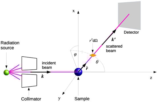
Figure 1.
Overall configuration of a SAS experiment. First, a beam of particles is emitted from a radiation source, and a small fraction pass through the collimator. Then, they hit the sample, and the scattered particles around the beam-stop are recorded. The quantities and denote the incident and, respectively the scattered wave vectors, is the solid angle, and is the unit vector along the beam scattered at angles and [72].
2.2.1. General Background
Basically, one can describe a SAS process by considering that the beam propagates with the wave vector along an axis which coincides with the axis of the collimator with beam opening . Here, is the wavelength. The role of the collimator is to select a monochromatic and well collimated beam, such that it provides a sharp energy spectrum, concentrated at a unique eigenvalue. A detector, placed at a large distance from the sample, records the number of particles passing through a small opening (Figure 1). Let us consider that its position is given by the vector , which is oriented along the direction , and at an angle with respect to the direction of the incident beam. As such, the structure of the scattering particles can be described in terms of the wave vector . To this aim, one introduces the scattering vector defined by [71]:
where = k. Thus, the magnitude of the scattering vector is given by:
Since , and , the previous equation becomes:
Let us consider that an incident beam of neutrons or X-rays is scattered by a sample of volume containing a macroscopic number of objects with scattering lengths . After such an event, the scattering amplitude can be written as [71]:
where is the scattering length density (SLD), are the microscopic objects positions and is the Dirac’s function. In SAS, multiple scattering is neglected, and the scattering intensity , i.e., the differential scattering cross section per unit volume, is expressed as the product between the scattering amplitude and its complex conjugate, i.e., [71]:
Since the positions , and thus SLD, are fixed in time, Equation (19) can be written as [73]:
where is given by:
and represents the autocorrelation function of the deviations of SLD from its mean value , i.e., . Then, the normalized correlation function is defined as [74]:
and where the normalization constant is given by:
Here, is the mean square fluctuation of the density fluctuations about its mean value throughout the sample. Therefore, Equation (20) takes the form:
The function as increases, there are no correlations between fluctuations of and at large , and the integration over the volume can be replaced by an integration over an infinite region. Also, only for small values of , and the properties of depend only on the magnitude of . Therefore, the intensity in Equation (24) becomes:
where the property has been used (see also Equation (29) below). The function depends also on the system’s geometry and gives the probability to find a volume element within the system, at a distance r from another volume element .
2.2.2. Two-Phase Fractal Systems
We consider here mainly two-phase system, in which particles, i.e., fractals with scattering length density (SLD) are “frozen” in an embedding matrix with “pore” SLD . Therefore, by subtracting the “pore” density we can consider the system as if the fractals were “frozen” in a vacuum and had the density . This procedure can be performed since a constant shift of is important only when , and which is beyond the instrumental q-range. Then, for practical applications the total scattering amplitude is represented as a sum amplitude of rigid fractals. Thus, the scattering intensity can be written in a general form as [71]:
where n is the particle concentration and V is the volume of each fractal. The quantity describes the spatial distribution of the scattering lengths of fractal’s atoms, and is defined by [71]:
where is the fractal form factor (see next subsection). The structure factor can be written as [71]:
and contains information about the spatial arrangements of the fractals.
The quantity in Equation (27) denotes an ensemble averaging over all possible orientations of the fractals. Thus, if the probability of any orientation is the same, in 3D it can be calculated according to [71]:
where , and , and f is an arbitrarily function. In 2D we can write a similar expression:
where and .
2.2.3. Form Factor
By following a similar procedure as the one used in obtaining Equation (25), one can write the average of the squared form factor in terms of the pair-distance distribution function [71], as:
Here, represents the correlation function of the fractal. Then, the function is related to the number of lines with lengths between r and joining distinct volume elements inside the fractal. It has the properties that at and when , where D is the maximum distance in the particle. Therefore, for homogeneous fractals as discussed here, represents a histogram of distances. However, due to the averaging, it does not contain any information about the orientations of these lines. The sine term in the last equation can be approximated by a Taylor series expansion:
Since SAS data are recorded near the beam-stop, i.e., close to the zero angle, we can set in Equation (32). Therefore, we have:
Also, since q is very small, in a good approximation we can keep only the first two terms in the last equation, and thus Equation (31) becomes [71]:
where we have the intensity at zero angle given by:
and the radius of gyration:
As it will be seen further, some properties are discussed in terms of the scattering curve while others in terms of pddf. Generally, the symmetry of a particle is better represented in the reciprocal space, while the shape and structure are better understood in real space.
2.2.4. Structure Factor
Experimentally, the form factor appearing in Equation (27) can be measured for samples with very small concentrations of scattering particles, i.e., when the distance between them is much larger than their sizes. This is because the interference between fractals can be neglected, and the measured data contains information only about the shape and size of particles. However, at high fractal concentrations (typically above 5%), the interference effects can no longer be ignored, and they are described by a structure factor (Equation (28)). Since we deal here only with systems in which the particles are “frozen” in a matrix, the structure factor is completely defined by their positions.
Please note that throughout the paper one considers a system of randomly oriented fractals whose positions are uncorrelated. This implies small concentrations, and thus the correlations between fractals are ignored. However, within a single fractal, the correlations between the basic objects cannot be ignored, and thus the structure factor is used to describe correlations inside a fractal. Therefore, we shall be concerned mainly with the relative positions of the objects forming the fractal, since they are intimately connected with the fractal properties observed in the SAS intensity. Figure 2 illustrates graphically the above observations and explains the basic terms used to study the scattering properties from fractal-based samples. Please note that more generally, may depend also on the interaction potential between particles, and thus it can deliver information about thermodynamic properties such as the osmotic pressure and compressibility.
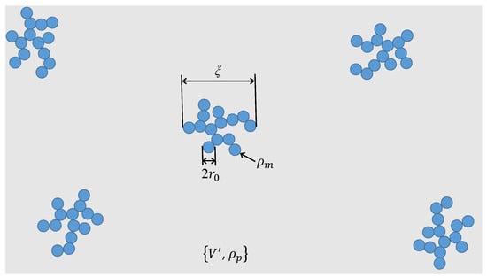
Figure 2.
(Color online) Schematic representation of the sample’s structure investigated in this work. The irradiated macroscopic volume (gray region) consists from a matrix with SLD in which are dispersed fractals with SLD , overall size , and size of the basic objects . The orientations and positions of the fractals are uncorrelated. Their number is enough large such that an observable signal is recorded at detector, and enough small such that the distances between fractals are larger than their overall size .
2.2.5. Polydispersity
In physical systems, the fractals usually have different sizes. We consider here that all fractals have the same shape while their size are distributed according to a distribution function defined such that gives the probability of finding an object whose size falls within . Without losing generality, throughout this paper it will be used the log-normal distribution function:
where is the variance and is the mean value of the length, is the relative variance, and . Therefore, by averaging Equation (27) over the distribution function (37), one obtains [71]:
where is the fractal volume. Analytic expressions for the form factor of each type of deterministic fractals shall be provided thereafter in their corresponding section. In the limit of strong polydispersity, i.e., when , the maxima and minima present in the scattering intensity of a deterministic fractal are completely smoothed and thus the intensities form random fractals can be modeled by using deterministic fractals with a high degree of size polydispersity.
Other important properties which will be used in calculating the SAS intensity are:
- when the length is scaled as ,
- when the particle is translated ,
- , when the particle consists of two non-overlapping subsets I and .
Certainly, for 2D models, all the volumes shall be replaced by the corresponding areas.
2.3. Monte Carlo Simulations
A Monte Carlo-based algorithm similar to the one described in Ref. [75] is used to generate the pddf . To this aim, the area occupied by a given fractal is filled with a large number of randomly generated points pairs , and all the distances between them are collected into a histogram with about M = 250 boxes. Such a histogram gives directly the function pddf: . Here, the coefficient C ensures that the form factor is normalized such that . Then, for arbitrarily values of the scattering vector q, the form factor is calculated by performing numerically the Fourier transform in Equation (31). The simulated scattering curves are used to validate the analytic expressions for the form factors.
Figure 3 illustrates the results of the above steps for a simple example of a disk of radius a. At the first step, the square which circumscribe the disk is approximated by a set of random points (upper left part). Those found inside the disk are kept (blue points) and the others (gray points) are eliminated. The upper-right part of the same figure shows the corresponding pddf, while the lower part shows the corresponding scattering intensity obtained from Equation (31) (red curve). For comparison, the same figure shows the analytic curve (black) of an infinite thin circular disk of the same size, and with a known expression of the form factor given by [76]:
where is the Bessel function of the first kind and the first order.
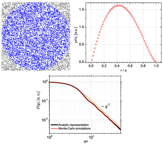
Figure 3.
(Color online) Upper left: Approximating a disk of radius a with a set of randomly distributed points (blue). Upper-right: the corresponding pddf . Lower part: A comparison between the analytic expression (black curve) and Monte Carlo simulations (red curve) of SAS intensities.
The results show an excellent agreement between the two curves in almost the whole q-range. However, small deviations begin to arise at large values of q () and are due to the intrinsic property of Monte Carlo method to approximate the disk by a finite collection of random points. The approximation can be improved by increasing the number of scattering points.
3. Small-Angle Scattering from Fractals
In this section, analytic forms of scattering intensity shall be derived for various types of fractals, by providing and deriving explicit expressions for the form, and respectively the structure factor appearing in Equation (26). For simplicity, the fractals considered here consist either from disks or from balls, but any other geometric form can be used. While in the former case the form factor is given by Equation (39), in the later one, the form factor of a ball of radius a can be written as [71]:
3.1. Random Mass Fractals
To derive the scattering structure factor of a mass fractal, let us choose first an imaginary sphere centered on the fractal and consider a spherical layer of radius r and width . Then, the number of balls (particles) within the spherical layer is:
where is the layer volume. Thus, the total number of particles within the sphere is given by: [39]. By differentiating Equation (5) and comparing with Equation (41), one obtains [39]:
where (see Figure 2).
This expression shows that for large values of r, since the fractal dimension is . However, any sample is characterized by a macroscopic density at large scale. Thus, in order to describe the large-scale behavior of , an exponential term of the form , known as the cutoff function is introduced [77]. Here, is the fractal outer cutoff, and it gives the distance above which the mass distribution is no longer described by the mass fractal law, and thus it coincides with the fractal size, as pointed out in Section 1. This cutoff function is faster than any power law, and it is clear that the larger the value of , the sharper the cutoff. In the reciprocal space, an increase of leads to the formation of a distinct jump just beyond the Guinier regime [77]. After this hump, the power-law decay (see Equation (47)) is still visible but at different levels, depending on the values of , and “ripples” occur for [77]. One of the most common cutoff functions, which provides a reasonable assumption for describing the behavior of at large distances, corresponds to , and this value will be used in the following. With the introduction of the exponential cutoff, a uniform density shall be subtracted, to avoid the divergence of the structure factor, and therefore we have [39]:
By introducing Equation (43) into Equation (28), one can write:
where is the gamma function. Depending on the values of the scattering vector q, we distinguish several main regions in the scattering intensity in Equation (31), with the structure factor given by Equation (44) and form factor by Equation (40):
- When ,and therefore the scattering intensity is dominated by . By comparing this with Equation (34) one can see that the outer cutoff is related to the mass fractal radius of gyration by [39]: .
- When ,and therefore still dominates in Equation (34) since yet . The last equation shows that the scattering intensity of a mass fractal is a straight line on a double logarithmic scale. Therefore, deviations from this line at low and values of the scattering vector q provide information about the fractal overall size , and respectively about the radius a of fractal basic unit.
- When ,and thus, for , , while dominates in the scattering intensity [73]. Therefore, scattering at large q values provides information about the fractal basic particles.
As an application of the above results, let us consider a two-dimensional (2D) DLA cluster, as a representative example of random mass fractals. The DLA is generated by particles undergoing a random walk due to Brownian motion, and which cluster into aggregates [78]. It is widely used to describe structures in which diffusion is the main means of transport, and it occurs often in dielectric breakdown, electrodeposition or Hele-Shaw flow.
The overall size of the generated DLA is nm and consists from particles of radius nm (Figure 4—upper row). The numerical values were chosen such that they fit into a typical range covered by SAS measurements. The corresponding pddf is shown in Figure 4—lower row (left; black points). For comparison, the pddf of an equivalent disk, i.e., a disk centered on the cluster and with radius is also shown (red points). The total number of distances used in calculating each pddf is about . When the positions of the disks forming the DLA and their shape are known, the calculations can be greatly simplified if one uses only the mass-center coordinates, since the number of points used in calculating the pddf is much lower. The corresponding Fourier transform will give the structure factor describing the relative positions of the disk inside the aggregate. By multiplying it with the disk form factor, the scattering intensity (Equation (31)) is recovered.
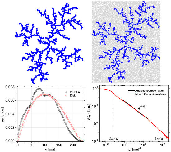
Figure 4.
(Color online) Upper row: Left—2D DLA cluster of overall size nm consisting from about 500 particles of radius nm, Right—the corresponding approximation with a set of randomly distributed points (blue). Lower row: Left—pddf of the 2D DLA (black points) and of an equivalent disk (red; see text for additional explanations), Right—A comparison between the analytic expression of SAS intensity (black curve) with Monte Carlo simulations (red curve).
The results show that in the case of DLA, although the pddf has an overall similar behavior as for the disk, it is characterized by the presence of local minima and maxima, with the main maxima (at nm) shifted to the left. These reflects deviations of the DLA from the circular symmetry of the disk. Also, the height of the maxima increases, and indicates the number of most common distances within DLA. This peak is followed by a second one, slightly shifted to the left (at nm), and less pronounced, and which partially follows the disk’s pddf for nm. This indicates that within this range the number of distances within DLA and the disk coincide. Finally, for nm the number of distances within DLA decreases faster, and both reach the same maximum value at nm. Please note that at nm the DLA’s pddf is quite flat in this region, and may pose difficulties in an accurate determination of overall size from SAS data, due to experimental errors [79].
Figure 4 lower row right shows the SAS intensity (red curve) from DLA obtained by Fourier transform (Equation (31)) of the corresponding pddf. The analytic expression (Equation (47)) is also shown in the fractal region (black curve). The results show a very good agreement between the two curves. The scattering exponent is 1.66 and coincides with the analytic value from mean-field theory for diffusion-limited cluster formation with [80] and with other computer simulations of Witten-Sander aggregates [81].
3.2. Random Surface Fractals
To derive the scattering law for surface fractals, one considers a system consisting from a random distribution of material with constant SLD . By denoting with c the fraction of the volume occupied by the material, then denotes the fraction of unoccupied volume, and the average density of the sample can be expressed as . Therefore, the density fluctuations can be expressed as:
and the mean square volume is:
Thus, Equation (25) becomes:
where the correlation function is defined by [38]:
The function represents the probability that if a point is in the occupied volume, then a second point situated at a distance r apart from the second point, belongs also to the occupied volume. Thus, from definition, excepting those points found at distance r apart from the pore boundary. In the latter case, the volume of the layer with occupied regions is , while in the former case, the volume is . Also, it is known that in the limit , the function is given by [38]:
and therefore, by using Equation (52), the correlation function becomes [38]:
Performing two integration by parts in Equation (51) and taking into account that both and its derivative tend to zero at large r, the scattering intensity can be rewritten as [38]:
Then, according to Erdélyi’s theorem for asymptotic expansion of Fourier integrals, in the limit of large values of the scattering vector q, the intensity becomes:
Finally, by using the correlation function given by Equation (54), the scattering intensity can be rewritten as:
which shows that for a surface fractal [38]:
A similar procedure can be used to show that for , . Therefore the scaling law is recovered, and taking into account that for surface fractals discussed here, the scattering intensity in Equation (1) is recovered. Please note that when , Equation (57) reduces to Porod law, where , and the density profile varies sharply over distances smaller than .
Since , the function in Equation (53) gives the probability that a point at distance r in an arbitrarily direction from a given point inside the fractal will itself be in the fractal. This holds true since there is only a small probability of finding an occupied point outside a particular fractal in which the origin is chosen. As such, c is negligible and thus , Therefore, , where represents now the correlation function of the fractal, and not of the whole sample, as in Equation (25). Therefore, Equation (51) gives:
with the SLD factor included in Equation (26). Thus, by using the property that , Equation (31) is recovered.
To illustrate the above results, we consider in the following a random surface fractal model which consists from disks whose radii follow a power-law distribution. The model is shown in Figure 5 upper left row, where disks with identical radii have the same color. Specifically, one considers that the radius of the largest disk (blue), also known as the zero-th fractal iteration () is , and the scaling factor . Then, the radius of the disks forming the first fractal iteration (green disks) is , the radius of the disks forming the second fractal iteration (black disks) is , and so on. From the construction one can see that each disk is tangent to at least another disk and they form an aggregate, of overall size nm. Since the number of disks at a given iteration increases by a factor of 3, then the fractal dimension of the model is , and therefore in the fractal region the corresponding form factor is given by (see discussion below Equation (58)):
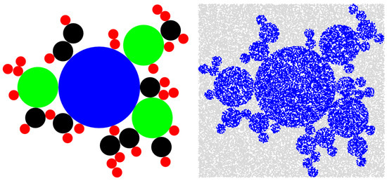
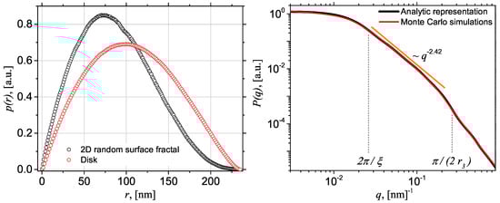
Figure 5.
(Color online) Upper row: Left—random surface fractal of overall size nm consisting from disks of different radii, Right—the corresponding approximation with a set of randomly distributed points (blue). Lower row: Left—pddf of the random surface fractal (black points) and of an equivalent disk (red), Right—A comparison between the analytic expression (black curve) of SAS intensity (Equation (34)) and Monte Carlo simulations (red curve).
Figure 5 upper-right row shows the discretized version of the surface fractal model used for computing the pddf in Figure 5 lower-left row (black). For comparison, the pddf of a disk of equivalent radius is also shown in red. The total number of distances used in both cases is about 1.54 ×. The results show that the pddf of the random surface fractal has a similar behavior as of the pddf of DLA (see Figure 4 lower-left row) in the sense that the main maximum is shifted to the left with respect to the disk’s maxima, while its height increases. Thus, this reflects the asymmetry of the model as compared to the circular one. However, as opposed to the pddf of DLA, for surface fractals the maxima are much less pronounced, and generally the curve is smoother. This indicates a more uniform structure of the surface fractal, which arise from the existence of disks of different sizes.
For surface fractals, it has been recently shown that the scattering intensity can be obtained by neglecting the spatial correlations between disks, and therefore one can use the approximation of independent units, i.e., [60]:
where , and is given by Equation (39). The corresponding intensity is shown in Figure 5 lower-right row (black), where one can see that the scattering exponent is in excellent agreement with the analytic value obtained above. The Monte Carlo simulations (red curve) are also in very good agreement with the theoretical results. This is to be expected, since there is an excellent agreement between theoretical and Monte Carlo-based curves of a disk (see Figure 3 lower row), while Equation (61) is just a sum of SAS intensities of disks of various radii. The edges of the fractal region are marked in Figure 5 lower row right by dotted vertical lines, and they provide information about the overall fractal size, and about the size of the smallest disk composing the fractal.
3.3. Deterministic Mass Factals
In the following, the scattering properties from deterministic mass fractals are illustrated on fractals similar to the well-known Cantor fractal. For this purpose, one considers first a square with edge which circumscribes a disk of radius such that their centers coincide. One also considers a Cartesian system of coordinates whose origin lies in the square center, and with axes parallel to the square edges. At first iteration, the disk of radius is replaced by 5 smaller disks of radius , with . One disk is situated in the origin, while the centers of the other disks are shifted from the origin by:
with all combinations of the signs, and . The second iteration is obtained by performing a similar operation on each of the 5 disks of radius , and so on. The “cross” mass fractal is obtained in the limit of infinite number of iterations. Figure 6 upper row shows the construction at iterations and 3, while in the middle row is shown the discretized version, for the same iterations. The total number of disks at m-th iteration is , and the radius of each disk is . Therefore, in accordance with Equation (5), the fractal dimension is given by:
and the total area of the fractal at m-th iteration is , where is the surface area of the disk at .
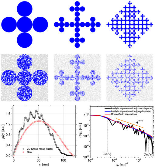
Figure 6.
(Color online) Upper row: Iterations and 3 of the deterministic “Cross” mass fractal of overall size nm. Middle row: the corresponding approximation with a set of randomly distributed points (blue). Lower row: Left—pddf of the “Cross” mass fractal (black points) and of an equivalent disk (red points), Right—A comparison between the mono- and polydisperse analytic expression (black, and respectively blue curve) of SAS intensity given by Equation (26) with the form factor given by Equation (65), and Monte Carlo simulations (red curve). The polydisperse curve is calculated with Equation (38), and the relative variance used is .
The position of the disk centers inside the fractal can be written as:
where , and . Then, for arbitrarily iteration number , the fractal form factor is given by:
The pddf of the cross-mass fractal at iteration , overall dimension nm, is shown in Figure 6 lower row left (black). For comparison, the pddf of the equivalent disk is shown also (red). The main feature of fractal’s pddf is the presence of a succession of local maxima and minima on a parabola-like function similar to that of the disk, but with the maximum shifted to smaller values of r. These features reflect both the deviations from the circular symmetry of the fractal, as well as its particular feature, in which a periodic structure arise in its construction. Please note that at nm the fractal’s pddf is almost flat, thus making it difficult to estimate its overall dimension from SAS data.
The fractal form factor at obtained from the Fourier transform of the pddf is shown in Figure 6 lower row right in black, while the scattering curve obtained from Monte Carlo simulations is shown in red. The analytic curve is characterized by the presence of the three main regions: Guinier, at , fractal, at , where is the radius of the disk at iteration , and Porod, at . In the fractal region, the scattering curve consists from a superposition of maxima and minima on a power-law decay. This is known in the literature as a generalized power-law decays (see also Introduction section). The exponent of the power-law decay is approximately 1.46, which is agreement with the analytic value given by Equation (63). The number of main minima in the fractal region is equal to 3, and it coincides with the fractal iteration number. The periodicity of these minima on a double logarithmic scale is , and it can be used to extract information about the fractal scaling factor. By knowing the fractal dimension , iteration number m and the scaling factor , the number of disks composing the mass fractal can be determined from the relation [58]. When measurements are performed on an absolute scale, the Porod region can be used to extract the ratio , where is the total perimeter of the fractal at m-th iteration, and is the total surface area (see above). For 3D fractals this would give the specific surface , where is the fractal volume at m-th iteration.
The corresponding polydisperse curve (blue) is calculated by using Equation (37), where the relative variance is . In this case, the simple power-law decay, specific to scattering from random mass fractals (see Figure 4) is recovered, and the scattering exponent is preserved. Please note that generally, the oscillations in the fractal region are still visible up to , and thus the polydisperse curve can be used to extract the fractal iteration number and scaling factor, as discussed before for the monodisperse case. This is important from an experimental point of view, since in practice it is very hard to prepare samples containing perfectly monodisperse fractals.
The Monte Carlo simulations (red) show a good agreement with the polydisperse curve, excepting the presence, in the former case, of a local bump at nm, and of slight deviations at q close to the end of the fractal region. This agreement is to be expected, since the behavior of SAS intensity in the fractal region is dominated by the relative positions of the disks inside the fractal, as described by the generative function given by Equation (64). This implies that one can calculate the intensity based only on the center-of-mass positions of each disk [58]. Then, each of the most pronounced maxima and minima in the fractal region corresponds to the interference cluster amplitude, where each cluster represents a fractal iteration. The positions and amplitudes of these maxima and minima are related to the most common distances between the center-of-masses [58]. However, when the scattering intensity is calculated by using randomly generated points, we use only an approximation of the fractal shape and not the distances between center-of-masses. As such, the number of possible distances used is much higher, and thus the maxima and minima are significantly smeared out. As described above, the polydispersity also leads to smearing the maxima and minima. Thus, although the effects on the scattering curve are similar, their nature is different.
Please note that in building the cross-mass fractal, a single scaling factor has been used at each iteration, while the ratio between the size of the disks to the distances between them is about unity. By releasing these constraints, additional fractal classes, each one with its own “signature” on the scattering curve, can be investigated. In particular, by increasing the value of the scaling factor after a predefined number of iterations (every second, every third, etc.), one obtains a fractal with positive Lebesgue measure (also known as fat fractals). It has been recently shown that for fat fractals, the scattering curve consists from a succession of power-law decays with increasing values of the scattering exponents [59]. Such models can be used to describe the properties of hierarchically structured materials in which the fractal dimension varies with the scale (iterations with constant scaling factor). However, within each scale, the scattering behavior of regular (thin) fractals is recovered (Figure 4). Also, allowing the distances between disks to be much bigger than the disk’s size, induces the appearance of a constant region (also known as a plateau or asymptotic) between the fractal and Porod regions [60]. Therefore, the beginning and the end of this plateau can be used to estimate the length of the minimal distances between disks, and respectively their size.
3.4. Deterministic Surface Fractals
The construction process of the deterministic surface is similar to that of the cross-mass fractal, where an initial disk is repeatedly divided into a set of smaller structures, according to the same rule for each iteration. If we denote by the radius of the disk at (initiator), then at the first iteration (; generator), there are also four disks of radius whose centers are situated on the positive and negative coordinate axes, at a distance from the origin. At the m-th approximation, the surface fractal is built from the -th approximation by adding disks of radii placed at a distance from the centers of the disks of radii , in all directions of the coordinate axes and on the positions that are already not occupied by other disks (Figure 7 upper row).
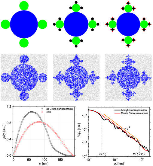
Figure 7.
(Color online) Upper row: Iterations and 3 of the deterministic “Cross” surface fractal of overall size nm (at ). Middle row: the corresponding approximation with a set of randomly distributed points (blue). Lower row: Left—pddf of the random surface fractal (black points) and of an equivalent disk (red points), Right—A comparison between the approximation of independent units (black curve) of SAS intensity (Equation (61)) and Monte Carlo simulations (red curve).
At m-th iteration, the obtained Cross-surface fractal is built as a sum of mass fractals at iterations n from 0 to m. In Figure 7 upper row, each mass fractal is colored differently, and thus at the surface fractal consists from mass fractals at iterations . By construction, one can see that at m-th iteration, the overall size of the surface fractal is very well approximated by the overall size of the mass fractal at iteration . Please note that from the point of view of scattering properties, the main difference between cross-mass and surface fractals is that the former ones consist from disks of the same size, while the later ones consist from disks of different sizes, following a power-law distribution. Their number is given by:
and their radii are distributed in the following way: one disk of radius (blue), 4 disks of radius (green), 12 disks of radius (black), and so on. Since at m-th iteration the radius is , then the surface fractal dimension is:
The discrete version of the surface fractal is shown in Figure 7 middle row, and the corresponding pddf at is shown in Figure 7 lower-low left (black). For comparison, the pddf of the equivalent disk is also shown (red). The figure clearly shows that the pddf of the surface fractal is much smoother than the pddf of the cross-mass fractal (Figure 6 lower row left). This is due to the presence of disks of various sizes in th former case. However, the overall behavior is similar to the one of mass fractal where the main maximum is shifted to the left of disk’s maximum, while at large r, the pddf is almost completely flat. These features reflect the deviations from the circular symmetry, and which are specific to the surface fractal model.
Since the cross-surface fractal consists from a superposition of mass fractals at various iterations, by adding their amplitudes and normalizing the result to unity at , one can write [60]:
with , and where is the mass fractal form factor at n-th iteration. Therefore, the surface fractal form factor can be written as:
where , and is the total surface area of the fractal at m-th iteration.
Please note that in some cases it is very difficult to derive an analytic expression for the mass fractal form factor in Equation (69). However, if we are not interested in the intricate behavior of the scattering curve, one can use the approximation of independent units (AIU) in Equation (61) to calculate the scattering intensity of surface fractals. Here, this approach is used, and the results are shown in Figure 7 lower row right (black). It is clear that in the fractal region i.e., for , the scattering intensity decays proportional to . Thus, the fractal dimension of the surface fractal is , as predicted by Equation (67). Despite using the AIU, in the fractal range one can observe the presence of three pronounced minima at nm. This shows that the surface fractal consists from three iterations of mass fractals. The minima positions also show an approximate log-periodicity with the scale factor . The results are similar to those of scattering from deterministic cross-mass fractals, but the nature of the log-periodicity is different. While in the case of scattering from mass fractals, the periodicity arises from the self-similarity of distances between disks, for surface fractals, it arises from the self-similarity of disk sizes.
Monte Carlo simulations are presented in the same figure (red), and show that the scattering exponent in the fractal region of the scattering curve is recovered, but without following in detail the small oscillations present in the analytic curve. This effect is similar to the one seen in Figure 6 lower row right for mass fractals, and arise due to the discretization of the surface fractal with randomly positioned points.
3.5. Deterministic Multifractals
Single-scale fractal presented so far, lead to homogeneous structures and are the simplest cases of fractal systems. An exception is the fat fractal discussed in Section 3.3, which although have different scaling factors, they occur at different scales. However, real fractal may have far more reach scaling and self-similar properties that change from point to point. They are known as multifractals, and to model their scattering properties, one should consider structures in which various scaling factors occurs at the same scale.
For simplicity, we consider in the following a multifractal built from two scaling factors and . The initiator () is a single disk, while the first iteration () consists from four disks found on the coordinate axes, as in the case of deterministic cross-mass and surface fractals (see Figure 6 and Figure 7 upper rows), each one with the scaling factor , and one disk in the center, with the scaling factor . The second iteration is obtained by repeating the same procedure for each of the five disks at , and so on. It is clear that when , one recovers the single-scale deterministic cross-mass fractal shown in Figure 6 upper row.
Figure 8 upper row shows the cross multifractal models at iteration for and (model MI, left), and (model MII, middle) and and (model MIII, right). In this figure, the disks with the same radius have the same color. Note that although for model MIII, the scaling factors are different, they are very close to each other, thus leading to disks of similar radii. Consequently, they all have the same color. The fractal dimension of each model is calculated according to Equation (8), with and . Therefore, one obtains for model MI, for model MII and for model MIII. The total number of particles at m-th iteration is , and the total surface area is , where is the surface area of the single disk at .
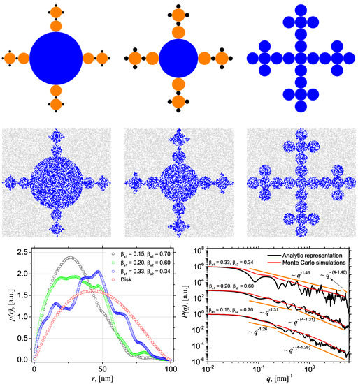
Figure 8.
(Color online) Upper row: The second iteration () of the deterministic “Cross” multifractal of overall size nm at various scaling factors: Left—Model MI ( and ), Middle—Model MII ( and ), Right—Model MIII ( and ). For each fractal, the disks of the same radius have the same color. Middle row: the corresponding approximation with a set of randomly distributed points (blue). Lower row: Left—pddf of the multifractal models and of an equivalent disk (red points), Right—A comparison between the analytic expression (black curve) of SAS intensity (Equation (70)) and Monte Carlo simulations (red curve). The curves for models MII and MIII are shifted vertically by a factor of , and respectively of , for clarity.
Therefore, the multifractal form factor can be expressed through a recurrence relation between subsequent iterations. For an arbitrarily two-scale multifractal, one can write [62,82]:
where the generative function is given by Equation (64), , and the form factor at is given by Equation (39). Please note that the choice of the generative functions, of the initial shape, of the number of disks and their positions is arbitrarily. Thus, Equation (70) gives the form factor of a two-scale multifractal at an arbitrarily iteration m.
Figure 8 middle row shows the discretized version of the cross multifractals used to calculate the pddf (Figure 8 lower row left) of models MI (black), model MII (green) and model MIII (blue) with the overall size nm. For comparison, the pddf of the equivalent disk is also shown (red). The most pronounced differences, as compared to the disk’s pddf occur in model MI, where the maxima is the left-most shifted and has the highest values. This shows that the structure corresponding to model MI is the most heterogeneous. This can be clearly seen also from their construction: while the model MI consists from disks with the highest difference in the values of their radii, for model MIII (i.e., for a single-scale fractal), the structure consists from disks of similar radii, and is more homogeneous. In addition, the local maxima and minima present in the pddf reflect the relative values of various distances within the fractal. In particular, the main maximum at nm (model MI), nm (model MII), and nm (model MIII) give the most common distances inside the multifractal.
Figure 8 lower row right shows the SAS curves of the three models at iteration , calculated using Equation (70). The main feature of the curve is the presence of the three main regions: Guinier, fractal and Porod (not shown here) as in the case of deterministic mass and surface fractals, and which allows extraction of the main structural information. However, a specific feature of scattering from multifractals is the appearance of an additional surface fractal region between the mass fractal and Porod regions. In the mass fractal region, the scattering exponent coincides with the mass fractal dimension , while in the surface fractal region, the exponent is . This shows that the multifractal model consists from mass fractals in which the basic units are not simply Euclidean objects, but they are themselves complex structures, in particular surface fractals, which in their turn have disks as basic units. Please note that while the overall length of the two mass and surface fractal regions is defined by the overall fractal size, and respectively by the two scaling factors, i.e., , the length of each individual region depends on the value of , i.e., the higher the value of the longer the mass fractal region and the shorter the surface fractal region.
Monte Carlo simulations performed on all three models at are also presented in Figure 8 lower row right (red). The results confirm the values of the scattering exponents in both regions. However, the fine structure of the scattering curve is lost in the simulated curves, for the same reason as in the case of deterministic mass and surface fractals. Therefore, experimental SAS data showing a succession of mass-to-surface fractal regions, can be attributed to multifractal (i.e., heterogeneous) structures. Thus, the procedure of extracting structural information about multifractals involves a separate analysis of both the mass, and respectively the surface fractal regions (Section 3.3 and Section 3.4).
4. Conclusions
The latest advances in preparation of complex materials allow the synthesis of various types of nanomaterials based on deterministic fractals. These materials have improved physical properties such as optical, electronic, mechanical thermal ones, with important applications in surface engineering, heterogeneous catalysis, manufacturing of cloaking devices etc. It is already known that generally, the main reason for the improved properties is the exact self-similar structure of the fractal. Therefore, one of the fundamental challenges is to establish the correlations between their physical and chemical properties from one side, and the structural properties from another one. While the evolution of their properties can be assessed by complex quantum mechanical models, the nanoscale structure is generally addressed by using the SAS technique. In the latter case, one of the main reasons for using SAS is that it provides statistically significant quantities averaged over a macroscopic volume, it allows for sample deuteration (when neutrons are used) and eliminates the requirement of sample preparation, specific to other structural methods.
Here, the main structural properties of deterministic fractals are determined based on information provided by SAS technique. The focus is on differentiating between various classes of fractal, by using information from the corresponding scattering curves. For this purpose, several new theoretical models are introduced, and their scattering properties are validated against data based on Monte Carlo simulations. Table 1 summarizes the structural parameters which can be obtained from SAS curves for the main classes of fractals. Please note that in Table 1 are listed only those properties specific to each class of fractals. Besides them, by using SAS one can obtain also additional properties that are not necessarily related to a specific fractal, such as the: overall size, specific surface, molecular weight, size of the basic unit, correlation/persistence length, or the mass per unit length.

Table 1.
Fractal specific parameters which can be obtained from a SAS experiment. Here and are the mass, and respectively the surface fractal dimension, is the mass and surface fractals scaling factor, m is the mass fractal iteration number, , , and are the scaling factors, the number of basic units, iteration number and respectively the fractal dimensions at i-th structural level () in a fat fractal, and , with are the multifractal scaling factors, is the number of basic units in a mass fractal, h is the characteristic minimal distance between basic units in a mass fractal, and , with l the size of basic units composing the mass fractal. The exponents of the scaling factors and number of units occurring for fat fractals denote an index (over the structural levels) and not a power.
Figure 9 shows schematically the scattering curves corresponding to the fractals listed in Table 1. Each of them is compared to the curve of random mass fractals (taken as a reference due to its widespread occurrence in experimental data). In this figure, the random mass fractals have been labeled differently, depending on the context, and in accordance with the most common terminology in the literature. As such, mass fractals, random fractals, monofractals and thin fractals, all represent a single-scale random mass fractal. A representative example is given by DLA, shown in Figure 4 upper row. The results in Figure 9 show that each class of fractals has its own imprint on the scattering curve, and thus, the SAS technique can differentiate between:
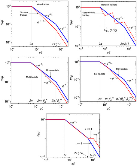
Figure 9.
(Color online) Schematic representation of SAS from different classes of 2D fractals Upper row: Left—mass and surface fractals, Right—random and deterministic fractals. Middle row: Left—mono and multifractals, Right—Thin and fat fractals. Lower row: and fractals (see below). Here is the overall size of mass fractals, and respectively the size of the largest disk in a surface fractal, (including and ) and are the mass and, respectively the surface fractal dimensions, l is the size of disks in a mass fractal, and respectively the size of smallest disk in a surface fractal, m (including and ) are the fractal iteration numbers, (including and ) are the scaling factors, h is the minimal distance between the disks, and .
- Mass and surface fractals (Figure 9 upper row, left). The differentiation is made through the value of the scattering exponent in the fractal region that is for random mass fractals, and for surface fractals. Here, d is the Euclidean dimension of the space in which the fractal is embedded.
- Random and deterministic fractals (Figure 9 upper row, right). The differentiation is made based on the type of power-law decay, i.e., a simple power-law decay for random fractals, and a generalized power-law decay (a complex superposition of minima and maxima on a simple power-law decay) for deterministic fractals.
- Mono and multifractals (Figure 9 middle row, left). The differentiation is made through the presence of one or more power-decays, either simple or generalized. For monofractals, there is a single power-law decay, while for two-scale multifractals, there is a succession of a mass fractal followed by a surface fractal. When the two scaling factors have similar values, the length of the surface fractal region is very short, and vice-versa.
- Thin and fat fractals (Figure 9 middle row, right). The differentiation is made in a similar way as in the previous case. However, the main difference is that the surface fractal region is replaced by another mass fractal region with the exponent smaller than the one of the first mass fractal region.
- and fractals (Figure 9 lower row). The differentiation is made through the presence of an additional region of constant intensity between the fractal and Porod regions. For fractal in which the ratio of the size of basic units to the minimal characteristic distances between them is about unity, the length of this constant region is very short. However, for fractals with , the length of the constant region is much bigger.
Most of the above results illustrated here, are validated by Monte Carlo simulations. Although they represent important advances in structural analysis of fractal structures, there are still important open question which need to be addressed.
Experimentally, the main issues arise from the loss of information about phases, the influence of instrumental limitations, polydispersity and of incoherent scattering at high q, which may hinder the extraction of structural parameters from a SAS curve. The loss of phase information is an intrinsic drawback of the SAS method, since it gives the absolute value of the Fourier transform of the density. In the case of randomly oriented fractals, the square of the Fourier transform is also averaged over all possible orientations of vector . This operation leads to an ill-posed problem in recovering the density from SAS data. Such issue can be handled by measuring the scattering of an ensemble of aligned fractals from different angles with a position sensitive detector. The instrumental limitations arise from the finite resolution of the collimation and detection systems, as well as from the wavelength spread. For samples based on deterministic fractals, these lead to either partial or a total smearing of the scattering curves, and the fine structure of the intensity is lost. In the former case, the main maxima and minima are still visible, and all the structural parameters presented in Table 1 can be recovered. However, in the latter case, all the maxima and minima are completely smeared out. This leads to the impossibility of extracting the scaling factor(s) and the iteration number. The effect of polydispersity is similar to the one of finite instrumental resolution, i.e., the higher the polydispersity, the more smeared the SAS curve. Finally, the q-independent background of SAS curve, determined by the scattering density of irradiated nuclei with nonzero spins such as or isotopes, may hinder the structural features arising at high q. In this case, one can use deuteration to increase the contrast and reduce the background.
Theoretically, since a given fractal dimension may represent virtually an infinite number of structures, then how one can differentiate between them? Second, multifractals are characterized by a whole spectrum of dimensions given by Equations (11) or (12). Can SAS, eventually in combination with other methods, provide other dimensions, besides (see Equation (13))? And if the multifractal consists from more than two scaling factors, which is probably one of the most common situations in physical samples, can we recover all the scaling factor from SAS curves?
From a practical point of view, partial answers to these questions begin to emerge. The progress in SAS instrumentation could eliminate the disadvantage of finite instrumental resolution, to a sufficiently high degree, without sacrificing the complex morphology of deterministic fractals and without increasing the measurement time. Similarly, recent advances in nanotechnology, materials science and chemistry allows preparation of highly monodisperse samples. Of particular importance is the use of ptychographic methods for phase recovery in coherent SAS by numerical procedures. Also, a combined use of SAXS with tensor tomography, also known as 3D scanning SAXS, allows determination of 3D orientation of nanofractals in a bulk specimen, and thus symmetries within the sample can be exploited to extract additional structural information about fractals.
Funding
This research received no external funding.
Conflicts of Interest
The author declares no conflict of interest.
References
- Chaudhuri, B.; Muñoz, I.G.; Qian, S.; Urban, V.S. (Eds.) Biological Small Angle Scattering: Techniques, Strategies and Tips, 1st ed.; Springer: Singapore, 2017; Volume 1009, p. 268. [Google Scholar] [CrossRef]
- Glatter, O. Scattering Methods and Their Application in Colloid And Interface Science, 1st ed.; Elsevier: Amsterdam, The Netherlands, 2018; p. 404. [Google Scholar]
- Jaksch, S.; Gutberlet, T.; Müller-Buschbaum, P. Grazing-incidence scattering—Status and perspectives in soft matter and biophysics. Curr. Opin. Colloid Interface Sci. 2019, 42, 73–86. [Google Scholar] [CrossRef]
- Allen, A.J. Scattering methods for disordered heterogeneous materials. In International Tables for Crystallography Volume H: Powder Diffraction; Gilmore, C.J., Kaduk, J.A., Schnek, H., Eds.; Wiley: Hoboken, NJ, USA, 2019; Chapter 5.8; pp. 673–696. [Google Scholar] [CrossRef]
- Wittmeier, A.; Cassini, C.; Hemonnot, C.; Weinhausen, B.; Bernhardt, M.; Salditt, T.; Koster, S. Scanning Small-Angle-X-Ray Scattering for Imaging Biological Cells. Microsc. Microanal. 2018, 24, 336–339. [Google Scholar] [CrossRef][Green Version]
- Mühlbauer, S.; Honecker, D.; Périgo, E.A.; Bergner, F.; Disch, S.; Heinemann, A.; Erokhin, S.; Berkov, D.; Leighton, C.; Eskildsen, M.R.; et al. Magnetic small-angle neutron scattering. Rev. Mod. Phys. 2019, 91, 015004. [Google Scholar] [CrossRef]
- Mahieu, E.; Gabel, F.; IUCr. Biological small-angle neutron scattering: Recent results and development. Acta Cryst. D 2018, 74, 715–726. [Google Scholar] [CrossRef]
- Oliver, R.C.; Rolband, L.A.; Hutchinson-Lundy, A.M.; Afonin, K.A.; Krueger, J.K. Small-Angle Scattering as a Structural Probe for Nucleic Acid Nanoparticles (NANPs) in a Dynamic Solution Environment. Nanomaterials 2019, 9, 681. [Google Scholar] [CrossRef]
- Kryukova, A.E.; Shpichka, A.I.; Konarev, P.V.; Volkov, V.V.; Timashev, P.S.; Asadchikov, V.E. Shape Determination of Bovine Fibrinogen in Solution Using Small-Angle Scattering Data. Cryst. Rep. 2018, 63, 871–873. [Google Scholar] [CrossRef]
- Palit, S.; He, L.; Hamilton, W.A.; Yethiraj, A.; Yethiraj, A. Combining Diffusion NMR and Small-Angle Neutron Scattering Enables Precise Measurements of Polymer Chain Compression in a Crowded Environment. Phys. Rev. Lett. 2017, 118, 097801. [Google Scholar] [CrossRef]
- Sakurai, S. Recent developments in polymer applications of synchrotron small-angle X-ray scattering. Polym. Int. 2017, 66, 237–249. [Google Scholar] [CrossRef]
- Horkay, F.; Basser, P.J.; Hecht, A.M.; Geissler, E. Ionic effects in semi-dilute biopolymer solutions: A small angle scattering study. J. Chem. Phys. 2018, 149, 163312. [Google Scholar] [CrossRef]
- Mortensen, K.; Annaka, M. Stretching PEO–PPO Type of Star Block Copolymer Gels: Rheology and Small- Angle Scattering. ACS Macro Lett. 2018, 7, 1438–1442. [Google Scholar] [CrossRef]
- Bocz, K.; Decsov, K.E.; Farkas, A.; Vadas, D.; Bárány, T.; Wacha, A.; Bóta, A.; Marosi, G. Non-destructive characterisation of all-polypropylene composites using small angle X-ray scattering and polarized Raman spectroscopy. Compos. Part A 2018, 114, 250–257. [Google Scholar] [CrossRef]
- Wolff, M.; Saini, A.; Simonne, D.; Adlmann, F.; Nelson, A. Time Resolved Polarised Grazing Incidence Neutron Scattering from Composite Materials. Polymers 2019, 11, 445. [Google Scholar] [CrossRef] [PubMed]
- Bhaway, S.M.; Qiang, Z.; Xia, Y.; Xia, X.; Lee, B.; Yager, K.G.; Zhang, L.; Kisslinger, K.; Chen, Y.M.; Liu, K.; et al. Operando Grazing Incidence Small-Angle X-ray Scattering/X-ray Diffraction of Model Ordered Mesoporous Lithium-Ion Battery Anodes. ACS Nano 2017, 11, 1443–1454. [Google Scholar] [CrossRef] [PubMed]
- Wang, L.M.; Petracic, O.; Kentzinger, E.; Rücker, U.; Schmitz, M.; Wei, X.K.; Heggen, M.; Brückel, T. Strain and electric-field control of magnetism in supercrystalline iron oxide nanoparticle–BaTiO3 composites. Nanoscale 2017, 9, 12957–12962. [Google Scholar] [CrossRef] [PubMed]
- Choi, Y.; Paik, D.; Bogdanov, S.; Valiev, E.; Borisova, P.; Murashev, M.; Em, V.; Pirogov, A. Neutron scattering on humane compact bone. Phys. B 2018, 551, 218–221. [Google Scholar] [CrossRef]
- Busch, A.; Kampman, N.; Bertier, P.; Pipich, V.; Feoktystov, A.; Rother, G.; Harrington, J.; Leu, L.; Aertens, M.; Jacops, E. Predicting Effective Diffusion Coefficients in Mudrocks Using a Fractal Model and Small-Angle Neutron Scattering Measurements. Water Resour. Res. 2018, 54, 7076–7091. [Google Scholar] [CrossRef]
- Penttilä, P.A.; Rautkari, L.; Österberg, M.; Schweins, R. Small-angle scattering model for efficient characterization of wood nanostructure and moisture behaviour. J. Appl. Cryst. 2019, 52, 369–377. [Google Scholar] [CrossRef]
- Li, A.; He, R.; Bian, Z.; Song, H.; Chen, X.; Zhou, J. Enhanced lithium storage performance of hierarchical CuO nanomaterials with surface fractal characteristics. App. Surf. Sci. 2018, 443, 382–388. [Google Scholar] [CrossRef]
- Wang, Y.; Maurel, G.; Couty, M.; Detcheverry, F.; Merabia, S. Implicit Medium Model for Fractal Aggregate Polymer Nanocomposites: Linear Viscoelastic Properties. Macromolecules 2019, 52, 2021–2032. [Google Scholar] [CrossRef]
- Wei, R.; Wang, X.; Zhang, X.; Wang, S.; Zhu, S.; Du, S. A Novel Method for Manufacturing High-Performance Layered Silicate/Epoxy Nanocomposites Using an Epoxy-Diamine Adduct to Enhance Compatibility and Interfacial Reactivity. Macromol. Mater. Eng. 2018, 303, 1800065. [Google Scholar] [CrossRef]
- Yue, H.; Reguero, V.; Senokos, E.; Monreal-Bernal, A.; Mas, B.; Fernández-Blázquez, J.; Marcilla, R.; Vilatela, J. Fractal carbon nanotube fibers with mesoporous crystalline structure. Carbon 2017, 122, 47–53. [Google Scholar] [CrossRef]
- Zhang, J.; Li, H.; Ye, J.; Cao, Z.; Chen, J.; Kuang, Q.; Zheng, J.; Xie, Z. Sierpinski gasket-like Pt–Ag octahedral alloy nanocrystals with enhanced electrocatalytic activity and stability. Nano Energy 2019, 61, 397–403. [Google Scholar] [CrossRef]
- Mandelbrot, B.B. The Fractal Geometry of Nature; W.H. Freeman: New York, NY, USA, 1982; p. 460. [Google Scholar]
- Zhu, W.; Esteban, R.; Borisov, A.G.; Baumberg, J.J.; Nordlander, P.; Lezec, H.J.; Aizpurua, J.; Crozier, K.B. Quantum mechanical effects in plasmonic structures with subnanometre gaps. Nat. Commun. 2016, 7, 11495. [Google Scholar] [CrossRef] [PubMed]
- Sichert, J.A.; Tong, Y.; Mutz, N.; Vollmer, M.; Fischer, S.; Milowska, K.Z.; García Cortadella, R.; Nickel, B.; Cardenas-Daw, C.; Stolarczyk, J.K.; et al. Quantum Size Effect in Organometal Halide Perovskite Nanoplatelets. Nano Lett. 2015, 15, 6521–6527. [Google Scholar] [CrossRef]
- Nazmitdinov, R.G. From Chaos to Order in Mesoscopic Systems. Phys. Part. Nucl. Lett. 2019, 16, 159–169. [Google Scholar] [CrossRef]
- Schaefer, D.W.; Justice, R.S. How Nano Are Nanocomposites? Macromolecules 2007, 40, 8501–8517. [Google Scholar] [CrossRef]
- Yurekli, K.; Mitchell, C.A.; Krishnamoorti, R. Small-angle neutron scattering from surfactant-assisted aqueous dispersions of carbon nanotubes. J. Am. Chem. Soc. 2004, 126, 9902–9903. [Google Scholar] [CrossRef]
- Yin, W.; Dadmun, M. A New Model for the Morphology of P3HT/PCBM Organic Photovoltaics from Small-Angle Neutron Scattering: Rivers and Streams. ACS Nano 2011, 5, 4756–4768. [Google Scholar] [CrossRef]
- Stevens, D.A.; Dahn, J.R. An In Situ Small-Angle X-Ray Scattering Study of Sodium Insertion into a Nanoporous Carbon Anode Material within an Operating Electrochemical Cell. J. Electrochem. Soc. 2000, 147, 4428–4431. [Google Scholar] [CrossRef]
- Zabar, S.; Lesmes, U.; Katz, I.; Shimoni, E.; Bianco-Peled, H. Studying different dimensions of amylose-long chain fatty acid complexes: Molecular, nano and micro level characteristics. Food Hydrocoll. 2009, 23, 1918–1925. [Google Scholar] [CrossRef]
- Jacques, D.A.; Trewhella, J. Small-angle scattering for structural biology-Expanding the frontier while avoiding the pitfalls. Prot. Sci. 2010, 19, 642–657. [Google Scholar] [CrossRef] [PubMed]
- Li, T.; Senesi, A.J.; Lee, B. Small Angle X-Ray Scattering for Nanoparticle Research. Chem. Rev. 2016, 116, 11128–11180. [Google Scholar] [CrossRef] [PubMed]
- Pfeifer, P.; Ehrburger-Dolle, F.; Rieker, T.P.; González, M.T.; Hoffman, W.P.; Molina-Sabio, M.; Rodríguez-Reinoso, F.; Schmidt, P.W.; Voss, D.J. Nearly Space-Filling Fractal Networks of Carbon Nanopores. Phys. Rev. Lett. 2002. [Google Scholar] [CrossRef] [PubMed]
- Bale, H.D.; Schmidt, P.W. Small-Angle X-Ray-Scattering Investigation of Submicroscopic Porosity with Fractal Properties. Phys. Rev. Lett. 1984, 53, 596–599. [Google Scholar] [CrossRef]
- Teixeira, J. Small-angle scattering by fractal systems. J. Appl. Cryst. 1988, 21, 781–785. [Google Scholar] [CrossRef]
- Pfeifer, P. Simple Models for the Formation of Random Rough Surfaces. In Multiple Scattering of Waves in Random Media and Random Rough Surfaces, Proceedings of an International Symposium, University Park, PA, USA, 29 July–2 August 1985; Varadan, V.V., Varadan, V.K., Eds.; Pennsylvania State University State College: State College, PA, USA, 1987; p. 964. [Google Scholar]
- Martin, J.E.; Hurd, A.J. Scattering from fractals. J. Appl. Cryst. 1987, 20, 61–78. [Google Scholar] [CrossRef]
- Schmidt, P.W. Small-angle scattering studies of disordered, porous and fractal systems. J. Appl. Cryst. 1991, 24, 414–435. [Google Scholar] [CrossRef]
- Beaucage, G. Approximations Leading to a Unified Exponential/Power-Law Approach to Small-Angle Scattering. J. Appl. Cryst. 1995, 28, 717–728. [Google Scholar] [CrossRef]
- Beaucage, G. Small-Angle Scattering from Polymeric Mass Fractals of Arbitrary Mass-Fractal Dimension. J. Appl. Cryst. 1996, 29, 134–146. [Google Scholar] [CrossRef]
- Hammouda, B. A new Guinier–Porod model. J. Appl. Cryst. 2010, 43, 716–719. [Google Scholar] [CrossRef]
- Papagiannopoulos, A.; Meristoudi, A.; Pispas, S.; Keiderling, U. Thermal response of self-organization in an amphiphilic triblock polyelectrolyte and the influence of the globular protein lysozyme. Eur. Polym. J. 2018, 99, 49–57. [Google Scholar] [CrossRef]
- Anovitz, L.M.; Cole, D.R. Characterization and Analysis of Porosity and Pore Structures. Rev. Miner. Geochem. 2015, 80, 61–164. [Google Scholar] [CrossRef]
- Qiao, D.; Liu, H.; Yu, L.; Bao, X.; Simon, G.P.; Petinakis, E.; Chen, L. Preparation and characterization of slow- release fertilizer encapsulated by starch-based superabsorbent polymer. Carbohydr. Polym. 2016, 147, 146–154. [Google Scholar] [CrossRef] [PubMed]
- Liu, D.; Song, L.; Song, H.; Chen, J.; Tian, Q.; Chen, L.; Sun, L.; Lu, A.; Huang, C.; Sun, G. Correlation between mechanical properties and microscopic structures of an optimized silica fraction in silicone rubber. Compos. Sci. Technol. 2018, 165, 373–379. [Google Scholar] [CrossRef]
- Bauer, P.; Amenitsch, H.; Baumgartner, B.; Koberl, G.; Rentenberger, C.; Winkler, P.M. In-situ aerosol nanoparticle characterization by small angle X-ray scattering at ultra-low volume fraction. Nat. Commun. 2019, 10, 1122. [Google Scholar] [CrossRef] [PubMed]
- Song, P.; Tu, X.; Bai, L.; Sun, G.; Tian, Q.; Gong, J.; Zeng, G.; Chen, L.; Qiu, L. Contrast Variation Small Angle Neutron Scattering Investigation of Micro- and Nano-Sized TATB. Materials 2019, 12, 2606. [Google Scholar] [CrossRef] [PubMed]
- Shang, J.; Wang, Y.; Chen, M.; Dai, J.; Zhou, X.; Kuttner, J.; Hilt, G.; Shao, X.; Gottfried, J.M.; Wu, K. Assembling molecular Sierpiński triangle fractals. Nat. Chem. 2015, 7, 389–393. [Google Scholar] [CrossRef]
- Wang, L.; Liu, R.; Gu, J.; Song, B.; Wang, H.; Jiang, X.; Zhang, K.; Han, X.; Hao, X.Q.; Bai, S.; et al. Self-Assembly of Supramolecular Fractals from Generation 1 to 5. J. Am. Chem. Soc. 2018, 140, 14087–14096. [Google Scholar] [CrossRef]
- Wang, Y.; Xue, N.; Li, R.; Wu, T.; Li, N.; Hou, S.; Wang, Y. Construction and Properties of Sierpiński Triangular Fractals on Surfaces. Chem. Phys. Chem. 2019, 20, 2262–2270. [Google Scholar] [CrossRef]
- Newkome, G.R.; Moorefield, C.N. From 1 → 3 dendritic designs to fractal supramacromolecular constructs: Understanding the pathway to the Sierpiński gasket. Chem. Soc. Rev. 2015, 44, 3954–3967. [Google Scholar] [CrossRef]
- Malankowska, M.; Schlautmann, S.; Berenschot, E.; Tiggelaar, R.; Pina, M.; Mallada, R.; Tas, N.; Gardeniers, H. Three-Dimensional Fractal Geometry for Gas Permeation in Microchannels. Micromachines 2018, 9, 45. [Google Scholar] [CrossRef] [PubMed]
- Wu, Z.; Chen, X.; Zheng, Y.; Wang, T. Fabrication of Poly(methyl methacrylate) (PMMA) Microfluidic Chip with Cantor Fractal Structure Using a CO2 Laser System. Laser Eng. 2019, 43, 121–129. [Google Scholar]
- Cherny, A.Y.; Anitas, E.M.; Osipov, V.A.; Kuklin, A.I. Deterministic fractals: Extracting additional information from small-angle scattering data. Phys. Rev. E 2011, 84, 036203. [Google Scholar] [CrossRef]
- Anitas, E.M. Small-angle scattering from fat fractals. Eur. Phys. J. B 2014, 87, 139. [Google Scholar] [CrossRef][Green Version]
- Cherny, A.Y.; Anitas, E.M.; Osipov, V.A.; Kuklin, A.I.; IUCr. Scattering from surface fractals in terms of composing mass fractals. J. Appl. Cryst. 2017, 50, 919–931. [Google Scholar] [CrossRef]
- Anitas, E.M.; Slyamov, A.; Todoran, R.; Szakacs, Z. Small-Angle Scattering from Nanoscale Fat Fractals. Nanoscale Res. Lett. 2017, 12, 389. [Google Scholar] [CrossRef] [PubMed]
- Anitas, E.M.; Marcelli, G.; Szakacs, Z.; Todoran, R.; Todoran, D. Structural Properties of Vicsek-like Deterministic Multifractals. Symmetry 2019, 11, 806. [Google Scholar] [CrossRef]
- Hausdorff, F. Dimension und äußeres Maß. Math. Ann. 1918, 79, 157–179. [Google Scholar] [CrossRef]
- Rogers, C.A. Hausdorff Measures; Cambridge University Press: Cambridge, UK, 1970; p. 179. [Google Scholar]
- Gouyet, J.F. Physics and Fractal Structures; Masson: Paris, France, 1996; p. 234. [Google Scholar]
- Roe, R.J. Methods of X-ray and Neutron Scattering in Polymer Science; Oxford University Press: New York, NY, USA, 2000; p. 352. [Google Scholar]
- Arneodo, A.; Decoster, N.; Roux, S. A wavelet-based method for multifractal image analysis. I. Methodology and test applications on isotropic and anisotropic random rough surfaces. Eur. Phys. J. B 2000, 15, 567–600. [Google Scholar] [CrossRef]
- Decoster, N.; Roux, S.; Arnéodo, A. A wavelet-based method for multifractal image analysis. II. Applications to synthetic multifractal rough surfaces. Eur. Phys. J. B 2000, 15, 739–764. [Google Scholar] [CrossRef]
- Chhabra, A.; Jensen, R.V. Direct Determination of the f (alpha) Singularity Spectrum. Phys. Rev. Lett. 1989, 62, 1327. [Google Scholar] [CrossRef] [PubMed]
- Muzy, J.F.; Bacry, E.; Arneodo, A. Multifractal formalism for fractal signals: The structure-function approach versus the wavelet-transform modulus-maxima method. Phys. Rev. E 1993, 47, 875–884. [Google Scholar] [CrossRef] [PubMed]
- Feigin, L.A.; Svergun, D.I. Structure Analysis by Small-Angle X-ray and Neutron Scattering; Springer: Boston, MA, USA, 1987; p. 335. [Google Scholar] [CrossRef]
- Anitas, E.M. Small-Angle Scattering (Neutrons, X-rays, Light) from Complex Systems; SpringerBriefs in Physics; Springer International Publishing: Cham, Switzerland, 2019. [Google Scholar] [CrossRef]
- Melnichenko, Y.B. Small-Angle Scattering from Confined and Interfacial Fluids; Springer International Publishing: Cham, Switzerland, 2016; p. 329. [Google Scholar] [CrossRef]
- Debye, P.; Bueche, A.M. Scattering by an Inhomogeneous Solid. J. Appl. Phys. 1949, 20, 518–525. [Google Scholar] [CrossRef]
- Kaya, H. Scattering behaviour of Janus particles. Appl. Phys. A 2002, 74. [Google Scholar] [CrossRef]
- Kratky, O.; Porod, G. Diffuse small-angle scattering of X-rays in colloid systems. J. Colloid Sci. 1949, 4, 35–70. [Google Scholar] [CrossRef]
- Sorensen, C.M. Light Scattering by Fractal Aggregates: A Review. Aerosol Sci. Technol. 2001, 35, 648–687. [Google Scholar] [CrossRef]
- Witten, T.A.; Sander, L.M. Diffusion-Limited Aggregation, a Kinetic Critical Phenomenon. Phys. Rev. Lett. 1981, 47, 1400–1403. [Google Scholar] [CrossRef]
- Glatter, O.; May, R. Small-angle techniques. In International Tables for Crystallography; International Union of Crystallography: Chester, UK, 2006; pp. 89–112. [Google Scholar] [CrossRef]
- Muthukumar, M. Mean-Field Theory for Diffusion-Limited Cluster Formation. Phys. Rev. Lett. 1983, 50, 839–842. [Google Scholar] [CrossRef]
- Meakin, P. The structure of two-dimensional Witten-Sander aggregates. J. Phys. A 1985, 18, L661–L666. [Google Scholar] [CrossRef]
- Cherny, A.Y.; Anitas, E.M.; Osipov, V.A.; Kuklin, A.I. The structure of deterministic mass and surface fractals: Theory and methods of analyzing small-angle scattering data. Phys. Chem. Chem. Phys. 2019, 21, 12748–12762. [Google Scholar] [CrossRef]


© 2020 by the author. Licensee MDPI, Basel, Switzerland. This article is an open access article distributed under the terms and conditions of the Creative Commons Attribution (CC BY) license (http://creativecommons.org/licenses/by/4.0/).