An Enhanced Algorithm of RNN Using Trend in Time-Series

Abstract

The concept of trend in data and a novel neural network method for the forecasting of upcoming time-series data are proposed in this paper. The proposed method extracts two data sets—the trend and the remainder—resulting in two separate learning sets for training. This method works sufficiently, even when only using a simple recurrent neural network (RNN). The proposed scheme is demonstrated to achieve better performance in selected real-life examples, compared to other averaging-based statistical forecast methods and other recurrent methods, such as long short-term memory (LSTM).

1. Introduction

In the modern age, a tremendous amount of time-series data, such as stock market fluctuations and average temperature per month per region, are generated and saved with each passing second. This trend is accelerating, showing no signs of slowing and, thus, many tools have been developed and used to extract useful information from such data for various purposes, such as for profit, estimation, detection, and future prediction. In particular, the prediction of information has been researched extensively and many statistical forecasting methods have been developed [1,2,3,4,5,6,7,8,9,10]. With growing interest in machine learning, similar developments in time-series-related recurrent neural networks (RNN) have been made, as can be found in in [11,12,13,14].

As the recurrent neural network (RNN) has evolved, several branches, such as long short-term memory (LSTM) [15,16] or the gated recurrent unit (GRU), have been developed and implemented in many research areas and real-life applications. As LSTM and GRU reduce the weaknesses of RNN, such as the vanishing or exploding gradient problems [17,18,19,20,21], they have become widely used methods; however, even these new methods are not without their own problems, such as complexity of calculation. Much research on combinations of techniques, such as hybrid schemes [22], has been carried out and some preliminary studies [23,24,25] have utilized the concept of trend to make predictions. However, [24] assumed that the trend sets were already given and, thus, did not provide a specific method to obtain them.

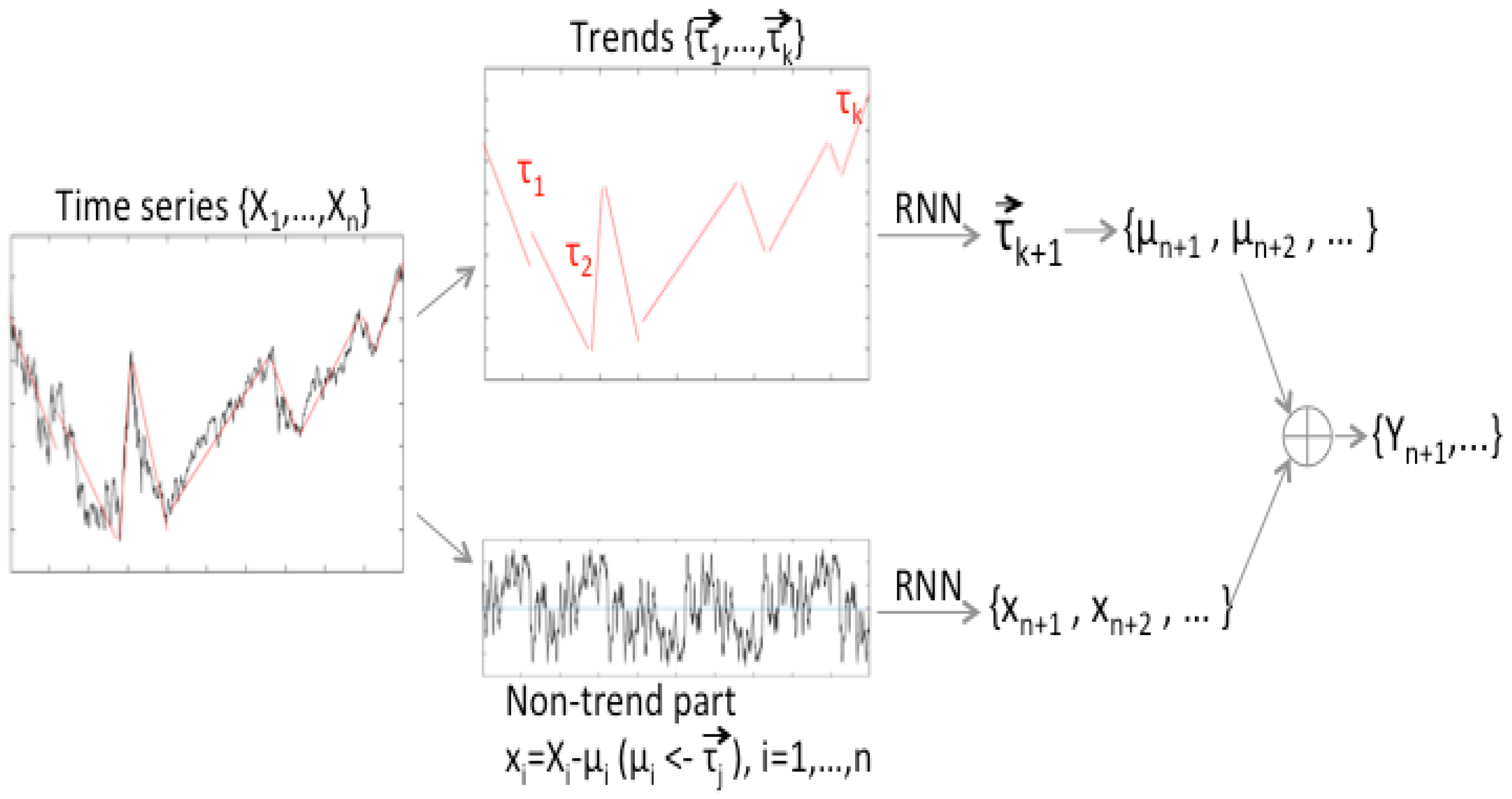
The aim of this paper is to provide a new technique for the prediction of more accurate future trends, using a single-layer RNN structure for a given time-series. For this, first, a trend vector is derived from a given set of data whose components are length (duration), slope, and an adjustment part. Second, a non-trend data part is defined, which is equivalent to the difference between the values of the original data and the trend value defined in the previous step. Additionally, instead of using the original time-series as the input of the learning and training mechanism, the previously defined 1 by 3 vector-valued trend and the non-trend parts are used as the input for the learning process. Note that, for the most part of the paper, the simple RNN is the default training method, which was chosen to emphasize the strength of trend methods; that is, even with one of the simplest learning schemes, the forecasting results are better than some variance of RNN learning methods, which is a motivation and strength of this work. This is also demonstrated by the examples and numerical experiments, in which the use of both trend and non-trend data parts results in better prediction performance. A brief explanation of this process is shown in Figure 1.

2. Obtaining the Trend from Training Data

In this section, we explain a new approach to finding linear trends in a given time-series.

2.1. Definition of Trend

From the given data of a total learning data set $TLS=\{X_1,X_2,\dots ,X_n\}$, where n is the length of the data, a set of linear trends $\{{\overrightarrow{\tau }}_1,{\overrightarrow{\tau }}_2,\dots ,{\overrightarrow{\tau }}_k\},(k<n)$ is taken, where each trend ${\overrightarrow{\tau }}_j$ is a vector with three components, given as

$${\overrightarrow{\tau }}_j=〈{\ell }_j,s_j,{\epsilon }_j〉,$$

(1)

where

$$\sum _{j=1}^k({\ell }_j-1)=n-1.$$

(2)

and ${\ell }_j$ represents the duration of the j-th trend ${\overrightarrow{\tau }}_j$ in time domain; that is,

$${\ell }_j=t_{{\tau }_{j+1}}-t_{{\tau }_j}+1,$$

(3)

where $t_{{\tau }_k}$ represents the time value at which the k-th trend starts and $s_j$ represents the (linear) slope of ${\overrightarrow{\tau }}_j$,

$$s_j=arctan(\frac{X_{{\tau }_{j+1}}-X_{{\tau }_j}}{{\ell }_j})$$

(4)

where $X_{{\tau }_k}$ is the first data value of the k-th trend. The set of data $TLS$ is represented as k subsets $L{S}_j$s as

$${\cup }_{j=1}^{k}L{S}_j=TLS,$$

(5)

where the intersection of $L{S}_j$ and $L{S}_{j+1}$ (i.e., $L{S}_j\cap L{S}_{j+1}$) is a single element on the boundary of the two trend lines. The elements of $L{S}_j$ are data values with respect to the time domain $\{1+{\sum }_{t=1}^{j-1}({\ell }_t-1),\dots ,1+{\sum }_{t=1}^j({\ell }_t-1)\}$.

2.2. Defining the Trend Value ${\mu }_i$

In detail, the durations ${\ell }_1,{\ell }_2,\dots ,{\ell }_k$ and the slopes $s_1,s_2,\dots ,s_k$ of all trends are calculated by the following technique: First, in the total learning set $TLS$ (see Equation (5)), pick a maximum-valued element and a minimum-valued element and label them as $X_{{max}_1}$ and $X_{{min}_1}$, respectively. If there are more than one occurrences of maximum or minimum, just choose one. In our algorithm, we chose the first one (i.e., at the smallest time index). Assume that $ma{x}_1<mi{n}_1$ (note that the other case works in the same manner). Then, link the first data $X_1$ to $X_{ma{x}_1}$, $X_{ma{x}_1}$ to $X_{mi{n}_1}$, and $X_{mi{n}_1}$ to the last data $X_n$ in the graph of the time-series $TLS$. From this first process, we have three subsets $\{L{S}_1^1,L{S}_2^1,L{S}_3^1\}$, where $L{S}_1^1=\{X_1,\dots ,X_{ma{x}_1}\},L{S}_2^1=\{X_{ma{x}_1},\dots ,X_{mi{n}_1}\}$ and $L{S}_3^1=\{X_{mi{n}_1},\dots ,X_n\}$ as shown in Figure 2. The linear lines produced by linking the end points of $L{S}_j^1$$(j=1,2,3)$ are the trends, with one dividing process.

In Figure 2, Korea Composite Stock Price Index (Kospi) data (http://kr.investing.com) with a data length of 3800 was used as an example for showing how the trends are calculated. If the first or the last data is one of the maximum or minimum values, there are only one or two trends. The next step is to divide each $L{S}_j^1(j=1,2,3)$ into one, two, or three subsets, through a similar process.

From now, we will change the data value into ${\{X_i-{\mu }_i\}}_{i=1,\dots ,n}$ where ${\mu }_i$ is the value of the linear trend at $t=i$. For example, in $L{S}_1^1=\{X_1,\dots ,X_{ma{x}_1}\}$, ${\mu }_i$ is a trend value at time i for $i=1,\dots ,ma{x}_1$ and is determined from a linear function which connects $X_1$ and $X_{ma{x}_1}$; that is, ${\mu }_i$ is calculated as

$${\mu }_i=\left\{\begin{array}{cc}{X}_1\hfill & \mathrm{if}i=1\hfill \\ \frac{X_{ma{x}_1}-X_1}{ma{x}_1-1}(i-1)+X_1\hfill & \mathrm{if}1<i<ma{x}_1\hfill \\ X_{ma{x}_1}\hfill & \mathrm{if}i=ma{x}_1.\hfill \end{array}\right.$$

(6)

Note that ${\mu }_i$ is changed when dividing the subsets of $LS$.

Then $L{S}_1^1$ produces subsets $L{S}_1^2,L{S}_2^2$ and $L{S}_3^2$ with respect to the new indices $ma{x}_2,mi{n}_2$, where $ma{x}_2,mi{n}_2$ represents the indices of the maximum and minimum data value of ${\{X_i-{\mu }_i\}}_{i=1,\dots ,ma{x}_1}$, and so on. To stop reproducing subsets and complete the making the trend data set, a reasonable threshold is needed. This procedure keeps repeating until the difference between the maximum and the minimum value of a modified data subset is smaller than the threshold. In our experiments the threshold is chosen depending on the data set. If the threshold is not small enough, the trend value might not be able to represent the flow of the time-series data well and also the number of trends is too small to execute the learning with the trend set. Thus, to obtain a suitable number of trends, we need to have a smaller threshold. 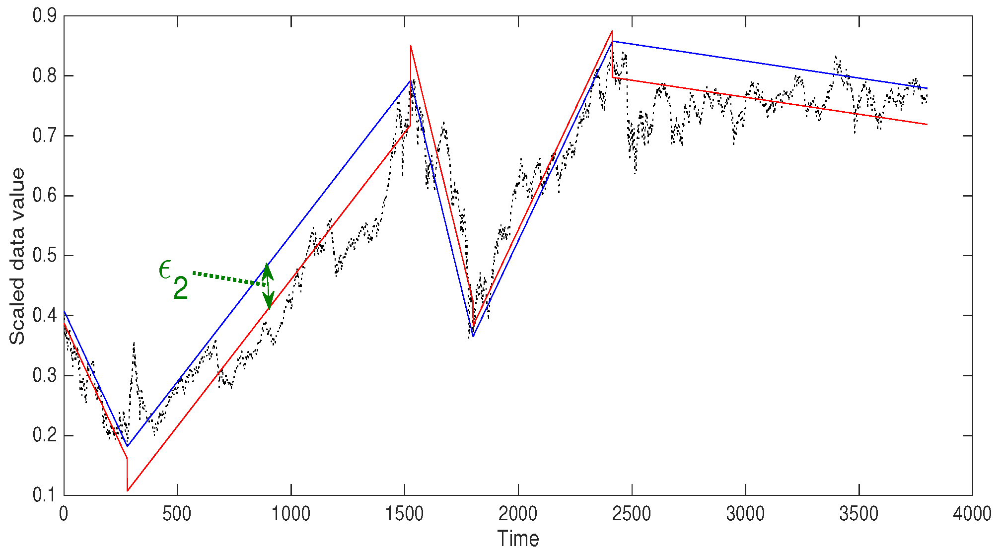Figure 3 shows an example of using a threshold. A threshold of 0.5 was used for a Kospi data subset with length 3800. Finding linear trends, the blue lines, is done after scaling data by dividing by the maximum value of the total data set so the threshold is less than 1. It is shown that with the threshold 0.5, the number of the trends of this data is 5 which is too small for the number of learning data set and not enough to catch the non-ignorable bumps in the time-series. For finding a reasonable threshold, more detailed explanation is described in the next section.

After obtaining the final set of linear trends, the j-th trend can be expressed as its duration ${\ell }_j$ and the slope $s_j$ of the line for $j=1,\dots ,k$ where k is the number of trends.

2.3. Defining ${\ell }_j$ and $s_j$

Note that the trend between $X_p$ and $X_q$ lies on the time interval $[p,q]$. (i.e., $q-p+1$ is the number of trend data) and the corresponding duration ${\ell }_j$ is defined as

$${\ell }_j=q-p+1.$$

(7)

Furthermore, the slope $s_i$ of the trend can be defined as the angle from the slope $(X_q-X_p)/(q-p)$, where p and q are the indices of the endpoints of the trend. We use the radian value of the angle from the inverse tangent of the slope; that is,

$$s_j=arctan(\frac{X_q-X_p}{q-p}),$$

(8)

which is a real number between $-\frac{\pi }{2}$ and $\frac{\pi }{2}$. Examples of ${\ell }_j$ and $s_j$ are shown in Figure 2.

2.4. Defining ${\epsilon }_j$

The next step is to adjust and to update each trend set from a vector of two elements, ${\ell }_j$ and $s_j$, to a vector of three elements with the following rule: In the j-th trend (for example), for a time-series data value in the trend set $X_i\in L{S}_j$, calculate the expectation value of all $X_i-{\mu }_i$ and denote it by ${\epsilon }_j$, where $X_i$ is a data value in j-th trend ${\tau }_j$. That makes

$$\sum _{X_i\in L{S}_j}(X_i-{\mu }_i-{\epsilon }_j)=0.$$

(9)

Define the j-th trend as

$${\overrightarrow{\tau }}_j=〈{\ell }_j,s_j,{\epsilon }_j〉,$$

(10)

where $j=1,\dots ,k$. Now, this is equivalent to a linear function with slope $s_j$ with duration ${\ell }_j$ from the first point of $L{S}_j$, and with ${\epsilon }_j$ subtracted; that is, define an adjusted trend value ${\mu }_i^{\prime }={\mu }_i+{\epsilon }_j$, represented by ${\overrightarrow{\tau }}_j$ where ${\{{\overrightarrow{\tau }}_i\}}_{i=1,\dots ,k}$ satisfies

$$\mathbb{E}(X_i-{\mu }_i^{\prime })=0$$

(11)

for all $X_i\in L{S}_j$. These are shown as red line segments in Figure 3.

Now, it remains to train a RNN on the two different time-series, in order to predict the next unknown data. One is the adjusted trend set $\{{\overrightarrow{\tau }}_1,{\overrightarrow{\tau }}_2,\dots ,{\overrightarrow{\tau }}_k\}$ and the other is the non-trend data ${\{x_i=X_i-{\mu }_i^{\prime }\}}_{i=1,\dots ,.n}$. By learning the trend set, we can predict the length and duration of the next trend. The expected value of the non-trend part is trained. The algorithm, so far, can be expressed as the following.

3. Finding a Threshold

In this section, we describe a method to obtain a reasonable threshold for Algorithm 1. As mentioned in the previous section, subsets of given data are divided until the biggest difference between the divided trend and the data is less than the threshold.

Algorithm 1: Obtaining the Trend Set

Set an index set as $\mathit{Index}=\{1,n\}$, where n is the number of the training data. Find $ma{x}_1,mi{n}_1$ such that $max(X_1,\dots ,X_n)=X_{ma{x}_1},min(X_1,\dots ,X_n)=X_{mi{n}_1}$ and add these to the Index set (i.e., $\mathit{Index}=\{1,ma{x}_1,mi{n}_1,n\}$). Get rid of duplicate indices and sort the set. For $L{S}_i^1=\{X_{\mathit{Index}(i)},\dots ,X_{\mathit{Index}(i+1)}\}$ for $i=1,\dots ,(\#\mathrm{of}\mathit{Index}-1)$, link $X_{\mathit{Index}(i)}$ and $X_{\mathit{Index}(i+1)}$ and let ${\mu }^1(j)$ be the value of the linked linear line. For each $\{X_j-{\mu }_j\}$, $j=1,\dots ,n$, find $max$ and $min$ indices and repeat Steps 2 and 3. Repeat Step 4 until $|X_{max}-X_{min}|\le \mathit{threshold}$ for a pre-chosen threshold.

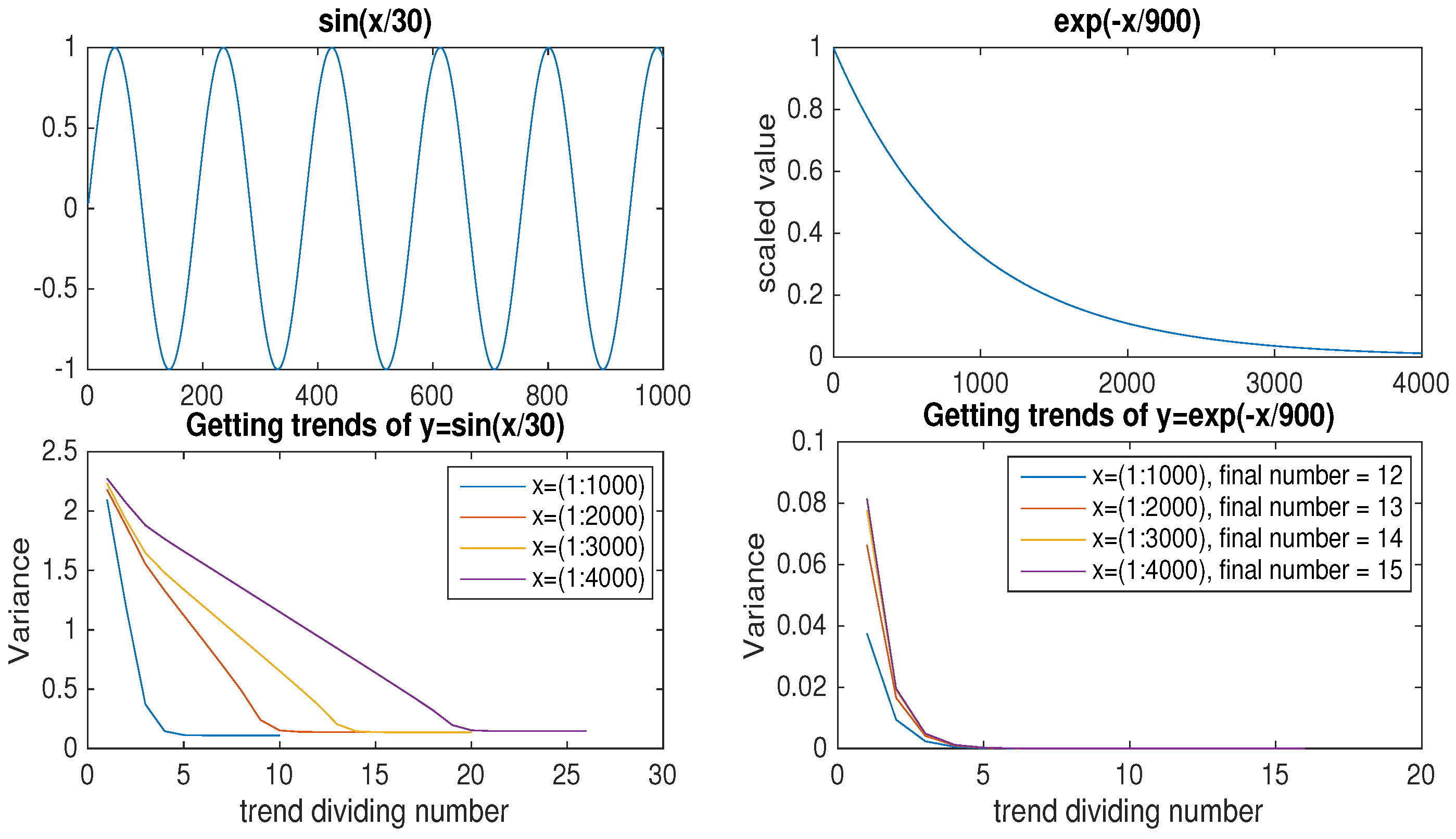
Before obtaining trends of real data, such as a financial series or temperature data, let us consider some examples of data. As periodicity is an important factor among the many characteristics of data, we consider periodic and non-periodic example data to figure out suitable thresholds for each type of data. For the periodic example, consider $X_i=sin(\frac{i}{30})$ for $i=1,\dots ,n$ and, for the non-periodic one, consider $X_i=exp(-\frac{i}{900})$ for $i=1,\dots ,n$. Note that the data is used after scaling by the maximum absolute value of the data, such that it is bounded in $[-1,1]$. After applying the dividing domain methods mentioned in the previous section with a very small threshold (say, 0.00001), we obtain the $L{S}_i$s; the subsets of the total learning set $TLS={\{X_i\}}_{i=1,\dots ,n}$.

By varying the different number of data n between 1000, 2000, 3000, and 4000, we can make observations about the variance of the difference between data and the trend per division of the trends. If ${\mu }_i^{\prime }$$(i=1,\dots ,n)$ represents an adjusted trend value after a certain amount of trend division, we define the variance as

$$variance=\frac{1}{\#TLS}\sum _{X_i\in TLS}{(X_i-{\mu }_i^{\prime })}^2,$$

(12)

where $X_i$ is an element at time i in the total learning set and ${\mu }_i$ is the corresponding trend value at time i.

Figure 4 plots the variance of two example data per trend division number as the number of data was increased by 1000. As the trigonometric function had a proportional number of extremes to the total length data, the trend division number was also proportional to the total length. We can observe that the first variance (i.e., the variance after the first trend division) was similar after increasing the size of data and, also, that the final variance barely changed, even when the length of the data was increased. However, for non-periodic data (the exponential function, in our example), the first variance increased as the size of the data increased. It took a lot of divisions to approach the goal after getting near the final variance (with a small threshold 0.00001) for the non-periodic data, while the periodic data stopped trend division shortly after getting near the final variance.

From this observation, we can get a hint if the given data is periodic or not by calculating variance per trend division with different sized sets of the data (i.e., we can do a pre-processing to get the periodicity of a data). After pre-processing, if a data is periodic or periodic-like, we can choose a small portion of the data and choose the threshold depending on the amount of data difference one wants to ignore when setting trends.

The above method suggests a way to find a suitable threshold; however, changing threshold results in different trend lengths which may affect interpretation of various aspects of the data. The length of the trend does not affect the accuracy of learning, so using different thresholds with various goals of forecasting is possible.

4. Learning the Trend

In this section, we want to train a set $\{{\overrightarrow{\tau }}_1,{\overrightarrow{\tau }}_2,\dots ,{\overrightarrow{\tau }}_k\}$, where ${\overrightarrow{\tau }}_j$ is a $1\times 3$ vector, for $j=1,\dots ,k$, where k is the number of trends (see Equation (10)). As we have a $1\times 3$ vector ${\overrightarrow{\tau }}_t$ as the t-th input of the simple RNN process, the dimension of ${\overrightarrow{h^{\tau }}}_t$ and ${\overrightarrow{y^{\tau }}}_t$, which are the t-th hidden state and the output value of trend, respectively, can be set as vectors of size $1\times 3$, as shown in the following equations:

$$\begin{array}{ccc}\hfill {\overrightarrow{y^{\tau }}}_t& =& W_y^{\tau }{\overrightarrow{h^{\tau }}}_t+\overrightarrow{b_y^{\tau }},\hfill \end{array}$$

(13)

$$\begin{array}{ccc}\hfill {\overrightarrow{h^{\tau }}}_t& =& tanh(W_h^{\tau }{\overrightarrow{h^{\tau }}}_{t-1}+W_{\tau }^{\tau }{\overrightarrow{\tau }}_t+\overrightarrow{b_h^{\tau }}),\hfill \end{array}$$

(14)

where $W_y^{\tau },W_h^{\tau }$ and $W_{\tau }^{\tau }$ are in ${\mathbb{R}}^{3\times 3}$ and $\overrightarrow{b_y^{\tau }}$ and $\overrightarrow{b_h^{\tau }}$ are in ${\mathbb{R}}^{1\times 3}$. Note that we need to calculate the matrix–vector multiplications in the opposite order; for example, we calculate $W_y^{\tau }{\overrightarrow{h^{\tau }}}_t$ as ${\overrightarrow{h^{\tau }}}_t·W_y^{\tau }$ to match the dimension of the result vector. The goal of this training is to get an approximated set of weights and biases which minimise the cost function

$$\begin{array}{ccc}\hfill cost& =& \frac{1}{trai{n}^{\tau }-se{q}^{\tau }}\sum _{i=se{q}^{\tau }}^{trai{n}^{\tau }-1}\left|\right|{\overrightarrow{y^{\tau }}}_i-{\overrightarrow{\tau }}_{i+1}{\left|\right|}_2^2\hfill \end{array}$$

(15)

$$\begin{array}{cc}=& \frac{1}{trai{n}^{\tau }-se{q}^{\tau }}\sum _{i=se{q}^{\tau }}^{trai{n}^{\tau }-1}\left|\right|W_y^{\tau }tanh(W_h^{\tau }{\overrightarrow{h^{\tau }}}_{t-1}+W_{\tau }^{\tau }{\overrightarrow{\tau }}_t+\overrightarrow{b_h^{\tau }})+\overrightarrow{b_y^{\tau }}-{\overrightarrow{\tau }}_{i+1}{\left|\right|}_2^2,\hfill \end{array}$$

(16)

where ${\left|\right|.\left|\right|}_2$ is the ${\ell }_2$-norm, $trai{n}^{\tau }$ is the number of trends for training (which is k, in this case), and $se{q}^{\tau }$ is the sequence length for trend training. The cost is defined as the average value of all differences squared, as shown in (15). We use the Adam optimisation method to minimise this cost and get the optimum weight and bias sets [26].

Once a trend set is well-trained, a prediction of the next trend ${\overrightarrow{\tau }}_{k+1}=〈{\ell }_{k+1},s_{k+1},{\epsilon }_{k+1}〉$ can be generated, which is close to the real future data.

5. Learning the Non-Trend Part

In the previous section, we obtained a prediction of trend which adequately predicts the flow of the data. Now, the remaining oscillating, noise-like part is the non-trend part of the data. There are two different methods of forecasting suggested in this paper. One is considering the non-trend data as a time-series with same length as the original data and using the same scheme, simple RNN, with trend training. The other is calculating the expected bounds of non-trend part from the minimum and the maximum value of non-trend part in each trend.

5.1. Simple RNN Method

First, the non-trend part can be also trained using the simple RNN process and produce a set of prediction values $\{y_t\}$ by the following equations,

$$\begin{array}{ccc}\hfill y_t& =& w_y{h}_t+b_y,\hfill \end{array}$$

(17)

$$\begin{array}{ccc}\hfill h_t& =& tanh(w_h{h}_{t-1}+w_x{x}_t+b_h),\hfill \end{array}$$

(18)

and this result can be added to the obtained trend. It is identical to the simple RNN process, but the input data is given as the original scaled data with the trend prediction from the previous process subtracted; that is,

$$x_t=X_t-{\mu }_t^{\prime },$$

(19)

where ${\mu }_t^{\prime }$$(t=1,\dots ,n)$ represents the data value of the corresponding trend ${\overrightarrow{\tau }}_i$ in the trend set ${\{{\overrightarrow{\tau }}_i\}}_{i=1,\dots ,k}$. Note that the number of predictions of the non-trend part is limited to the length of the predicted trend, since we are only interested in the movement of the data in that trend. For instance, in the previous section, after the trend training, the $(k+1)$-th trend $〈{\ell }_{k+1},s_{k+1},{\epsilon }_{k+1}〉$ is obtained. So, only ${\ell }_{k+1}$ number of predictions $\{y_{n+1},y_{n+2},\dots ,y_{n+{\ell }_{k+1}}\}$ are obtained from the non-trend training.

Combining this non-trend part and the trend training result from the previous subsection, the final prediction is obtained as

$$Y_t={\mu }_t^{\prime }+y_t,$$

(20)

where ${\mu }_t^{\prime }$ is the data value of ${\overrightarrow{\tau }}_{k+1}$ and $y_t$ is the non-trend prediction result for $t=1,\dots ,{\ell }_{k+1}$. The algorithm, so far, can be expressed by the following algorithm (Algorithm 2). Note that, in Step 1, in the form of the trend, the third element ${\epsilon }_i$ is a value obtained to make the average of the data with the trend subtracted zero in each trend. Also, note that, in Step 3, it uses the optimisation scheme with three variables.

Algorithm 2: Forecasting by Learning Trend and Non-trend Parts

Take a trend set of the data with a form of 〈length,slope,error〉 (i.e., ${\overrightarrow{\tau }}_i=〈{\ell }_i,s_i,{\epsilon }_i〉$, $i=1,\dots ,k$ for some k). Obtain the hidden layer values and output values after the simple RNN process (as in Equation (13)). Perform the Adam optimisation scheme with suitable iteration number to get a minimum of the trend cost (Equation (15)). From Step 3, get a prediction of upcoming trend after the training data set ${\overrightarrow{\tau }}_{k+1}=〈{\ell }_{k+1},s_{k+1},{\epsilon }_{k+1}〉$. Take a non-trend set of the data by subtracting the original data by the trend value from Step 1. Get hidden layer values and output values after simple RNN process with one variable input. Perform the Adam optimisation scheme with suitable iteration number to get a minimum of the non-trend cost. From Step 7, get predictions of the non-trend values. Note that the number of predictions is equivalent to the length ${\ell }_{k+1}$ of the predicted trend ${\overrightarrow{\tau }}_{k+1}$. Combine the results from Steps 4 and 8.

5.2. Bound Training Method

Another method for dealing with the non-trend part is by training the bounds of the non-trend value in each trend. First, we calculate the maximum and minimum values of $X_j-{\mu }_j^{\prime }$ in each trend for $j=1,\dots ,n$ where $X_j$ is the data value and ${\mu }_j^{\prime }$ represents the trend value for a trend length n. Then, there are k pairs of maximum and minimum values (i.e., ${\{(ma{x}_i,mi{n}_i)\}}_{i=1,\dots ,k}$, where k is the number of trends of the data). This can be considered as a time-series as well, so the RNN can be used again with this series of vectors with two elements. The hidden state vector ${\overrightarrow{y^{n\tau }}}_t$ and the output value vector ${\overrightarrow{h^{n\tau }}}_t$ for non-trend part are both $1\times 2$ vectors and satisfy the following equations

$$\begin{array}{ccc}\hfill {\overrightarrow{y^{n\tau }}}_t& =& W_y^{n\tau }{\overrightarrow{h^{n\tau }}}_t+\overrightarrow{b_y^{n\tau }},\hfill \end{array}$$

(21)

$$\begin{array}{ccc}\hfill {\overrightarrow{h^{n\tau }}}_t& =& tanh(W_h^{n\tau }{\overrightarrow{h^{n\tau }}}_{t-1}+W_{n\tau }^{n\tau }{\overrightarrow{\tau }}_t+\overrightarrow{b_h^{n\tau }}),\hfill \end{array}$$

(22)

where the weight matrix for non-trend part $W_y^{n\tau },$$W_h^{n\tau }$, and $W_{n\tau }^{n\tau }$ are in ${\mathbb{R}}^{2\times 2}$ and the bias vector for the non-trend part $\overrightarrow{b_y^{n\tau }}$ and $\overrightarrow{b_h^{n\tau }}$ are in ${\mathbb{R}}^{1\times 2}$ for $t=1,\dots ,k$. As a result of optimisation of the above equations, predictions for the maximum and the minimum for the non-trend values are produced.

6. Numerical Experiments

In this section, some numerical results of the proposed schemes—RNNs for trend, RNNs for non-trend, and the combination of these two—are shown through two examples of practical data.

6.1. Stock Market Index Data

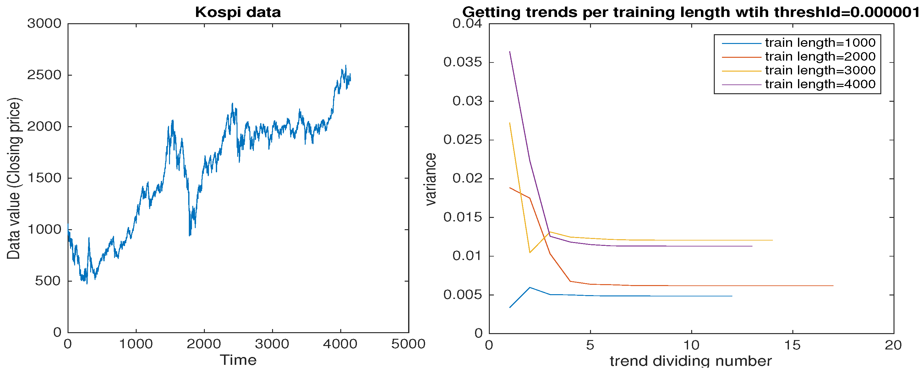
The first example is the Korea Composite Stock Price Index (Kospi) closing price data, which was used in Section 2. In this experiment, the number of the data was over 4200. As shown in Figure 5, pre-processing of this data gave the flow of variance of the non-trend part by trend division per length of data. The variance value converged fast and remained near convergence for over 70 percent of the trend division time; this behavior of convergent time was the same for all lengths of regularly chopped data. This is similar to the result for the exponential function data in Section 3, so the Kospi data can be considered to be a non-periodic data type. Thus, the choice of a threshold for the trend division should be small (i.e., 0.00001), in order to catch the number of trends.

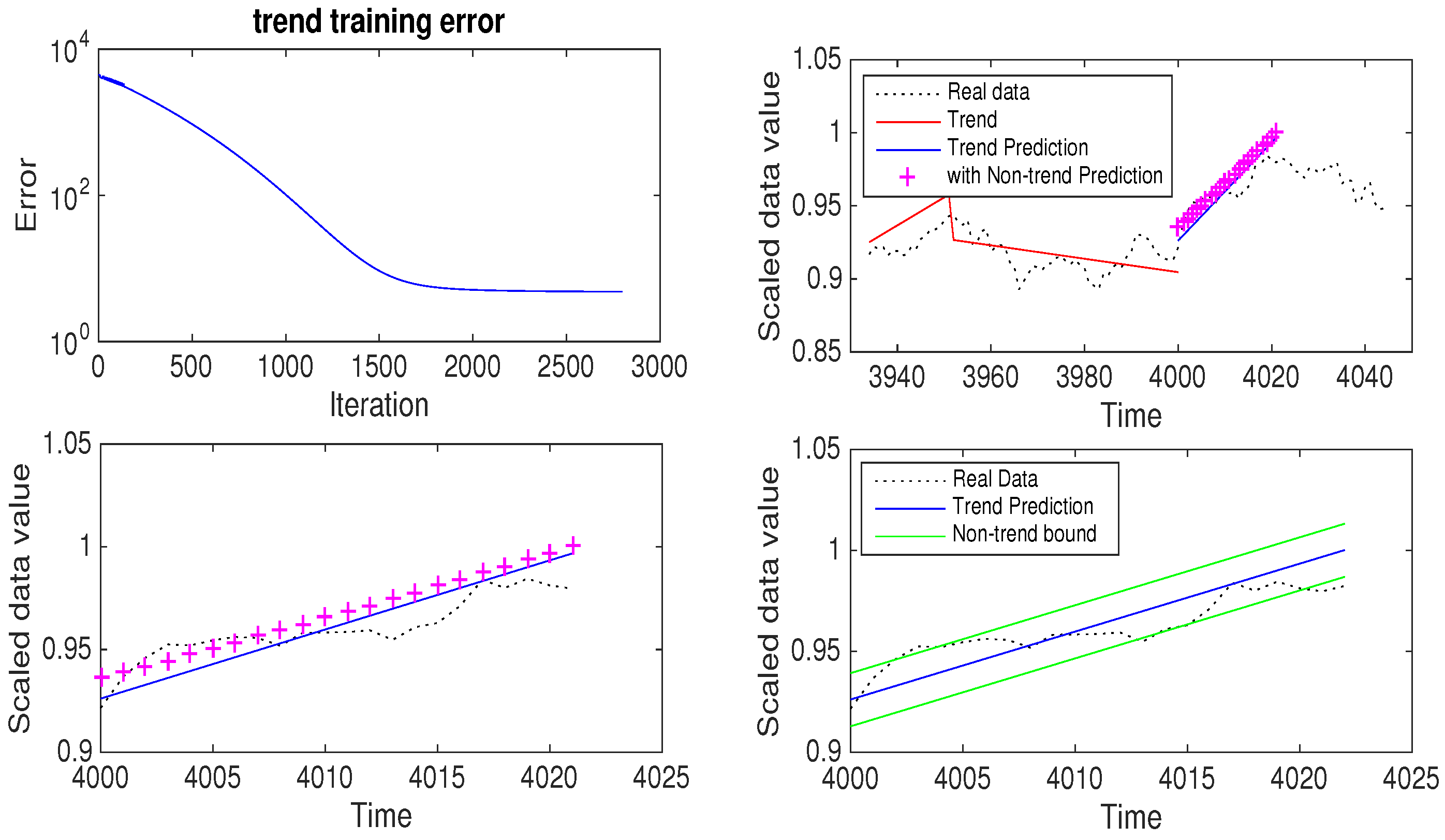
The number of trends with threshold 0.00001 was 274 and the threshold which gave the closest number of trends was 0.05. So, for this experiment, the training data length was 4000 and the threshold was 0.05. In Figure 6, the data and its trend are given in the first graph and the (decreasing) trend of learning error in the second graph. This shows that the trend learning worked well. With this threshold, the number of trends was 178 and (as we used 1/10 of the number of trends) 17 was the sequence length. A total of 2800 iterations were used for the learning of this trend set.

After learning the trend, it predicted the next trend which turned out to be 22, 0.003364, and 0.004562 as the duration, slope, and adjustment, respectively. See the third and fourth graphs in Figure 6 for closer look at the prediction part. We can see that this scheme worked well in finding the next trend. For the non-trend part, the training length was the same as the total data number used to obtain the trends. The sequence length of the non-trend part was decided as the floor function of the length of the training data divided by the length of the trend obtained from the previous step. So, for this example, the sequence length of the non-trend training was $⌊4000/178⌋=22$. The number of iterations for the non-trend part learning was 3000.

6.2. Temperature Data

The next data set was temperature data. It is the monthly average temperature measured in Seoul, South Korea and the data length was over 24,000. Similar to the the previous data, Figure 7 shows the variance information of the non-trend part as changing trends per length of regularly chopped data. From this graph, the convergent time of variance for each data length varied and was proportional to the length of the training data. Given this pre-processing result, the temperature data was determined to be periodic/periodic-like and, so, the threshold for obtaining trends was chosen as needed. In this experiment, a threshold of 0.5 suited our purposes. Thus, a training data length of 23,000 and a threshold of 0.5 were used. Then, 988 trends were obtained with this threshold and, so, the sequence length for trend learning was set to 98, calculated similarly to the previous case. In Figure 8, the data and its trends are shown in the first graph and the decreasing trend learning error in the second graph. We can see that the trend learning worked well. With a sequence length of 98 and 23,000 iterations, the trend learning gave that the duration, slope, and adjustment of the next trend were 23, −0.012443, and −0.000828 respectively. In Figure 8, this result is shown visually, where the fourth graph shows a closer look of the prediction part. For the non-trend part, 5000 iterations were used.

7. Comparison with Other Methods in the Numerical Experiments

In this section, we will compare the detection results of our scheme with other existing forecasting methods.

7.1. Comparison with Other Trend Methods

There are many statistical methods and techniques for the forecasting of time-series. Among these methods, averaging-based methods are typically used to compare forecasting results. The first method used was the single exponential smoothing method [27]. The smoothed value is given by

$$S_{t+1}=\alpha {\mathrm{y}}_{origin}+(1-\alpha )S_t,0<\alpha \le 1,t\ge 3,$$

(23)

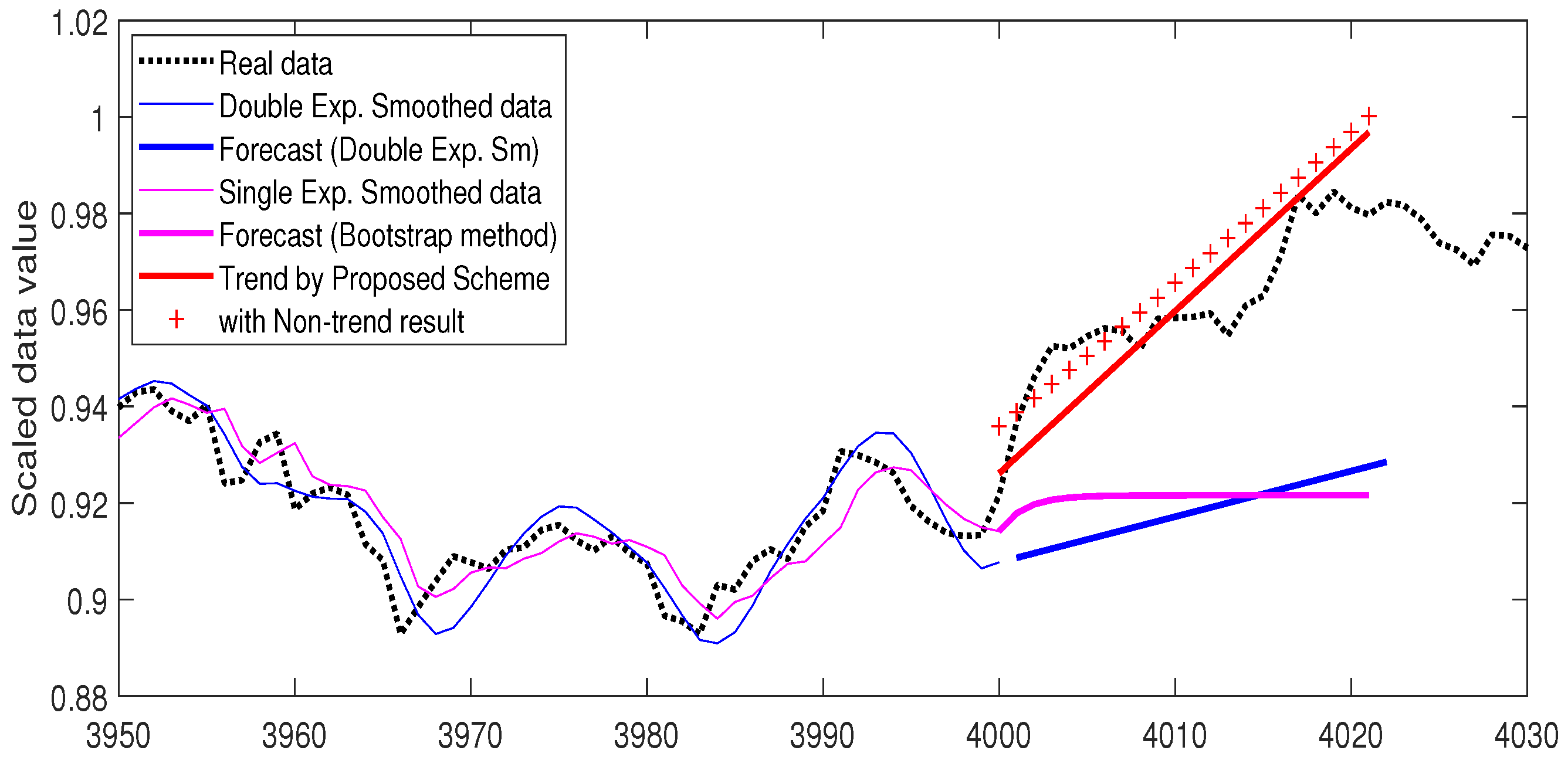
where ${\mathrm{y}}_{origin}$ remains constant for all future forecast calculations, which is known as bootstrapping [28]. The parameter $\alpha$ is determined by minimizing the mean squared error (MSE). We used this bootstrapping forecasting method for comparison. See Figure 9 and Figure 10 for the comparison forecasting results of the Kospi and temperature data, respectively. The thin pink line is the data smoothed with the single exponential method and the thick pink line represents the forecast value using the bootstrap method.

The next averaging method we used was double exponential smoothing [29]. It uses two constants and is known to handle trends more efficiently. The equation is obtained as follows

$$\begin{array}{ccc}\hfill S_t& =& \alpha {\mathrm{y}}_t+(1-\alpha )(S_{t-1}+b_{t-1})\hfill \end{array}$$

(24)

$$\begin{array}{ccc}\hfill b_t& =& \gamma (S_t-S_{t-1})+(1-\gamma )b_{t-1},\hfill \end{array}$$

(25)

where $\alpha$ and $\gamma$ are determined using non-linear optimisation techniques. The m-period-ahead forecast is obtained by

$$F_{t+m}=S_t+m{b}_t.$$

(26)

In Figure 9 and Figure 10, the thin blue line represents the double exponential smoothed data and the thick blue line shows the linear forecasting result $F_{t+m}$.

In both data examples, the red line shows the predicted trend with our proposed scheme and the series of points marked with + indicates the trend prediction added by the non-trend part predictions. It can be observed, in both figures, that our proposed scheme detected the real data more accurately. See

Table 1. Comparison of mean squared errors (MSEs) with exponential smoothing methods.

	Kospi	Temperature
Single exponential smoothing method	0.0018	0.1057
Double exponential smoothing method	0.0020	0.1958
Proposed scheme	1.2329 × 10${}^{-4}$	0.0372

for the calculated mean squared errors of each method, for both Kospi and temperature data sets, in Figure 9 and Figure 10.

7.2. Comparison with Other Learning Methods

In this sub-section, we compare our proposed method with other learning schemes, such as simple RNN and simple LSTM (both with a single layer). We used a simple version of these schemes on the Kospi data, and the prediction results are shown in Figure 11. With the same training number (4000), the result of LSTM popped up and down, back to around 1.35 at the time 4007, whereas the result of RNN stayed around the real data value. Thus, our result (the red line in the Figure 11), which was closest to the real data, gave the best prediction among these methods. See

Table 2. Comparison of MSEs with other learning methods.

	Kospi
Simple RNN	0.0105
Simple LSTM	0.4024
Proposed scheme	1.2329 × 10${}^{-4}$

for a comparison of the mean squared errors of each learning method. A comparison using the temperature data gave a similar result, as this is from the simple RNN variances which have some issues (such as vanishing gradient).

8. Conclusions and Future Works

In this paper, we introduced a new algorithm to predict future data from given time-series data by finding trends in the data set which fit into the given data and, then, applying existing simple recurrent neural network learning to them. Here, we propose a technique to collect and find the trend set with three pieces of information—slope, duration, and adjustment. Once the trends set has been collected, it is trained by a simple RNN, such that future trends can be predicted. Additionally, to increase the accuracy of the prediction, we considered the non-trend part in the time-series. A simple RNN was also trained on the non-trend parts and the results were added to the prediction of the trends.

Through several numerical simulations, it was shown that the collected trends can fit the given time-series data and are also well-trained, such that the prediction of future trends is accurate, compared to the real data. Furthermore, the accuracy could be increased by adjusting the trend prediction by training on the non-trend part. Note that all training simulations were executed by a simple, single-layer RNN, due to hardware limitations. Hence, in order to fully explore the efficiency of the proposed algorithm, we will combine the proposed algorithm with LSTM or GRU, instead of using only a simple RNN, since those variants of RNN are well-known to be better predictors in RNN structures [30,31].

References

- Atsalakis, G.S.; Valavanis, K.P. Forecasting stock market short-term trends using a neuro-fuzzy based methodology. Expert Syst. Appl. 2009, 36, 10696–10707. [Google Scholar] [CrossRef]
- Box, G.; Jenkins, G.; Reinsel, G. Time Series Analysis: Forecasting and Control; Prentice Hall: Upper Saddle River, NJ, USA, 1994. [Google Scholar]
- Dangelmayr, G.; Gadaleta, S.; Hundley, D.; Kirby, M. Time series prediction by estimating markov probabilities through topology preserving maps. In Applications and Science of Neural Networks, Fuzzy Systems, and Evolutionary Computation II; International Society for Optics and Photonics: Bellingham, WA, USA, 1999; Volume 3812, pp. 86–93. [Google Scholar]
- Graves, A.; Schmidhuber, J. Framewise phoneme classification with bidirectional LSTM and other neural network architectures. Neural Netw. 2005, 18, 602–610. [Google Scholar] [CrossRef] [PubMed]
- Hosseini, S.; Khaled, A.A.; Vadlamani, S. Hybrid imperialist competitive algorithm, variable neighborhood search, and simulated annealing for dynamic facility layout problem. Neural Comput. Appl. 2014, 25, 1871–1885. [Google Scholar] [CrossRef]
- Jin, Z.; Zhou, G.; Gao, D.; Zhang, Y. EEG classification using sparse Bayesian extreme learning machine for brain—Computer interface. Neural Comput. Appl. 2018, 1–9. [Google Scholar] [CrossRef]
- Keogh, E.J. A decade of progress in indexing and mining large time series databases. In Proceedings of the 32nd International Conference on Very Large Data Bases, Seoul, Korea, 12–15 September 2006; pp. 1268–1268. [Google Scholar]
- Khaled, A.A.; Hosseini, S. Fuzzy adaptive imperialist competitive algorithm for global optimization. Neural Comput. Appl. 2015, 26, 813–825. [Google Scholar] [CrossRef]
- Zhang, X.; Yao, L.; Wang, X.; Monaghan, J.; Mcalpine, D.; Zhang, Y. A Survey on Deep Learning based Brain Computer Interface: Recent Advances and New Frontiers. arXiv 2019, arXiv:1905.04149. [Google Scholar]
- Zhang, Y.; Wang, Y.; Zhou, G.; Jin, J.; Wang, B.; Wang, X.; Cichocki, A. Multi-kernel extreme learning machine for EEG classification in brain-computer interfaces. Expert Syst. Appl. 2018, 96, 302–310. [Google Scholar] [CrossRef]
- Elman, J.L. Finding structure in time. Cognit. Sci. 1990, 14, 179–211. [Google Scholar] [CrossRef]
- Mueen, A.; Keogh, E. Online discovery and maintenance of time series motifs. In Proceedings of the 16th ACM SIGKDD International Conference on Knowledge Discovery and Data Mining, Washington, DC, USA, 25–28 July 2010; pp. 1089–1098. [Google Scholar]
- Schmidhuber, J. A Local Learning Algorithm for Dynamic Feedforward and Recurrent Networks. Connect. Sci. 1989, 1, 403–412. [Google Scholar] [CrossRef]
- Werbos, P.J. Generalization of backpropagation with application to a recurrent gas market model. Neural Netw. 1988, 1, 339–356. [Google Scholar] [CrossRef] [Green Version]
- Gers, F.A.; Schraudolph, N.N.; Schmidhuber, J. Learning Precise Timing with LSTM Recurrent Networks. J. Mach. Learn. Res. 2002, 3, 115–143. [Google Scholar]
- Hochreiter, S.; Schmidhuber, J. Long Short-Term Memory. Neural Comput. 1997, 9, 1735–1780. [Google Scholar] [CrossRef] [PubMed]
- Bengio, Y.; Simard, P.; Frasconi, P. Learning long-term dependencies with gradient descent is difficult. IEEE Trans. Neural Netw. 1994, 5, 157–166. [Google Scholar] [CrossRef] [PubMed]
- Pascanu, R.; Mikolov, T.; Bengio, Y. On the difficulty of training recurrent neural networks. In Proceedings of the 30th International Conference on Machine Learning (ICML 2013), Atlanta, GA, USA, 16–21 June 2013; pp. 1310–1318. [Google Scholar]
- Rohwer, R. The moving targets training algorithm. In Advances in Neural Information Processing Systems 2; Touretzky, D.S., Ed.; Morgan Kaufmann: San Matteo, CA, USA, 1990; pp. 558–565. [Google Scholar]
- Rumelhart, D.E.; Hinton, G.E.; Williams, R.J. Learning representations by back-propagating errors. Nature 1986, 323, 533–536. [Google Scholar] [CrossRef]
- Schmidhuber, J. A Fixed Size Storage O(n3) Time Complexity Learning Algorithm for Fully Recurrent Continually Running Networks. Neural Comput. 1992, 4, 243–248. [Google Scholar] [CrossRef]
- Xu, X.; Ren, W. A Hybrid Model Based on a Two-Layer Decomposition Approach and an Optimized Neural Network for Chaotic Time Series Prediction. Symmetry 2019, 11, 610. [Google Scholar] [CrossRef]
- Afolabi, D.; Guan, S.; Man, K.L.; Wong, P.W.H.; Zhao, X. Hierarchical Meta-Learning in Time Series Forecasting for Improved Inference-Less Machine Learning. Symmetry 2017, 9, 283. [Google Scholar] [CrossRef]
- Lin, T.; Guo, T.; Aberer, K. Hybrid Neural Networks for Learning the Trend in Time Series. In Proceedings of the Twenty-Sixth International Joint Conference on Artificial Intelligence (IJCAI- 17), Melbourne, Australia, 19–25 August 2017; pp. 2273–2279. [Google Scholar]
- Wang, P.; Wang, H.; Wang, W. Finding semantics in time series. In Proceedings of the 2011 ACM SIGMOD International Conference on Management of Data, Athens, Greece, 12–16 June 2011; pp. 385–396. [Google Scholar]
- Kingma, D.P.; Ba, J.L. Adam: A Method for Stochastic Optimization. In Proceedings of the 3rd International Conference for Learning Representations (ICLR 2015), San Diego, CA, USA, 7–9 May 2015. [Google Scholar]
- Brown, R.G. Smoothing, Forecasting and Prediction; Prentice Hall: Upper Saddle River, NJ, USA, 1962. [Google Scholar]
- Efron, B.; Tibshirani, R. An Introduction to the Bootstrap; Chapman & Hall/CRC: Boca Raton, FL, USA, 1993. [Google Scholar]
- Prajakta, S.K. Time Series Forecasting Using Holt-Winters Exponential Smoothing; Kanwal Rekhi School of Information Technology: Mumbai, India, 2004; pp. 1–3. [Google Scholar]
- Cho, K.; Merrienboer, B.V.; Gulcehre, C.; Bahdanau, D.; Bougares, F.; Schwenk, H.; Bengio, Y. Learning Phrase Representations using RNN Encoder-Decoder for Statistical Machine Translation. arXiv 2014, arXiv:1406.1078. [Google Scholar]
- Cho, K.; Merrienboer, B.V.; Bahdanau, D.; Bengio, Y. On the Properties of Neural Machine Translation: Encoder-Decoder Approaches. arXiv 2014, arXiv:1409.1259. [Google Scholar]
© 2019 by the authors. Licensee MDPI, Basel, Switzerland. This article is an open access article distributed under the terms and conditions of the Creative Commons Attribution (CC BY) license (http://creativecommons.org/licenses/by/4.0/).