Abstract
This paper presents an innovative computer graphic method for viewshed generation from big point clouds. The proposed approach consists in simplification of typical methods for viewshed formation that are based on sorting and binary trees. The proposed method is based on the k-d tree concept optimized with radial segmentation and a dedicated mathematical algorithm for subtree rejection. The final visualization of the viewshed is designed with a graphic method using triangulated irregular network (TIN) surfaces from the accepted subtrees.
1. Introduction
1.1. Background
At present, emotions arising from the surrounding landscape greatly affect human wellbeing. More and more people would like to prevent the destruction of natural landscape and its monuments in an ill-conceived pursuit for financial profit. We want to experience beauty in the historic districts of our cities, outside our windows, and far away from the urban areas: in the mountains, forests, meadows, and parks.
Information about natural resources is increasingly collected by virtue of a variety of terrain scanning methods. As a result, more and more data are created, which include point clouds. Due to the increasing technological possibilities, the obtained point clouds have an enhanced density, and that makes them more detailed [1,2]. Therefore, the development of acquisition methods must be accompanied by the development of software for their rapid processing. In many cases, the amount of data is so large that only a well-prepared environment enables their practical use.
The main use of point clouds, which the authors focus on, is to generate a viewshed. Viewsheds can be, among others, applied to study to what extent a newly designed building affects the surrounding landscape [3]. There are many cases of investments for which such analyses were not carried out, and it resulted in their negative impact on the observation of surrounding monuments from various viewpoints.
Another application is to perform an analysis of the area visible to the surveillance cameras [4]. Such an analysis indicates the areas visible to a camera from a given place, which leads to the optimal distribution of the objects in a given space. The area of research on the possible viewsheds applications is still developing, which increases the number of opportunities for their use.
1.2. Formulation of the Problem of Interest for This Investigation
It is difficult to imagine contemporary spatial planning or designing objects without being aware of the close relationship between their visibility and surroundings [5]. This issue affects environmental protection services, central city monuments, rural areas, and tourist places. The analyses dedicated to solving such problems typically require the generation of a viewshed [6,7] in the digital point cloud environment provided with a ray-tracing algorithm [8]. In that case, a polygon mesh must be established around the point cloud points, which poses some problems in the case of large areas due to the significant size of the data sets [9].
Point clouds have become a very important medium of spatial data used in such fields as spatial management, crisis management, detection of threats resulting from natural disasters, agricultural and forestry economy, as well as environmental and landscape protection [10]. Such data are used whenever information about a space is needed. Unfortunately, the more possibilities there are, the more problems their processing poses. For example, the point cloud that was used during the research consists of points, which hinders performing operations on them. Different methods of storing, sorting, and browsing were applied to cope with the problem, but even the use of high computing power hardly improved the processing time of the entire point cloud; it has remained unacceptably long.
1.3. Literature Survey
According to the available literature, the most common method for solving typical problems accompanying the creation of a viewshed from a huge point cloud is based on the reduction of the number of points included in the cloud. It can be achieved through the rejection of some random points (for instance, every fifth point), by means of the removal of the noise and outliers from the point cloud [11] or by taking account of the distance between the points [12,13,14] or similarities occurring in the point cloud [15]. A lot of software dealing with point clouds uses this method. However, the results are not a hundred percent accurate. The other method is based on using only the points belonging to the specified group. Grouping of such points is, nonetheless, time-consuming and hardly accurate. This study concerns a different approach towards the issue, i.e., an innovative multilayered method that adopts k-d tree to optimize the above-described process.
1.4. Scope and Contribution of This Study
This paper provides the method of supporting computer designing that minimizes the number of points and can be useful also at the data collection stage. Due to the specific processing requirement, point clouds were divided into radial parts, which effectively turned point cloud structure into a k-d tree; a new method of rejecting points was also applied. The purpose of such processing was to obtain visualization of a viewshed using the ray-tracing method. Such viewsheds can be a source of data in landscape analysis, spatial planning, and urban space management [16]. Both individual viewsheds and visibility maps generated from them are GIS layers (Geographic Information System) [17].
1.5. Organization of the Paper
The study is organized as follows:
- Section 2—Presentation of the concepts used in the research;
- Section 3—Discussion on the process of creating visibility viewsheds;
- Section 4—Presentation of the original method of dividing the point cloud into radial parts with the consequent transformation of the storage structure of points into k-d tree;
- Section 5—Presentation of the subtree rejection algorithm in k-d tree;
- Section 6—Results;
- Section 7—Discussion;
- Section 8—Conclusions and future work.
2. Viewshed and Point Clouds
The viewshed is a way to determine areas in a certain space from which a given point is visible and, simultaneously, the areas that are visible from the given point. In its simplest form, the viewshed is generated from one specific viewpoint. The extension of a viewshed is a visibility map generated from many points. The viewshed is generated for each point, and the resulting map (grayscale image) is the composition of many viewsheds; it contains combined information about visibility. Various digital and analog methods are used during the process of creation of visibility map. One method of obtaining viewsheds is to generate them on radial parts and to combine them together. This method was described in detail in the paper “Point Cloud based viewshed generation in Autocad Civil 3D” [18]. In the present work, the authors use the mentioned method to create viewsheds and combine them to provide visibility maps.
Point cloud is a set of points in three-dimensional space. Each point is determined by x, y, and z coordinates and may contain color information in the form of an RGB value. It can also be assigned to one of the existing point classes. The .LAS file specification includes four main classes: ground, building points, water, and high vegetation [19].
There are many methods dedicated to the acquisition of point cloud data. These methods depend mainly on the size of the cloud and its density. For small-size point clouds, one can use 3D laser scanners or scanners based on structural light. In the case of large clouds, photogrammetry and LIDAR scanning are preferable [20,21,22]. The cloud examined and processed in this research was obtained by means of LIDAR scanning.
The referred cloud was created in 2012 as a part of the ISOK project. One of the main goals of that project was to develop a high-resolution orthophoto map covering the area of about 15,000 km. The above orthophoto map was additionally supplemented with the data included in the resources made available by the National Office of Geodesy and Cartography; this has made it one of the most accurate data sources. To create a point cloud, one should follow the recommendations for obtaining data by means of LIDAR scanning. The point cloud used in this research was created according to the so-called Standard II, which means that the number of points per square meter was greater than or equal to 12. To fulfill the standard, many conditions had to be met. The crucial one was to provide the specified minimal number of points per square meter. Other European countries require much less dense point clouds; Denmark, Switzerland, and Spain demand only 6 points per m. A point cloud with the following parameters was used for the research:
- The point cloud of Krakow, made in 2012 as a part of the ISOK project according to the Standard II—12 points/m, about 27 * . points.
3. Previous Work
The application of viewsheds can be very broad. They may refer to small spaces around buildings and housing estates but also to entire cities, municipalities, and regions. Visibility maps and viewsheds can be used in road designing, spatial and strategic planning, archaeology, and military sciences. They are also indispensable for analyzing the impact of the designed buildings on their surroundings [23]. Figure 1 and Figure 2 present the same fragment of a city as a viewshed (Figure 1) and as an orthophoto map (Figure 2).
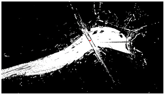
Figure 1.
A viewshed with a highlighted center point.
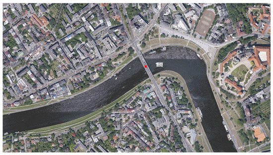
Figure 2.
A orthophoto map with a highlighted center point.
One of the methods to create a viewshed is to place a point of light in the digital model that contains a model of terrain and its coverage. Then, the rendering with a dedicated algorithm is performed. It results in a raster image with the marked surfaces that are either visible or invisible from the point where the light is located. The method requires the use of a digital terrain model whose representation would be able to reflect and obscure the rays of light. The only representation that meets such a requirement is TIN (triangulated irregular network). The effectiveness of algorithms in the TIN model has been described by Floriani [24]). The TIN surface is created by combining points with the smart use of triangles [25]. Vertices of that surface are points that, connected by edges, create triangles. In the TIN representation, triangles constitute a continuous surface that can be both opaque and reflective to digital light rays.
Visibility can refer to all the objects visible from a given point or to surfaces from which a given point is visible. The former case is called active exposure, while the latter is called passive exposure [26]. To determine the visibility of large objects, one must compile viewsheds from many points distributed on the surface of the specific object [27]. Such viewsheds are arranged in monochrome maps on which the higher lightness value indicates that a larger part of the object is visible in a certain place. As concerns the analysis of the visibility of mountain ranges, lakes, or similar objects, the density of points spread on their surface is significant. To achieve suitable resolution of a visibility map, the number of points must be very large. Such data sets require a high computing power and memory.
The method of obtaining viewsheds that is believed to provide the best results in terms of quality is based on the use of a ray-tracing algorithm [8]. In that method, it is necessary to fill a space with objects that can obscure the rays of digital light. A perfect representation of 3D objects for that purpose is a polygon mesh defined on the TIN data. Since it is built on a digital terrain model and coverage from GIS layers, it requires moderate processing time. Therefore, a viewshed can be obtained relatively quickly. Point clouds acquired using LIDAR scanning contain much more detailed information about the area. A viewshed generated from that data would be much better analytical material. However, it was not possible to obtain models of TIN surfaces and polygon meshes for the analyzed area within an acceptable time. There are, nevertheless, some ways to optimize the process using segmentation of data and paralleling during the processing of the chunks of acquired data.
4. Radial Segmentation of Point Clouds
Because of the lack of access to the equipment able to convert the entire point cloud to a TIN surface in one go, it was necessary to split the point cloud into many smaller parts; this enabled the generation of the TIN surface within a predictable time. Then, the core of the innovative method was applied, i.e., the cloud was divided into radial parts with the center at the viewpoint. Such an approach was taken for a reason: The angle range of the view did not affect the visibility of individual objects in space. The speed of generating the TIN surface in the radial sections of the point cloud depends on the angular range that can be chosen freely. To obtain a full viewshed, one can combine TIN surfaces of all radial slices. However, it is more efficient to generate viewsheds on each of the sections separately. They should be combined together to create one image with the desired spatial extent. Figure 3 presents a fragment generated from the point cloud compared to an orthophoto map.
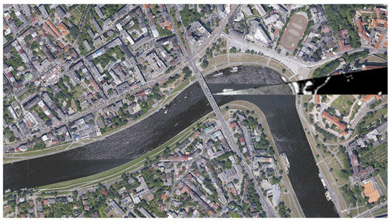
Figure 3.
A viewshed of the orthophoto map section with the highlighted center point.
The radial parts are determined by specifying the center point (viewpoint) of an area and then the minimum/maximum angles that are later used to construct a visibility cone. On the other hand, only the points that are within the range of the cone are selected for further calculations; all other points are rejected. Every single point must be checked and accepted or rejected from the given cone. Unfortunately, this is a long process because the points in the referred file are kept in the order they were created. Therefore, the process of creation of each fragment requires the analysis of the entire data set.
5. Binary Trees
In this section, one presents the method of reorganization of a point cloud with the use of binary trees. The important elements of binary trees are:
- Root—the starting element of the tree;
- Subtree—a tree being a part of the main tree;
- Node—one of the elements of the tree.
5.1. BST Tree—Binary Search Tree
One of the simplest examples of a tree structure is the BST (binary search tree, Figure 4) [28]. It is a structure that retains the rules of sorting and storing. The left subtree includes the points that have lower values than the root, whereas the right subtree includes the points with the higher values than the root. Each node of the subtree becomes a root for another set of subtree points. Turning the storage structure of point cloud into a binary tree enables the possibility of optimizing the processing time of point cloud data.
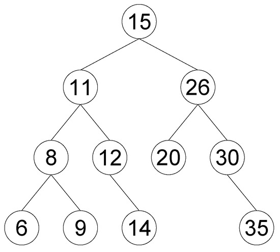
Figure 4.
An example of a binary tree.
One of the reasons for using a binary tree in the point cloud is to sort the points according to their distance from the selected central point. In this case, tree nodes can be represented by the distance between the current point and the central point after projecting them on the XY plane. The limitation of the point cloud size can be performed by rejecting points that are too far from the central point. The disadvantage of this solution is the necessity of creation of a separate BST tree for each central point.
Figure 5 presents a fragment of a point cloud with two distance ranges from the center point. If a binary tree structure is not used, each point should be checked by calculating its distance from the central point individually. With the use of a binary tree, all points within the chosen range can be selected in an easy and quick way.
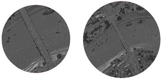
Figure 5.
An example of two ranges of distance from the central point.
The program execution time is proportional to the size of the cloud stored in the tree. However, when one wants to perform an operation for another range, creating a binary tree and checking the distance to points, which is the most time-consuming step, can be omitted. Avoiding the repetition of binary tree construction can reduce the range determination time.
Unfortunately, a separate tree must be created for each central point. Hence, the main problem remains unsolved.
5.2. k-d Tree
The k-d tree is another type of binary tree [28]. In the field of IT studies, it is referred to as a k-dimensional tree. Creating this type of tree is not complicated. The process consists in dividing the point cloud seen as a set of multiple tree nodes, each of which divides the points into subsets. The division is made according to the axes (in the case of two-dimensional trees) or by planes (in the case of three-dimensional trees). The points on the left side represent the left subtree, whereas the points on the right represent the right subtree. The order in which the divisions are made depends on the choice of the median according to the axes or planes. In other words, if one creates a 2D tree, the division follows the alternating X-axis and the Y-axis. In general, the dimension of the k-d tree is not predetermined; 2D or 3D trees, etc. are allowed. Trees are generated for the whole cloud. This results in the possibility of choosing any point as the central point of division, which was not provided by the BST. The selection of the k-d tree also gives the opportunity to apply many methods of paralleling the process of generating radial slices for different angles, which speeds up the work on the entire cloud. Figure 6a–d presents the process of k-d tree creation.
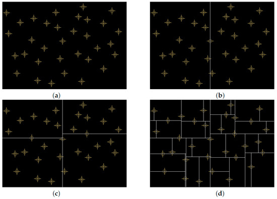
Figure 6.
(a) An exemplary point cloud is projected onto the XY plane. (b) A point cloud divided by a vertical axis passing through a point in the median defined along the X axis. (c) Subsequent division according to the points in the medians for the left and right subtrees after the Y axis. (d) Repeat previous steps for all subtrees.
A point cloud is projected onto the XY plane. (b) A point cloud divided by a vertical axis passing through the median point defined along the X axis. (c) Subsequent divisions according to the median points for the left and right subtrees, determined along the Y axis. (d) Repetition of previous steps for all subtrees.
The described example applies to a 2D tree. Figure 7 presents a case of a 3D tree that divides space using planes parallel to the main planes of the coordinate system.
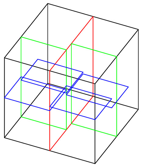
Figure 7.
A three-dimensional k-d tree.
6. The Subtree Rejection Algorithm in k-d Tree
The use of the k-d tree structure without using some additional accelerating algorithm does not trigger speeding up the division of the point cloud into radial parts. However, this very structure facilitates limiting the sets of points subjected to radial segmentation.
As previously indicated, the input data are a point cloud (set of points) that contains information about coordinates, brightness, and color. The goal of this study was to select the radial segment from the point cloud in the cylindrical coordinate system (Figure 8). The fragments are arranged on the XY plane; the Z coordinate is not taken into account. The structure of the cloud is redefined as a k-d tree, with only X and Y coordinates taken into consideration during the creation of a 2D tree.
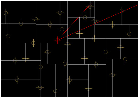
Figure 8.
A point cloud with the selected 2D-tree division axes with a specific point of the radial center, along with 30 and 50 degrees split directions.
To divide the point clouds into radial slices, it is advisable to approach them in narrow ranges. Then, the minimum and maximum directional angle vectors are close to each other, which means that large parts of the space do not have to be considered at all. Rejection of points that do not intersect the area between minimum and maximum directional angle vectors greatly accelerates the algorithm for determining slices. Depending on where the slice is pointing, there are different rules for rejecting subtrees that contain unnecessary points. The algorithm proposed in this paper formulates the rules according to which the key data points used to determine subtree rejection are special corner points located on the intersections of the k-d tree division axes. Description of the subtrees rejection algorithm. If the minimum and maximum area-limiting angles are between 0 and 90 degrees, all the points that are below the horizontal k-d tree division axis (A) (which is lower than the radial division point) are discarded. All points that are on the left from the vertical division axis of k-d tree (2), located on the left from this point (Figure 9), are discarded as well. Rejecting the next subtree marked green (Figure 9) requires checking if its left upper corner (1B) does not fall within the scope of the section. The coordinates of the 1B point result from the X coordinate of the axis 1 dividing the tree into the right and left part and from the Y coordinate of the B axis, dividing the right subtree into the upper and lower part. If the angle between the radial center point and point 1B is not in the section range, all points to the right of the axis (1) and down from the axis (B) can be rejected.
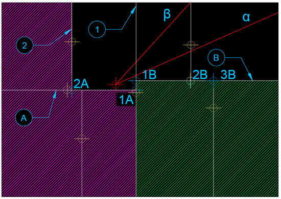
Figure 9.
Rejecting the subtrees.
Subsequent corners cannot limit the tree because they do not meet the rules for rejecting subtrees that are described in Section 6.1.1. According to Figure 9, it can be seen that the set of points which could belong to the radial section has been limited.
The rejected subtrees according to the above principles in the main tree are shown in Figure 10.
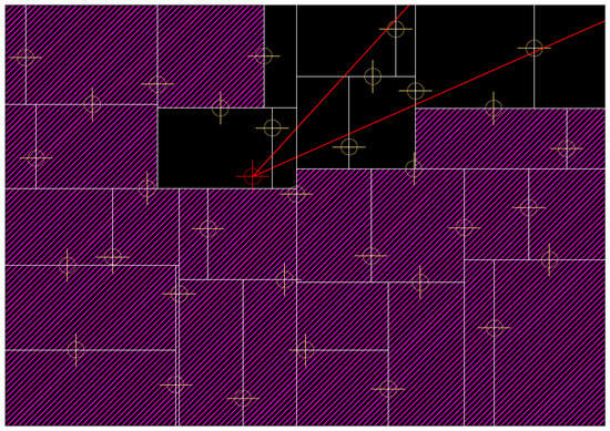
Figure 10.
All rejected subtrees.
An interesting case is a subtree marked in red in Figure 11. At first glance, it would be ideal for rejection, because it is completely out of the angular range of the radial segment. However, the indicated subtree was determined by the corner marked in blue and, therefore, referring to the description of the elements from Section 6.1, it is the left point. On the basis of subtree rejection rules, such a subtree cannot be rejected despite the fact that this would actually limit the number of points checked.
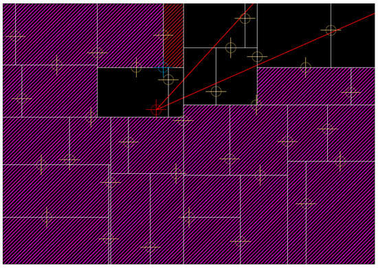
Figure 11.
An example of a not rejected subtree.
6.1. Description of Subtree Rejection Rules
The rules for describing points and angles should be adopted before discussing the rejection principles (Section 6.1.1). The following list shows points and angles with the specific names referring to their location (Figure 9).
- Point 1A belongs to the left subtree resulting from the division through axis 1; the point is located on the right side of the left subtree, and as a result, it was described as the RIGHT point;
- Point 1B belongs to the right subtree resulting from division by axis 1; the point is located on the left side of the right subtree, and as a result, it has been described as the LEFT point;
- Point 2B belongs to the upper subtree resulting from division by the B-axis; the point is located at the bottom of the upper subtree, and as a result, it was described as LOWER;
- Point 3B belongs to the lower subtree resulting from the division by the B-axis; the point is located on the top of the lower subtree, as a result of which, it has been described as UPPER;
- The angle LA0 is the angle between the straight line determined by taken point (this is one of the points: left—L (xl, yl), right—R (xr, yr), bottom—D (xb, yb), upper—G (xu, yu)) and the central point C and the axis OX;
- The MIN— angle is the angle LA0 with the lower value;
- The MAX— angle is the angle LA0 with the higher value;
- The red point is the central point of the division C—xc, yc.
For different angular intervals, there are different rules for rejecting a subtree. One of them is presented below. All of them are presented in the supplementary files.
6.1.1. Rules for 0–90 Degrees
- If the angle to the LEFT point is smaller than the MIN angle, reject the lower subtree.∀ (xl,yl) : 0 <LA0 < <90 reject {(x,y) : x ≥ xl; y ≤ yl}
- If the angle to the RIGHT point is greater than the MAX angle, reject the upper subtree.∀ (xr,yr) : 90 >LA0 > >0 reject {(x,y) : x ≤ xr; y ≥ yr}
- If the angle to the UPPER point is smaller than the MIN angle, reject the right subtree.∀ (xu,yu) : 0 <LA0 < <90 reject { (x,y) : x ≤ xu; y ≤ yu}
- If the angle to the BOTTOM point is greater than the MAX angle, reject the left subtree.∀ (xb,yb) : 90 >LA0 > >0 reject { (x,y) : x ≤ xb; y ≥ yb}
7. Results
Table 1 presents a comparison of radial slice generation times based on one degree angle and five degrees angle using different generation methods. Three methods of selecting points from the cloud for radial slices were compared: point by point, creating the k-d tree along with checking the angles in the k-d tree, and checking the angles in the k-d tree together with the subtree rejection algorithm. In these two methods, one has to additionally consider the time required to load all points into the computer’s memory and the time to generate a k-d tree. The comparison was made on four different point clouds of the same type, i.e., point clouds of all or parts of cities. In all cases, the cloud density remains the same. The following figures show a comparison of times for generating one radial slice with one degree angle (Figure 12) and time for generating ninety slices based on one degree angle (Figure 13). The presented charts show very accurately that for a single segment, the algorithm does not accelerate the generation of the slice. This is due to a large amount of time spent on generating a k-d tree. It is only during creating many slices that time decreases significantly. The next graph (Figure 14) shows the time needed to generate more slices. As indicated earlier, it is easy to notice that for individual slices, the times for k-d tree and k-d tree with the algorithm are similar, but for a larger number of slices, the subtree rejection algorithm significantly speeds up the generation procedure. The results prove that changing the point structure only is not sufficient for achieving the maximum acceleration. It should be additionally provided with some algorithms that limit the number of points for calculations, such as the presented subtree rejection algorithm.

Table 1.
Comparison of times needed to determine the radial parts of different point clouds using different methods.
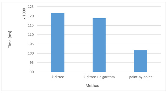
Figure 12.
The time needed to generate one slice based on one degree angle.
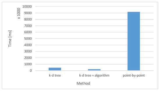
Figure 13.
The time needed to generate ninety slices every one degree.
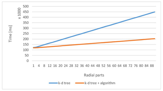
Figure 14.
Comparison of split times using only k-d trees and k-d trees together with the subtree rejection algorithm.
The time of performing the division into a radial section using k-d trees is presented together with the method of rejecting the subtree. The results depend on the direction and the point at which the division is made.
Specification of the computer which was used for research
- Processor i7-6820HQ CPU 2.70GHz
- 64 GB RAM
- Windows 10
Computational complexity of the algorithm
The determination of the angle between the point of observation and the corner resulting from the intersection of median lines in k-d tree was assumed as the leading operation. In a pessimistic scenario, for instance, when the whole cloud is included in the angular range, one will need to search all points in the grid, i.e., the complexity will amount to O (n). The actual calculation time depends on the real conditions (which will not always be the same) associated with the imposed pruning rules. Acceleration data are presented in Table 1.
8. Discussion
The presented results show a significant and large difference between the methods of creating viewsheds on the radial parts. If it is necessary to generate it on only one angle part, the presented algorithm does not speed up the search of points. This is due to the large time expenditure on loading points and creating k-d trees. However, the case of viewsheds on few radial parts is different. The construction of an algorithm to acquire these operations is based on the tree that is created once. Thus, the selection of points from it is very fast. In this case, the algorithm provides a very large acceleration in the acquisition of radial slices. Compared to the method where the points are searched point by point for many slices, the proposed algorithm accelerated this process several thousand times. In comparison with k-d tree not using the algorithm, it is still satisfying. In both cases, generating a k-d tree takes time. The use of k-d trees accelerates the process despite the need to check each point because the points are in the cache, but it is still long-lasting. Based on the above results, the algorithm finds its application with a greater number of slices. The acceleration that was obtained thanks to the rejecting subtrees algorithm in the k-d tree in comparison to the checking point by point reaches as much as 98%, and the k-d tree with the algorithm in relation to the same k-d tree 60%. Such significant acceleration can significantly support the processing of point clouds and their practical use. The resulting visibility charts can be used in many areas, such as urban planning, landscape research, security, visualizations or checking the accuracy and matching existing buildings to their digital models. There exist also algorithms for recognizing three-dimensional objects based on point clouds [29]. The point cloud itself can also store information on how points are allocated to different classes [22]. Presently, there are point clouds of the same elements or areas recorded over the years, which makes it possible to compare them and check for changes, i.e., occurring in the terrain or the impact of a given building or high voltage cable on the surrounding nature [30]. Therefore, point clouds can be used in many areas of research. The presented algorithm encourages their use by limiting the processing time. However, it should be noted that as shown in the presented charts, the algorithm accelerates operation only in the case of generating a number of radial slices. For individual slices, time is comparable to processing the cloud point by point. The presented article uses the k-d tree structure, which gives a large field of research for other types of structures that can further increase acceleration or globally change the time spent working on a point cloud. Such studies are already being carried out by the authors. The last, but also an important aspect, which provides an innovative method of rejecting subtrees is that in a flexible way, one can change the angular range of the generated slice, which does not require regeneration of a k-d tree.
9. Conclusions
This article presents the benefits of using binary trees to store and process a point cloud structure. One of the main benefits is the acceleration of point cloud searching and segmentation [31]. Additionally, a novel algorithm for rejecting the subtrees was proposed. The goal of the presented algorithm is to limit the number of points that are tested against its belongings to specific slices of radial segmentation which additionally accelerate the searching process. The obtained points are used to create viewshed and visibility maps. The algorithm execution time was presented in comparison to the time of performing the same operation without the use of k-d trees. Acceleration in accomplishing this particular task is several dozen times. The next step will be to distribute the algorithm by separating the subtree into different processors and threads, which will further accelerate the calculation process.
Supplementary Materials
The following are available online at https://www.mdpi.com/2073-8994/11/12/1451/s1, Description of subtree rejection rules.
Author Contributions
Conceptualization, J.O., P.O., and P.Ł.; Investigation, J.O.; Methodology, J.O.; Software, J.O.; Supervision, J.O.; Visualization, J.O.; Writing—original draft, J.O.; Writing—review and editing, P.O., P.Ł., A.W., and M.N.
Funding
This research received no external funding.
Acknowledgments
The authors would like to express their thanks to the editors for their helpful comments in advance.
Conflicts of Interest
The authors declare no conflict of interest.
References
- Prokos, A.; Kalisperakis, I.; Karras, G. Automatic point cloud generation and registration with a stereovision slit-scanner. In Proceedings of the 4th International Workshop on 3D Virtual Reconstruction & Visualization of Complex Architectures (3D-ARCH 2001), Trento, Italy, 2–5 March 2011; pp. 2–4. [Google Scholar]
- Su, J.; Srivastava, A.; Zhu, Z.; Huffer, F. Detecting Shapes in 2D Point Clouds Generated from Images. In Proceedings of the 20th International Conference on Pattern Recognition, ICPR 2010, Istanbul, Turkey, 23–26 August 2010. [Google Scholar]
- Blum, J.; Turner, K.J.; Winterbottom, Y. Cumulative Viewshed Analysis using GRID Computing (abstract of proposed paper for Geocomputation 2007). In Proceedings of the Geocomputation 2007, Maynooth, Ireland, 3–5 September 2007. [Google Scholar]
- Senaratne, H.; Bröring, A.; Schreck, T. Using Reverse Viewshed Analysis to Assess the Location Correctness of Visually Generated VGI. Trans. GIS 2013, 17, 369–386. [Google Scholar] [CrossRef]
- Cooper, G.R.J. Analysing potential field data using visibility. Comput. Geosci. 2005, 31, 877–881. [Google Scholar] [CrossRef]
- Nutsford, D.; Reitsma, F.; Pearson, A.L.K.S. Personalising the viewshed: Visibility analysis from the human perspective. Appl. Geogr. 2015, 62, 1–7. [Google Scholar] [CrossRef]
- Brabyn, L.; Mark, D.M. Using viewsheds, GIS, and a landscape classification to tag landscape photographs. Appl. Geogr. 2011, 31, 1115–1122. [Google Scholar] [CrossRef]
- Appel, A. Some Techniques for Shading Machine Renderings of Solids, SJCC Proceedings; Thompson Books: Washington, DC, USA, 1968; Volume 11, pp. 37–45. [Google Scholar]
- Ozimek, A.; Ozimek, P. Viewshed analyses as support for objective landscape assessment. J. Digit. Landsc. Archit. JoDLA 2017, 2, 190–197. [Google Scholar]
- Banaszek, L. Przeszłe krajobrazy w chmurze punktów; Wydawnictwo Naukowe UAM: Poznan, Poland, 2015. [Google Scholar]
- Han, X.F.; Jin, J.S.; Wang, M.J.; Jiang, W.; Gao, L.; Xiao, L. A review of algorithms for filtering the 3D point cloud. Signal Process. Image Commun. 2017, 57, 103–112. [Google Scholar] [CrossRef]
- Gressin, A.; Mallet, C.; David, N. Improving 3D Lidar point cloud registration using optimal neighborhood knowledge. In Proceedings of the ISPRS Annals of the Photogrammetry, Remote Sensing and Spatial Information Sciences, Melbourne, Australia, 25 August–1 September 2012; Volume I-3. [Google Scholar]
- Bustos, A.P.; Chin, T. Correspondence Rejection by Trilateration for 3D Point Cloud Registration. In Proceedings of the International Conference on Machine Vision Applications, Tokyo, Japan, 18–22 May 2015. [Google Scholar]
- Holz, D.; Ichim, E.I.; Tombari, R.; Rusu, R.B.; Behnke, S. Registration with the Point Cloud Library. IEEE Robot. Autom. Mag. 2015, 22, 110–124. [Google Scholar] [CrossRef]
- Mahmood, B.; Han, S. 3D Registration of Indoor Point Clouds for Augmented Reality. In Proceedings of the ASCE International Conference on Computing in Civil, Atlanta, GA, USA, 17–19 June 2019. [Google Scholar]
- Kim, Y.; Rana, S.; Wise, S. Exploring Multiple Viewshed Analysis Using Terrain Features and Optimisation Techniques. Comput. Geosci. 2004, 30, 1019–1032. [Google Scholar] [CrossRef]
- Caldwell, D.R.; Mineter, M.J.; Dowers, S.; Gittings, B.M. Analysis and Visualization of Visibility Surfaces (Poster). In Proceedings of the 7th International Conference on GeoComputation, Southampton, UK, 8–10 September 2003; University of Southampton: Southampton, UK, 2003. [Google Scholar]
- Orlof, J. Point Cloud based viewshed generation in Autocad Civil 3D. Tech. Trans. 2017, 12, 143–155. [Google Scholar]
- Las Specification; The American Society for Photogrammetry & Remote Sensing: Red Hook, NY, USA, 2019.
- Kurczyński, Z. Forogramertia; Wydawnictwo Naukowe PWN: Warszawa, Poland, 2014. [Google Scholar]
- Ptak, A. LiDAR w wielkim mieście. Geodeta: Magazyn Geoinformacyjny 2014, 12, 28–29. [Google Scholar]
- Orlof, J. Chmura punktów—nowa struktura danych. Aura ochrona środowiska 2017, 12, 3–6. [Google Scholar]
- Rubinowicz, P.; Czyńska, K. Study of City Landscape Heritage Using Lidar Data and 3d-City Models. In Proceedings of the International Archives of the Photogrammetry, Remote Sensing and Spatial Information Sciences, Kuala Lumpur, Malaysia, 28–30 October 2015; Volume XL-7/W3. [Google Scholar]
- Floriani, L.; Falcidieno, B.; Pienovi, C. Delaunay-based representation of surfaces defined over arbitrarily shaped domains. Comput. Vis. Graph. Image Process. 1985, 32, 127–140. [Google Scholar] [CrossRef]
- Floriani, L.; De Magillo, P. Visibility algorithms on triangulated digital terrain models. Int. J. Geogr. Inf. Syst. 1994, 8, 13–41. [Google Scholar] [CrossRef]
- Ozimek, A.; Ozimek, P.; Bohm, A.; Wańkowicz, W. Planowanie przestrzeni o wysokich walorach krajobrazowych przy użyciu cyfrowych analiz terenu wraz z oceną ekonomiczną; Wydawnistwo PK: Cracow, Poland, 2013. [Google Scholar]
- Davis, L.S.; Benedikt, M.L. Computational models of space: Isovists and isovist fields. Comput. Graph. Image Process. 1979, 11, 49–72. [Google Scholar] [CrossRef]
- Hanan, S. Foundations of Multidimensional and Metric Data Structures; Morgan Kaufmann Publishers: Burlington, MA, USA, 2006. [Google Scholar]
- Schnabel, R.; Wahl, R.; Klein, R. Shape Detection in Point Clouds; Universität Bonn: Bonn, Germany, 2006. [Google Scholar]
- Mémoli, F.; Sapiro, G. Comparing Point Clouds. In Proceedings of the Second Eurographics Symposium on Geometry Processing, Nice, France, 8–10 July 2004. [Google Scholar]
- Brostow, G.J.; Shotton, J.; Fauqueur, J.; Cipolla, R. Segmentation and recognition using structure from motion point clouds. In Proceedings of the ECCV, Marseille, France, 12–18 October 2008. [Google Scholar]
© 2019 by the authors. Licensee MDPI, Basel, Switzerland. This article is an open access article distributed under the terms and conditions of the Creative Commons Attribution (CC BY) license (http://creativecommons.org/licenses/by/4.0/).