Coupling System Dynamics and Mixed Cellular Automata for Carbon-Economic Optimization in Coastal Zones: A Multi-Scenario Simulation Under SSP-RCPs

Abstract

Rising greenhouse gas concentrations have exacerbated global warming, elevating the importance of land use and land cover (LULC) changes in achieving carbon neutrality. This is especially true in coastal areas, which face dual pressures from rapid urbanization and the need to protect carbon sinks. This study developed an SD-MCCA coupling framework to predict the dynamic changes in LULC in four SSP scenarios (SSP126, SSP245, SSP370, SSP585) in the coastal zone of Zhejiang Province from 2020 to 2100. Among them, the carbon storage was estimated by the InVEST model, and the dual-target optimization was carried out using the NSGA-II algorithm. Results indicated that construction land expanded significantly across all scenarios (50.3–110.2%), leading to a decline in carbon storage. However, outcomes were highly scenario-dependent; by 2100, carbon storage under the SSP126 pathway (1032.94 Mt) was notably higher than under the SSP585 pathway (1012.90 Mt). Coastal wetlands and forests emerged as major contributors to carbon storage, exhibiting high positive contribution scores, while construction land sites show significant negative correlations. Dual-target optimization achieved collaborative improvement: the optimized SSP126 scenario increased carbon storage by 1.16%, while economic benefits increased by 9.05%. The policy proposal emphasizes the priority of the SSP126 scenario, restricts the expansion of construction land, and enforces the ecological red line of wetlands and forests, guided by the phased Pareto optimal strategy.

1. Introduction

The acceleration of global warming caused by greenhouse gas emissions poses a serious threat to ecological safety [1]. In line with the Paris Agreement’s target of 1.5–2 °C, China is committed to peaking carbon emissions by 2030 and achieving carbon neutrality by 2060 [2]. LULC change is crucial in this work, because different types of land have different carbon fixation capabilities [3]. This is especially important in coastal areas, which face double pressures from rapid urbanization and the protection of important carbon sinks such as wetlands and forests [4]. Previous studies have confirmed the far-reaching impact of LULC changes on carbon storage: humans consume a quarter of the world’s land carbon storage [5], and China alone has lost 279 Tg of carbon storage (1980–2010), which is mainly caused by the expansion of farmland [6,7]. However, it is still a challenge to predict future dynamics under complex socio-economic and climate interactions.

Scenario prediction is widely used to assess the ecological impact of LULC and provide support for spatial planning [8,9,10,11,12,13,14]. However, most studies rely on traditional, single-dimensional scenarios (e.g., the continuation of trends) and lack a systematic link between socio-economic paths and climate policies. The SSP-RCP framework recognized by CMIP6 solves this problem by combining shared socio-economic pathways with representative concentration pathways [15,16]. Although recent studies have applied this framework to ecosystem services [17] and biomass carbon [18], significant gaps persist. First, comparative analyses of various coupling scenarios (e.g., SSP126 vs. SSP585) are typically insufficient to reveal interactive effects. Second, existing research is mainly focused on the global or national level; few studies can provide the high-resolution granularity required to solve the complex land–sea interactions unique to regional coastal planning. Third, existing forecasts often fail to integrate carbon storage and economic benefits into a unified multi-objective optimization framework, limiting their usefulness in a comprehensive trade-off analysis.

In order to solve these limitations, this study developed a coupled System Dynamics and Mixed Cellular Automata (SD-MCCA) framework integrated with NSGA-II multi-objective optimization. Unlike the traditional CA model constrained by the “pure cell” hypothesis, the MCCA method can accurately simulate the continuous proportional distribution of LULC types in the mixed landscape [19]. Beyond this spatial advantage, the framework introduces two further methodological advances over existing loosely coupled approaches: a closed-loop iterative coupling mechanism between SD and MCCA that ensures quantitative consistency between demand prediction and spatial allocation, and a spatially zoned optimization architecture in which NSGA-II operates on differentiated carbon management zones with zone-specific sensitivity coefficients, generating Pareto-optimal solutions that are directly actionable at the local level. Specifically, this study aims to: (1) simulate the dynamic changes in LULC in the coastal zone of Zhejiang under four SSP-RCP scenarios (2020–2100); (2) analyze the spatiotemporal evolution of carbon storage; (3) employ the NSGA-II algorithm to reconcile the conflict between development and conservation by identifying Pareto-optimal trade-offs, providing differentiated strategies for regional sustainable development.

2. Materials and Methods

2.1. Materials

2.1.1. Study Area

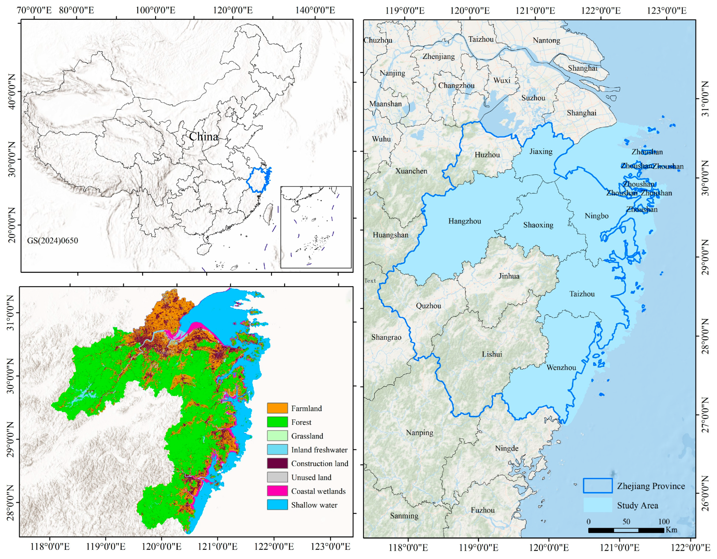
The coastal zone of Zhejiang Province (Figure 1) has a subtropical monsoon climate, with a coastline of about 6715 km. The study area is defined by the administrative boundaries of seven coastal cities (including Hangzhou and Ningbo) and extends seaward to the 10 m isobath, covering all provincial coastal wetlands.

2.1.2. Data Sources and Processing

Detailed information regarding the data used in this study is presented in

Table 1. Driver data source and processing.

Type	Year	Source	Method	Usage
LULC Data	2005, 2010, 2015, 2020	[20]	Landsat TM Satellite Image Classification	Input and validation data for SD and MCCA models
Population & Urbanization Rate	2020–2100	[21]	Recursive Multidimensional Model	SD model construction
GDP	2020–2100	[22]	Cobb–Douglas Economic Forecasting Model	SD model construction
Socio-economic Data	2005–2100	Zhejiang Statistical Yearbook (https://tjj.zj.gov.cn/col/col1525563/index.html, accessed on 1 July 2025)	Mathematical Statistics	SD model construction
Temperature and Precipitation	2020	Meteorological Data Station (https://data.cma.cn/, accessed on 1 July 2025)	Spatial Interpolation	Input data for MCCA model
DEM	2022	GEBCO (https://www.gebco.net/, accessed on 1 July 2025)	Acoustic Measurement, Gravity Inversion	Input data for MCCA model
Proximity to Roads	2022	National Geographic Information Service (https://www.webmap.cn, accessed on 1 July 2025)	Euclidean Distance	Input data for MCCA model
Proximity to Rivers	2022	National Geographic Information Service (https://www.webmap.cn, accessed on 1 July 2025)	Euclidean Distance	Input data for MCCA model
Proximity to Residential Areas	2022	National Geographic Information Service (https://www.webmap.cn, accessed on 1 July 2025)	Euclidean Distance	Input data for MCCA model
Proximity to Coastline	2020	[23]	Euclidean Distance	Input data for MCCA model
Future Climate Data	2020–2100	[24]	Downscaling and Bias Correction Techniques	SD model construction

.

1.

LULC Data

LULC data for the study area in 2005, 2010, 2015, and 2020 was obtained from an existing dataset [25]. The overall accuracy rate of this dataset is 80.88%, achieved through interpretation using Landsat grid imagery at a resolution of 30 m. This dataset employs a detailed classification system encompassing 35 LULC categories. The LULC types in this study are categorized into eight types: farmland, forest, grassland, inland freshwater, construction land, unused land, coastal wetlands, and shallow water.

2.

Socioeconomic Data and Future Scenario Data

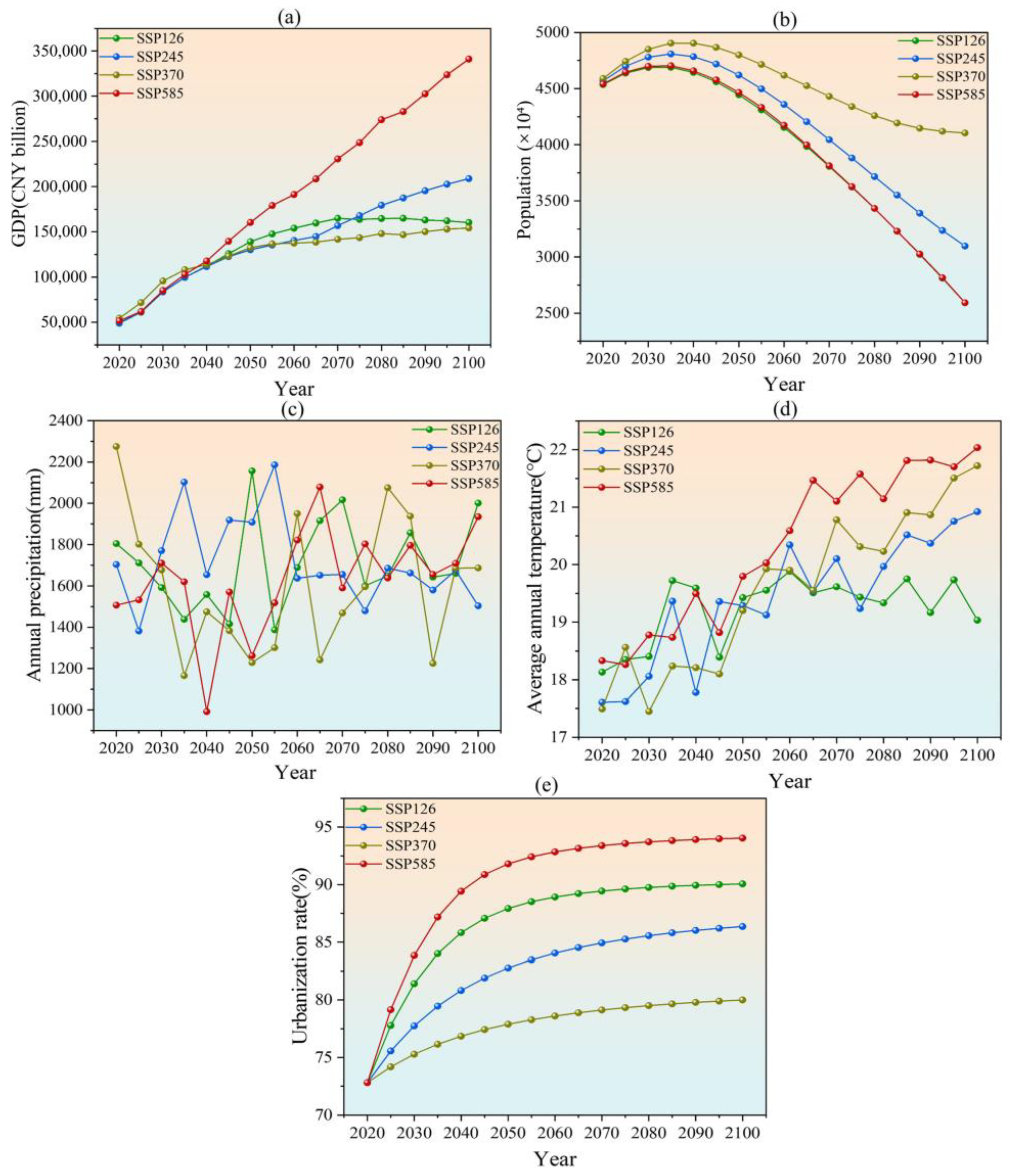
Population, urbanization rates, gross domestic product (GDP), fixed assets, and other socioeconomic data for historical periods were collected from the Zhejiang Statistical Yearbook and Bulletin from 2005 to 2020. Simulated data on population and urbanization rates for the future period are derived from existing projections [21]. This study selected population size and urbanization rate data for the study area under four scenarios: SSP126, SSP245, SSP370, and SSP585. The GDP data are sourced from the SSPs economic forecast dataset [22] publicly released by the Science Data Bank in 2022. This study assumes that the proportion of GDP contributed by each coastal city in Zhejiang Province to the provincial total will remain constant in the future. This proportion was multiplied by the simulated provincial GDP to generate multi-scenario GDP data for the study area spanning 2020 to 2100 (Figure 2a). Future climate data are derived from the High-resolution CMIP6 downscaled daily Climate Projections over China (HiCPC) dataset [24]. HiCPC represents China’s first high-resolution, daily climate projection dataset generated using CMIP6 global climate models and advanced downscaling and bias correction techniques (Figure 2c,d). This study processed daily data to generate annual data for four scenarios: SSP126, SSP245, SSP370, and SSP585 (Figure 2).

3.

LULC Driver Data

The selection of LULC drivers captures the combined effects of natural conditions, human activities, and coastal characteristics on LULC change. Drawing upon prior research [26,27] and considering data availability within the study area, this study selected temperature and precipitation as climate factors, and elevation as a topographic factor. Distances to transportation routes, settlements, and rivers were included as socioeconomic accessibility factors, and distance to coastlines as a coastal zone characteristic factor (Table 1). This factor system has been validated in coastal regions. A similar factor combination has been previously employed to simulate China’s coastal areas, achieving validation accuracy (Kappa coefficient) ranging from 0.803 to 0.939 [26]. This demonstrates the rationality and effectiveness of the selected factors. All spatial data are based on a 1 km resolution grid using the Krasovsky_1940_Albers projection coordinate system.

Figure 2. Trend Data for GDP (a), Population (b), Annual Precipitation (c), Annual Average Temperature (d), and Urbanization Rate (e) in the Zhejiang Coastal Zone, 2020–2100.

Figure 2. Trend Data for GDP (a), Population (b), Annual Precipitation (c), Annual Average Temperature (d), and Urbanization Rate (e) in the Zhejiang Coastal Zone, 2020–2100.

2.2. Research Framework and Methods

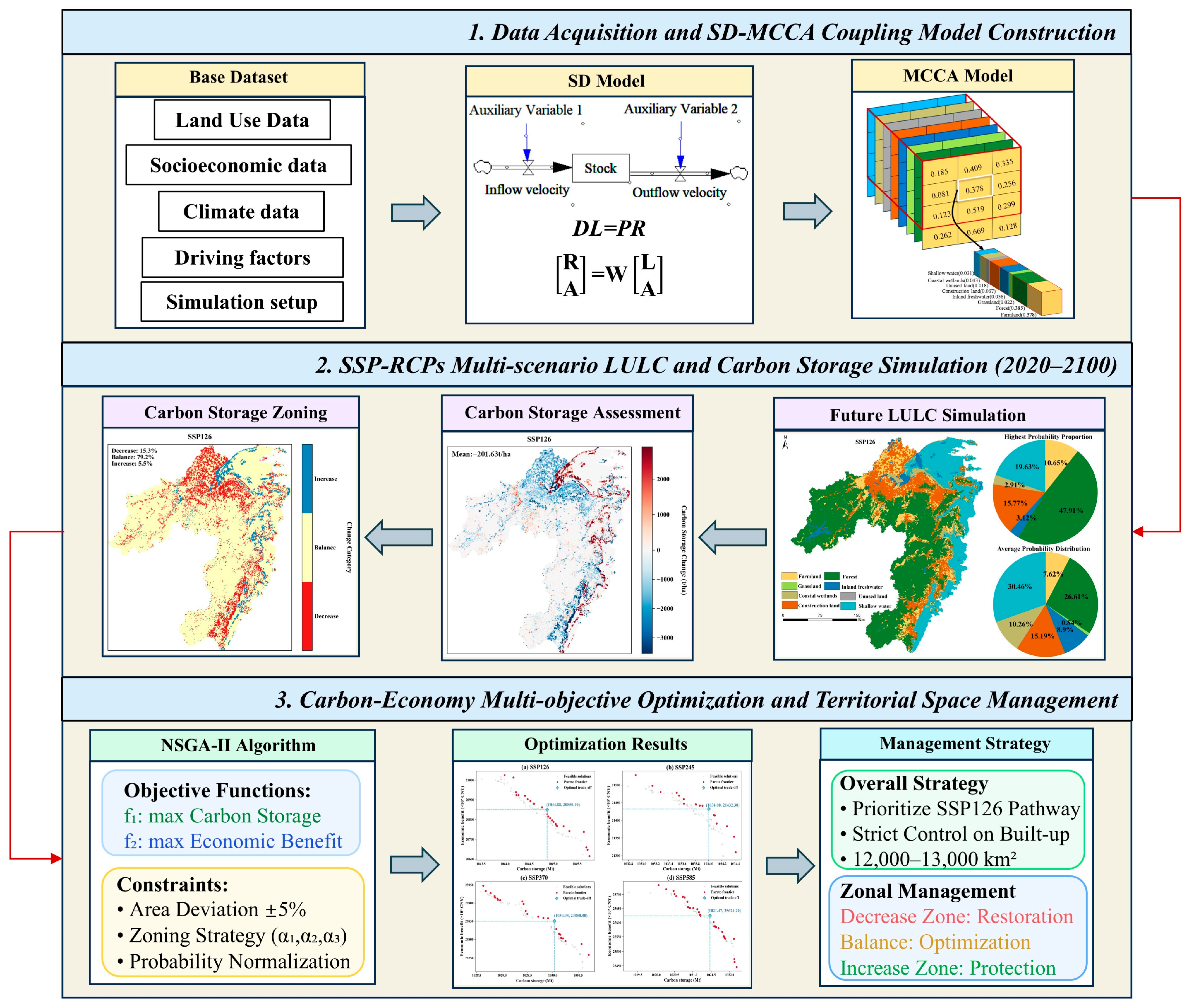
This study constructed an SD-MCCA-NSGA-II integrated framework to simulate LULC changes and carbon storage dynamics in the coastal zone of Zhejiang Province (Figure 3). First, the System Dynamics (SD) model integrates socioeconomic factors such as population, GDP, and urbanization rates to forecast land demand under four SSP scenarios. Second, the MCCA model employs a “mixed cell” structure to spatially allocate demand quantities. By integrating climate-adjusted carbon density data, it assesses carbon storage and identifies three management zones: carbon decrease zones, carbon balance zones, and carbon increase zones.

2.2.1. Construction of the SD-MCCA Coupling Model

This study constructed a coupled system dynamics and mixed cellular automaton model (SD-MCCA) to achieve simultaneous quantitative prediction and spatial configuration simulation of LULC change. The SD model forecasts the quantitative demand for various LULCs in the future, while the MCCA model translates this quantitative demand into spatial patterns. The coupling mechanism is as follows: the SD model’s scenario-specific LULC demand forecasts replace the linear regression and Markov chain methods conventionally used in CA models to derive historical and future land demand, serving as externally constrained area targets for the MCCA module. MCCA dynamically adjusts the simulated area through adaptive control coefficients, executing multiple rounds of iteration until the deviation from target demand falls below 5%.

• System Dynamics Model (SD)

An SD model was developed using Vensim^® PLE 8.1.0 (Ventana Systems, Harvard, MA, USA) to simulate LULC demand from 2005 to 2100 with a 5-year time step. The model comprised three interconnected subsystems. The socioeconomic subsystem incorporates population, GDP, urbanization rate, and fixed-asset investment as driving forces. The LULC subsystem models eight land categories (farmland, forest, grassland, inland freshwater, construction land, unused land, coastal wetlands, and shallow water) as stock variables with conversion flows regulated by socioeconomic demands. The policy regulation subsystem incorporates farmland, forest, and wetland protection intensities. The core feedback mechanism links population growth and economic development with the expansion of construction land, resulting in a decrease in farmland and ecological land, while policy interventions constrained the land conversion rate to balance development with ecological protection [28]. The data comes from the Statistical Yearbook of Zhejiang Province (2005–2020) and the Statistical Yearbook of Coastal Cities in Zhejiang Province. The model simulation comprised two stages [29]. First, the model was calibrated and validated using historical data from 2005 to 2020. Subsequently, scenario-specific parameters were derived from the SSP-RCPs database, and policy variables were adjusted according to each scenario’s narrative, generating LULC demands for SSP126, SSP245, SSP370, and SSP585 as quantity constraints for the MCCA model.

• Mixed Cellular Automata Model (MCCA)

The Mixed Cellular Automata (MCCA) model employs a “mixed cell” structure to represent the continuous proportional distribution of multiple LULC types within each cell [19]. It defines the state of each cell as a vector containing the coverage proportions of all LULC types (with the sum of proportions equaling 1). By utilizing a random forest regression method, it uncovers the quantitative relationship between changes in LULC proportions and driving factors, thereby predicting the growth potential of each LULC type within specific cells.

2.2.2. Future Scenario Setting

Scenario analysis is a method used to construct and interpret complex future scenarios [30,31]. Four scenarios were established based on the SSP-RCP framework to represent diverse socioeconomic and climate futures: SSP126 (Sustainable Development), SSP245 (Middle-of-the-Road), SSP370 (Regional Rivalry), and SSP585 (Fossil-fueled Development) [27,32]. These scenarios combine different levels of radiation forcing (RCP2.6 to RCP8.5) with different socio-economic development trajectories. Specific parameter settings regarding population, GDP, and policy constraints for each scenario are detailed in

Table 2. Parameter Settings for Different Development Scenarios.

Category	Variables	SSP126	SSP245	SSP370	SSP585
Dominant Variables	Population	Lower	Medium	High	Low
	GDP	Medium	Lower	Low	Higher
	Urbanization Rate	High	Medium	Lower	Higher
	Temperature	Lower	Medium	Higher	High
	Precipitation	Higher	High	Lower	Low
Trend Variables: Social Development	Per Capita Food Demand	High	Higher	Medium	Medium
	Water Resource Recycling	Higher	Low	Lower	Medium
	Fixed Asset Investment Ratio	Lower	Medium	Low	Higher
	Technological Progress	Higher	Lower	Medium	Higher
	Urban LULC Intensity	High	Medium	Lower	Low
	Mariculture Area	Lower	Medium	Low	High
	Coastal Tourist Numbers	Higher	Medium	Lower	Low
Trend Variables: Social Development Policy Protection	Farmland Protection Intensity	High	Medium	Lower	Low
	Forest Protection Intensity	High	Medium	Lower	Low
	Wetland Protection Intensity	High	Medium	Lower	Low
	Grassland Protection Intensity	High	Medium	Lower	Low

Note: The qualitative levels (Higher, High, Medium, Lower, Low) represent the relative magnitude of each variable across the four SSP scenarios, derived from the SSP-RCP narrative descriptions [15,16] and calibrated using provincial-level statistical data.

.

2.2.3. Carbon Storage Estimation

To quantify the impact of LULC changes on carbon storage under different SSP-RCP scenarios, this study required establishing quantitative conversion relationships between LULC types and carbon storage, enabling precise estimation of the spatiotemporal distribution of carbon storage from spatial patterns of LULC.

Carbon storage was estimated using the Carbon Storage module of the InVEST model (InVEST 3.18.0; Natural Capital Project, Stanford University, Stanford, CA, USA) [29,33]. The basic calculation formula for this module is shown in Equations (1) and (2). This formula was modified based on the mixed-cell characteristics simulated by MCCA, and the modified formula is presented in Equation (3).

$$C_i=C_{above}+C_{below}+C_{soil}+C_{dead}$$

(1)

$$C_{total}={\displaystyle \sum _{i=1}^n{A}_i}\times C_i$$

(2)

$$C_{total}={\displaystyle \sum _{i=1}^n{P}_{i,k}}\times C_i\times Are{a}_i$$

(3)

where $C_i$ denotes the total carbon density for LULC types $i$, $C_{above}$ denotes the above-ground biomass carbon density, $C_{below}$ denotes the below-ground biomass carbon density, $C_{soil}$ denotes the soil organic carbon density, and $C_{dead}$ denotes the litter carbon density. $C_{total}$ denotes the total carbon storage in the study area, $n$ represents the total number of LULC types, and $A_i$ is the area of LULC types $i$. Considering the probability distribution of each LULC type within mixed cells, the actual calculation of carbon storage employs a probability-weighted method. $P_{i,k}$ denotes the occurrence probability of LULC types $i$ in pixel $k$, and $Are{a}_i$ represents the area of a single pixel.

Biomass carbon density is closely related to climatic conditions [20,34]. Considering the impact of climatic variations across different regions on carbon density, this study employed the climate correction factor method proposed in [35], combined with previous research findings [36,37,38], to adjust the carbon density values for coastal zone in Zhejiang Province. Specifically, the effects of precipitation and temperature on biomass and soil carbon storage can be characterized by the following coefficients:

$$C_{SP}=3.3968\times MP+3996.1$$

(4)

$$C_{BP}=6.798\times e^{0.0054\times MP}$$

(5)

$$C_{BT}=28\times MT+398$$

(6)

where $C_{BP}$ and $C_{BT}$ denote biomass coefficients determined by precipitation and temperature; $C_{sp}$ denotes the soil coefficient determined by precipitation; $MP$ and $MT$ represent average precipitation (mm) and annual mean temperature (°C), respectively. Based on these impact coefficients, carbon density correction factors for vegetation and soil can be further developed:

$$K_{SP}={\displaystyle \frac{{C^{\prime }}_{SP}}{{C^{″}}_{SP}}}$$

(7)

$$K_{BP}={\displaystyle \frac{{C^{\prime }}_{BP}}{{C^{″}}_{BP}}}$$

(8)

$$K_{BT}={\displaystyle \frac{{C^{\prime }}_{BT}}{{C^{″}}_{BT}}}$$

(9)

$$K_B=K_{BP}\times K_{BT}$$

(10)

where $K_{BP}$ and $K_{BT}$ represent the vegetation carbon density correction coefficients derived from precipitation and temperature factors, respectively. Multiplying these two yields the vegetation carbon density correction coefficient $K_B$; $K_{SP}$ denotes the soil carbon density correction coefficient. Multiplying the obtained carbon density correction coefficients by the carbon density values collected from literature yields the corrected carbon density data for the coastal zone of Zhejiang Province. The carbon density data are presented in

Table 3. Calibrated carbon density parameters for different LULC types (Unit: t/ha).

LULC Type	${\mathit{C}}_{\mathit{a}\mathit{b}\mathit{o}\mathit{v}\mathit{e}}$	${\mathit{C}}_{\mathit{b}\mathit{e}\mathit{l}\mathit{o}\mathit{w}}$	${\mathit{C}}_{\mathit{s}\mathit{o}\mathit{i}\mathit{l}}$	${\mathit{C}}_{\mathit{d}\mathit{e}\mathit{a}\mathit{d}}$
Farmland	28.14	18.59	88.71	2.41
Forest	54.12	10.85	126.98	3.38
Grassland	25.91	31.03	112.29	2.92
Inland freshwater	0	0	83.53	0
Construction land	24.10	4.79	75.15	0
Unused land	36.20	7.27	79.99	2.22
Coastal wetlands	39.75	26.37	93.50	13.80
Shallow water	0	0	0	0

.

It is important to note that these climate-correction equations were applied solely to calibrate the baseline carbon density to local conditions. To isolate the specific contribution of LULC change to carbon storage dynamics, we assumed a static carbon density model where the carbon density values for each LULC type remain constant throughout the simulation period (2020–2100), independent of future climate fluctuations.

2.2.4. Multi-Objective Optimization of Carbon Storage and Economic Benefits

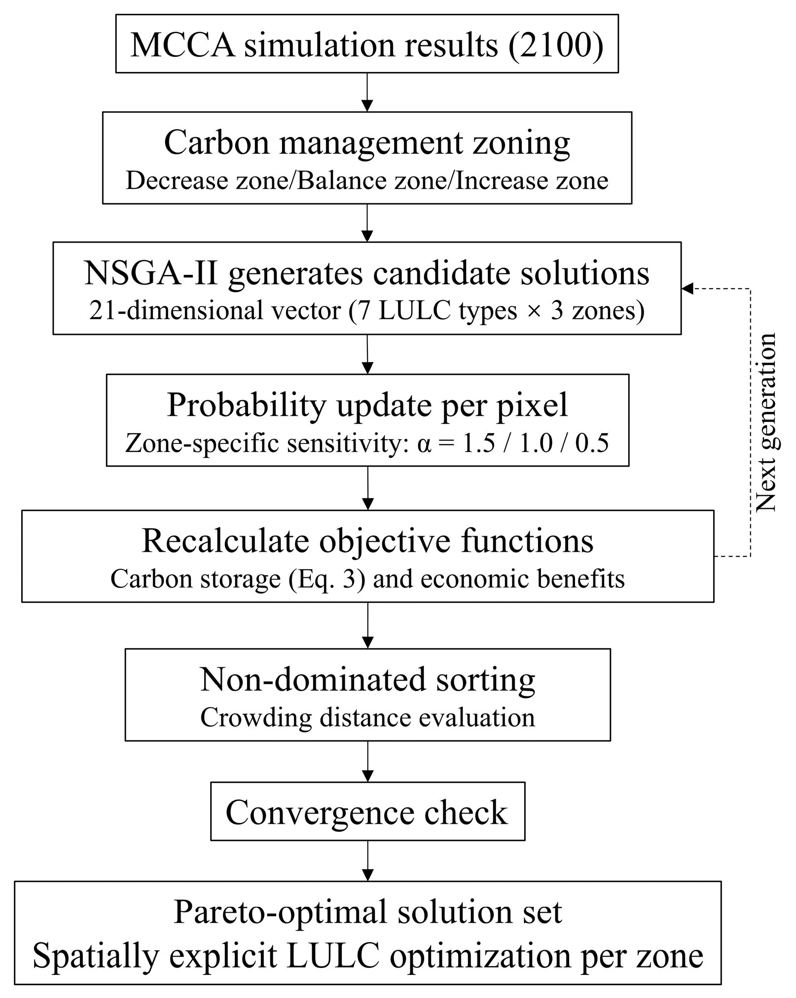
To identify optimal trade-offs between ecological conservation and economic development, this study employed the Non-Dominated Sorting Genetic Algorithm II (NSGA-II). This algorithm is widely recognized for its efficiency in handling non-linear, multi-objective problems by generating a diverse set of Pareto-optimal solutions [39]. The optimization operates on the MCCA simulation results at the terminal year (2100) for each SSP scenario. The overall workflow (Figure 4) first partitions the study area into three carbon management zones based on carbon storage change trends, then employs NSGA-II to iteratively search for zone-differentiated LULC adjustment strategies that simultaneously maximize carbon storage and economic benefits. The detailed formulations of the zoning scheme, decision variables, probability update mechanism, objective functions, and constraints are presented below.

• Decision Variable Design and Spatial Zoning

To address spatial heterogeneity, we adopted a partition-based optimization strategy. The study area was divided into three management zones ($z$) based on carbon storage trends: Carbon Decrease Zone ($z=1$), Carbon Balance Zone ($z=2$), and Carbon Increase Zone ($z=3$).

The decision variable is a chromosome vector $x\in {ℝ}^{21}$, representing the adjustment intensity for each of the seven LULC types ($j\in \{1,\dots ,7\}$) within each zone $z$. The vector is formulated as:

$$x=[x_{1,1},\dots ,x_{1,7},x_{2,1},\dots ,x_{2,7},x_{3,1},\dots ,x_{3,7}]$$

(11)

where the component $x_{z,j}\in [-1,1]$ represents the normalized adjustment magnitude for LULC type $j$ in zone $z$.

A Probability Update Mechanism was constructed to translate these macro-level adjustments into pixel-level probability changes. First, an intermediate unnormalized probability ${\tilde{P}}_{k,j}$ is calculated for each pixel $k$ located in zone $z$:

$${\tilde{P}}_{k,j}=P_{k,j}^0\times (1+x_{z,j}\cdot {\alpha }_z)$$

(12)

where $P_{k,j}^0$ is the baseline probability of LULC types $j$ at pixel $k$ in 2100 (derived from the SSP-RCP simulations), and ${\alpha }_z$ is the zoning sensitivity coefficient. To ensure valid probability distributions, a normalization operator is applied:

$$P_{k,j}(x)={\displaystyle \frac{{\tilde{P}}_{k,j}}{{\displaystyle \sum _{j=1}^7{\tilde{P}}_{k,j}}}}$$

(13)

This ensures that ${\displaystyle \sum _{j=1}^7{P}_{k,j}}(x)=1$ for every pixel. The sensitivity coefficients control how strongly the optimization can modify LULC probabilities in each zone. Higher values allow larger probability adjustments, enabling more aggressive intervention. We set $\alpha =1.5$ for Carbon Decrease Zones (allowing substantial redistribution to reverse carbon loss), $\alpha =1.0$ for Carbon Balance Zones (permitting moderate adjustment to optimize the existing structure), and $\alpha =0.5$ for Carbon Increase Zones (restricting changes to protect established high-storage configurations). These values were determined through preliminary sensitivity testing to ensure that the optimization produces meaningful but realistic adjustments within each zone.

• Objective Function

The optimization problem seeks to simultaneously maximize carbon storage ($f_1$) and economic benefits ($f_2$).

Objective 1: Maximize Carbon Storage

This objective aggregates the carbon stock of all grid cells based on the probability-weighted method:

$$f_1(x)={\displaystyle \sum _{k=1}^N{\displaystyle \sum _{j=1}^7{P}_{k,j}}}(x)\cdot C_j\cdot A_{grid}$$

(14)

where $N$ is the total number of pixels, $C_j$ is the carbon density (t/ha) for LULC type $j$ (Table 3), and $A_{grid}$ is the area of a single grid cell (1 km²).

Objective 2: Maximize Economic Benefits

This objective calculates the total economic value of ecosystem services and production:

$$f_2(x)={\displaystyle \sum _{k=1}^N{\displaystyle \sum _{j=1}^7{P}_{k,j}}}(x)\cdot E_j\cdot A_{grid}$$

(15)

where $E_j$ represents the unit economic value (10⁴ CNY/ha). The economic value parameters were derived from the Zhejiang Statistical Yearbook (2006–2021) and the China Marine Statistical Yearbook, deflated to 2005 constant prices using the GDP deflator to ensure cross-year comparability. The final unit economic values are: Construction land (142.54), Grassland (8.50), Inland freshwater (4.60), Farmland (4.20), Coastal wetlands (3.23), Forest (0.55), and Unused land (0).

• Constraints

To ensure the optimized solutions are realistic and compliant with macro-development scenarios, the following constraints are imposed:

Constraint 1: Probability Normalization

As defined in the probability update mechanism, the sum of LULC probabilities in any pixel $k$ must equal 1:

$${\displaystyle \sum _{j=1}^7{P}_{k,j}}(x)=1, \forall k\in \{1,\dots ,N\}$$

(16)

Constraint 2: Scenario Consistency (Area Targets)

The optimized LULC structure must not deviate significantly from the macro-demands predicted by the SD model for each SSP scenario. We set a tolerance threshold $ϵ$ = 5%:

$${\displaystyle \frac{|A_j(x)-A_j^{target}|}{A_j^{target}}}\le ϵ$$

(17)

where $A_j(x)={\displaystyle \sum _{k=1}^N{P}_{k,j}}(x)\cdot A_{grid}$ is the total optimized area for LULC types $j$, and $A_j^{target}$ is the scenario-specific demand. Solutions violating this constraint are penalized via a penalty function in the fitness evaluation.

3. Results

3.1. Performance Evaluation

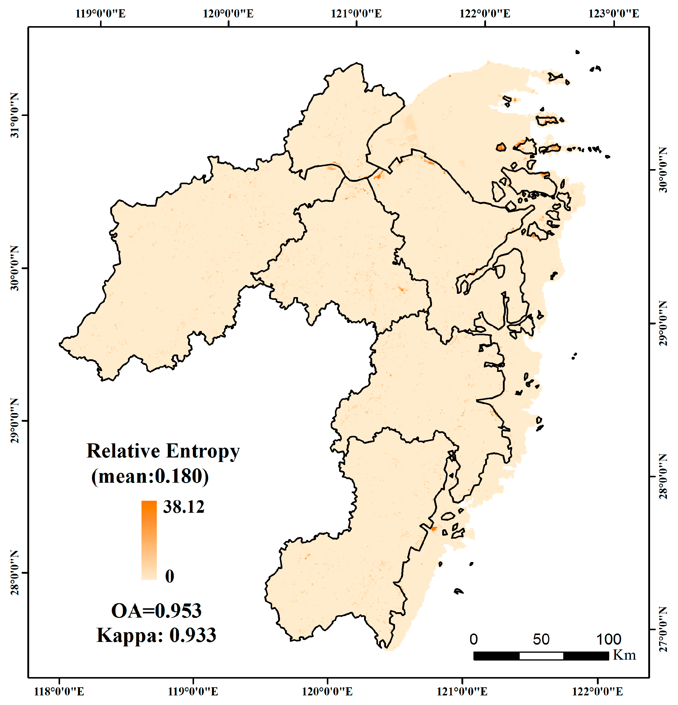
Comparing the 2020 simulation with actual observations validates the model’s reliability (Kappa = 0.933, OA = 0.953). Most land categories show relative errors within ±5.21% (

Table 4. Zhejiang Coastal Zone SD Model Error Values.

Year (2020)	Actual Value (km2)	Simulated Value (km2)	Relative Error (%)
Farmland	13,448.22	13,045.30	−2.99%
Forest	36,171.18	36,844.80	+1.86%
Grassland	25.0875	24.71	−1.50%
Inland freshwater	2663.28	2738.75	+2.83%
Construction land	8139.47	7715.72	−5.21%
Unused land	7.7949	17.85	+129.00%
Coastal wetlands	2223.88	2282.29	+2.63%
Shallow water	15,425.42	15,434.90	+0.06%

), which falls within the acceptable range established in previous studies [40]. Although “unused land” exhibited a high relative error (+129.00%), this was attributed to its extremely small base area (7.79 km², <0.02% of the total), which rendered it highly sensitive to minor pixel misallocations. Given its negligible role in carbon storage, this deviation does not compromise the study’s overall validity. Based on this foundation, using 2020 as the baseline year, LULC demand projections were generated for four scenarios extending to the year 2100, with data points generated every five years.

The average relative entropy (RE) serves as an indicator describing the similarity between the actual LULC structure and the simulated LULC structure across the entire study area. A lower RE value indicates greater similarity between the simulated and actual LULC structures. In most regions of the study area, the simulated structure closely resembles the actual structure. Areas with higher RE values are predominantly distributed in coastal wetlands and inland shallow water (Figure 5).

3.2. Forecast Results for Future LULC Demand

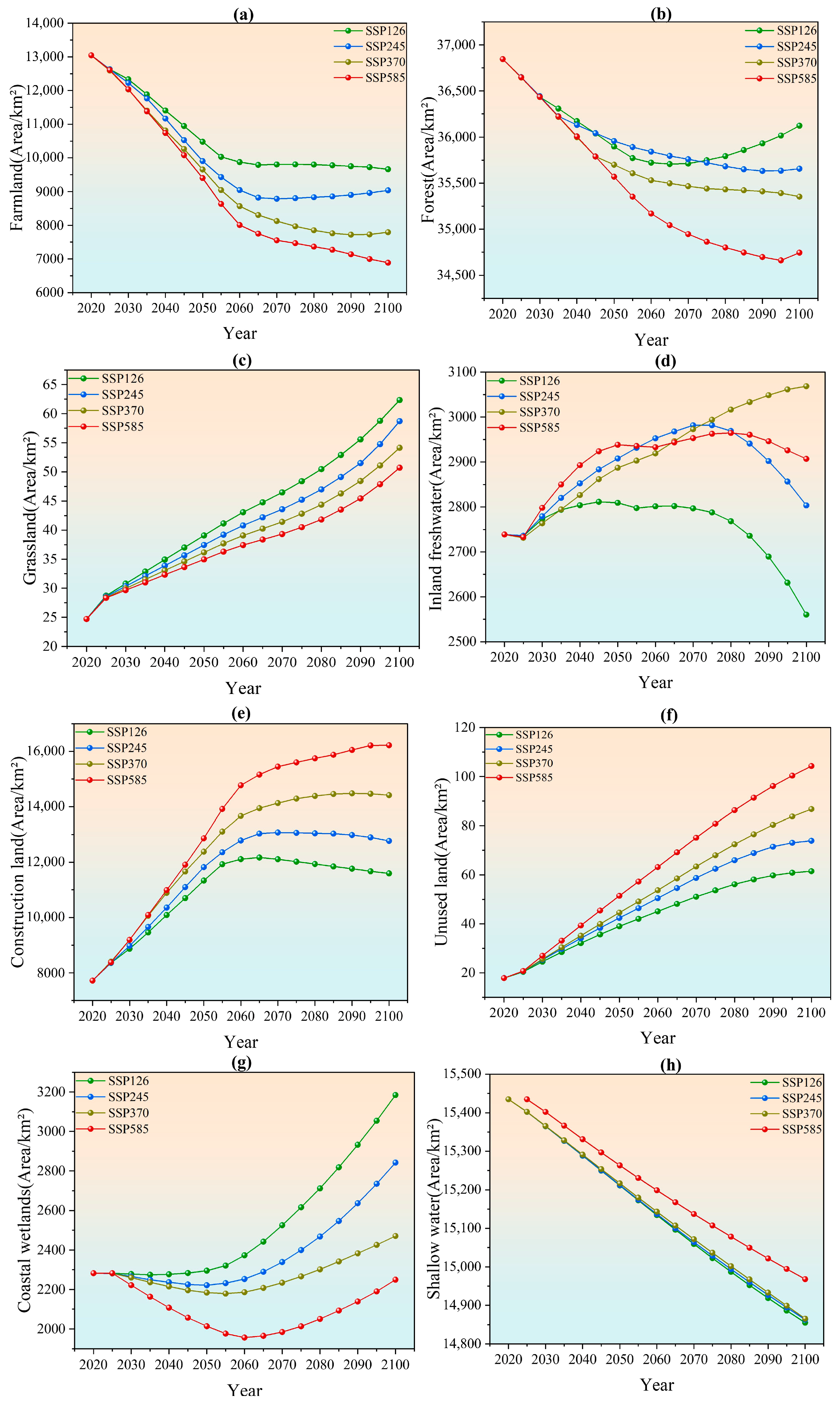
Based on the SSP-RCP scenario framework, this study simulated the projected changes in demand for major LULC types along the Zhejiang coast zone from 2020 to 2100 (Figure 6). Overall, farmland and shallow water areas show a persistent downward trend across all scenarios, while construction land exhibits a clear upward trend. The trends in coastal wetlands and forest vary significantly across scenarios. Grassland (Figure 6c), inland freshwater (Figure 6d), and unused land (Figure 6f) account for relatively small proportions of the study area and show minimal variation across scenarios; thus, they are not discussed in detail. The overall trajectory of LULC change is largely established in the short term (2020–2040), while differences between scenarios become pronounced in the medium to long term (2040–2100). Among all scenarios, SSP126 exhibits the most moderate changes with better preservation of ecological spaces, whereas SSP585 shows the most intensive encroachment on natural areas.

Construction land expands under all scenarios but with varying magnitudes (Figure 6e). While the sustainable SSP126 scenario successfully curbed growth to a moderate 50.3%, the fossil-fueled SSP585 scenario precipitated a drastic 110.2% surge, reflecting the intense land pressure inherent in high-energy development models. Notably, growth under SSP126 and SSP245 plateaus after 2070, indicating a transition toward intensive land utilization.

Farmland declines sharply in the short term across all scenarios (Figure 6a). By 2050, SSP585 will have the largest decline (27.9%), followed by SSP370 (24.6%), SSP245 (22.1%) and SSP126 (19.7%). In the medium and long term, the decline rate will slow down in all scenarios, while in the SSP126 scenario, the decline rate will tend to stabilize, which reflects the fundamental constraints of food security policies.

Changes in coastal wetlands directly reflect ecological conservation priorities (Figure 6g). Under SSP126, coastal wetland area increases to 3184.8 km² by 2100 (39.6% increase), while SSP245 reaches 2870.1 km² (25.8% increase), both demonstrating positive recovery trends. Conversely, under SSP370 and SSP585, although areas rebound after reaching their lowest points around 2040 (2156.3 km² and 2107.4 km² respectively), they fail to recover to baseline levels by century’s end. This pattern indicates that ecological losses caused by early intensive development are difficult to reverse without strong policy intervention.

Forest areas show distinct differentiation across scenarios (Figure 6b). Under SSP126, forest areas recover continuously after 2040, approaching baseline levels by 2100 (36,122.5 km²). SSP245 maintains relative stability (35,687.2 km²), while SSP370 declines slightly to 35,234.8 km². SSP585 exhibits the most significant decrease (34,856.1 km²). These differences correspond to varying levels of ecological protection investment across scenarios.

Shallow water areas exhibit a consistent linear decline across all scenarios (Figure 6h), with the rate of decrease strictly corresponding to development intensity (SSP585 > SSP370 > SSP245 > SSP126), primarily driven by coastal reclamation activities.

Figure 6. Simulation Results of Coastal Zone Land Demand Scenarios ((a–h) represent simulation results for farmland, forest, grassland, inland freshwater, construction land, unused land, coastal wetlands, and shallow water, respectively).

Figure 6. Simulation Results of Coastal Zone Land Demand Scenarios ((a–h) represent simulation results for farmland, forest, grassland, inland freshwater, construction land, unused land, coastal wetlands, and shallow water, respectively).

3.3. Spatial Simulation Results of LULC Under Multiple Scenarios

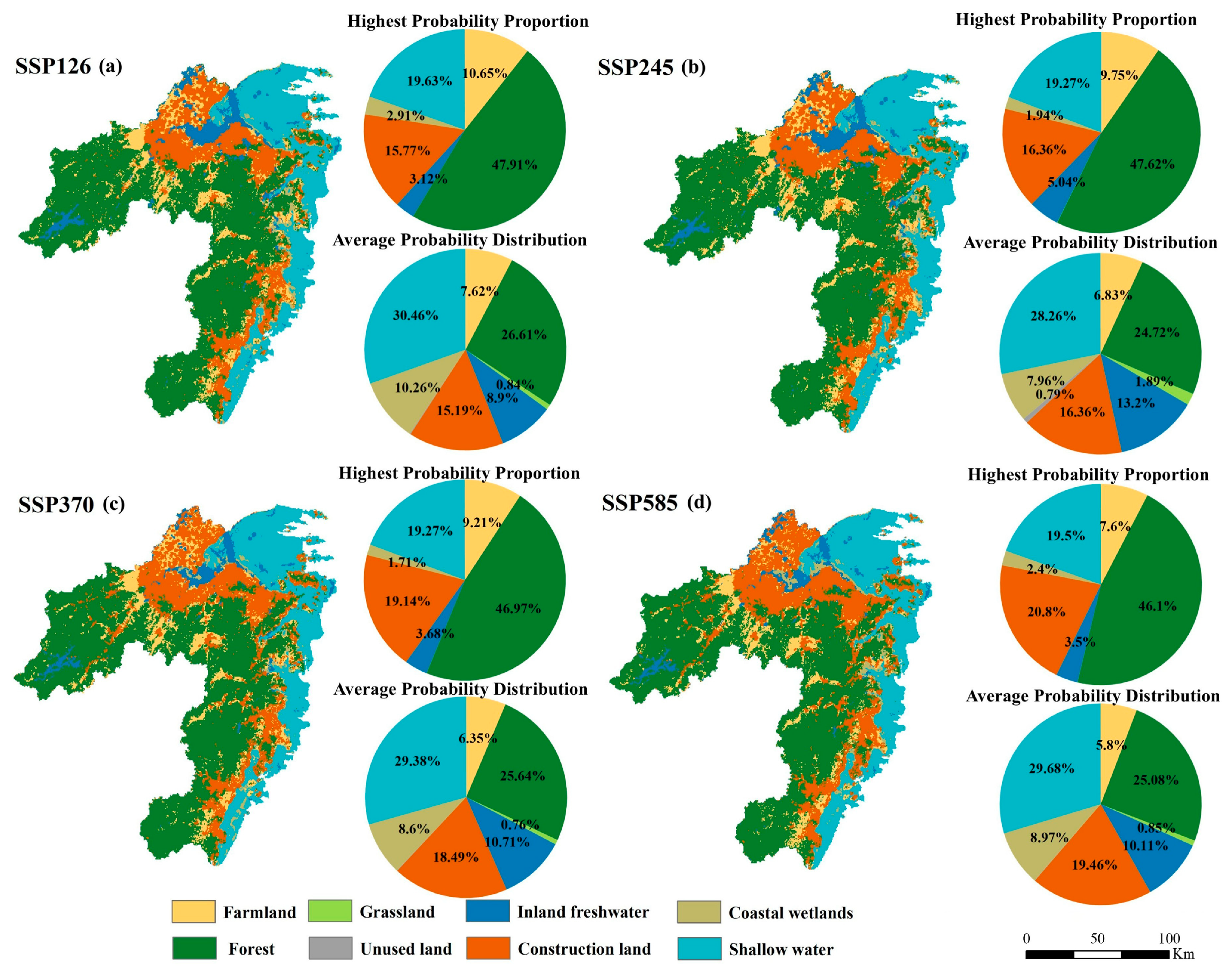
Based on the continuous LULC probability data predicted by MCCA, this study conducted spatial visualization primarily using the LULC type with the highest probability within each pixel (Figure 7). Results indicate that under various scenarios, the spatial structure of LULC types in Zhejiang Province will remain largely stable by 2100. This reflects the province’s distinctive geography characterized by predominantly mountainous terrain, with limited farmland and water bodies (often locally referred to as “seven parts mountains, one part water, and two parts farmland”) along with its terraced terrain sloping from southwest to northeast, extensive coastline, and numerous islands. Water bodies, unused land, and grasslands are sparsely distributed and structurally unstable. Construction land and farmland are primarily concentrated in the northern Zhejiang Plain and the southeastern coastal plains. Forested areas are clustered in the western hilly and mountainous regions, while coastal wetlands are concentrated at the land–sea interface along the coastline. The proportion of construction land varies most significantly across scenarios: SSP585 (Figure 7d) > SSP370 (Figure 7c) > SSP245 (Figure 7b) > SSP126 (Figure 7a). The smallest share occurs under SSP126, while the largest is observed in SSP585. Expansion is primarily concentrated in the northern Zhejiang plains, with relatively lower expansion in the southeastern coastal plains. The SSP126 pathway curbs construction land expansion, safeguarding farmland in alignment with sustainable development goals. Concurrently, the decrease in nearshore shallow water indicates a trend of construction land encroaching into shallow coastal waters. Shallow water areas and forest exhibit higher average proportions and pixel purity, indicating minimal disturbance. In contrast, farmland shows lower average probabilities, is susceptible to interference from other LULC types, and demonstrates pronounced spatial heterogeneity.

3.4. Carbon Storage Simulation Results Under Multiple Scenarios

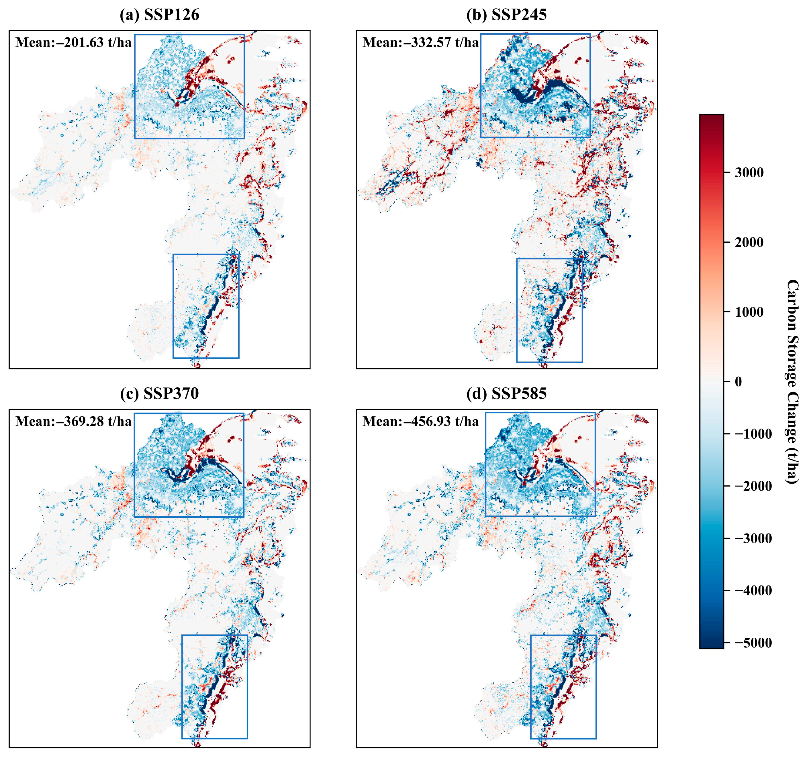
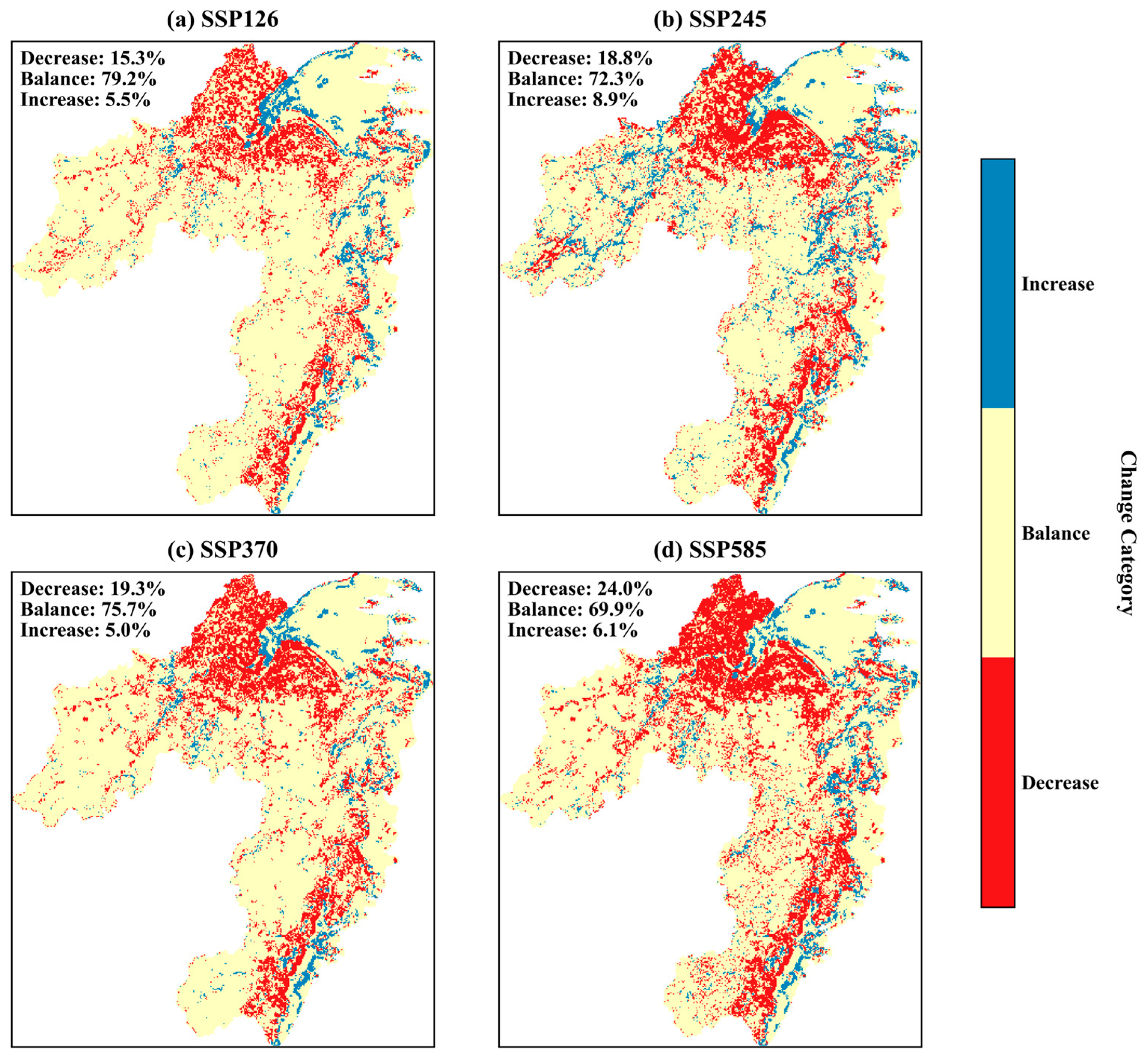
Regions with increasing and decreasing carbon storage are distributed throughout the coastal zone of Zhejiang Province (Figure 8). Among these, the Ning-Shao Plain and the Hang-Jia-Hu Plain have formed distinct clusters of reduced carbon storage (areas marked with blue boxes) due to the expansion of construction land, as observed across all scenarios. Under the SSP126 scenario (Figure 8a), stringent farmland protection policies restrict the conversion of farmland to forest, limiting carbon storage growth in certain regions. Under the scenarios of SSP370 (Figure 8c) and SSP585 (Figure 8d), this trend becomes more obvious. It is worth noting that the area with increased carbon storage under the SSP245 scenario (Figure 8b) is visually the most obvious. This was primarily because the SSP245 pathway represented an intermediate trajectory; it neither faced the strict farmland protection pressures of SSP126 nor experienced the rapid construction land expansion typical of SSP370 and SSP585. Consequently, it provides relatively favorable conditions for enhancing carbon storage. From a spatial distribution perspective, the areas experiencing increased carbon storage under all four scenarios are primarily concentrated in shallow coastal waters near the shoreline, driven mainly by the evolution of coastal wetlands. This is because the study area encompasses all categories of coastal wetlands within Zhejiang Province, a LULC type absent from other terrestrial ecosystems. Although the areal proportion of coastal wetlands is relatively small, their unit carbon density is notably high. Consequently, when other LULC types are converted to coastal wetlands, carbon storage increases accordingly. Coastal wetlands are recognized as highly efficient carbon sinks due to their capacity for long-term accumulation of sediments and organic carbon under anaerobic conditions [41]. Among these, the growth trend under the SSP126 scenario (Figure 8a) is most pronounced, particularly near Hangzhou Bay. In other scenarios, the southern shore of Hangzhou Bay has experienced varying degrees of carbon storage loss due to the expansion of construction land.

3.5. Carbon Storage Zoning Results Under Multiple Scenarios

A statistical method based on standard deviation thresholds was used to classify changes in carbon storage. The method calculated the standard deviation ($\sigma$) of carbon storage changes under each scenario for the period 2020–2100. Using 0.5σ as the threshold, the study area was classified into three categories: carbon decrease zones (change < −$0.5\sigma$), carbon balance zones ($-0.5\sigma$ ≤ change ≤ $0.5\sigma$), and carbon increase zones (change > $0.5\sigma$). This method can effectively identify areas of significant change while fully accounting for spatial heterogeneity across different scenarios.

The classification results show that under the SSP126 scenario (Figure 9a), carbon balance zones dominate, accounting for 79.2%. Under the SSP585 scenario (Figure 9d), carbon decrease zones have the highest proportion (24.0%). Under the SSP245 scenario (Figure 9b), carbon increase zones have the largest share (8.9%). Under the SSP370 scenario (Figure 9c), the proportion of carbon decrease zones (19.3%) is second only to that under the SSP585 scenario. Spatial distribution patterns exhibit distinct regional variations. Carbon decrease zones are primarily concentrated in urban expansion frontiers such as the Hangzhou-Jiaxing-Huzhou Plain and the southeastern coastal plains. Carbon balance zones exhibit the widest distribution, covering western mountainous regions, forested areas, and shallow coastal waters. Carbon increase zones occupy the smallest area, primarily occurring in scattered patches near coastal shallow waters and around inland freshwater (Figure 9).

3.6. Contribution of LULC to Carbon Storage

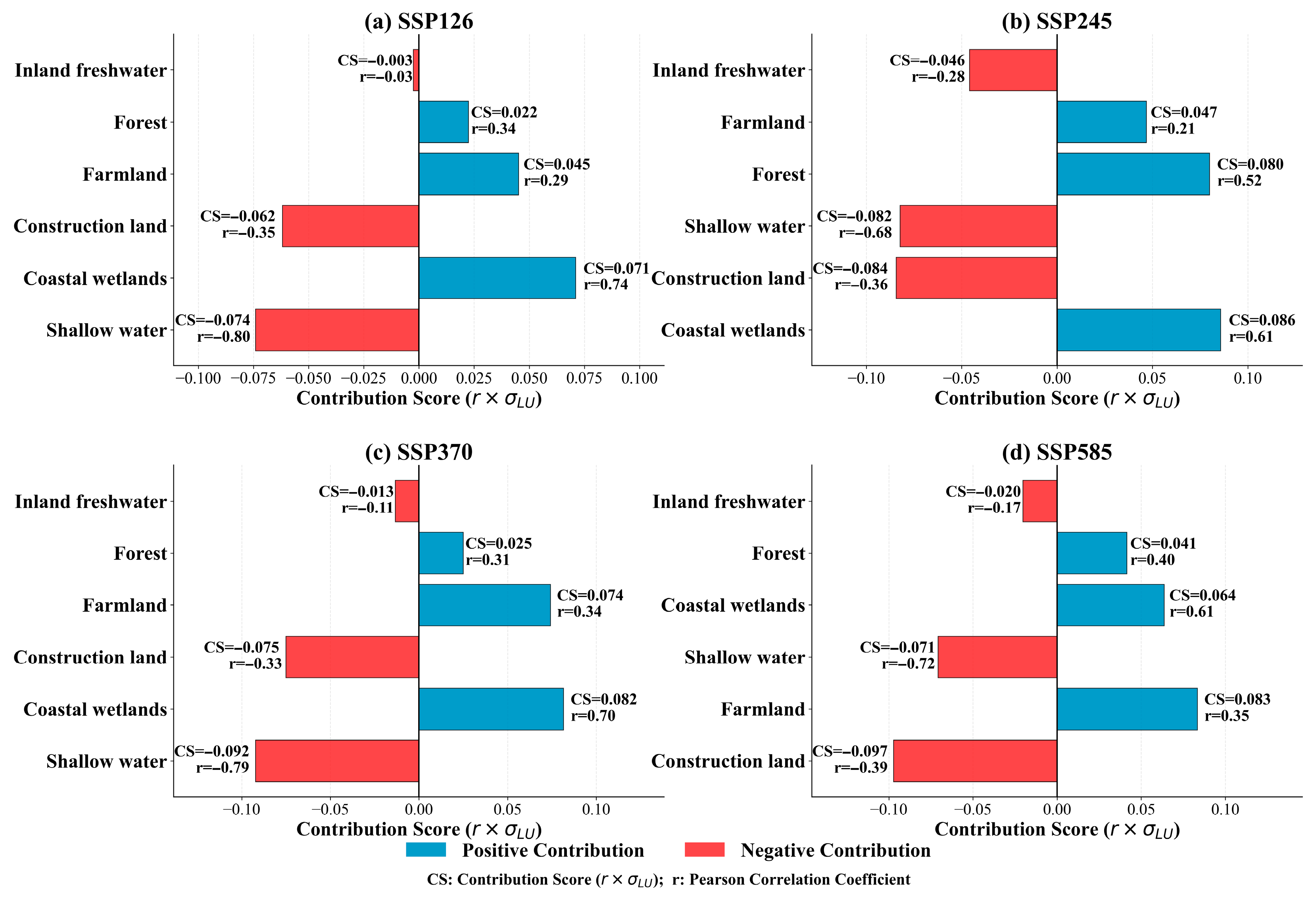
According to the contribution score analysis ($CS=r\times {\sigma }_{LU}$), coastal wetlands and farmland are identified as the main drivers of carbon increase in all scenarios (Figure 10). Specifically, as emission scenarios become more extreme, the contribution of farmland also increases (CS rises from 0.0452 in SSP126 to 0.0833 in SSP585; Figure 10a,d), which highlights the key role of agricultural management in extreme climatic conditions. On the contrary, shallow water areas and construction land have put continuous negative pressure on carbon storage. Although the shallow water area shows a strong negative correlation ($r\approx -0.80$), its actual contribution score varies greatly (Figure 10c), indicating that the correlation intensity and the degree of influence are not linear. While forests also contributed positively (peaking in SSP245; Figure 10b), their influence diminished in extreme scenarios, potentially reflecting climate stress constraints.

3.7. Characteristics of LULC Type Composition in Regions with Different Carbon Storage Changes

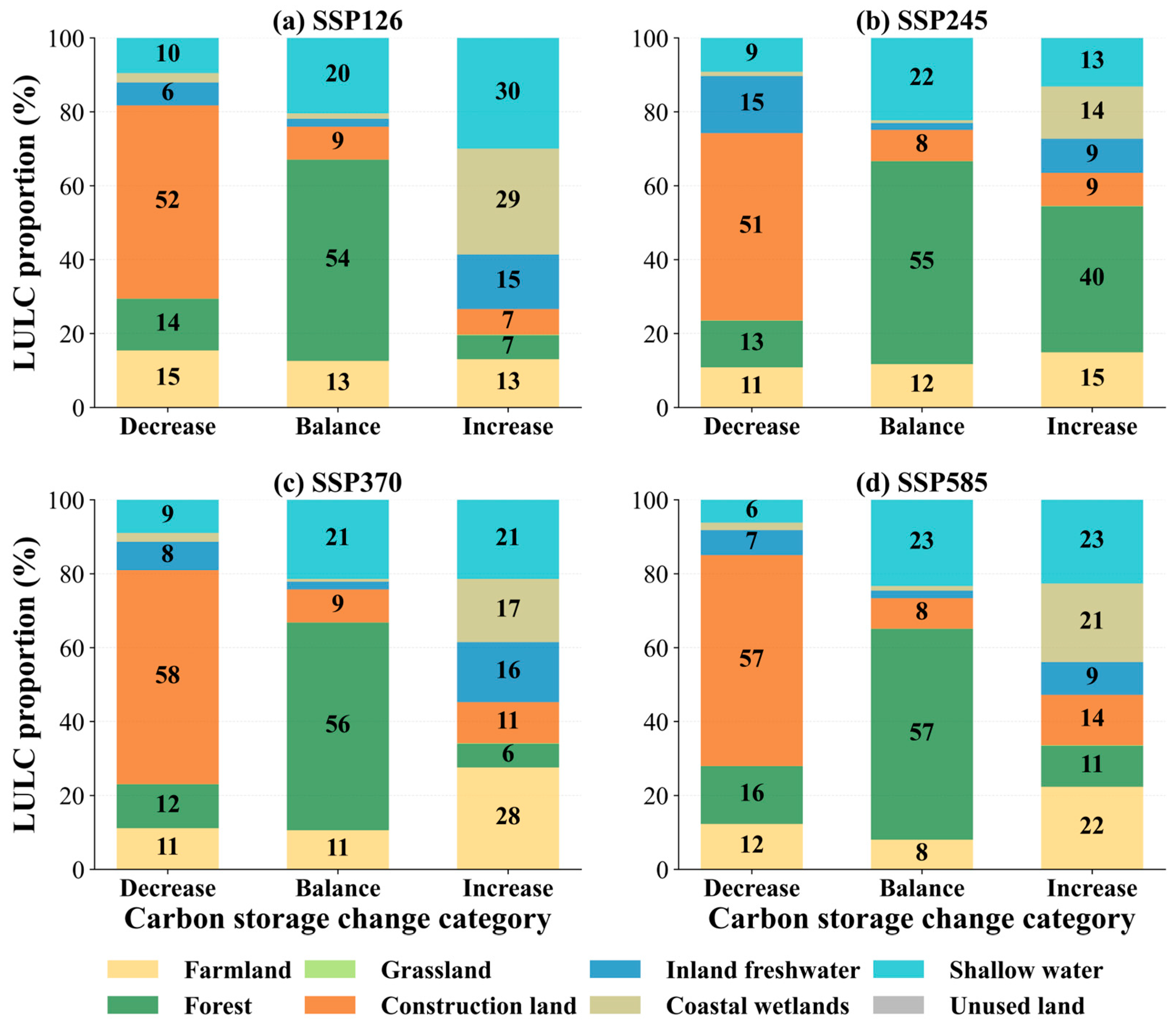
Under four different scenarios, the composition of LULC types across regions with varying carbon storage exhibits distinct spatial differentiation patterns (Figure 11). In regions with declining carbon storage, construction land dominates across all scenarios, accounting for 50.70–57.88%, followed by farmland (10.82–15.41%) and forest (11.92–15.63%). The high standard deviations (±39–45%) indicate considerable spatial heterogeneity within these regions. This composition suggests that urbanization and land development are the primary drivers of declining carbon storage.

In contrast, carbon storage balance regions are primarily characterized by forestry and agroforestry cover, which maintains a high proportion ranging from 54.46% to 57.08% across scenarios. Shallow water also contributes significantly (20.42–23.36%). The dominance of forestry and agroforestry in these regions underscores the critical role of forest ecosystems in maintaining regional carbon balance. Moreover, moderate pastoralism practices within and around forested areas can contribute to maintaining ecosystem health by reducing understory fuel loads, promoting vegetation heterogeneity, and enhancing nutrient cycling, thereby supporting the long-term carbon sequestration capacity of forest [42,43].

Regions with increasing carbon storage exhibit more heterogeneous LULC compositions with pronounced scenario-dependent variations. Under medium emission pathways (SSP126 and SSP245), these regions are characterized by higher proportions of coastal wetlands (28.61% and 14.15%; Figure 11a,b) and shallow water (30.01% and 13.13%; Figure 11a,b), reflecting enhanced carbon sequestration in aquatic and transitional ecosystems. Under stronger emission scenarios (SSP370 and SSP585), farmland becomes a major contributor (27.55% and 22.33%; Figure 11c,d), possibly reflecting enhanced agricultural management or vegetation restoration on degraded land. Coastal wetlands remain important carbon sinks across all scenarios.

Figure 11. LULC Distribution by Scenario in 2100 ((a) LULC distribution under SSP126 scenario, (b) LULC distribution under SSP245 scenario, (c) LULC distribution under SSP370 scenario, and (d) LULC distribution under SSP585 scenario).

Figure 11. LULC Distribution by Scenario in 2100 ((a) LULC distribution under SSP126 scenario, (b) LULC distribution under SSP245 scenario, (c) LULC distribution under SSP370 scenario, and (d) LULC distribution under SSP585 scenario).

3.8. Carbon Storage Status of Coastal Cities

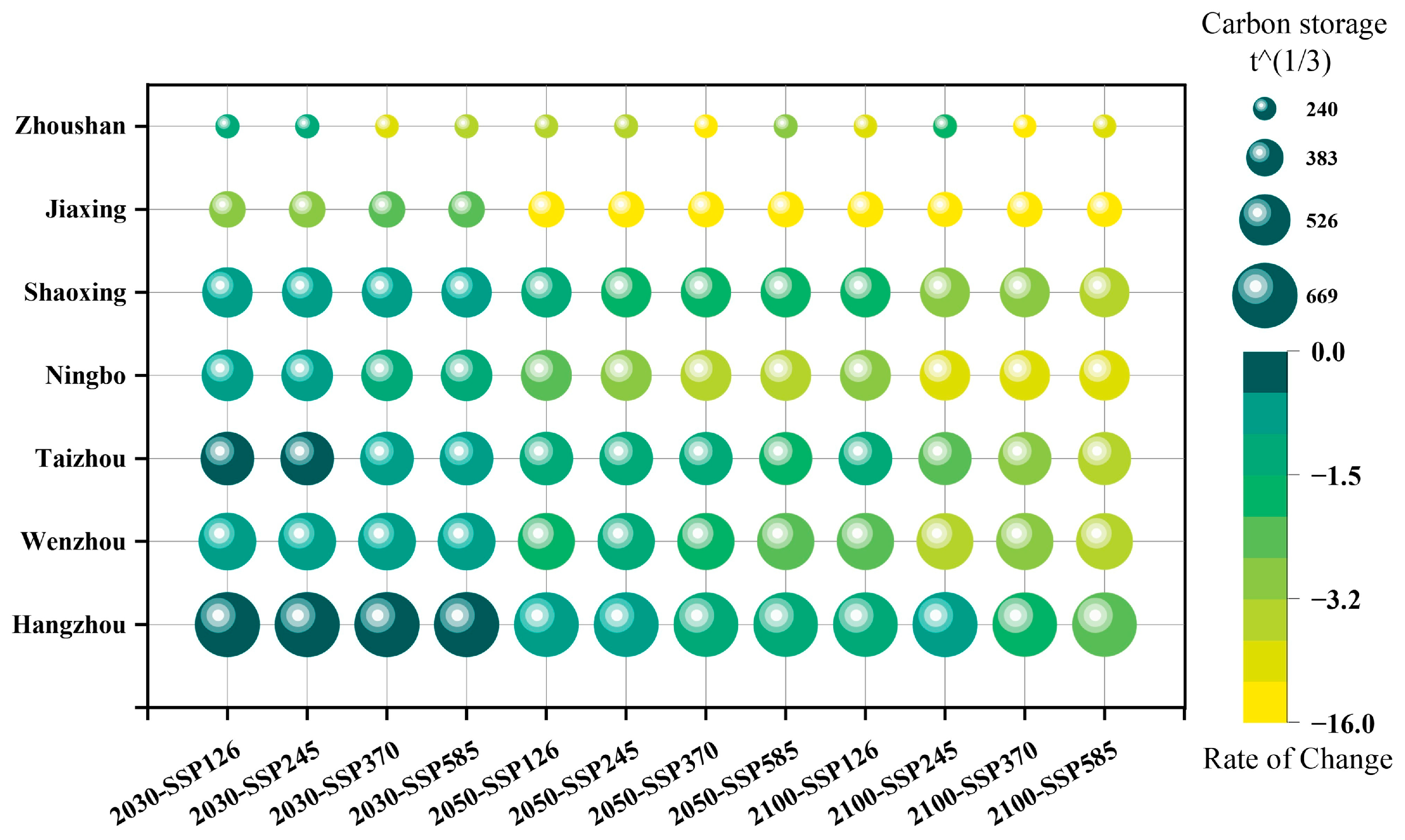
This study systematically assessed the trends in carbon storage changes across seven major coastal cities in Zhejiang Province under different scenarios (Figure 12). Results indicate that carbon storage in all cities will decline by 2100, with the rate of decline accelerating over time. Across all scenarios, the SSP585 pathway exhibits the most severe carbon decrease, while the SSP126 pathway shows the smallest relative decline.

In terms of carbon storage capacity, the overall ranking is Hangzhou (292.1 Mt) > Wenzhou (203.9 Mt) > Taizhou (164.7 Mt) > Ningbo (145.0 Mt) > Shaoxing (136.8 Mt) > Jiaxing (53.4 Mt) > Zhoushan (15.3 Mt). The order is roughly consistent with the land area of each city, but there are also obvious deviations. For example, the land area of Ningbo is comparable to that of Taizhou, but the carbon storage is low, which is mainly due to topographic differences: Taizhou is mainly mountainous (70.4% is low to medium mountainous and hilly), with high vegetation coverage, while the proportion of Ningbo Plain is higher (40.3%).

The analysis at the urban level reveals that there is an obvious topographic gradient in carbon resilience. Mountainous cities (e.g., Hangzhou, Wenzhou) maintain relatively stable carbon storage due to their vast ecological protected areas. In contrast, the decline in plain areas such as Jiaxing is the most serious (up to 15.66%), indicating that they are extremely vulnerable to the pressure of urban expansion. Characterized by flat terrain (88.8% plain) and a strategic location between Shanghai and Hangzhou, Jiaxing was particularly vulnerable to intense pressures from construction land expansion.

Figure 12. Carbon Storage Status of Coastal Cities in Zhejiang.

Figure 12. Carbon Storage Status of Coastal Cities in Zhejiang.

3.9. Dual-Objective Optimization Results for Carbon Storage and Economic Benefits

3.9.1. Dual-Objective Optimization Performance Across Four Scenarios

Based on the NSGA-II algorithm, this study optimized carbon storage and economic benefits in four scenarios. The optimization results show that all scenarios achieved synchronous growth of carbon storage and economic benefits, verifying the effectiveness of multi-objective optimization methods (

Table 5. Before and After Comparison of Four Scenario Optimizations.

Scenario	Phase	Carbon Storage (Mt)	Economic Benefit (×104 CNY)	Carbon Storage Increase	Economic Benefits Increase
SSP126	Before Opt	1032.94	19,119.43	-	-
	After Opt	1044.88	20,850.10	+1.16%	+9.05%
SSP245	Before Opt	1022.66	20,178.33	-	-
	After Opt	1034.00	21,432.30	+1.11%	+6.21%
SSP370	Before Opt	1019.78	22,462.34	-	-
	After Opt	1030.03	23,850.00	+1.01%	+6.18%
SSP585	Before Opt	1012.90	24,406.08	-	-
	After Opt	1021.47	25,624.20	+0.85%	+4.99%

Note: Opt = optimization.

).

3.9.2. Analysis of Differences Between Scenarios

1.

Characteristics of Carbon Storage Gradient

The initial carbon storage across the four scenarios exhibits a distinct gradient: SSP126 (1032.94 Mt) > SSP245 (1022.66 Mt) > SSP370 (1019.78 Mt) > SSP585 (1012.90 Mt), with a decrease of 20.04 Mt. This reflects the impact of LULC changes on carbon storage under different development paths. The low-carbon sustainable scenario (SSP126) maintains high carbon storage capacity by controlling the expansion of construction land and protecting ecological land. In contrast, the high-carbon development scenario (SSP585) has led to a sharp decline in carbon storage due to a significant increase in construction land (15,917.80 km², 31.3% more than SSP126).

The magnitude of optimized carbon storage increases also exhibits a gradient: SSP126 (+11.94 Mt) > SSP245 (+11.34 Mt) > SSP370 (+10.25 Mt) > SSP585 (+8.57 Mt). The relative enhancement rate decreased from 1.16% under the SSP126 scenario to 0.85% under the SSP585 scenario, indicating that the potential for carbon sink optimization is greater in low-carbon scenarios. This finding is negatively correlated with the proportion of carbon increase zones (15.3% under the SSP126 scenario and 24.0% under the SSP585 scenario).

2.

Characteristics of Economic Benefits Growth

The initial economic benefits show an inverse trend: SSP585 (24,406.08 × 10⁴ CNY) > SSP370 (22,462.34 × 10⁴ CNY) > SSP245 ((20,178.33 × 10⁴ CNY) > SSP126 (19,119.43 × 10⁴ CNY), with an increase of 27.6%. This is in line with the principle that the level of economic development is positively related to the proportion of construction land.

The optimized economic benefits improvement rate shows that SSP126 is the highest (9.05%) and SSP585 is the lowest (4.99%), demonstrating a “low base, high growth” pattern. This is because the construction land area designated in the SSP126 scenario is relatively small (12,124.10 km²), and it has greater potential to increase economic benefits through optimization and adjustment. Conversely, under the SSP585 scenario, construction land is close to saturation, and further expansion is limited by the area target (±5%).

3.

Scenario-Based Carbon Storage-Economic Trade-Off Relationship

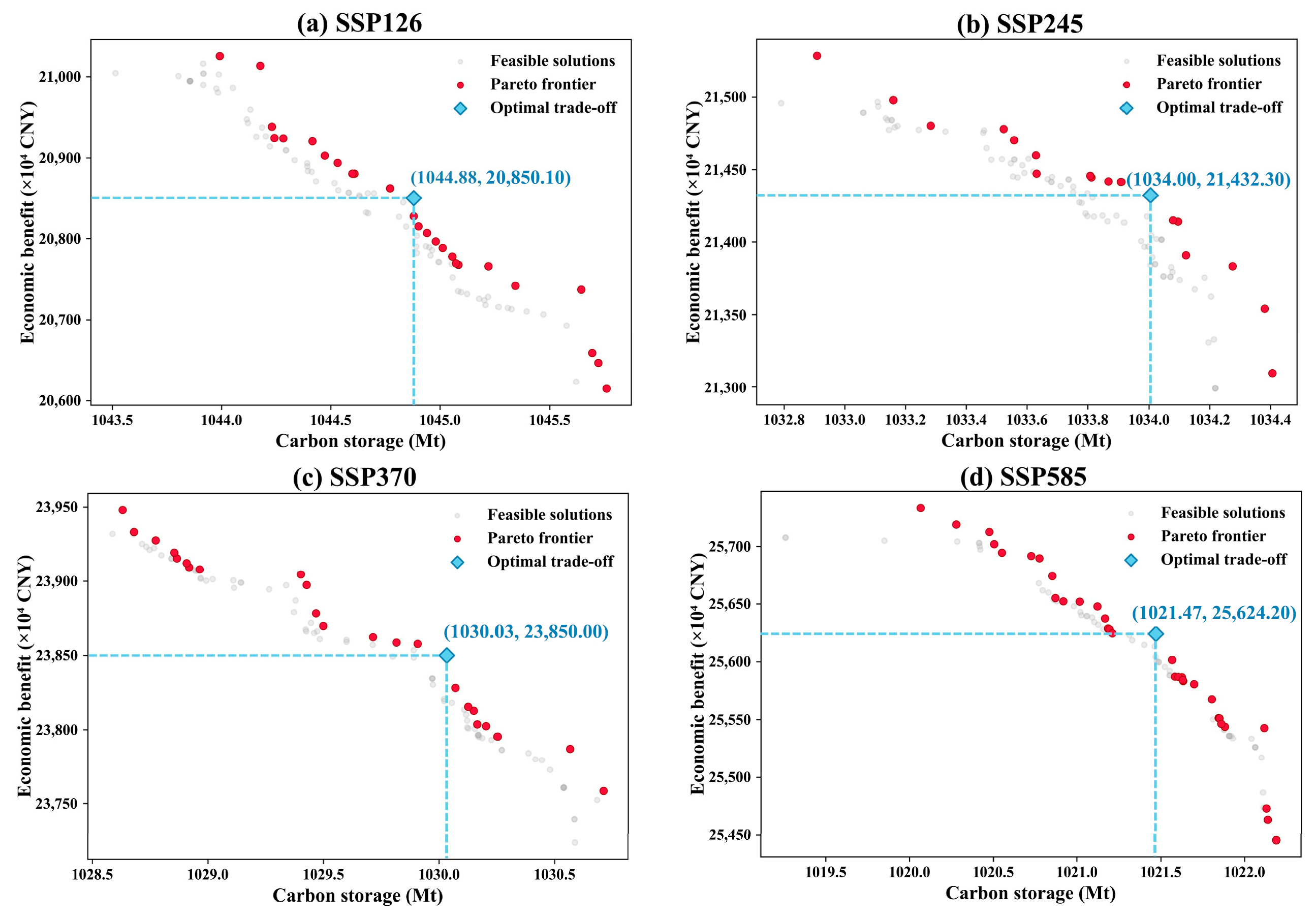
Optimal trade-off solutions (knee points) distribution for four scenarios (Figure 13):

• SSP126: Carbon 1044.88 Mt, Economic 20,850.10 × 10⁴ CNY (Figure 13a)
• SSP245: Carbon 1034.00 Mt, Economic 21,432.30 × 10⁴ CNY (Figure 13b)
• SSP370: Carbon 1030.03 Mt, Economic 23,850.00 × 10⁴ CNY (Figure 13c)
• SSP585: Carbon 1021.47 Mt, Economic 25,624.20 × 10⁴ CNY (Figure 13d)

Figure 13. Pareto Frontier Distribution Chart.

Figure 13. Pareto Frontier Distribution Chart.

3.9.3. Comparative Analysis of Spatial Partitioning Strategy Effectiveness

The statistics of carbon change zones (

Table 6. Four Scenario-Based Spatial Zoning Characteristics.

Scenario	Carbon Decrease Zone (%)	Carbon Balance Zone (%)	Carbon Increase Zone (%)	Threshold (Mt)
SSP126	15.3	79.2	5.5	±813.78
SSP245	18.8	72.3	8.9	±1218.17
SSP370	19.3	75.7	5.0	±1016.47
SSP585	24.0	69.9	6.1	±940.14

) reveal the significant spatial differences under different scenarios:

Scenario SSP585 has the highest proportion of carbon decrease zones (24.0%), mainly distributed at the forefront of urban expansion. Even if the adjustment range reaches the maximum value (${\alpha }_1=0.3$), the carbon increment still reaches 8.57 Mt, which shows that the differentiated spatial zoning strategy can effectively guide the ecological recovery of high-pressure areas. Scenario SSP245 has the highest proportion of carbon increase zones (8.9%). These areas adopt the smallest adjustment level (${\alpha }_3=0.1$) to avoid excessive intervention so as not to destroy the stable ecosystem.

In all four scenarios, the carbon balance zone dominates (69.9–79.2%). By applying a moderate adjustment level (${\alpha }_2=0.2$) to optimize the existing carbon economic balance, this method embodies the principle of balancing sustainable development and ecological protection in the management of national territorial space.

4. Discussion

4.1. Comparison of MCCA Model Based on Optimal Scale with Multi-Model Simulation Results

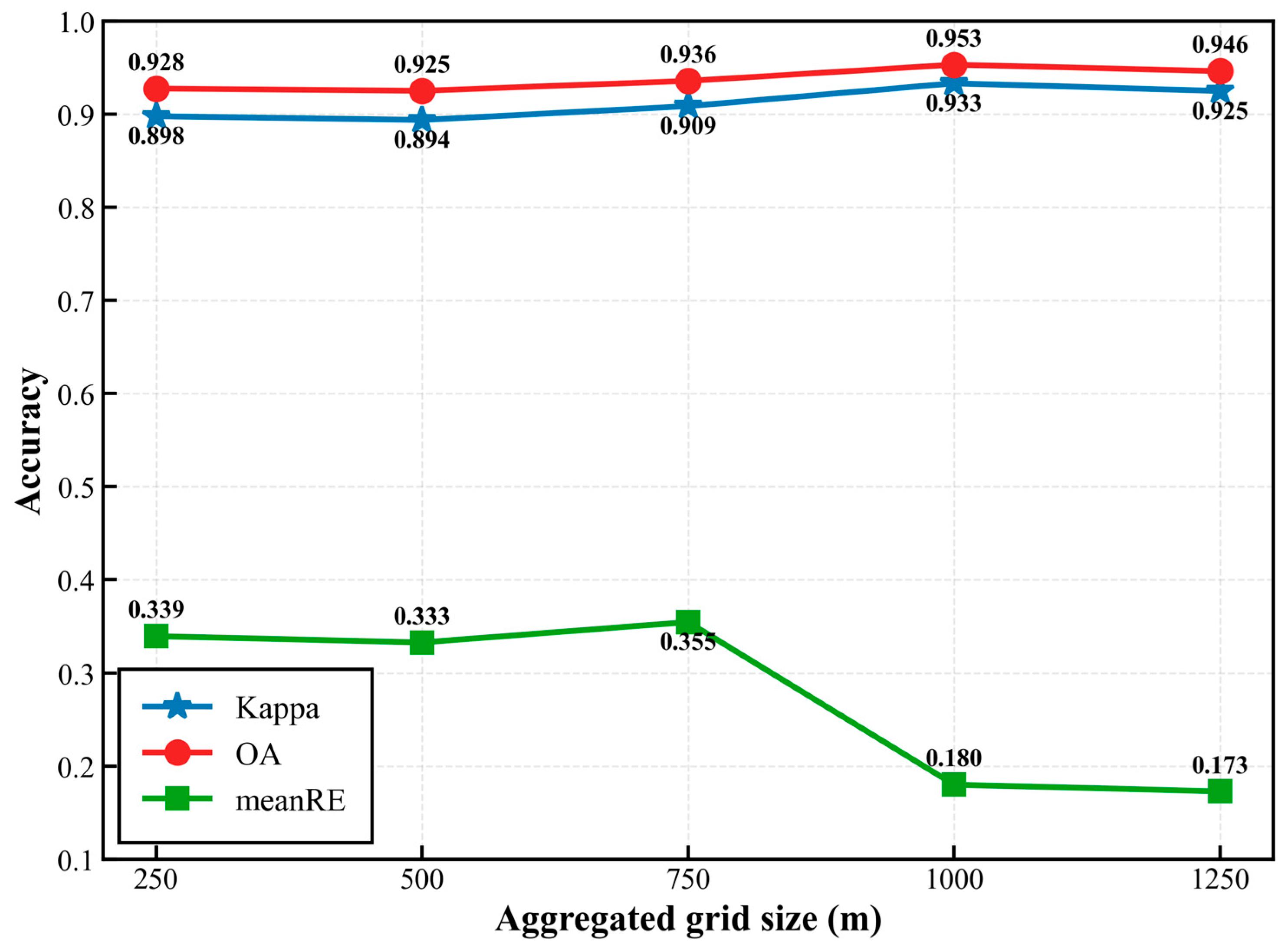
Sensitivity analysis shows that the grid scale affects the simulation accuracy, which is consistent with [19]. In this study, the 1 km grid scale was used, and the simulation accuracy was Kappa = 0.933 (Figure 14). In addition, the MCCA model is obviously superior to the traditional FLUS and PLUS models in capturing the fragmentation of the mixed landscape (Figure 14), verifying its superiority in the complex coastal transition zone. However, the optimal aggregation scale is not universally fixed but depends on the source data resolution and landscape heterogeneity of each study area, and should be determined through sensitivity analysis accordingly. Overall, the MCCA model is best positioned for meso- to macro-scale regions characterized by complex, heterogeneous LULC mosaics, and is not well suited for very fine-scale simulations where the aggregation process would obscure the spatial detail required for decision-making.

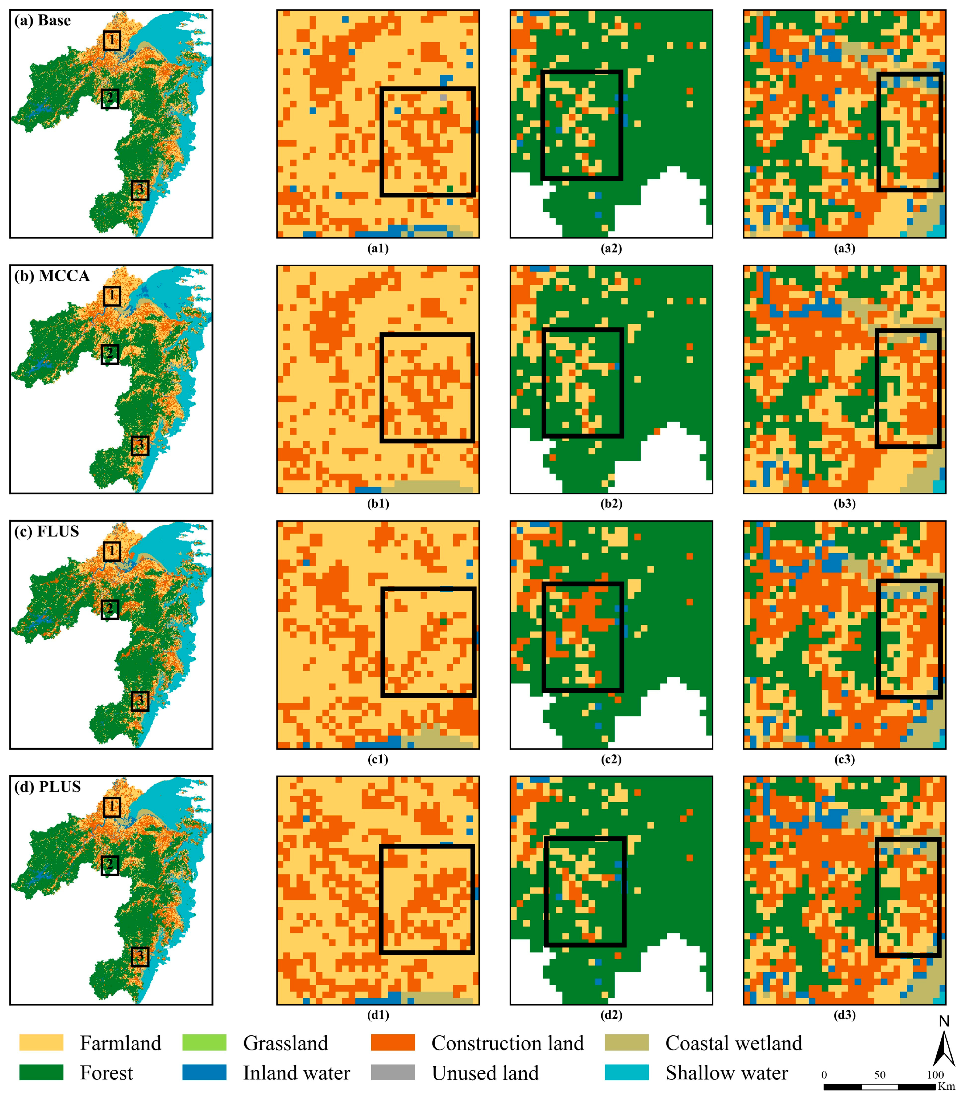
Under consistent driving factors and model training parameters, the FLUS and PLUS models were applied to simulate LULC changes in Zhejiang Province’s coastal zone during 2020. Three representative regions—the northern plains, eastern forested areas, and southeastern coastal plains—were selected from north to south for localized comparative analysis, enabling a comprehensive assessment of model differences.

The 2020 spatial distribution of LULC in Zhejiang Province’s coastal zone simulated by MCCA, FLUS, and PLUS models is compared with actual conditions in Figure 15. This section provides a detailed comparative analysis based on these three representative regions. Results demonstrated that while the spatial distributions of the simulated outputs from all three models shared similarities with actual observations, the accuracy of the MCCA model was demonstrably superior to that of the FLUS and PLUS models. The Kappa coefficient and OA of the MCCA model reached 0.933 and 0.953 respectively, higher than FLUS (0.821 and 0.876) and PLUS (0.854 and 0.898). From a macro perspective, MCCA shows excellent simulation ability and can accurately capture the dynamic changes in LULC patterns.

Figure 14. Simulation accuracies versus aggregated grid size.

Figure 14. Simulation accuracies versus aggregated grid size.

Further local comparison reveals the regional differences in model performance, which are especially obvious under different terrain conditions. In the northern plain of Zhejiang, the MCCA (Figure 15(b1)) simulation results are closer to the actual LULC distribution. The FLUS (Figure 15(c1)) simulation results show that the area of farmland in the northwest is decreasing and the amount of farmland in the southeast region is increasing. The farmland distribution simulated by PLUS (Figure 15(d1)) is relatively scattered. In forested areas, the simulation results of MCCA (Figure 15(b2)) are still the most accurate, while FLUS (Figure 15(c2)) shows a significant expansion of farmland to forested areas, which is a large deviation from the actual situation. PLUS (Figure 15(d2)) did not show a significant deviation as seen in FLUS, but it still tended to overestimate the farmland area. This indicates that there is an error in the FLUS and PLUS models in simulating the expansion of farmland to forested areas. In the southeastern coastal plains, all three models performed well and accurately captured LULC changes.

In summary, the MCCA model can not only accurately reflect the LULC model at the macro level, but also carry out detailed simulation at the local level [44,45].

Figure 15. Comparison of the spatial distribution forecast and the actual situation of three LULC models in 2020. ((a) represents the actual LULC situation; (b–d) represent the MCCA, FLUS and PLUS models respectively; 1–3 correspond to three selected areas, where Box 1 indicates the northern Zhejiang plain region, Box 2 indicates the western forest region, and Box 3 indicates the southeastern coastal plain region).

Figure 15. Comparison of the spatial distribution forecast and the actual situation of three LULC models in 2020. ((a) represents the actual LULC situation; (b–d) represent the MCCA, FLUS and PLUS models respectively; 1–3 correspond to three selected areas, where Box 1 indicates the northern Zhejiang plain region, Box 2 indicates the western forest region, and Box 3 indicates the southeastern coastal plain region).

4.2. Methodological Comparison with Existing Coupling Frameworks

The individual models employed in this framework—SD, MCCA, InVEST, and NSGA-II—are well-established tools in their respective domains. The methodological contribution of this study lies in the synergistic integration that produces advantages unattainable by any single module or conventional coupling configuration.

The MCCA model achieved a simulation accuracy of Kappa = 0.933, substantially outperforming FLUS (0.821) and PLUS (0.854) under identical conditions (Section 4.1). This advantage cannot be attributed to the MCCA algorithm alone. In the SD-FLUS paradigm [27], the one-directional transfer of SD-derived demand to FLUS lacks iterative feedback correction, meaning spatial allocation errors propagate unchecked. Our closed-loop mechanism enforces convergence to within 5% of SD targets, so the accuracy gain reflects the combined effect of causally structured SSP-RCP demand inputs, iterative convergence, and mixed-cell spatial representation. In the PLUS-InVEST paradigm [32], the standard InVEST module assigns carbon density based on a single dominant LULC type per pixel, which would discard the sub-pixel proportional information that the MCCA simulation produces. Our probability-weighted modification (Equation (3)) preserves this information, ensuring the accuracy gained at the simulation stage is not lost at the carbon storage calculation stage. In the NSGA-II-PLUS paradigm [46,47], NSGA-II optimizes aggregate LULC area quantities and PLUS then spatially allocates the result, treating the entire study area uniformly. Our NSGA-II instead operates on pixel-level probability distributions within three spatially differentiated carbon management zones, generating Pareto-optimal solutions where areas experiencing carbon loss, balance, and increase each receive tailored interventions.

The practical significance of this integrated design is demonstrated by the optimization results: the SSP126 scenario achieved simultaneous improvements of 1.16% in carbon storage and 9.05% in economic benefits, confirming that the chain of mutual reinforcement across modules translates into measurable gains. This workflow is intended to provide a replicable methodological reference for LULC-carbon planning in coastal zones and other similarly heterogeneous regions.

4.3. Policy Recommendations

Based on the optimization results of NSGA-II, we propose the strategic framework for coastal zone management in Zhejiang Province as follows:

1.

Enforce strict ecological redlines for high-density carbon sinks.

Optimizing LULC allocation is the basis for improving carbon sink capacity [48]. Previous studies have confirmed that although the high-emission scenario (SSP585) will lead to a serious carbon deficit, the sustainable scenario (SSP126) can successfully reverse this trend [49]. Therefore, conservation work must prioritize forests and coastal wetlands, because the restoration of natural wetlands is crucial to maintaining the function of carbon sequestration [50]. Specifically, the scale of construction land must be strictly limited to 12,000–13,000 km² to prevent encroachment on these ecological spaces.

2.

Implement differentiated spatial zoning strategies.

Management interventions should be adjusted according to the specific characteristics of carbon storage changes [51]:

Carbon Decrease Zones (e.g., the Northern Zhejiang Plain) require aggressive ecological restoration to reverse deforestation and degradation. Carbon Balance Zones should focus on optimizing LULC intensity to maintain stability. Carbon Increase Zones (e.g., western mountainous regions) warrant minimal intervention to preserve existing high-storage structures.

3.

Adopt a phased, dynamic implementation pathway.

Planning adjustment should emphasize phased and dynamic implementation to adapt to the development stage [27]:

Phase I (2020–2040): Prioritize high-storage solutions to quickly restore carbon sinks. Phase II (2040–2070): Pursue synergistic carbon-economic coordination through optimal trade-off strategies. Phase III (2070–2100): Shift management priorities, improve the quality of economic development, and consolidate ecological achievements at the same time.

Finally, considering inter-regional spillover effects [52], we recommend establishing cross-municipal ecological compensation mechanisms. In addition, carbon storage indicators should be included in the local government performance evaluation system to ensure long-term compliance [53]. The dominance of construction land expansion as the primary driver of carbon storage decline observed in this study is not unique to the Zhejiang coastal zone. Similar patterns have been documented in the Guangxi Beibu Gulf coastal economic zone, where continuous construction land growth creates a ‘one increase, many decreases’ trend that severely squeezes ecological land [54], and in the Qingdao coastal zone, where a ‘dual-path coupling’ mechanism was identified linking anthropogenic LULC conversions to changes in carbon-sink and carbon-source land proportions [55]. Our carbon management zoning approach provides a quantitative framework for translating these widely observed trends into spatially differentiated planning interventions. This aligns with the emerging paradigm of carbon-sink-oriented territorial spatial planning, which seeks to embed carbon sequestration targets into LULC allocation decisions [55]. While the specific thresholds proposed here are calibrated to Zhejiang, the underlying principles—controlling construction land expansion rates, enforcing ecological redlines for coastal wetlands and forests, and implementing zone-differentiated management based on carbon storage trends—are transferable to other rapidly urbanizing coastal regions. The framework’s replicability is further supported by its reliance on internationally standardized SSP-RCP scenarios and publicly available datasets.

4.4. Limitations and Future Research

Although the SD-MCCA-NSGA-II integration framework developed in this study has achieved satisfactory results, it still has the following limitations:

4.4.1. Data Limitations

This study relies on several input data assumptions that, while methodologically standard, introduce recognized limitations. First, the static carbon density model deliberately isolates the contribution of LULC transformation to carbon balance by excluding physiological effects (e.g., CO₂ fertilization), but inevitably neglects temporal biological responses such as forest maturation, potentially yielding conservative estimates. Future work could integrate dynamic global vegetation models (DGVMs) with field monitoring data to address this gap. It should be noted that the static carbon density assumption is an inherent design feature of the InVEST carbon storage module, which assumes that all LULC types maintain fixed carbon density values and that changes in carbon storage arise solely from LULC type conversion [56]. This assumption is widely adopted across LULC-carbon coupling studies regardless of the spatial simulation method used [10,29,32,33]. Over shorter simulation horizons (10–30 years), the bias is generally considered acceptable as LULC conversion effects dominate. However, over our 80-year horizon, excluded factors—such as forest maturation, CO₂ fertilization, and climate-driven changes in soil carbon decomposition—may become increasingly significant. This suggests that the model may underestimate carbon storage under the SSP126 scenario (where ecological restoration has the longest time to accumulate biomass) and overestimate it under SSP585 (where extreme climate events may reduce actual carbon density). Nevertheless, because the static assumption applies uniformly across all four scenarios, the relative ranking among scenarios—which is the primary basis for our policy recommendations—is unlikely to be altered. The absolute values should therefore be interpreted as comparative indicators rather than precise predictions. A parallel limitation applies to the economic valuation parameters: although derived from multi-year statistical data (2006–2021) deflated to 2005 constant prices, these values remain static over the projection horizon. Time series forecasting models, such as GM (1,1) or ARIMA, could be employed in future research to enable dynamic economic assessment. Additionally, aggregating daily climate data to annual means—necessary to match the SD model’s annual time step and socioeconomic data resolution—may smooth out extreme seasonal events (e.g., typhoons, storm surges) that acutely impact coastal wetlands. Future studies incorporating sub-annual extreme climate indices could further refine the assessment of episodic climate impacts on coastal ecosystems.

4.4.2. Uncertainty in Scenario Simulation

The SD model reflects the development path under the framework of SSP-RCPs through trend variables, but its accuracy is limited. Parameter relationships calibrated using historical data (2005–2020) may not remain stable over the next 80 years, with this uncertainty increasing as the simulation time scale extends. The model fails to fully consider low-probability, high-impact events, such as extreme weather disasters, technological breakthroughs or sudden policy changes. Furthermore, adaptive responses resulting from shifts in the distribution ranges of forest-forming species under climate change are equally critical but remain insufficiently addressed. There is a pressing need for systematic field observations to monitor the occurrence and migration of forest-forming species, as well as the biogeochemical cycling of matter within these ecosystems, which directly influence long-term carbon storage dynamics. Future research can use Monte Carlo simulation to quantify the uncertainty of parameters and use longer time series data to verify the research results. In addition, the current MCCA model employs random forest regression to predict LULC transition probabilities. Random forest was selected for its demonstrated robustness in handling high-dimensional spatial data, its resistance to overfitting, and its interpretability in identifying key driving factors. Notably, Zhang et al. [57] employed the PLUS model—in which random forest serves as a core algorithmic component—to simulate global LULC at 1 km resolution from 2020 to 2100 under SSP-RCP scenarios, achieving exceptionally high accuracy, further demonstrating the capability of random forest in supporting long-term LULC prediction. Nevertheless, we acknowledge that recent advances in deep learning architectures, such as CNN-LSTM models, have shown promising capabilities in capturing complex non-linear spatiotemporal dynamics [58]. Future research could explore integrating deep learning approaches into the MCCA transition rules to potentially improve long-term prediction accuracy. Moreover, rapid urbanization and the loss of ecological lands under high-emission scenarios may significantly alter local microclimates, particularly through the urban heat island effect, which directly impacts resident thermal comfort, health, and cooling energy demands. These human-centric dimensions are not currently captured in our multi-objective optimization framework. Future iterations could incorporate microclimate simulation and thermal comfort parameters into the optimization objectives, enabling a more holistic assessment that bridges ecological conservation with human well-being in coastal urban environments [59].

4.4.3. Research Directions in Multi-Objective Optimization

This study achieves the dual goal of optimizing carbon storage and economic benefits, but regional sustainable development involves trade-offs in multiple dimensions. Food security requires the protection of farmland, ecological security requires the maintenance of biodiversity, and social equity involves meeting the needs of all stakeholders. In addition, the key parameters of the optimization model (area tolerance ± 5%, adjustment factor $\alpha \in [0.1,0.3]$) lack sensitivity analysis, and the model fails to consider implementation restrictions such as land ownership and land expropriation compensation. Future research may incorporate food security and ecological connectivity into a multi-objective framework and introduce models for the implementation of cost constraints and stakeholder participation to improve the feasibility of the proposed solutions. Furthermore, this study evaluates carbon dynamics primarily from the perspective of land-based carbon storage. However, the substantial expansion of construction land (up to 110.2% under SSP585) inevitably generates significant anthropogenic CO₂ emissions from urban transportation, industrial activities, and infrastructure operations, which are not captured in the current framework. Future studies should integrate micro-level emission inventories with land-based carbon sink assessments to construct a more comprehensive carbon balance for coastal zones [60].

5. Conclusions

This study established the socio-economic path as a decisive factor in coastal carbon dynamics, revealing that the sustainable development scenario (SSP126) can effectively decouple economic growth from carbon loss. By integrating the SD-MCCA framework with NSGA-II optimization, we quantified the trade-offs between protection and development and identified optimal solutions that increased carbon storage by 1.16% while concurrently improving economic benefits by 9.05%.

Distinguishing different spatiotemporal zones—carbon decrease, balance, and increase zones—provides a scientific basis for precise territorial planning. Specifically, our findings emphasize the urgency of protecting coastal wetlands and limiting the expansion of plain cities. Ultimately, this research offers a replicable pathway for coastal regions globally to navigate the complex dual challenges of rapid urbanization and carbon neutrality.

References

1. Hoegh-Guldberg, O.; Jacob, D.; Taylor, M.; Bolaños, T.G.; Bindi, M.; Brown, S.; Camilloni, I.A.; Diedhiou, A.; Djalante, R.; Ebi, K.; et al. The human imperative of stabilizing global climate change at 1.5 °C. Science 2019, 365, eaaw6974. [Google Scholar] [CrossRef] [Scilit]
2. Xi, J. Address to the General Debate of the Seventy-Fifth Session of the United Nations General Assembly. Available online: https://world.huanqiu.com/article/3zzx6TNlCFN (accessed on 14 March 2026).
3. Bongaarts, J. Intergovernmental Panel on Climate Change Special Report on Global Warming of 1.5 °C Switzerland: IPCC, 2018. Popul. Dev. Rev. 2019, 45, 251–252. [Google Scholar] [CrossRef] [Scilit]
4. Crossland, C.J.; Baird, D.; Ducrotoy, J.-P.; Lindeboom, H.; Buddemeier, R.W.; Dennison, W.C.; Maxwell, B.A.; Smith, S.V.; Swaney, D.P. The Coastal Zone—A Domain of Global Interactions. In Coastal Fluxes in the Anthropocene: The Land-Ocean Interactions in the Coastal Zone Project of the International Geosphere-Biosphere Programme; Crossland, C.J., Kremer, H.H., Lindeboom, H.J., Marshall Crossland, J.I., Le Tissier, M.D.A., Eds.; Springer: Berlin/Heidelberg, Germany, 2005; pp. 1–37. [Google Scholar]
5. Ganzenmuller, R.; Obermeier, W.A.; Bultan, S.; Spawn-Lee, S.A.; Zabel, F.; Pongratz, J. Humans have depleted global terrestrial carbon stocks by a quarter. One Earth 2025, 8, 101392. [Google Scholar] [CrossRef] [Scilit]
6. Tang, L.P.; Ke, X.L.; Zhou, T.; Zheng, W.W.; Wang, L.Y. Impacts of cropland expansion on carbon storage: A case study in Hubei, China. J. Environ. Manag. 2020, 265, 110515. [Google Scholar] [CrossRef] [Scilit]
7. Zhang, M.; Huang, X.J.; Chuai, X.W.; Yang, H.; Lai, L.; Tan, J.Z. Impact of land use type conversion on carbon storage in terrestrial ecosystems of China: A spatial-temporal perspective. Sci. Rep. 2015, 5, 10233. [Google Scholar] [CrossRef] [Scilit] [PubMed]
8. Chen, Z.W.; Wei, K.; Hu, L.S.; Yi, C.Q.; Liu, S.Y. Spatiotemporal variation and driving forces of carbon storage in the Fuhe river basin, China. Sci. Rep. 2025, 15, 30224. [Google Scholar] [CrossRef] [Scilit]
9. Jin, T.L.; Zhang, P.X.; Zhou, N.; Li, S. Unveiling the spatiotemporal heterogeneity and driving mechanisms of carbon storage changes in response to land use/land cover changes under different future scenarios: Insights from the GMOP-SEM model. J. Clean. Prod. 2025, 487, 144622. [Google Scholar] [CrossRef] [Scilit]
10. Wu, Q.; Wang, L.; Wang, T.Y.; Ruan, Z.Y.; Du, P. Spatial-temporal evolution analysis of multi-scenario land use and carbon storage based on PLUS-InVEST model: A case study in Dalian, China. Ecol. Indic. 2024, 166, 112448. [Google Scholar] [CrossRef] [Scilit]
11. Wu, W.H.; Xu, L.Y.; Zheng, H.Z.; Zhang, X.R. How much carbon storage will the ecological space leave in a rapid urbanization area? Scenario analysis from Beijing-Tianjin-Hebei Urban Agglomeration. Resour. Conserv. Recycl. 2023, 189, 106774. [Google Scholar] [CrossRef] [Scilit]
12. Xu, C.L.; Zhang, Q.B.; Yu, Q.; Wang, J.P.; Wang, F.; Qiu, S.; Ai, M.S.; Zhao, J.K. Effects of land use/cover change on carbon storage between 2000 and 2040 in the Yellow River Basin, China. Ecol. Indic. 2023, 151, 110345. [Google Scholar] [CrossRef] [Scilit]
13. Zhang, D.; Huang, Q.X.; He, C.Y.; Yin, D.; Liu, Z.W. Planning urban landscape to maintain key ecosystem services in a rapidly urbanizing area: A scenario analysis in the Beijing-Tianjin-Hebei urban agglomeration, China. Ecol. Indic. 2019, 96, 559–571. [Google Scholar] [CrossRef] [Scilit]
14. Zhang, Z.; Jiang, W.G.; Peng, K.F.; Wu, Z.F.; Ling, Z.Y.; Li, Z. Assessment of the impact of wetland changes on carbon storage in coastal urban agglomerations from 1990 to 2035 in support of SDG15.1. Sci. Total Environ. 2023, 877, 162824. [Google Scholar] [CrossRef] [Scilit]
15. Riahi, K.; van Vuuren, D.P.; Kriegler, E.; Edmonds, J.; O’Neill, B.C.; Fujimori, S.; Bauer, N.; Calvin, K.; Dellink, R.; Fricko, O.; et al. The Shared Socioeconomic Pathways and their energy, land use, and greenhouse gas emissions implications: An overview. Glob. Environ. Change 2017, 42, 153–168. [Google Scholar] [CrossRef] [Scilit]
16. van Vuuren, D.P.; Edmonds, J.; Kainuma, M.; Riahi, K.; Thomson, A.; Hibbard, K.; Hurtt, G.C.; Kram, T.; Krey, V.; Lamarque, J.F.; et al. The representative concentration pathways: An overview. Clim. Change 2011, 109, 5–31. [Google Scholar] [CrossRef] [Scilit]
17. Zhang, D.; Huang, Q.X.; He, C.Y.; Wu, J.G. Impacts of urban expansion on ecosystem services in the Beijing-Tianjin-Hebei urban agglomeration, China: A scenario analysis based on the Shared Socioeconomic Pathways. Resour. Conserv. Recycl. 2017, 125, 115–130. [Google Scholar] [CrossRef] [Scilit]
18. Zeng, L.; Liu, X.P.; Li, W.H.; Ou, J.P.; Cai, Y.L.; Chen, G.Z.; Li, M.C.; Li, G.D.; Zhang, H.H.; Xu, X.C. Global simulation of fine resolution land use/cover change and estimation of aboveground biomass carbon under the shared socioeconomic pathways. J. Environ. Manag. 2022, 312, 114943. [Google Scholar] [CrossRef] [Scilit] [PubMed]
19. Liang, X.; Guan, Q.F.; Clarke, K.C.; Chen, G.Z.; Guo, S.; Yao, Y. Mixed-cell cellular automata: A new approach for simulating the spatio-temporal dynamics of mixed land use structures. Landsc. Urban Plan. 2021, 205, 103960. [Google Scholar] [CrossRef] [Scilit]
20. Zhang, J.T.; Yang, K.; Wu, J.D.; Duan, Y.; Ma, Y.N.; Ren, J.Z.; Yang, Z.N. Scenario simulation of carbon balance in carbon peak pilot cities under the background of the “dual carbon” goals. Sustain. Cities Soc. 2024, 116, 105910. [Google Scholar] [CrossRef] [Scilit]
21. Chen, G.Z.; Li, X.; Liu, X.P.; Chen, Y.M.; Liang, X.; Leng, J.Y.; Xu, X.C.; Liao, W.L.; Qiu, Y.A.; Wu, Q.L.; et al. Global projections of future urban land expansion under shared socioeconomic pathways. Nat. Commun. 2020, 11, 537. [Google Scholar] [CrossRef] [Scilit]
22. Jiang, T.; Zhao, J.; Cao, L.-G.; Wang, Y.-J.; Su, B.-D.; Jing, C.; Wang, R.; Gao, C. Projection of national and provincial economy under the shared socioeconomic pathways in China. Clim. Change Res. 2018, 14, 50–58. (In Chinese) [Google Scholar] [CrossRef]
23. Zuo, J.; Zhang, L.; Xiao, J.; Chen, B.; Zhang, B.; Hu, Y.; Al Mamun, M.M.A.; Wang, Y.; Li, K. GCL_FCS30: A global coastline dataset with 30-m resolution and a fine classification system from 2010 to 2020. Sci. Data 2025, 12, 129. [Google Scholar] [CrossRef] [Scilit]
24. Yuan, H.H.; Ning, L.K.; Zhou, J.W.; Shi, W.; Huang, J.B.; Luo, Y. HiCPC: A new 10-km CMIP6 downscaled daily climate projections over China. Sci. Data 2024, 11, 1167. [Google Scholar] [CrossRef] [Scilit] [PubMed]
25. Zhang, X.; Zhao, T.T.; Xu, H.; Liu, W.D.; Wang, J.Q.; Chen, X.D.; Liu, L.Y. GLC_FCS30D: The first global 30 m land-cover dynamics monitoring product with a fine classification system for the period from 1985 to 2022 generated using dense-time-series Landsat imagery and the continuous change-detection method. Earth Syst. Sci. Data 2024, 16, 1353–1381. [Google Scholar] [CrossRef] [Scilit]
26. Song, B.-y.; Hou, X.-y.; Wang, X.-l.; Liu, Y.-b. Multi-scenario simulation of land use change in coastal zones —A case study of Shandong coastal zone. Mar. Sci. 2020, 46, 22–33. (In Chinese) [Google Scholar] [CrossRef]
27. Hou, X.Y.; Song, B.Y.; Zhang, X.Y.; Wang, X.L.; Li, D. Multi-scenario Simulation and Spatial-temporal Analysis of LUCC in China’s Coastal Zone Based on Coupled SD-FLUS Model. Chin. Geogr. Sci. 2024, 34, 579–598. [Google Scholar] [CrossRef] [Scilit]
28. Huang, Z.H.; Li, X.J.; Du, H.Q.; Mao, F.J.; Han, N.; Fan, W.L.; Xu, Y.X.; Luo, X. Simulating Future LUCC by Coupling Climate Change and Human Effects Based on Multi-Phase Remote Sensing Data. Remote Sens. 2022, 14, 1698. [Google Scholar] [CrossRef] [Scilit]
29. Wang, Z.Y.; Li, X.; Mao, Y.T.; Li, L.; Wang, X.R.; Lin, Q. Dynamic simulation of land use change and assessment of carbon storage based on climate change scenarios at the city level: A case study of Bortala, China. Ecol. Indic. 2022, 134, 108499. [Google Scholar] [CrossRef] [Scilit]
30. Carpenter, S.R.; Bennett, E.M.; Peterson, G.D. Scenarios for ecosystem services: An overview. Ecol. Soc. 2006, 11, 29. [Google Scholar] [CrossRef] [Scilit]
31. Alcamo, J.; Henrichs, T. Chapter Two Towards Guidelines for Environmental Scenario Analysis. Dev. Integr. Environ. Assess. 2008, 2, 13–35. [Google Scholar] [CrossRef] [Scilit]
32. Li, H.J.; Zhang, K.; Liu, Y.Q.; Qin, Y.; Wang, W.P.; Wang, M.Y.; Liu, Y.N.; Li, Y.Q. Spatiotemporal evolution of land use and carbon storage in China: Multi-Scenario simulation and driving factor analysis based on the PLUS-InVEST model and SHAP. Environ. Res. 2025, 279, 121860. [Google Scholar] [CrossRef] [Scilit] [PubMed]
33. Jiang, W.G.; Deng, Y.; Tang, Z.H.; Lei, X.; Chen, Z. Modelling the potential impacts of urban ecosystem changes on carbon storage under different scenarios by linking the CLUE-S and the InVEST models. Ecol. Model. 2017, 345, 30–40. [Google Scholar] [CrossRef] [Scilit]
34. Lai, J.L.; Qi, S.; Chen, J.D.; Guo, J.C.; Wu, H.; Chen, Y.Z. Exploring the spatiotemporal variation of carbon storage on Hainan Island and its driving factors: Insights from InVEST, FLUS models, and machine learning. Ecol. Indic. 2025, 172, 113236. [Google Scholar] [CrossRef] [Scilit]
35. Alam, S.A.; Starr, M.; Clark, B.J.F. Tree biomass and soil organic carbon densities across the Sudanese woodland savannah: A regional carbon sequestration study. J. Arid Environ. 2013, 89, 67–76. [Google Scholar] [CrossRef] [Scilit]
36. Li, H.Y.; Hu, Y.T.; Li, H.; Ren, J.J.; Shao, R.J.; Liu, Z.C. Assessing the Impact of Spatiotemporal Evolution of Urbanization on Carbon Storage in the Mega-Urban Agglomeration Area: Case Study of Yangtze River Delta Urban Agglomeration, China. Sustainability 2023, 15, 14548. [Google Scholar] [CrossRef] [Scilit]
37. Ma, Z.Y.; Duan, X.J.; Wang, L.; Wang, Y.Z.; Kang, J.Y.; Yun, R.X. A Scenario Simulation Study on the Impact of Urban Expansion on Terrestrial Carbon Storage in the Yangtze River Delta, China. Land 2023, 12, 297. [Google Scholar] [CrossRef] [Scilit]
38. Wang, Y.R.; Jiang, X.Q.; Gao, S.; Jiang, Q.; Du, H.Q.; Han, N. Multi-scenario carbon storage analysis based on PLUS model and InVEST model: A case study of Zhejiang province, China. Earth Sci. Inform. 2025, 18, 192. [Google Scholar] [CrossRef] [Scilit]
39. Deb, K.; Pratap, A.; Agarwal, S.; Meyarivan, T. A fast and elitist multiobjective genetic algorithm: NSGA-II. IEEE Trans. Evol. Comput. 2002, 6, 182–197. [Google Scholar] [CrossRef] [Scilit]
40. Wang, Y.; Shen, J.; Yan, W.; Chen, C. Backcasting approach with multi-scenario simulation for assessing effects of land use policy using GeoSOS-FLUS software. MethodsX 2019, 6, 1384–1397. [Google Scholar] [CrossRef] [Scilit]
41. Macreadie, P.I.; Costa, M.D.P.; Atwood, T.B.; Friess, D.A.; Kelleway, J.J.; Kennedy, H.; Lovelock, C.E.; Serrano, O.; Duarte, C.M. Blue carbon as a natural climate solution. Nat. Rev. Earth Environ. 2021, 2, 826–839. [Google Scholar] [CrossRef] [Scilit]
42. Aryal, D.R.; Enrique Morales-Ruiz, D.; Lopez-Cruz, S.; Noe Tondopo-Marroquin, C.; Lara-Nucamendi, A.; Antonio Jimenez-Trujillo, J.; Perez-Sanchez, E.; Edduardo Betanzos-Simon, J.; Casasola-Coto, F.; Martinez-Salinas, A.; et al. Silvopastoral systems and remnant forests enhance carbon storage in livestock-dominated landscapes in Mexico. Sci. Rep. 2022, 12, 16769. [Google Scholar] [CrossRef] [Scilit]
43. Hoosbeek, M.R.; Remme, R.P.; Rusch, G.M. Trees enhance soil carbon sequestration and nutrient cycling in a silvopastoral system in south-western Nicaragua. Agrofor. Syst. 2018, 92, 263–273. [Google Scholar] [CrossRef] [Scilit]
44. Jiang, X.; Duan, H.; Liao, J.; Song, X.; Xue, X. Multi-model-based Simulation of Different Landuse Scenarios in Gan Lin Gao Area in Middle Reaches of Heihe River. Trans. Chin. Soc. Agric. Mach. 2022, 50, 178–188. (In Chinese) [Google Scholar] [CrossRef]
45. Zhang, P.; Liu, L.; Yang, L.W.; Zhao, J.; Li, Y.Y.; Qi, Y.T.; Ma, X.N.; Cao, L. Exploring the response of ecosystem service value to land use changes under multiple scenarios coupling a mixed-cell cellular automata model and system dynamics model in Xi’an, China. Ecol. Indic. 2023, 147, 110009. [Google Scholar] [CrossRef] [Scilit]
46. Luan, C.; Liu, R.; Zhang, Q.; Sun, J.; Liu, J. Multi-objective land use optimization based on integrated NSGA-II-PLUS model: Comprehensive consideration of economic development and ecosystem services value enhancement. J. Clean. Prod. 2024, 434, 140306. [Google Scholar] [CrossRef] [Scilit]
47. Gu, H.; Liu, S.; Huan, C.; Cheng, M.; Dong, X.; Sun, H. Multi-Objective Land Use Optimization Based on NSGA-II and PLUS Models: Balancing Economic Development and Carbon Neutrality Goals. Land 2025, 14, 1585. [Google Scholar] [CrossRef] [Scilit]
48. Ye, C.Y.; Ming, T. Land use carbon emissions estimation and carbon emissions control strategy effect scenario simulation in Zhejiang province. Heliyon 2023, 9, e20783. [Google Scholar] [CrossRef] [Scilit]
49. Gao, F.J.; Xin, X.H.; Song, J.X.; Li, X.W.; Zhang, L.; Zhang, Y.; Liu, J.F. Simulation of LUCC Dynamics and Estimation of Carbon Stock under Different SSP-RCP Scenarios in Heilongjiang Province. Land 2023, 12, 1665. [Google Scholar] [CrossRef] [Scilit]
50. Zhou, Y.; Han, Z. Spatial and Temporal Variation of Carbon Storage from Coastal Zone Planning and Management Perspective. Remote Sens. Inf. 2023, 38, 11–17. (In Chinese) [Google Scholar] [CrossRef]
51. Xue, H.; Shi, Z.Q.; Huo, J.G.; Zhu, W.B.; Wang, Z.Y. Spatial difference of carbon budget and carbon balance zoning based on land use change: A case study of Henan Province, China. Environ. Sci. Pollut. Res. 2023, 30, 109145–109161. [Google Scholar] [CrossRef] [Scilit]
52. Bai, Y.; Deng, X.; Jiang, S.; Zhang, Q.; Wang, Z. Exploring the relationship between urbanization and urban eco-efficiency: Evidence from prefecture-level cities in China. J. Clean. Prod. 2018, 195, 1487–1496. [Google Scholar] [CrossRef] [Scilit]
53. Han, F.; Huang, M. Land Misallocation and Carbon Emissions: Evidence from China. Land 2022, 11, 1189. [Google Scholar] [CrossRef] [Scilit]
54. Jiang, H.; Cui, Z.; Fan, T.; Yin, H. Impacts of land use change on carbon storage in the Guangxi Beibu Gulf Economic Zone based on the PLUS-InVEST model. Sci. Rep. 2025, 15, 6468. [Google Scholar] [CrossRef] [Scilit]
55. Xu, C.; Wang, C.; Liu, D.; Zhang, Z.; Li, Y.; Li, Z. Evolution of carbon sink patterns and spatial planning suitability in the Qingdao Coastal Zone based on the coupled InVEST–PLUS model. Front. Mar. Sci. 2026, 13, 1749473. [Google Scholar] [CrossRef] [Scilit]
56. Alliance, N.C. InVEST, 3.18.0; Stanford University: Stanford, CA, USA, 2026.
57. Zhang, T.; Cheng, C.; Wu, X. Mapping the spatial heterogeneity of global land use and land cover from 2020 to 2100 at a 1 km resolution. Sci. Data 2023, 10, 748. [Google Scholar] [CrossRef] [Scilit] [PubMed]
58. Wang, Z.; Mae, M.; Yamane, T.; Ajisaka, M.; Nakata, T.; Matsuhashi, R. Novel Custom Loss Functions and Metrics for Reinforced Forecasting of High and Low Day-Ahead Electricity Prices Using Convolutional Neural Network-Long Short-Term Memory (CNN-LSTM) and Ensemble Learning. Energies 2024, 17, 4885. [Google Scholar] [CrossRef] [Scilit]
59. Wang, Z.; Matsuhashi, R.; Onodera, H. Intrusive and non-intrusive early warning systems for thermal discomfort by analysis of body surface temperature. Appl. Energy 2023, 329, 120283. [Google Scholar] [CrossRef] [Scilit]
60. Wang, Z.; Mae, M.; Nishimura, S.; Matsuhashi, R. Vehicular Fuel Consumption and CO2 Emission Estimation Model Integrating Novel Driving Behavior Data Using Machine Learning. Energies 2024, 17, 1410. [Google Scholar] [CrossRef] [Scilit]
Figure 1. Study Area Location Map.
Land 15 00648 g001
Figure 3. Research Framework Diagram.
Land 15 00648 g003
Figure 4. Flowchart of the NSGA-II optimization process. The dashed arrow indicates the generational iteration loop.
Land 15 00648 g004
Figure 5. Relative Entropy Distribution of 2020 Simulation Results.
Land 15 00648 g005
Figure 7. Simulation Results of LULC Under Different Scenarios in 2100 ((a) Spatial distribution of LULC and average probability and maximum probability pie charts under SSP126 scenario; (b) Spatial distribution of LULC under the SSP245 scenario, along with average probability and maximum probability pie charts; (c) Spatial distribution of LULC under the SSP370 scenario, along with average probability and maximum probability pie charts; and (d) Spatial distribution of LULC under the SSP585 scenario, along with average probability and maximum probability pie charts). For visual clarity, land-use categories with probabilities lower than 0.15 are not displayed in the pie charts.
Land 15 00648 g007
Figure 8. Simulated Carbon Storage Results under Different Scenarios in 2100 ((a) Carbon storage estimates under the SSP126 scenario, (b) carbon storage estimates under the SSP245 scenario, (c) carbon storage estimates under the SSP370 scenario, and (d) carbon storage estimates under the SSP585 scenario. The blue boxes indicate distinct clusters of reduced carbon storage.)
Land 15 00648 g008
Figure 9. Carbon Storage Zoning Results Under Different Scenarios ((a) Carbon storage zoning results under the SSP126 scenario, (b) Carbon storage zoning results under the SSP245 scenario, (c) Carbon storage zoning results under the SSP370 scenario, and (d) Carbon storage zoning results under the SSP585 scenario).
Land 15 00648 g009
Figure 10. Contributions of Different LULC Types to Carbon Storage ((a) Contributions under SSP126 Scenario, (b) Contributions under SSP245 Scenario, (c) Contributions under SSP370 Scenario, and (d) Contributions under SSP585 Scenario).
Land 15 00648 g010