Abstract
An important motivation for the implementation of the Water Framework Directive is the creation of non-market environmental benefits, such as improved ecological quality, or greater opportunities for open-access river recreation via microbial pollution remediation. Pollution sources impacting on ecological or recreational water quality may be uncorrelated, but non-market benefits arising from riverine improvements are typically conflated within benefit valuation studies. Using stated preference choice experiments embedded within a survey that also collected respondents’ socio-economic characteristics, we aimed to disaggregate these sources of value for different river users, thereby allowing decision makers to understand the consequences of adopting alternative investment strategies. Our results suggested that anglers derived greater value from improvements to the ecological quality of river water, in contrast to swimmers and rowers, for whom greater value is gained from improvements to recreational quality. More generally, we found three distinct groups of respondents: a majority preferring ecological over recreational improvements, a substantial minority holding opposing preference orderings, and a yet smaller proportion expressing relatively low values for either form of river quality enhancement. As such, this research demonstrates that the non-market benefits that may accrue from different types of water quality improvements are nuanced in terms of their potential beneficiaries and, by inference, their overall value and policy implications.
1. Introduction
The Water Framework Directive (WFD) requires substantial improvements to the quality of Europe’s waters so that the ‘good ecological status’ of surface waters is achieved [1]. One important motivation for the implementation of the WFD appears to be the creation of non-market social benefits such as improved provision of, and opportunities for, open-access recreation (Articles 4, 9 and 11 of the WFD).
Previous research has shown that it is technically infeasible and prohibitively expensive for all UK rivers to be brought to ‘good ecological status’ within the near future [2]. The WFD allows derogations from ‘good ecological status’ where remediation projects may be technically infeasible, or where remediation costs may be disproportionate to the benefits created (Article 4, par. 4, 5, 7). The financial costs of pollution remediation must be offset against the benefits of that remediation. Some benefits may be measured on the market, and are commonly accounted for in water management plans [3]. Official UK guidelines state that non-market costs and benefits must not be ignored, but must be ‘quantified where possible and meaningful’ [4]. Therefore the role of economics is crucial in assessing the non-market benefits of measures that could be implemented to achieve WFD targets, as these benefit values may represent significant components of water quality improvements [5].
Among economic valuation techniques, stated preference methods have been extensively used for valuing the non-market benefits arising from environmental improvements, with choice experiments (CE) being used since the late 1990s for water quality studies. This trend has continued over the last 10 years, with the method being used to assess a diverse range of water quality issues, including assessments of wetland conservation projects [6], multi-country assessments of benefit transfer in water conservation projects [7], and adaptations to river use [8]. Well-designed stated preference CEs produce consistent, valid and reliable estimates that may be used to support decision making [9].
Valuation studies typically assess WFD benefits in ways that conflate the value of ecological improvements with the value of microbial pollution reduction, therefore assessing water quality as a single attribute of preference [10,11]. However, the ecological and microbial attributes of water are not identical. They are affected differently by different pollutants. Moreover, different benefits accrue from remediation measures designed to reduce either type of pollution. Ecological quality is relevant for diverse healthy aquatic ecosystems, and is principally determined by diffuse nutrient pollution (e.g., nitrates and phosphates) from agriculture. Microbiological quality is relevant for recreation (i.e., reduction of the risk of ill-health via microbial pollution reduction leads to improved opportunities for safer recreation [12]) and is largely determined by faecal pollution, typically from livestock and/or wastewater treatment works [13]. Doherty et al. [14] observe that ‘a consequence of focusing on just the ecological status of the water bodies being analysed is that the marginal value of a specific characteristic of a waterbody (e.g., the marginal value of a change in the recreational or aesthetic attribute) cannot be estimated’.
In the UK, the most recent CE water quality studies include Hanley et al. [15], Glenk et al. [11], Metcalfe et al. [16] and Doherty et al. [14]. Hanley et al., provide willingness to pay (WTP) measures for improvements from fair to good for ecological quality, aesthetic, and bankside condition attributes of the rivers Wear (Durham) and Clyde (Central Scotland). Glenk et al., and Metcalfe et al., describe the state of water bodies (rivers and lochs in the former and all water bodies in the latter) and assess respondents’ preferences for the potential future status of those water bodies. Doherty et al., disentangle water quality characteristics into aquatic ecosystem health, water clarity and odour attributes. None of these studies sought to separate the microbiological/recreational component of water quality from the ecological attribute.
The main aim of this research was to further the knowledge on non-market valuation of river water by disaggregating the values people derived from ecological and microbial aspects of river water quality. Given the link between microbial quality and recreational river use, we investigated how the values for these distinct attributes of river water quality differed over people who (i) engaged with the river in different ways (rowers, swimmers, anglers) and (ii) who lived at different distances from the river. This investigation was undertaken using a stated preference, Discrete Choice Experiment (DCE), with discrete attributes for ecological and recreational water characteristics.
Our results indicated significant heterogeneity in water quality preferences: a majority of respondents preferred ecological improvements, a substantial minority preferred recreational improvements, and a small proportion held relatively low values for either form of river quality enhancement. Anglers prioritised ecological quality, while swimmers and rowers favour improved recreational opportunities. A clear distance decay in respondents’ WTP values away from the site of proposed investment was revealed. As such, this research demonstrates that the non-market benefits that may accrue from different types of water quality improvements are nuanced in terms of their environmental impacts, their potential beneficiaries and, by inference, their overall value and policy implications. This information allows decision makers to better understand the consequences of adopting alternative investment strategies that favour either ecological or recreational improvements, or a mix of benefits, as these trade-offs were previously poorly understood [17].
2. Materials and Methods
2.1. Case Study Area and Catchment
The survey was conducted in Norfolk, UK. The River Yare was selected as a case study area to study ecological and recreational values. The Yare catchment is predominantly rural, supporting agriculture and horticulture, but is prone to diffuse agricultural pollution from nutrients (primarily phosphates). The catchment has been identified as a High Water Quality Priority Area for Catchment Sensitive Farming advice and Countryside Stewardship, as it fails to meet WFD targets [18]. The catchment also has difficulties meeting WFD targets due to point source pollution discharges (e.g., inadequately treated wastewater) from the water industry [19]. The population of the Yare catchment is concentrated within the city of Norwich, a city of 210,000 inhabitants. Wastewater from the Norwich area is processed at a treatment facility located near the village of Postwick, two miles to the south-east of the city. Figure 1 shows the survey area, the locations of respondents’ homes and the 20 km survey stretch of the River Yare.
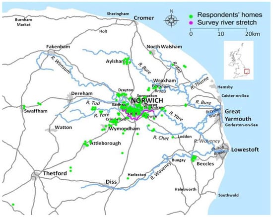
Figure 1.
The survey area, survey river stretch and spatial distribution of respondents.
2.2. Survey Instruments and Choice Experiment Design
Water quality attributes span a continuum ranging from those that can be easily perceived (e.g., algal growth), to characteristics imperceptible to human senses (e.g., concentrations of microbial organisms). To aid experimental accuracy, researchers have sought to produce objective water quality indices to convey information to respondents, using combinations of scientifically quantified parameters [20]. These indices, displayed graphically to respondents as water quality ladders, are increasingly standardised and used to obtain accurate estimates of water quality benefits within economic valuation studies [21,22].
Unfortunately, a common characteristic of water quality ladders is that they conflate ecological and microbiological quality attributes [21]. We disaggregated the water quality ladder developed by Hime et al. [22] into ecological and recreational components. To sufficiently address our research question, yet minimise the cognitive load on respondents, we used three simple attributes to describe water quality across a range of future water quality scenarios at the survey river stretch (Figure 2). Ecological quality had four levels ranging from ‘blue’ (the highest) to ‘red’ (the lowest). These levels were based on United Kingdom Technical Advisory Group (UKTAG) guidance [23]. UKTAG is a partnership of the UK environment and conservation agencies that was created to provide coordinated advice on the scientific and technical aspects of implementing the WFD. Microbiologically polluted water has been shown to have a dose-response relationship with the risk of ill-health (i.e., the rate of infection among recreational users increases steadily with increasing concentrations of harmful microorganisms and, for a constant concentration of microorganisms, the rate of infection is higher for those recreational users who have higher exposure) [12]. Our recreational quality ladder had three levels; ‘high’, ‘medium’ and ‘low’, which corresponded to the acceptable risk of ill-health for different activities, e.g., a river of ‘medium’ recreational quality may be unsuitable for full immersion activities such as swimming (due to high concentrations of harmful bacteria), but may still be suitable for activities such as rowing (rowers, who are usually only splashed by contaminated water, have lower exposure and a lower risk of ill-health). The price had eight levels ranging from £0 to £100. The payment vehicle was presented as a hypothetical increase to the respondents’ annual domestic water bill. The payment vehicle corresponded with those used in previous studies on water quality improvements in public areas [11,24]. We believed that this approach would be most appropriate as, in the UK, domestic water bills also include a sum towards improving wastewater services that, in turn, leads to improved river water quality.
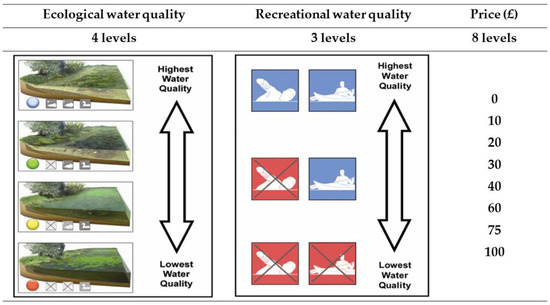
Figure 2.
Choice experiment attributes and levels.
A common characteristic of CEs is the inclusion of a constant level of environmental quality (the ‘status quo’) within the choice task and, within such studies, respondents could prefer the status quo to any proposed change. The status (health) of the water environment of the river Yare, and its tributary rivers, was assessed by the Environment Agency in 2013 as being generally ‘moderate’ [19]. That assessment broadly corresponds to the ‘green’ ecological and ‘medium’ recreational water quality attributes used in our study. Defining the status quo in water quality studies is problematic, as attributes vary according to river morphology, season, geographical location, etc., and encapsulating these variable components into a single fixed state may be overly restrictive. Furthermore, respondents are often heterogeneously and imperfectly informed, and their perceptions of the ‘status quo’ may bear little or no resemblance to reality [25,26]. This divergence can reduce the accuracy of welfare estimates: Poor et al. [27] demonstrate the impact of objective vs. perceived measures in valuing the water clarity of lakes in Maine. This study circumvented these issues in two ways. We collected the perceptions of water quality directly from respondents and incorporated those perceptions into welfare benefit valuations. We also used a forced choice design, in which there was no ’status quo’ opt out option included in each set. The absence of a ’current‘ option reflected the reality of water management in the context of the study: the status quo was not an option due to the implementation of WFD-induced water quality improvement programmes. Forced choice designs have been used in other water DCE studies where the status quo is no longer an option [28,29]. Welfare analysis is still possible as long as the current levels of the attributes are included in the experimental design. Questions to capture other variation in WTP (e.g., distance, respondents’ socio-economic characteristics and use patterns) were included elsewhere within the survey.
The combination of attributes and levels used on choice cards was derived following the D-efficient design strategy. This strategy ensured that the choice cards’ combinations were balanced and maximized the parameter precision of a conditional logit (CL) model. D error is the determinant of the variance covariance matrix of the conditional model and is directly linked to parameters precision. The D error was 0.306965. An alternative efficiency measure is the A error, which considers the trace of the variance-covariance method. The A error in this design was 1.631721. The parameters precision is higher when these efficiency measures are closer to 0. The resulting design yielded a higher efficiency level than those typically observed in the wider literature. Further details on D-efficient design can be found in Ferrini and Scarpa, 2007 [30] and in the Ngene v.1.1 manual [31]. In total, 48 combinations were produced, which were arranged into four blocks of 12 choices, with each block presented to 50 respondents, for a total of 200 respondents.
A recruitment strategy was devised that differentiated between river visitors (who deliberately visited rivers within the previous year) and non-visitors and, of those respondents who identified as visitors, captured different recreation types.
To follow best practice [9], care was taken to reflectively develop all aspects of the survey instruments and design the survey’s implementation procedures to best maximize the validity and reliability of the resulting utility estimates. We considered these issues to be crucial to obtain unbiased estimates which could add to the growing literature on non-market benefit valuation. Within the survey instrument design, our goal was to use simple language and graphics to portray complex information relating to ecological and microbial pollution, and provide respondents with accurate, unbiased information on different water options, choice outcomes and associated costs (the survey questionnaire and showcards are given as Supplementary Materials to this paper). Terms that respondents could easily comprehend were used throughout, as the majority of respondents were expected to have little or no prior knowledge of river water quality issues. The survey instruments and experimental design were pre-tested. Within the main survey data collection, we were mindful to reduce information bias: each respondent was provided with almost exactly the same information from which to aid their choice decisions, and that information was carefully considered to prevent excess information disclosure which could lead to inflated utility estimates [32]. A single interviewer conducted the interviews, and as far as possible, did not deviate in appearance or demeanor, to minimise interviewer variability and bias [33].
2.3. Modelling Strategies
2.3.1. Conditional Logit Modelling
The CL model is frequently used in choice modelling studies to estimate the impact of water characteristics (also called attributes) and respondents’ socio-economic characteristics on the utility of different alternatives [34]. We assumed that the respondent compared the levels of attributes for each water scenario alternative and chose the option that maximized their utility. Following Random Utility Maximization theory [35], the utility of each water scenario (j) can be formalized as:
where xijt is a K-vector of water characteristics of alternative j facing person i on occasion t, βi is a vector of parameters to be estimated and represents person i specific utility weights on water attributes, and εijt is the error term. In order to estimate the β parameters, the researcher could follow different modelling strategies dictated by the specification of the error term εijt.
Uijt = Vijt + eijt = βxijt + εijt, i = 1,…., N (respondents); j = 1,…, J (alternatives); t = 1,…, T (repetitions)
Assuming that the error component is identical and independently distributed as Extreme Value Type I [35], and the chosen option [yit] is j among the J alternatives, the CL model can be formalized as:
The CL is the most common standard specification model for choice data and can be estimated with maximum likelihood techniques. Preference heterogeneity can be incorporated into the model by interacting socio-economic variables with choice attributes.
Unfortunately, the CL model has several drawbacks [36]. Repeated observations by the same respondent cannot be accommodated by the model, heterogeneity in preference cannot be properly addressed, and correlation among alternatives cannot be estimated. McFadden and Train [37] provide the Lagrange Multiplier test that uses artificial variables to verify heterogeneity in preferences and verifies whether the distributional assumption on the error components is supported by data. Dropping the t-index for simplicity, the artificial variables can be obtained as:
where Pij is the CL choice probability. The CL model in Equation (2) is re-estimated including the artificial variables, and the null hypothesis of no random coefficients on attributes x is rejected if the coefficients for the artificial variables are significantly different from zero. When the test fails to reject the null, the implication is that the CL assumption on the error term is inappropriate, and other assumptions must be tested. An alternative model specification is latent class (LC), which overcomes CL limitations in addressing preference heterogeneity [38] and repeated choices [39].
2.3.2. Latent Class Analysis
The LC model posits that preferences can be explained by observable and latent factors [40]. The model structure is extended to accommodate unobservable heterogeneity explained by socio-economic characteristics or attitudinal/psychological information [41]. From a policy perspective, LC analysis enables environmental managers to respond more appropriately to the preferences of those subgroups [42]. There has been a growing use of LC to assess environmental preferences, e.g., in recreational angling [43], wilderness recreation [44], and reservoir recreation [45].
The LC model clusters respondents within relatively homogenous classes, and for each class, the parameter of water characteristics (β) is estimated. Each respondent can be probabilistically assigned to any class, given personal characteristics, and the final result is a set of preference parameters for each group. Thus the LC model captures preference heterogeneity through the error component specification strategy and solves many of the limitations of CL model specification.
Formally, a LC model uses a probabilistic class allocation model, and a CL model for the alternative choices. Each respondent i belongs to class s (of S classes) with probability πis, with and. The probability that respondent i belongs to class s is:
where δs is a class specific constant, zi is a vector of individual socio-economic characteristics, and γs is a vector of parameters to be estimated, capturing the impact of respondents’ characteristics on preferences.
Conditional on the probability of being in class s the probability of choosing option j among the J alternatives is equivalent to Equation (2). The unconditional probability of choosing option j for respondent i for choice situation t = 1 is the product of Equations (2) and (4):
In common with the CL specification, maximum likelihood procedures can be used to estimate the LC model. Respondents’ individual class membership probabilities were calculated using the method described in Morey and Thacher [46], which enables each respondent to be allocated to their most likely class using that individual’s conditional class-membership probabilities. Post-estimation results were then defined using class members’ socio-economic characteristics.
Following welfare theory [47], both models can provide marginal welfare values by the ratio of marginal utility of each attribute (k) and price (p):
The WTP ratio can be derived when we can observe a marginal change from the initial state of water and a future change. The choice setting deliberately avoided defining the current water quality level (status quo) and the survey collected information on perceived water quality. We estimated WTP in two ways: we used ‘low’ ecological or recreational quality as objective initial water quality states, or, as in Hynes et al. [48], we use respondents’ perceptions of water quality. We considered, at the individual level, the perceived water quality and where that respondent’s perception was lower than the improvement, WTP was set to zero (e.g., should we want to improve the river from low to medium water quality; if the respondent’s perception was already medium (or high) the improvement did not produce any benefit). The marginal WTP was registered for the other cases. We ignored the hypothesis of compensation. The Krinsky and Robb method [49] of calculating the confidence interval of WTP estimates was used.
3. Results
3.1. Summary Statistics
To examine distance decay effects, respondents were interviewed at a range of distances (0.1–79.4 km), from the survey river stretch. To explore preference heterogeneity, a range of respondents were interviewed. Descriptive statistics for the respondents are shown in Table 1. 185 respondents from the general public were interviewed either door-to-door, or at the survey river. Swimmers and rowers account for less than 1% of the population [50] but were deliberately oversampled (from local recreation clubs) to more accurately capture their preferences and generate data (i.e., adequately populate choice alternatives) for analysis. A total of 8% of our sample were anglers, which corresponded closely with official estimates (9%) of the proportion of people who go freshwater fishing [51].

Table 1.
Descriptive statistics.
3.2. Conditional Logit Results
CL modelling was undertaken using Stata 13 [52]. The CL model shown on Table 2, presents preference heterogeneity in the naïve way (interaction of attributes and socio economic variables) but provides preliminary insights into preference heterogeneity. Respondents’ preferences for Yellow and Green ecological quality levels were insignificantly different from one another, so those levels were collapsed into one intermediate variable called Medium ecological quality. For clarity, Blue ecological quality is renamed High ecological quality.
Table 2.
Conditional logit model of water quality preferences.
The first section of Table 2 displays estimated marginal utilities of the general public (i.e., are not rowers, swimmers or anglers) who are not members of environmental groups and live within 8 km of the river. Coefficients for Medium and High ecological, and Medium and High recreational water quality levels were complete and transitive. The strength of the coefficients relative to one another suggested that such respondents, on average, valued improvements in ecological quality more than they did for improvements in recreational/microbial water quality. Respondents disliked options containing higher prices, ceteris paribus.
An interaction term, RQ × EQ, describes a highly significant positive interaction for all respondents: improvements in one dimension of water quality (whether it be ecological quality or recreational quality) are valued more highly the higher the quality level of the other dimension of water quality.
Membership of environmental organisations is typically used as a surrogate variable to positively identify respondents who would be expected to care more highly about the environment. Within this sample, members of environmental organisations had highly significant preferences for higher levels of ecological water quality and held higher values for High recreational water quality. They were also slightly more likely to choose choice options containing higher prices.
Anglers were significantly more likely to value improved ecological water quality, and their preference for High ecological quality was significantly higher than their preference for Medium ecological quality. Anglers had lower preferences (relative to the other respondents) for both levels of recreational water quality, but this was reasonable if lower recreational quality reduced the number of people using the river and disturbing the angler and the fish. Conversely, swimmers and rowers were significantly more likely to value improved recreational water quality, and significantly less likely to choose options containing higher ecological quality. This was reasonable, given that recreational quality is important in order for them to enjoy their activities safely.
The model provided evidence of a step-function distance decay on Price, as respondents who lived further than 8 km from the river were less willing to choose choice options containing higher prices. With a p-value of 0.054, this coefficient was very close to the 5% significance level. Respondents also held significantly lower preferences for High recreational quality if they lived farther from the river. This fits the concept that non-use value is less responsive to distance than use value [53].
It may not be the case that the preferences of the different respondents were as one dimensional as the CL model suggests but this occurred, in part, due to parameterising the model in the most efficient way to best represent the preferences of the different user groups. LM testing verified unexplained heterogeneity within several of the model’s coefficients (Price, High Recreational Quality and RQ × EQ variables had heterogeneous variance within the CL model) and as CL failed to control for intra-respondent variation, we concluded that CL was not the optimal specification of the choice data. As the aim of our research was to reveal as much preference heterogeneity as possible, we now turn to the LC analysis.
3.3. Latent Class Results
Within LC analysis, the assumption was that respondents’ behaviour within a choice experiment was a manifestation of their underlying latent preferences. The optimum number of latent classes was tested using the information criteria measures suggested by Hynes et al. [48]. The Baysian Information Criteria and the Consistent Akaike Information Criteria indicated that a model containing three classes of respondents was the optimal solution. Respondents were allocated to the three classes reported in Table 3. The LC model (generated using Latent Gold 5 [54]) was composed of two groups of variables. The utility functions describe the estimated marginal utilities for the choice attributes held by each class. The class membership covariates capture the impact of observables on class membership probabilities.
Table 3.
Latent class model of water quality preferences.
Post-estimation results (Table 4) highlight the heterogeneous socio-economic characteristics and differences in trip behaviour across the three classes of respondents.
Table 4.
Post-estimation results for the latent class model.
The utility functions revealed significant preference heterogeneity between the three classes. Class 1 was estimated to contain 62 respondents. These respondents had the highest utility from improved recreational water quality. Class 2 contained the majority of the respondents (117), and they were most likely to value improved ecological water quality. Class 3 was the smallest class, containing 21 respondents. Although Class 3 respondents held positive preferences for improved levels of ecological and recreational water quality, they avoided choice options containing increased Price: we saw a highly significant (relatively steep) negative slope on the Price coefficient for Class 3.
Variables for the number of Environmental Memberships held by respondents and their Distance from the proposed improvement helped define the class respondents were assigned to. As the number of Environmental Memberships increased, respondents were significantly less likely to be assigned to Class 3, and the likelihood that respondents would be assigned to Class 3 if they lived farther from the river was highly significant. Post-estimation results (Table 4) showed that Class 3 respondents tended to live furthest from the river and hold the lowest number of Environmental Memberships.
By incorporating respondents’ socio-economic and trip characteristics, the LC model’s post-estimation results provided further insights that helped to explain why Class 3 respondents were more averse to increased Price, relative to the other two classes. Class 3 respondents had the lowest mean income, which may impact on their WTP for water quality improvements.
On average, Class 3 respondents took relatively few trips to the Yare. Respondents were asked about their future trip behaviour and, even if water quality was guaranteed to be high at the Yare, Class 3 respondents’ future trip frequency barely changed. It is likely that Class 3 respondents were unwilling to pay for water quality improvements at the Yare due to a variety of factors, including a preference to visit substitute river locations.
Class 1 respondents proposed to visit the Yare on average an additional 4.1 times per year if water quality improvements were made. It seems that although they were willing to pay for improved recreational water quality for others to enjoy at the Yare, they were not keen to greatly increase their use of that resource. This altruistic choice behaviour has been observed in previous research [55]. In contrast, Class 2 respondents were not only willing to pay for ecological water quality improvements, but may also visit far more frequently (an additional 17.7 trips) to enjoy those improvements Paired t-tests were performed on present and future trip frequency (for all three latent classes) to determine whether there was a statistically significant mean difference between the two. The p-value for all three tests was less than 0.000: it could be concluded that there was a statistically significant difference between mean present and mean future trip frequency.
3.4. Willingness to Pay for Water Quality Improvements
We now consider the monetary values for WTP, which are derived by assessing changes in utility from V0, the initial water quality state, and V1, the alternative state. Using the correct value for V0 is crucial, as, if incorrect, the resulting WTP estimates will also be incorrect. For example; if ecological quality is consistently low it would be correct to set V0 for ecological quality to low. However, water quality on the Yare is not always low, but variable throughout the year, which complicated our attempts to accurately define V0.
Table 5 reports the welfare estimates for marginal changes in river water quality improvements, derived from the LC model. V0 is defined by Low water quality levels.
Table 5.
Willingness to pay (WTP) derived from the latent class (LC) model for each water quality type, per km (Per km = total WTP/km in survey river stretch) of improvement, per household, per year.
There were distinct difference in WTP between the different classes. Class 1 respondents held the highest values for recreational improvements, Class 2 respondents valued ecological water quality enhancements more highly, and Class 3 respondents had very low values for either water quality attribute.
We believe that the most important factor influencing the correct level of V0 in situations where V0 is variable, or where there is no correct level of V0, is the respondent’s own perception of existing water quality. For this reason, we recalculated WTP estimates for each individual, with V0 set to the level of water quality perceived by that individual.
Within the survey, the current state of the water quality was not fixed, and was intentionally overlooked in the CE setting. Instead, Yare visitors were asked what quality they thought each attribute was at the Yare and their perceptions are shown in Figure 3. Respondents’ perceptions of water quality corresponded relatively closely to the Environment Agency’s estimates of Yare catchment water quality characteristics [19]. We saw a small minority who believed that the existing water quality was Low, while the remainder thought that water quality was Medium or High. Non-visitors, unable to provide perceptions data, were excluded from the following analysis.
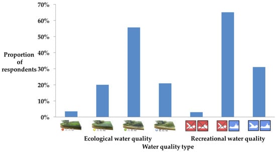
Figure 3.
Visitors perceptions of current water quality at the Yare.
Within Table 6 we saw that where V0 was set to the lowest water quality level, WTP estimates, derived from the CL model, were much higher than if we used respondents’ perceptions of water quality as the baseline upon which to calculate welfare estimates. It was important that we used the correct level for V0 to produce meaningful valuations: if V0 was systematically set to the lowest water quality level, WTP estimates would be potentially overestimated.
Table 6.
WTP of Yare visitors (excluding rowers and swimmers) per km of improvement, per household, per year, accounting for perceived water quality.
4. Discussion
This research disentangles and examines the relationships between ecological and recreational sources of value, thereby allowing decision makers to better understand the consequences of adopting alternative investment strategies that favour either ecological, recreational or a mix of benefits. To do this, this research has used attribute based valuation methods and a broad survey design to analyze the way in which individuals regard the recreational and environmental functions of rivers. We present two complementary models that examine different aspects of the same data.
With regard to the question of who cares about river water quality, our results were stable over the alternative choice models specifications, confirming significant heterogeneity in water quality preferences across the sample of respondents. Clearly the answer to ‘Who cares?’ depends on who is being asked, and asked for what reason. Previous research led us to expect that recreational water users would have higher expectations from water quality in order to fully enjoy their activities and would place greater value on higher recreational water quality. This expectation was confirmed within our CL results, which provided an overview of the water quality preferences of different recreational users and infrequent visitors/non-users within the general public. The public typically hold higher values for improved ecological quality, rather than recreational enhancements. Similar preference orderings, but at higher levels of willingness to pay, were revealed by anglers. However, other users, such as swimmers and rowers, prioritised recreational over ecological improvements. Other preference predictors were identified, including a correlation between respondents’ WTP and the number of environmental memberships they held, and a clear distance decay in WTP values away from the sites of any proposed investment.
What was more unexpected was the heterogeneity revealed by the LC model, which found three statistically distinct types of respondents. The majority hold a preference for enhanced ecological quality, a minority are motivated by recreational quality improvements, and a yet smaller proportion are ambivalent about the water quality at the Yare.
By demonstrating that positive non-market benefits are likely to accrue from remediation schemes and by improving the probability that those schemes would pass cost-benefit analyses, this research advocates for ongoing policies of river improvement. It also shows that the non-market benefits that may accrue from different types of water quality improvements are nuanced in terms of their environmental impacts, their potential beneficiaries, and by inference, their overall value and policy implications. The WTP measures derived from our research reveal clear differences in preferences between respondent groups, and so, from a policy perspective, enhances the ability of the policy-maker to more fully understand potential non-market benefits and thus produce more accurate cost-benefit analyses. Future CBAs could incorporate the preference heterogeneity exhibited by different sub-samples within the population and weight their estimated non-market utility values accordingly. A similar approach could be taken to account for the impact of distance on respondents’ estimated utility values.
So, what are the implications of this study, and how should the policy and management community react? There are spatial differences in ecological and microbiological pollution concentrations and vectors across UK rivers [56,57]. As the costs and the benefits of remediating that pollution are unequally distributed, it is simply not cost effective to direct scarce financial resources at pollution remediation equally across all rivers. The policy and management communities must be pragmatic, accept that not all riverine pollution can be solved in the short term, and adopt a targeted approach to pollution remediation schemes; an approach that closely examines the net benefits arising from different levels of investment at different locations to ensure that the allocation of scarce resources yields the maximum net benefits. Consequently, it is important that research such as this, demonstrates to policymakers that different remedial measures (aimed at either ecological or microbial water quality improvements) may trigger entirely different benefits and differing levels of market and non-market values. Decision makers need to be able to understand these differences, and be able to access simple, quantifiable data in order to maximise the effectiveness of the limited resources available for river improvements, particularly given the elusive nature of non-market quantification.
What is being increasingly confirmed by recent work (e.g., Metcalfe, et al. [16], the findings of which are reinforced by the research presented here) are that the spatial conditions and patterns pertaining to the non-market benefits that may be available following pollution remediation. Respondents’ spatial relationships to rivers are important, especially when monetizing the total utility of non-market benefits.
Our CL model found that distance decay to be a step function, with a preference boundary at 8 km from the river, and our LC model found distance to be a highly significant determinant of class membership. By revealing spatially explicit distributions of non-market benefits, this research helps to identify the optimal locations and recipients for remediation schemes, and thus help maximise the return on investment.
The preferences of the majority of the respondents were directed at the ecological quality of river water. With this in mind, we should expect proportionately more resources to be targeted towards improving the ecological quality of rivers, and we should also expect the majority of water quality improvements to be made close to, but upstream of, urban areas. There are two main reasons for this expectation. Firstly, improvements close to urban areas would reasonably be expected to encompass the largest numbers of beneficiaries (due to the higher population densities of those urban areas) resulting in relatively higher levels of use and non-use benefit values (remediation measures in isolated rural locations would be expected to have relatively low benefit values, simply because there are very few people in those locations to gain utility from an improvement). Secondly, areas downstream of urban areas are frequently subject to unidirectional pollution discharges from the wastewater treatment facilities that process wastewater originating from those settlements. The costs of installing, or upgrading, wastewater treatment facilities to adequately treat discharges from those urban areas may outweigh the benefits that may arise from the treatment of that wastewater. Much depends on the spatial vagaries of wastewater infrastructure, the relationships of the urban areas to rivers, the location of beneficiaries and the locations of other sources of river pollution.
The underlying rationale of the paper is that, given resource constraints, a focus on identifying and improving those sites which yield the largest net benefits is entirely justified. This in turn requires estimates of the benefits of improvement to set against costs, and our analysis revealed the importance of key parameters (such as user type and their distance from the proposed improvement) in determining those benefits. Failure to identify benefits negates the decision makers’ ability to discriminate between investment options.
The practical way forward with respect to widespread application of benefit appraisal is clarified by considering commonplace approaches towards appraisal of the cost side of any water quality investment. Costs have been estimated from a number of original studies of different rivers and interventions. Cost models are then applied to new potential investments by simply gathering some readily available secondary data including maps of the relevant rivers, and a minimum of on-site measurement (for example, some minimal quality assessment). In effect, a base of cost data gathered from prior investigations of other rivers is then used to estimate costs for interventions on other rivers. This process forms the basis for practice on the benefits side. Our study provides a detailed analysis of the benefits of water quality improvements across different user groups living at different distances from the studied river. These parameters allow us to extrapolate results to other rivers, again through the application of readily available secondary data, including maps of the relevant rivers. Of course, just as it would be unwise to estimate costs for all other rivers from those incurred at a single river, one would want to conduct a number of further primary benefit valuation studies prior to combining these within a transferable benefit valuation model. We set out the principles for such an exercise elsewhere [10]; these are principles which the relevant decision makers have for some time accepted as the desired and practical approach to benefit valuation across multiple rivers and waterways [12,58,59,60,61].
4.1. Research Limitations
Other variables to capture the potential effect of distance on respondents’ preferences were explored (e.g., specifying distance as a continuous variable, to obtain true distance decay, rather than a preference boundary based on the mean distance respondents live from the survey river), but these proved unsatisfactory. It might be that with a larger sample size, and more variability in respondents’ distances from the survey river, results would differ.
Several of the groups of socio-economic variables within the CL produced coefficients with wide confidence intervals, which we believe was due to small sample size (Rowers and swimmers, in particular, proved to be particularly ‘hard to reach’ respondents; they were reticent about being interviewed, despite advertisements being placed within club newsletters). Consequently, some of the socio-economic coefficients were insignificant and cannot be taken at face value. However, these insignificant variables are useful as a guide to identify trends in the data. Despite this caveat, many of the socio-economic variables were significant, particularly those that provided the highest utility for the different types of recreational users.
By choosing to minimise experimental complexity to focus on respondents’ trade-offs between only ecological quality, recreational quality and price, it may be argued that this research has missed the opportunity to explore other facets of water quality (e.g., contamination by industrial pollutants), or to explore respondents’ preferences for potential water remediation options (e.g., build a wastewater treatment facility at point A or B). This limitation makes direct comparison with other research, e.g., Doherty et al. [14] and Hanley et al. [15] more problematic.
The transferability of our research findings has not been explored here. Given the small overall sample size and the low numbers of respondents participating in river-based recreation activities, it was not prudent to perform out-of-sample testing. However, the model function contains distance, a key element for transferability, and the dataset includes other useful variables, such as income. Previous research [24] has suggested that in most cases, differences between WTP estimates obtained by different methods (e.g., travel cost or contingent valuation) are larger than differences due to dissimilar river characteristics: when multiple studies are available, welfare estimates for rivers that have similar characteristics, but are based on different methods, consistently result in larger errors than transfers across space, keeping the method constant. With this in mind, it may be beneficial in the future to assess our results against those obtained by studies that use similar methods and were undertaken at rivers with similar characteristics. We should be fairly confident that the results presented here offer insights into the patterns of respondents’ utility preferences in other similar areas.
4.2. Future Research
Like most research, this work has identified new research avenues. Our perception-based WTP estimates were similar to the WTP estimates obtained from other recent UK studies, for example, Metcalfe et al. [16], Hanley et al. [15] and Glenk et al. [11]. A meta-analysis of utility values and/or assessment of transfer error values from these and other studies may be useful, particularly if the goal is to produce spatially transferable models.
A further research avenue could be to map the spatial boundaries of our utility estimates of the non-market benefits arising from water quality improvements against empirical water quality data, in order to improve our understanding of the optimal locations in which the non-market benefits from river water quality remediation schemes could be maximised.
Supplementary Materials
The questionnaire and showcards used for the survey are available online at www.mdpi.com/2073-4441/9/8/621/s1.
Acknowledgments
Funding for this research was provided by SEER (the Social and Environmental Economic Research project, funded by the ESRC; Ref: RES-060-25-0063) and ChREAM (the Catchment hydrology, Resources, Economics and Management project, funded by the joint ESRC, BBSRC and NERC Rural Economy and Land programme; Ref: RES-227-25-0024). ESRC support for Danyel Hampson (grant number ES/F023693/1} is gratefully acknowledged. All subjects gave their informed consent for inclusion before they participated in the study. The study was conducted in accordance with the Declaration of Helsinki, and the protocol was approved by the Ethics Committee of University of East Anglia (RES-227-25-0024). No funds were received to cover the costs of publishing in open access. We are grateful to three anonymous referees for their helpful advice regarding the preparation of this paper.
Author Contributions
Danyel I. Hampson and Ian J. Bateman conceived and designed the research and questionnaire design; Dan Rigby developed the choice experiment design; Danyel I. Hampson carried out the fieldwork; Danyel I. Hampson generated and analyzed the conditional logit models; Ian J. Bateman and Silvia Ferrini supervised and moderated the conditional logit analysis; Danyel I. Hampson generated and analyzed the latent class models; Silvia Ferrini supervised and moderated the latent class analysis; Dan Rigby provided supplementary analysis on the latent class data; Silvia Ferrini reanalysed the data to reflect respondents’ perceptions of water quality; Danyel I. Hampson and Silvia Ferrini wrote the paper, with contributions from Ian J. Bateman and Dan Rigby.
Conflicts of Interest
The authors declare no conflict of interest. The founding sponsors had no role in the design of the study; in the collection, analyses, or interpretation of data; in the writing of the manuscript, and in the decision to publish the results.
References
- Council of the European Communities (CEC). Council directive 2000/60/EC of the European Parliament and of the Council of 23 October 2000 establishing a framework for community action in the field of water policy. Off. J. Eur. Community 2000, L327, 1–72. [Google Scholar]
- Defra. Overall Impact Assessment for the Water Framework Directive (EC 2000/60/EC); Department for Environment, Food and Rural Affairs: London, UK, 2008.
- Boardman, A.E.; Greenburg, D.H.; Vining, A.R.; Weimer, D. Cost-Benefit Analysis: Concepts and Practice, 4th ed.; Pearson Education, Inc.: Upper Saddle River, NJ, USA, 2014. [Google Scholar]
- H.M. Treasury. The Green Book: Appraisal and Evaluation in Central Government; The Stationary Office: London, UK, 2003.
- Schaafsma, M.; Ferrini, S.; Harwood, A.R.; Bateman, I.J. The first United Kingdom’s national ecosystem assessment and beyond. In Water Ecosystem Services: A Global Perspective; Martin-Ortega, J., Ferrier, R.C., Gordon, I.J., Khan, S., Eds.; Cambridge University Press: Cambridge, UK, 2015; pp. 73–81. [Google Scholar]
- Birol, E.; Karousakis, K.; Koundouri, P. Using economic valuation techniques to inform water resources management: A survey and critical appraisal of available techniques and an application. Sci. Total Environ. 2006, 365, 105–122. [Google Scholar] [CrossRef] [PubMed]
- Brouwer, R.; Martin-Ortega, J.; Dekker, T.; Sardonini, L.; Andreu, J.; Kontogianni, A.; Skourtos, M.; Raggi, M.; Viaggi, D.; Pulido-Velazquez, M.; et al. Improving value transfer through socio-economic adjustments in a multicountry choice experiment of water conservation alternatives. Aust. J. Agric. Resour. Econ. 2015, 59, 458–478. [Google Scholar] [CrossRef]
- Andreopoulos, D.; Damigos, D.; Comiti, F.; Fischer, C. Public preferences for climate change adaptation policies in Greece: A choice experiment application on river uses. In Agricultural Cooperative Management and Policy; Zopounidis, C., Kalogeras, N., Mattas, K., Van Dijk, G., Baourakis, G., Eds.; Springer: Cham, Switzerland, 2014; pp. 163–178. [Google Scholar]
- Johnston, R.J.; Boyle, K.J.; Adamowicz, W.; Bennett, J.; Brouwer, R.; Cameron, T.A.; Hanemann, W.M.; Hanley, N.; Ryan, M.; Scarpa, R.; et al. Contemporary Guidance for Stated Preference Studies. J. Assoc. Environ. Resour. Econ. 2017, 4, 319–405. [Google Scholar] [CrossRef]
- Bateman, I.J.; Brouwer, R.; Ferrini, S.; Schaafsma, M.; Barton, D.N.; Dubgaard, A.; Hasler, B.; Hime, S.; Liekens, I.; Navrud, S.; et al. Making benefit transfers work: Deriving and testing principles for value transfers for similar and dissimilar sites using a case study of the non-market benefits of water quality improvements across Europe. Environ. Resour. Econ. 2011, 50, 356–387. [Google Scholar] [CrossRef]
- Glenk, K.; Lago, M.; Moran, D. Public preferences for water quality improvements: Implications for the implementation of the EC Water Framework Directive in Scotland. Water Policy 2011, 13, 645–662. [Google Scholar] [CrossRef]
- World Health Organization. Guidelines for Safe Recreational Water Environments; Volume 1: Coastal and Fresh Waters; World Health Organization: Geneva, Switzerland, 2003. [Google Scholar]
- Crowther, J.; Hampson, D.I.; Bateman, I.J.; Kay, D.; Posen, P.E.; Stapleton, C.M.; Wyer, M.D. Generic modelling of faecal indicator organism concentrations in the UK. Water 2011, 3, 682–701. [Google Scholar] [CrossRef]
- Doherty, E.; Murphy, G.; Hynes, S.; Buckley, C. Valuing ecosystem services across water bodies: Results from a discrete choice experiment. Ecosyst. Serv. 2014, 7, 89–97. [Google Scholar] [CrossRef]
- Hanley, N.; Wright, R.E.; Alvarez-Farizo, B. Estimating the economic value of improvements in river ecology using choice experiments: An application to the water framework directive. J. Environ. Manag. 2006, 78, 183–193. [Google Scholar] [CrossRef] [PubMed]
- Metcalfe, P.; Baker, W.; Andrews, K.; Atkinson, G.; Bateman, I.J.; Butler, S.; Carson, R.; East, J.; Gueron, Y.; Sheldon, R.; et al. An assessment of the nonmarket benefits of the water framework directive for households in England and Wales. Water Resour. Res. 2012, 48, WO3526. [Google Scholar] [CrossRef]
- Bateman, I.J.; Mace, G.M.; Fezzi, C.; Atkinson, G.; Turner, K. Economic analysis for ecosystem service assessments. Environ. Resour. Econ. 2011, 48, 177–218. [Google Scholar] [CrossRef]
- Natural England. Catchment Sensitive Farming: Anglian River Basin District Strategy 2016 to 2021; Natural England: York, UK, 2016.
- Environment Agency. The Broadland Rivers Management Catchment; Environment Agency: Bristol, UK, 2014.
- Vaughan, W.J. The Water Quality Ladder. In An Experiment in Determining Willingness to Pay for National Water Quality Improvements; Mitchell, R.C., Carson, R.T., Eds.; Report to the US Environmental Protection Agency; Resources for the Future, Inc.: Washington, DC, USA, 1981; Appendix II. [Google Scholar]
- Bateman, I.J.; Brouwer, R.; Davies, H.; Day, B.H.; Deflandre, A.; Falco, S.D.; Georgiou, S.; Hadley, D.; Hutchins, M.; Jones, A.P.; et al. Analysing the agricultural costs and non-market benefits of implementing the water framework directive. J. Agric. Econ. 2006, 57, 221–237. [Google Scholar] [CrossRef]
- Hime, S.; Bateman, I.J.; Posen, P.; Hutchins, M. A Transferable Water Quality Ladder for Conveying Use and Ecological Information within Public Surveys; CSERGE Working Paper EDM 09-01; University of East Anglia: Norwich, UK, 2009. [Google Scholar]
- UK Technical Advisory Group. Water Framework Directive Phase 1 Report—Environmental Standards and Conditions for Surface Waters; UK Technical Advisory Group: London, UK, 2008. [Google Scholar]
- Ferrini, S.; Schaafsma, M.; Bateman, I.J. Revealed and stated preference valuation and transfer: A within-sample comparison of water quality improvement values. Water Resour. Res. 2014, 50, 4746–4759. [Google Scholar] [CrossRef]
- Konishi, Y.; Coggins, J.S. Environmental risk and welfare valuation under imperfect information. Resour. Energy Econ. 2008, 30, 150–169. [Google Scholar] [CrossRef]
- Happs, J. Constructing an understanding of water-quality: Public perceptions and attitudes concerning three different water-bodies. Res. Sci. Educ. 1986, 16, 208–215. [Google Scholar] [CrossRef]
- Poor, P.J.; Boyle, K.J.; Taylor, L.O.; Bouchard, R. Objective versus subjective measures of water clarity in hedonic property value models. Land Econ. 2001, 77, 482–493. [Google Scholar] [CrossRef]
- Rigby, D.; Alcon, F.; Burton, M. Supply Uncertainty and the Economic Value of Irrigation Water. Eur. Rev. Agric. Econ. 2010, 37, 97–117. [Google Scholar] [CrossRef]
- Train, K.; Hensher, D.; Shore, N. Households’ Willingness to Pay for Water Service Attributes. Environ. Resour. Econ. 2005, 32, 509–531. [Google Scholar] [CrossRef]
- Ferrini, S.; Scarpa, R. Designs with a-priori information for nonmarket valuation with choice experiments: A Monte Carlo study. J. Environ. Econ. Manag. 2007, 53, 342–363. [Google Scholar] [CrossRef]
- ChoiceMetrics PTY Ltd. NGene Handbook for Version 1.1. 2012. Available online: http://www.choice-metrics.com (accessed on 24 April 2017).
- Samples, K.C.; Dixon, J.A.; Gowen, M.M. Information Disclosure and Endangered Species Valuation. Land Econ. 1986, 62, 306–312. [Google Scholar] [CrossRef]
- Bailar, B.; Bailey, L.; Stevens, J. Measures of interviewer bias and variance. J. Mark. Res. 1977, 14, 337–343. [Google Scholar] [CrossRef]
- Hensher, D.A.; Rose, J.M.; Greene, W.H. Applied Choice Analysis: A Primer; Cambridge University Press: Cambridge, UK, 2005. [Google Scholar]
- McFadden, D. Conditional logit analysis of qualitative choice behavior. In Frontiers in Econometrics, 1st ed.; Zarembka, P., Ed.; Academic Press: New York, NY, USA, 1974; pp. 105–142. [Google Scholar]
- Luce, R.D. Individual Choice Behavior: A Theoretical Analysis; John Wiley and Sons, Inc.: New York, NY, USA, 1959. [Google Scholar]
- McFadden, D.; Train, K. Mixed MNL models for discrete response. J. Appl. Econ. 2000, 15, 447–470. [Google Scholar] [CrossRef]
- Morey, E.R.; Thacher, J.; Breffle, W. Using angler characteristics and attitudinal data to identify environmental preference classes: A latent-class model. Environ. Resour. Econ. 2006, 34, 91–115. [Google Scholar] [CrossRef]
- Kemperman, A.D.; Timmermans, H.J. Heterogeneity in urban park use of aging visitors: A latent class analysis. Leis. Sci. 2006, 28, 57–71. [Google Scholar] [CrossRef]
- McFadden, D. The choice theory approach to market research. Mark. Sci. 1986, 5, 275–297. [Google Scholar] [CrossRef]
- Greene, W.H.; Hensher, D.A. A latent class model for discrete choice analysis: Contrasts with mixed logit. Transp. Res. B 2003, 37, 681–698. [Google Scholar] [CrossRef]
- Hess, S.; Ben-Akiva, M.; Gopinath, D.; Walker, J. Advantages of Latent Class Over Continuous Mixture of Logit Models; Institute for Transport Studies, Working Paper; University of Leeds: Leeds, UK, 2011. [Google Scholar]
- Provencher, B.; Moore, R. A discussion of ‘using angler characteristics and attitudinal data to identify environmental preference classes: A latent-class model’. Environ. Resour. Econ. 2006, 34, 117–124. [Google Scholar] [CrossRef]
- Boxall, P.C.; Adamowicz, W.L. Understanding heterogeneous preferences in random utility models: A latent class approach. Environ. Resour. Econ. 2002, 23, 421–446. [Google Scholar] [CrossRef]
- Shonkwiler, J.S.; Shaw, W.D. A finite mixture approach to analyzing income effects in random utility models: Reservoir recreation along the Columbia river. In The New Economics of Outdoor Recreation; Hanley, N., Shaw, W.D., Wright, R.E., Eds.; Edward Elgar Publishing: Northampton, UK, 2003; pp. 268–278. [Google Scholar]
- Morey, E.R.; Thacher, J.A. Using Choice Experiments and Latent-Class Modeling to Investigate and Estimate How Academic Economists Value and Trade Off the Attributes of Academic Positions; Working Paper; University of Colorado: Boulder, CO, USA, 2012. [Google Scholar]
- Hanemann, W.M. Welfare evaluations in contingent valuation experiments with discrete responses. Am. J. Agric. Econ. 1984, 66, 332–341. [Google Scholar] [CrossRef]
- Hynes, S.; Hanley, N.; Scarpa, R. Effects on welfare measures of alternative means of accounting for preference heterogeneity in recreational demand models. Am. J. Agric. Econ. 2008, 90, 1011–1027. [Google Scholar] [CrossRef]
- Krinsky, I.; Robb, L. On approximating the statistical properties of elasticities. Rev. Econ. Stat. 1986, 68, 715–719. [Google Scholar] [CrossRef]
- British Rowing. Governance. Available online: https://www.britishrowing.org/about-us/governance/ (accessed on 14 August 2017).
- Environment Agency. Public Attitudes to Angling 2010; Environment Agency: Bristol, UK, 2010.
- StataCorp, L.P. Stata Statistical Software, Version 13.1. 2013. Available online: https://www.stata.com (accessed on 14 April 2017).
- Bateman, I.J.; Day, B.H.; Georgiou, S.; Lake, I. The aggregation of environmental benefit values: Welfare measures, distance decay and total WTP. Ecol. Econ. 2006, 60, 450–460. [Google Scholar] [CrossRef]
- Statistical Innovations. Latent GOLD, Version 5.1. 2014. Available online: https://www.statisticalinnovations.com (accessed on 14 April 2017).
- Hanley, N.; Bell, D.; Alvarez-Farizo, B. Valuing the benefits of coastal water quality improvements using contingent and real behaviour. Environ. Resour. Econ. 2003, 24, 273–285. [Google Scholar] [CrossRef]
- Hampson, D.; Crowther, J.; Bateman, I.J.; Kay, D.; Posen, P.; Stapleton, C.; Wyer, M.; Fezzi, C.; Jones, P.; Tzanopoulos, J. Predicting microbial pollution concentrations in UK rivers in response to land use change. Water Res. 2010, 44, 4748–4759. [Google Scholar] [CrossRef] [PubMed]
- Haygarth, P.; Granger, S.; Chadwick, D.; Shepherd, M.; Fogg, P. A Provisional Inventory of Diffuse Pollution Losses. ADAS Report for Defra; ADAS: Wolverhampton, UK, 2005. [Google Scholar]
- Eftec. Benefits Assessment Guidance: User Guide; Report to the Environment Agency for England and Wales; Economics for the Environment Consultancy Ltd.: London, UK, 2012. [Google Scholar]
- Environment Agency. Guidance: Assessment of Benefits for Water Quality and Water Resources Schemes in the PR04 Environment Programme. 2003. Available online: http://www.environment-agency.gov.uk/business/sectors/37305.aspx (accessed on 15 August 2017).
- Environment Agency. Valuing Environmental Benefits. External Briefing Note; Environment Agency, 2013a. Available online: http://www.thames21.org.uk/wp-content/uploads/2013/12/NWEB-Briefing-Notes.pdf (accessed on 15 August 2017).
- Environment Agency. Water Appraisal Guidance; Assessing Costs and Benefits for River Basin Management Planning. Environment Agency, 2013b. Available online: http://www.ecrr.org/Portals/27/Publications/Water%20Appraisal%20Guidance.pdf (accessed on 15 August 2017).
© 2017 by the authors. Licensee MDPI, Basel, Switzerland. This article is an open access article distributed under the terms and conditions of the Creative Commons Attribution (CC BY) license (http://creativecommons.org/licenses/by/4.0/).