A New Procedure for Determining Monthly Reservoir Storage Zones to Ensure Reliable Hourly Hydropower Supply

Abstract

The uncertainty of natural inflows and market behavior challenges ensuring a reliable power balance in hydropower-dominated electricity markets. This study proposes a novel framework integrating hourly load balancing on typical days into a monthly scheduling model solved with Gurobi11.0.1 to evaluate demand-met reliability across storage and inflow states. By employing total storage as a system state to reduce dimensional complexity and simulating future runoff scenarios based on current inflows, the method performs multi-year statistical simulations to assess reliability over the following year. Applied to a system of 39 hydropower reservoirs in China, the case studies of present models and procedures suggest: (1) controlling reservoir storage levels during the dry season is crucial for ensuring the power demand-met rate in the following year, with May being the most critical month; (2) the power demand-met rate does not monotonically increase with higher storage levels—there is an optimal storage level that maximizes the demand-met rate; and (3) June and October offer the greatest flexibility in storage adjustment to achieve the highest demand-met reliability.

1. Introduction

Hydropower reservoir operation has long been studied in water resources management because of its critical role in meeting energy demand and ensuring a reliable electricity supply, especially in hydropower-dominated systems. Cascaded hydropower reservoirs are often jointly operated optimally to balance hydropower, water storage, and environmental requirements [1,2]. Seasonal variability, climate change, and extreme weather events bring about the uncertainty of natural inflows. The unpredictability makes it challenging to predict future water resource availability and makes water release decisions for hydropower generation complex. This has added considerable complexity to reservoir management [3,4]. While references [5,6,7,8,9] effectively address uncertainty in inflow modeling, they lack a focus on power demand-met reliability. Despite the progress made in risk management strategies by integrating probabilistic methods and runoff forecasting techniques into optimization models and decision-supporting tools. However, ensuring power supply reliability under uncertain inflows remains a persistent and demanding challenge for power system operators [7,8]. Existing research often lacks frameworks that explicitly target power demand-met reliability while considering multi-reservoir systems under uncertainty.

Because of their simplicity and ease of use, operational rules are widely used to guide hydropower reservoirs’ monthly dynamic storage control when the future inflow is uncertain. Adaptable to changing system states, these operational rules are pre-defined release and storage decision guidelines based on historical inflows, forecast conditions, and demand patterns, helpful in improving water resources utilization and power supply reliability [9,10]. However, these rules are often static and fail to account for dynamic changes in inflow and demand, creating a research gap in real-time adaptability.

The development and application of operational rules for hydropower reservoir management have been extensively studied [2,11]. Much of the earlier work focuses on optimizing strategies for single-reservoir systems to maximize energy production while considering competing objectives, such as flood control and water supply [12,13]. Previous efforts were often made to deal with single-reservoir systems and failed to address the complexity of multi-reservoir ones, especially when involving cascaded reservoirs, which must be coordinated to optimize hydropower generation and meet downstream demands [14,15]. References [14,16] highlight dimensional challenges but do not tackle short-term load balancing. Therefore, further research is required to extend these operating rules to multi-reservoir systems. However, dimensional difficulties become a primary concern when dealing with more controllable reservoirs, making optimizing storage, release, and hydropower generation computationally challenging across multiple interconnected reservoirs under uncertain inflow scenarios.

An operational rule is a function of system states, typically relying on current reservoir storage levels and expected inflows to ensure decisions reflect the system’s most up-to-date status [17,18]. These rules are commonly developed monthly for long-term planning, assuming reservoir operations can be periodically adjusted based on seasonal and inter-annual variations [19,20]. While this monthly framework is helpful for long-term assessments, it is often too coarse for real-time operation. Power supply must be balanced on an hourly scale to meet fluctuating daily demand, and this mismatch between monthly averages and hourly performance creates challenges for power supply reliability [21,22]. This mismatch underscores a specific gap in the field: the need for a methodology that integrates hourly fluctuations into a long-term planning framework. A finer temporal resolution is needed to bridge the gap between long-term planning and short-term operational needs.

Employing charts to represent operational rules is a common engineering practice, where storage levels or zones are defined to target a constant, firm hydropower output, and decision-making is simplified by using storage as the only state variable, making it popular for its ease of use and intuitive approach [23,24]. These charts serve as operational rules, determining specific water levels at the beginning of each month to guide a hydropower reservoir in releasing and refilling to meet hydropower production targets. The conventional charts, however, are often calibrated with limited representative inflow scenarios. This may not fully account for the variability of natural inflows [25,26]. Thus, these rules may lead to suboptimal solutions since they cannot fully account for the inflow uncertainty and dynamic changes [27,28]. The rule curves have advantages in simplicity when implemented but cannot ensure their adaptability to various real-time conditions of unpredictable inflows by relying on a few inflow scenarios. A broader range of inflow scenarios is needed to ensure adaptability and reliability under diverse conditions.

This work considers the total storage capacity of the cascade system as a single decision variable. Then, it was optimized and allocated to various reservoirs, simplifying the management of large-scale hydropower systems. The procedure determines the demand-met rate for different system states, simulating enough years of historical inflow scenarios and accounting for dynamic power demands at monthly and hourly scales. A typical day is chosen each month to capture detailed hourly demand variations. The demand-met rate depends on both storage and inflow conditions, and the resulting storage corridor functions as an operational rule/chart that ensures the reliable fulfillment of hourly power demands from a long-term standpoint. When simulated under various inflow scenarios, this model incorporates hourly load balances into a monthly formulation to ensure water allocation is more closely aligned with fluctuating load demands. This work offers a practical framework adaptable to a real-time system state to provide a consistent hydropower supply under diverse conditions: (1) targeting power demand-met reliability in a mid-to-long-term hydro scheduling; (2) integrating hourly load balancing into long-term scheduling to bridge the gap between planning and real-time operations; and (3) reducing dimensional complexity by employing the total storage as a state variable.

2. An Hourly Balance in Monthly Scheduling Problem

The monthly scheduling problem over a year usually aims to ensure maximum firm power output and total power output. This can ensure power is out during the dry season and maximize the power output efficiency. On this basis, this paper also added the relevant goal of maximizing the load met rate. The rate is measured by a slack variable, mathematically expressed as:

$$\mathrm{m}\mathrm{i}\mathrm{n}{W}_1\sum _{m=0}^{11}\sum _{t=0}^{23}S{L}_{mt}-\left[W_2·F+W_3\sum _{i=1}^{NR}\sum _{m=0}^{11}{P}_{im}+W_4\sum _{m=0}^{11}\underset{m}{\overset{\mathrm{e}\mathrm{x}\mathrm{t}\mathrm{r}\mathrm{a}}{P}}\right]$$

(1)

where NR = the total number of hydropower reservoirs; F = the firm power output in MW; i and m = subscripts for reservoirs and months; $P_{im}$= hydropower out in MW on average of hydroplant i over month m; $P_m^{\mathrm{e}\mathrm{x}\mathrm{t}\mathrm{r}\mathrm{a}}$ = an additional hydropower output in MW that can be constantly supplied every hour during the typical day of month m; $S{L}_{mt}$ = the shortage to meet the power demand in hour t on a typical day of month m; and W₁, W₂, W₃, and W₄ = weights assigned differently in magnitude to prioritize the sub-objectives, with W₄>> W₁>> W₂ = W₃.

The constraints include the following:

(1)

The water balance:

$$V_{i,m+1}=V_{im}+(Q_{im}^{\mathrm{com}}-Q_{im}^{\mathrm{out}})·∆m$$

(2)

$$Q_{im}^{\mathrm{com}}=Q_{im}^{\mathrm{l}\mathrm{o}\mathrm{c}}+\sum _{k\in \Omega \left(i\right)}{Q}_{km}^{\mathrm{o}\mathrm{u}\mathrm{t}}$$

(3)

where $V_{im}$ = the storage capacity in hm³ of reservoir i at the beginning of month m; $Q_{im}^{\mathrm{com}}$ = the inflow in m³/s of i reservoir in month m; $Q_{im}^{\mathrm{out}}$ is the outflow in m³/s of i reservoir in month m; $Q_{im}^{\mathrm{l}\mathrm{o}\mathrm{c}}$ is the local inflow in m³/s of reservoir j in month m; and $\Omega \left(i\right)$ is the set of reservoirs immediately upstream of reservoir i.

(2)

Upper and lower bounds on storage and release:

$$V_i^{\mathrm{m}\mathrm{i}\mathrm{n}}\left(Z_i^{\mathrm{m}\mathrm{i}\mathrm{n}}\right)\le V_{im}\le V_i^{\mathrm{m}\mathrm{a}\mathrm{x}}\left(Z_i^{\mathrm{m}\mathrm{a}\mathrm{x}}\right)$$

(4)

$$Q_i^{\mathrm{m}\mathrm{i}\mathrm{n}}\le Q_{im}^{\mathrm{out}}\le Q_i^{\mathrm{m}\mathrm{a}\mathrm{x}}$$

(5)

where $V_i^{\mathrm{m}\mathrm{i}\mathrm{n}}(·)$ = the minimum storage capacity in hm³ of reservoir i, which is determined by the minimum water level $Z_i^{\mathrm{m}\mathrm{i}\mathrm{n}}$ in meters, usually the dead storage level; $V_i^{\mathrm{m}\mathrm{a}\mathrm{x}}(·)$ = the maximum storage capacity in hm³ of reservoir i, determined by the maximum water level $Z_i^{\mathrm{m}\mathrm{a}\mathrm{x}}$ in meters; and $Q_i^{\mathrm{m}\mathrm{i}\mathrm{n}}$ and $Q_i^{\mathrm{m}\mathrm{a}\mathrm{x}}$ = the minimum and maximum outflows in m³/s of reservoir i, respectively.

(3)

Periodical and sustainable conditions, assuming the end of a year is the beginning of the year:

$$V_{i,0}=V_{i,12}$$

(6)

where V_i0 = the storage in hm³ of reservoir i at the beginning of the scheduling horizon.

(4)

Overall storage state is enforced as:

$$\sum _{i=1}^{NR}{V}_{i,0}={\mathrm{S}\mathrm{V}}_0$$

(7)

where SV₀ = the total storage given as a boundary condition at the beginning of the scheduling horizon.

The total initial storage capacity of all reservoirs is used as a state variable to reduce the dimensionality of the solution. In order to obtain all values in the state space, all possible total storage capacity states were incorporated into the calculation.

(5)

The hydropower output constrained by available outflow:

$$P_{im}\le a_{ik}^{\left(1\right)}{\overline{V}}_{im}+b_{ik}^{\left(1\right)}{Q}_{im}^{\mathrm{o}\mathrm{u}\mathrm{t}}+c_{ik}^{\left(1\right)}$$

(8)

$${\overline{V}}_{im}={\displaystyle \frac{V_{im}+V_{i,m+1}}{2}}$$

(9)

where the hydropower output is linearized using a three-triangle-based global concaving method [29], with $a_{ik}^{\left(1\right)}$, $b_{ik}^{\left(1\right)}$, and $c_{ik}^{\left(1\right)}$ being the parameters that define the k^th triangle surface of the hydropower output function of reservoir I, and ${\overline{V}}_{im}$ being the average storage of reservoir i in month m.

Specifically, the three-triangle-based global condensing method usually does not consider spillage during optimization. However, after the optimization is completed, based on the scheduling results and maximum generation discharge data, the outflow is redistributed into two parts: generation discharge and spillage flow, in order to correct the power output.

(6)

Firm hydropower output:

$$\sum _{i=1}^{NR}{P}_{im}\ge F$$

(10)

(7)

As illustrated in Figure 1, power demands are hourly balanced on a typical day of the month,

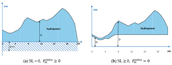Figure 1. Hourly power balance during a typical day.

$${\sum }_{i=1}^{NR}{P}_{imt}+S{L}_{mt}-P_m^{\mathrm{e}\mathrm{x}\mathrm{t}\mathrm{r}\mathrm{a}}=D_{mt}$$

(11)

with the generating capacity enforced as:

$$P_{imt}\le a_{ik}^{\left(2\right)}{\overline{V}}_{im}+b_{ik}^{\left(2\right)}{Q}_{im}^{\mathrm{o}\mathrm{u}\mathrm{t}}+c_{ik}^{\left(2\right)}$$

(12)

and energy balanced during a month:

$${\displaystyle \frac{1}{24}}\sum _{t=0}^{23}{P}_{imt}=P_{im}$$

(13)

where $a_{ik}^{\left(2\right)}$, $b_{ik}^{\left(2\right)},$ and $c_{ik}^{\left(2\right)}$ = parameters that define the k^th triangle surface of the generating capacity function of reservoir i; $P_{imt}$ = power output in MW of hydroplant i in hour t of the typical day in month m; $D_{mt}$ = the power demand in MW in hour t of the typical day of month m; and ${SL}_{mt}$ = shortage in MW to meet the power demand in hour t of a typical day of month m, serving in the model as a slack variable, which equals to or greater than 0 to indicate whether the power demand is met. At the hourly scale, power output capacity needs to be limited in order to achieve more accurate power balance, and at the monthly scale, this limitation will be evenly distributed.

3. Solution Procedure

A monthly scheduling linear programming model considering typical daily and hourly load balancing is constructed with Equation (1) as the objective function and Equations (2)–(13) as constraints. This study uses the Gurobi optimizer software to solve the model. Figure 2 shows the procedure to estimate the power demand-met rate for a given system state, represented by the total storage (SV₀) and inflow (SQ₀) of cascaded hydropower reservoirs, which is divided across individual reservoirs to alleviate the dimensional difficulties using inflow ratios. Historical inflows are scaled to generate scenarios that reflect each reservoir’s current inflow state. Then, the monthly hydropower scheduling with hourly power balances is simulated yearly for all inflow scenarios to determine the power demand-met rate by the above linear programming model. Each month, the procedure is applied to all the representative states to estimate their respective demand-met rate.

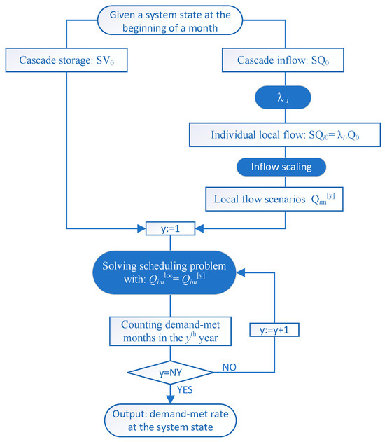
Figure 2. Procedure to determine the demand-met rate at a system state.

3.1. Inflow Scenarios

The runoff correlates strongly between tributaries with similar geographical and natural conditions. To alleviate the dimensional difficulty and simplify the use of operational charts, this study uses the total inflow into the whole cascade system as the runoff state, which is allocated into individual reservoirs according to the annual average runoff of each tributary, determined as:

$${SQ}_{i0}={\lambda }_i·{SQ}_0$$

(14)

where SQ₀ = the total inflow in m³/s into the hydropower system in the upcoming/first month; SQ_i0 = the local natural inflow in m³/s into reservoir i in the forthcoming month; and ${\lambda }_i$ = the proportional ratio of local inflow into reservoir i to the total inflow into the system.

This work assumes that there are inflow scenarios that could equally possibly occur in the upcoming year, and the distribution of these scenarios is determined by the current inflow conditions, represented by the inflow observed in the current month. Here, a sample of local flows into a reservoir is generated by scaling the historically observed local inflows to reflect the current inflow status, mathematically determined as:

$$Q_{im}^{\left[y\right]}={\displaystyle \frac{{SQ}_{i0}}{{\widehat{Q}}_{i0}^{\left[y\right]}}}{\widehat{Q}}_{im}^{\left[y\right]}$$

(15)

where $Q_{im}^{\left[y\right]}$= local inflow in m³/s of reservoir i in month m of the y^th scenario/year, and ${\widehat{Q}}_{im}^{\left[y\right]}$= local inflow in m³/s of reservoir i historically observed in month m of year y.

3.2. Demand-Med Rate

Based on a monthly runoff scenario over a year, the water levels at the start and end of the year are fixed to the predetermined states. After simulating the optimization, whether the hourly load demands are met can be assessed for each month with the following expression:

$${\mu }_m^{\left[y\right]}=\left\{\begin{array}{cc}1& \mathrm{i}\mathrm{f}{\displaystyle \sum _t}{SL}_{mt}=0\\ 0& \mathrm{o}\mathrm{t}\mathrm{h}\mathrm{e}\mathrm{r}\mathrm{w}\mathrm{i}\mathrm{s}\mathrm{e}\end{array}\right.$$

(16)

Thus, the load demand-med rate (DMR) can be statistically derived after running simulation scheduling over multiple years with the following expression:

$$\mathrm{D}\mathrm{M}\mathrm{R}\left({SV}_0,{SQ}_0\right)={\displaystyle \frac{{\sum }_{y=1}^{NY}{\vartheta }^{\left[y\right]}}{NY}},$$

(17)

which can be determined for all representative discrete states every month, with

$${\vartheta }^{\left[y\right]}=\left\{\begin{array}{cc}1& \mathrm{i}\mathrm{f}{\sum }_{m=0}^{11}{\mu }_m^{\left[y\right]}\ge 1\\ 0& \mathrm{o}\mathrm{t}\mathrm{h}\mathrm{e}\mathrm{r}\mathrm{w}\mathrm{i}\mathrm{s}\mathrm{e}\end{array}\right.$$

(18)

to determine whether the power demand is met in the y^th year.

4. Case Studies

4.1. Engineering Background

This work applies the model and program to 39 major hydropower stations, as shown in Figure 3. These hydropower stations are in the southwest of China, which is an important water source energy base with abundant water resources and large river drops. These power stations are established on five rivers, marked as A, B, C, D, and E, which play a crucial role in regional hydropower and water resource management. The cascade hydropower stations on River B are particularly important for regulating and controlling seasonal inflows. Moreover, 22 out of 39 reservoirs possess seasonal or over-seasonal regulation capabilities, allowing for optimization on a monthly scale over a year.

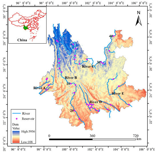
Figure 3. Location of rivers and hydropower reservoirs.

Table 1 shows the main parameters of four representative hydropower reservoirs, identified by Reservoirs 1#, 2#, 3#, and 4#. Based on the runoff distribution, the year can be divided into dry and flood seasons. In these five basins, the flood season typically occurs from June to October, while the dry season lasts from November to May of the following year. The case studies select February and August as representative months to discuss the scheduling strategies for the dry and flood seasons, respectively.

Table 1. Main parameters of four representative hydropower reservoirs.

Number	Name	Installed Capacity (MW)	Storage Capacity (hm3)	Dam Height (m)	Operability
1	1#	4200	14,914	294.5	Over-year
2	2#	5850	23,703	261.5	Over-year
3	3#	10,200	7408	270	Seasonal
4	4#	12,600	12,910	285.5	Annual

As shown in Table 2, taking into account both computational accuracy and efficiency, the total initial storage state is divided into 20 values at equal intervals from the smallest to the largest. The smallest storage capacity corresponds to the dead water level during both dry and flood seasons. The largest storage capacity corresponds to the normal water level during the dry season and the flood control level during the flood season. The minimum and maximum values for the dry and flood seasons are extracted from 50 years of monthly historical inflows. Similarly, the total initial inflow is discretized into 20 representative values, which are proportionally allocated to each hydropower reservoir in the first month, while for the remaining months, the inflows are scaled from a historical year based on the ratio of the representative inflow to the inflow in the first month, as discussed above. A scheduling horizon from month m to m-1 of the following year determines the hourly power demand-met rate for the system states in month m.

Table 2. Representative state values in the dry and flood seasons.

#	Storage (hm3)		Inflow (m3/s)
	Dry	Flood	Dry	Flood
1	33,600	33,600	1000	7000
2	35,600	34,900	1263	7421
3	37,600	36,200	1526	7842
4	39,600	37,500	1789	8263
5	41,600	38,800	2053	8684
6	43,600	40,100	2316	9105
7	45,600	41,400	2579	9526
8	47,600	42,700	2842	9947
9	49,600	44,000	3105	10,368
10	51,600	45,300	3368	10,790
11	53,600	46,600	3632	11,211
12	55,600	47,900	3895	11,632
13	57,600	49,200	4158	12,053
14	59,600	50,500	4421	12,474
15	61,600	51,800	4684	12,895
16	63,600	53,100	4947	13,316
17	65,600	54,400	5211	13,737
18	67,600	55,700	5474	14,158
19	69,600	57,000	5737	14,579
20	71,600	58,300	6000	15,000

4.2. Results with a Typical Inflow Scenario

Figure 4 shows the monthly schedules of the four critical controllable hydropower reservoirs with the system’s highest regulation capacity and largest installed capacity, simulated under the 1973 runoff scenario. The water levels in each reservoir fluctuate between the dead water level and the flood limit level during the flood season or the normal storage level in the non-flood season, generally following a pattern of drawing down during the dry season and refilling at the end of the flood season. The flood limit levels enforced from June to October significantly constrain the reservoirs at Reservoir 2# on the River B and Reservoir 3# and Reservoir 4# on the River C. Reservoir 3# and Reservoir 4# spill when their water levels reach maximum capacity, with Reservoir 4# showing poorer regulation performance and more significant spillage.

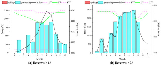
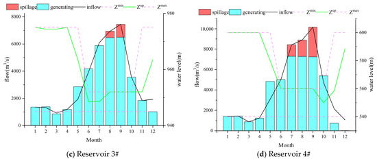
Figure 4. Monthly schedules for inflow scenarios in the year 1973.

The results of the typical hourly load balances for four representative months, selected from each of the four seasons—January, April, July, and October—are shown in Figure 5. The figure corresponds to the load distribution situation of Equation (11). Due to the large number of reservoirs, the legend does not display the power output of each reservoir. It can be seen that SL is 0 in this scenario, indicating that the supply guarantee has been met in these four months. Hydroplants generate as steadily as possible within their capacity, participating in balancing hourly power demands throughout the day. As can be seen, the power export of most hydropower stations is positive and stable each month, indicating that the power demands are reliably met. Only a small portion, or even one hydroplant, has unstable distribution of power output between 12 months. Due to the lowest inflows in January, the power export is also at its minimum despite the lowest daily load demand. In contrast, April and October have the highest load demands, producing the highest stable power exports. Although runoff is abundant in July, power exports are not at their peak because large reservoirs, such as Reservoir 1# and Reservoir 3#, are refilling their water levels during this period.

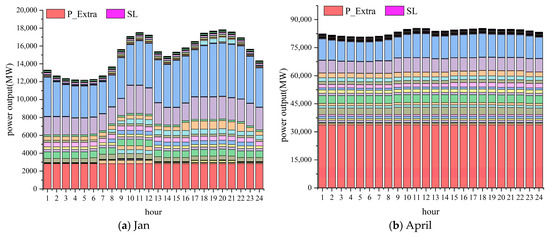
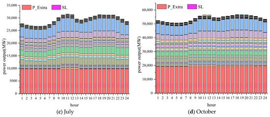
Figure 5. Hourly hydropower schedules on typical days in 1973.

4.3. Power Demand-Met Rate over Storage and Inflow States

Figure 6 shows the hourly power demand-met rate distribution across months in a year. Due to the image being too small, the coordinate axis is blurred. The horizontal axis represents the discrete state of the reservoir capacity, and the vertical axis represents the discrete state of the incoming water from the reservoir. The colors in the picture represent the load demand-med rate (DMR). The small rate is pink, the large one is blue, and there is a white transition in the middle. Please refer to Figure 7 for details. Figure 7 is an enlarged version of the February and August figures in Figure 6, with the corresponding DMR value for each state. The specific state dispersion values can be found in Table 2. The colors in the system state space distribute relatively uniformly during the wet months, indicating that power demand-met rates are less influenced by the system’s storage and inflow conditions. This is particularly noticeable in June and July. When even under historically minimal runoff scenarios, the runoff is still substantial. The entire state space is predominantly covered in blue, representing high demand-met rates. However, during the dry months, from November to May, the color distribution becomes more diverse but shows a trend toward gradual homogenization. In May, this pattern abruptly reverts to the more diversified distribution seen in December at the beginning of the dry season. The results indicate that the impact of runoff conditions on the power demand-met rate diminishes progressively from November to April of the following year, but May, marking the transition between the dry and flood seasons, is a critical month where inflow conditions significantly affect the demand-met rate. As shown in Table 3, the demand-met rate, 98% for example, cannot be met at 41% storage and inflow states during dry months, while only 19% states during wet months. Meeting the power demands for the upcoming year largely depends on the dry months.

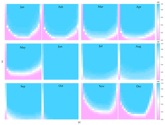
Figure 6. Distribution of demand-met rates over different months.

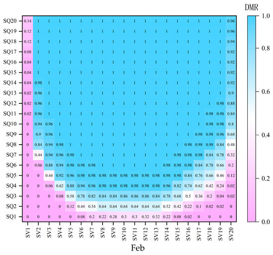
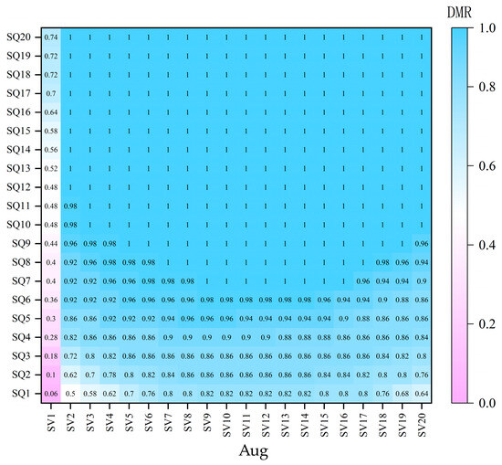
Figure 7. Detailed hourly power demand-met rates in February and August.

Table 3. The rate of the states that cannot meet a demand-met rate of 98%.

Month	Dry Months							Wet Months
	11	12	1	2	3	4	5	6	7	8	9	10
Rate	61%	45%	43%	34%	37%	30%	41%	5%	25%	36%	24%	7%
Average Rate	41%							19%

Figure 7 details the distribution of the demand-met rate across the system state space of storage and inflow conditions for February and August, which are representative months for the dry and flood seasons, respectively. Even in August, during the flood season, when water levels are very low, achieving a satisfactory power demand-met rate for the following year is difficult, even with enough inflow. Compared to August, February shows a lower demand-met rate across a broader range of storage and inflow conditions. In some low-inflow scenarios, both extremely low or high storage levels result in a demand-met rate of zero, meaning it is impossible to meet power demand for the following year. While higher current inflow increases the likelihood of future demand being met, the rate does not consistently rise with increased storage; it first increases and then falls, forming a convex shape. This trend arises because reservoir storage needs to return to its initial state after a one-year operation period to ensure a sustainable supply for the following year. A high initial storage level aids in meeting demand early on but creates difficulties later due to the need to conserve water. Conversely, low initial storage hinders early power demand fulfillment but reduces storage pressure later. Thus, there is an optimal storage level that maximizes the future power demand-met rate.

Figure 8 illustrates monthly storage corridors that can guide operators to achieve specific power demand-met rate levels. When it is difficult to predict or accurately observe the incoming water from a reservoir, the operator often relies on years of operating experience to control the reservoir appropriately to avoid risks. The previous analysis shows that a specific storage range within the storage and inflow state space exists to maximize the power demand-met rate in the coming year, regardless of the inflow conditions. For instance, as illustrated in Figure 7, regardless of the state of inflow, storage levels between V₁₂ and V₁₃ in February and between V₉ and V₁₄ in August can achieve the highest demand-met rates for the year following their respective months under the same inflow state. This does not mean that it is optimal under these storage capacity states, but rather relatively optimal under the same runoff state. Similarly, storage levels between V₁₀ and V₁₁ in February and between V₇ and V₈ and V₁₅ to V₁₇ in August can result in the second-highest demand-met rates for the upcoming year. As shown in Figure 8, drawing the water storage corridors can more easily and intuitively adjust the water storage level of the reservoir to ensure different power demand-met rates. The results show that the most expansive reservoir corridors are found in June and October, indicating that the reservoir has greater flexibility in water level control to achieve the highest power demand-met rate.

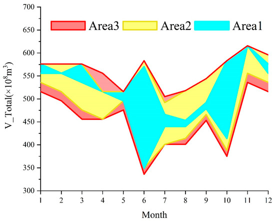
Figure 8. Storage corridor for achieving specific demand-met rate levels.

4.4. Benefits of Hourly Power Balance in Typical Days for Individual Months

Conventionally, monthly hydropower scheduling seeks to sequentially maximize the firm’s hydropower output and total energy production, prioritizing the firm output first, mathematically expressed as

$${\max W}_1·F+W_2\sum _{i=1}^{NR}\sum _{m=0}^{11}{P}_{im}$$

(19)

without hourly power balances (9) and (11) in a typical day for each month, while the generating capacity (10) is enforced on the monthly scale as:

$$P_{im}\le a_{ik}^{\left(2\right)}{\overline{V}}_{im}+b_{ik}^{\left(2\right)}{Q}_{im}^{\mathrm{o}\mathrm{u}\mathrm{t}}+c_{ik}^{\left(2\right)}$$

(20)

Figure 9 compares the optimization results for a historical runoff scenario under a specific storage and inflow system state. It shows that traditional cascade reservoir operations prioritize maximizing guaranteed output, which leads to very stable power generation from October to May during the dry season. However, a stable output is insufficient to ensure the monthly power balance, especially when there is a significant difference in load demand from month to month. As illustrated in Figure 9b, although the traditional scheduling method maintains steady output, it fails to meet electricity demand in May, September, and October, while the model used in this work successfully meets the load demand for each month.

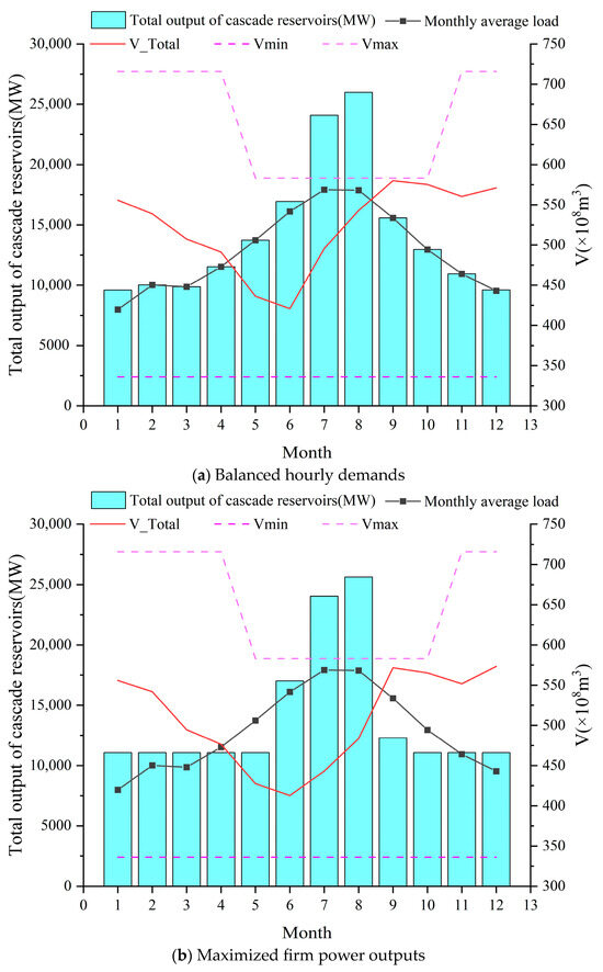
Figure 9. Monthly results with hourly power balances vs. without hourly power balances.

5. Conclusions

This work presents a new procedure to map hourly power demand-met rates over storage and inflow state space of cascaded hydropower reservoirs by simulating multiple years of historical inflow scenarios while considering monthly and hourly power demand variations. Using the overall storage and inflow as the system states simplifies the demand-met distribution map that can serve as an operational rule/chart for cascaded hydropower reservoirs.

The proposed models and procedure were developed as part of an industrial project aimed at assisting operators in making informed decisions to ensure power demand-met reliability.

Applications of present models and procedures for 39 major hydropower reservoirs in China’s hydropower systems are as follows:

• Meeting power demands for the following year depends heavily on proper reservoir management during the dry months. The demand-met rate, 98% for example, cannot be met at 41% storage and inflow states during dry months, while only 19% states during wet months.
• A higher current inflow is more likely to meet the power demands, but an optimal storage level exists to maximize the demand-met rate that is not monotonically increasing to the storage level.
• June and October offer the most flexible storage corridors, giving operators greater control over reservoir levels to achieve the highest demand-met rate.
• Although maintaining stable power output, traditional scheduling methods fail to meet electricity demand in critical months like May, September, and October, while the present model successfully meets load demand in each month.

Future efforts will leverage artificial intelligence to explore and optimize operational rules further, enhancing the adaptability and robustness of the method for real-time applications. In addition to traditional mathematical optimization algorithms, current research also widely applies artificial intelligence (AI) methods to improve the efficiency of power system operation and the effectiveness of energy optimization configuration [30]. From demand and power generation forecasting [31,32] to various energy optimization [33,34] and load management, artificial intelligence plays a crucial role in the construction, planning, and operation of smart grids.

References

- Thaeer Hammid, A.; Awad, O.I.; Sulaiman, M.H.; Gunasekaran, S.S.; Mostafa, S.A.; Manoj Kumar, N.; Khalaf, B.A.; Al-Jawhar, Y.A.; Abdulhasan, R.A. A Review of Optimization Algorithms in Solving Hydro Generation Scheduling Problems. Energies 2020, 13, 2787. [Google Scholar] [CrossRef]
- Xu, C.; Zhu, D.; Guo, W.; Ouyang, S.; Li, L.; Bu, H.; Wang, L.; Zuo, J.; Chen, J. Multi-Objective Ecological Long-Term Operation of Cascade Reservoirs Considering Hydrological Regime Alteration. Water 2024, 16, 1849. [Google Scholar] [CrossRef]
- Beça, P.; Rodrigues, A.C.; Nunes, J.P.; Diogo, P.; Mujtaba, B. Optimizing Reservoir Water Management in a Changing Climate. Water Resour. Manag. 2023, 37, 3423–3437. [Google Scholar] [CrossRef]
- Liu, X.; Yuan, X.; Ma, F.; Xia, J. The increasing risk of energy droughts for hydropower in the Yangtze River basin. J. Hydrol. 2023, 621, 129589. [Google Scholar] [CrossRef]
- Pardis, B.; Matteo, G.; Andrea, C. Partitioning the Impacts of Streamflow and Evaporation Uncertainty on the Operations of Multipurpose Reservoirs in Arid Regions. J. Water Resour. Plan. Manag. 2018, 144, 05018008. [Google Scholar] [CrossRef]
- Bai, T.; Feng, Q.L.; Liu, D.; Ju, C. Reservoir Risk Operation of ‘Domestic-Production-Ecology’ Water Supply Based on Runoff Forecast Uncertainty. Water Resour. Manag. 2024, 38, 3369–3388. [Google Scholar] [CrossRef]
- Cao, C.; He, Y.; Cai, S. Probabilistic runoff forecasting considering stepwise decomposition framework and external factor integration structure. Expert Syst. Appl. 2024, 236, 121350. [Google Scholar] [CrossRef]
- Xu, B.; Sun, Y.; Huang, X.; Zhong, P.; Zhu, F.; Zhang, J.; Wang, X.; Wang, G.; Ma, Y.; Lu, Q.; et al. Scenario-Based Multiobjective Robust Optimization and Decision-Making Framework for Optimal Operation of a Cascade Hydropower System Under Multiple Uncertainties. Water Resour. Res. 2022, 58, e2021WR030965. [Google Scholar] [CrossRef]
- Liu, S.; Xie, Y.; Fang, H.; Huang, Q.; Huang, S.; Wang, J.; Li, Z. Impacts of Inflow Variations on the Long Term Operation of a Multi-Hydropower-Reservoir System and a Strategy for Determining the Adaptable Operation Rule. Water Resour. Manag. 2020, 34, 1649–1671. [Google Scholar] [CrossRef]
- Xu, W.; Zhang, X.; Peng, A.; Liang, Y. Deep Reinforcement Learning for Cascaded Hydropower Reservoirs Considering Inflow Forecasts. Water Resour. Manag. 2020, 34, 3003–3018. [Google Scholar] [CrossRef]
- Salwey, S.; Coxon, G.; Pianosi, F.; Lane, R.; Hutton, C.; Singer, M.B.; McMillan, H.; Freer, J. Developing water supply reservoir oper-ating rules for large-scale hydrological modelling. Hydrol. Earth Syst. Sci. 2024, 28, 4203–4218. [Google Scholar] [CrossRef]
- Ross, L.; Pérez-Santos, I.; Parady, B.; Castro, L.; Valle-Levinson, A.; Schneider, W. Glacial Lake Outburst Flood (GLOF) Events and Water Response in A Patagonian Fjord. Water 2020, 12, 248. [Google Scholar] [CrossRef]
- George, K.Y. Finding Reservoir Operating Rules. J. Hydraul. Div. 1967, 93, 297–322. [Google Scholar] [CrossRef]
- Chen, Y.; Wang, M.; Zhang, Y.; Lu, Y.; Xu, B.; Yu, L. Cascade Hydropower System Operation Considering Ecological Flow Based on Different Multi-Objective Genetic Algorithms. Water Resour. Manag. 2023, 37, 3093–3110. [Google Scholar] [CrossRef]
- Webster, M.; Fisher-Vanden, K.; Kumar, V.; Lammers, R.B.; Perla, J. Integrated hydrological, power system and economic modelling of climate impacts on electricity demand and cost. Nat. Energy 2022, 7, 163–169. [Google Scholar] [CrossRef]
- Wu, C.; Wang, Z.; Yue, P.; Lai, Z.; Wang, Y. Research on Optimal Operation of Cascade Reservoirs under Complex Water-Level Flow Output Constraints. Water 2024, 16, 2963. [Google Scholar] [CrossRef]
- Lai, G.; Luo, J.; Li, Q.; Qiu, L.; Pan, R.; Zeng, X.; Zhang, L.; Yi, F. Modification and validation of the SWAT model based on multi-plant growth mode, a case study of the Meijiang River Basin, China. J. Hydrol. 2020, 585, 124778. [Google Scholar] [CrossRef]
- Zhao, Q.K.; Cai, X.M. Deriving representative reservoir operation rules using a hidden Markov-decision tree model. Adv. Water Resour. 2020, 146, 103753. [Google Scholar] [CrossRef]
- Fu, G.T.; Ni, G.H.; Zhang, C. Recent Advances in Adaptive Catchment Management and Reservoir Operation. Water 2019, 11, 427. [Google Scholar] [CrossRef]
- He, S.K.; Guo, S.L.; Yang, G.; Chen, K.B.; Liu, D.D.; Zhou, Y.L. Optimizing Operation Rules of Cascade Reservoirs for Adapting Climate Change. Water Resour. Manag. 2020, 34, 101–120. [Google Scholar] [CrossRef]
- Gavahi, K.; Mousavi, S.J.; Ponnambalam, K. Adaptive forecast-based real-time optimal reservoir operations: Application to Lake Urmia. J. Hydroinform. 2019, 21, 908–924. [Google Scholar] [CrossRef]
- Wang, J.; Zhao, T.; Zhao, J.; Wang, H.; Lei, X. Improving real-time reservoir operation during flood season by making the most of streamflow forecasts. J. Hydrol. 2021, 595, 126017. [Google Scholar] [CrossRef]
- Li, D.H.; Chen, Y.N.; Lyu, L.Q.; Cai, X.M. Uncovering Historical Reservoir Operation Rules and Patterns: Insights From 452 Large Reservoirs in the Contiguous United States. Water Resources Research 2023, 60, e2023WR036686. [Google Scholar] [CrossRef]
- Liu, S.; Qin, H.; Tang, Z.Y.; Shen, K.Y.; Yang, X.; Zheng, Z.W.; Qu, Y.H.; Jia, Z.W. A novel reservoir dispatching rules extraction framework based on hybrid embedding informer. J. Hydrol. 2024, 644, 132047. [Google Scholar] [CrossRef]
- Li, J.; Zhang, W.; He, B.; Xie, L.; Hao, X.; Mallick, T.; Shanks, K.; Chen, M.; Li, Z. Experimental study on the comprehensive performance of building curtain wall integrated compound parabolic concentrating photovoltaic. Energy 2021, 227, 120507. [Google Scholar] [CrossRef]
- Zhang, W.; Liu, P.; Wang, H.; Chen, J.; Lei, X.; Feng, M. Reservoir adaptive operating rules based on both of historical streamflow and future projections. J. Hydrol. 2017, 553, 691–707. [Google Scholar] [CrossRef]
- Lin, F.; Zhou, Y.; Ning, Z.; Xiong, L.; Chen, H. Exploring a novel reservoir drawdown operation framework for boosting synergies of hydropower generation and drought defense. Sustain. Energy Technol. Assess. 2023, 60, 103562. [Google Scholar] [CrossRef]
- Zhou, F.; Wang, Z.; Chen, D.; Zhang, K. Reservoir Inflow Forecasting in Hydropower Industry: A Generative Flow-Based Approach. IEEE Trans. Ind. Inform. 2023, 19, 1196–1206. [Google Scholar] [CrossRef]
- Zheng, H.; Feng, S.Z.; Chen, C.; Wang, J.W. A new three-triangle based method to linearly concave hydropower output in long-term reservoir operation. Energy 2022, 250, 123784. [Google Scholar] [CrossRef]
- Srinivasan, S.; Kumarasamy, S.; Andreadakis, Z.E.; Lind, P.G. Artificial Intelligence and Mathematical Models of Power Grids Driven by Renewable Energy Sources: A Survey. Energies 2023, 16, 5383. [Google Scholar] [CrossRef]
- Aziz, A.; Mahmood, D.; Qureshi, M.S.; Qureshi, M.B.; Kim, K. AI-based peak power demand forecasting model focusing on economic and climate features. Front. Energy Res. 2024, 12, 1328891. [Google Scholar] [CrossRef]
- Kumar, K.; Prabhakar, P.; Verma, A.; Saroha, S.; Singh, K. Advancements in wind power forecasting: A comprehensive review of artificial intelligence-based approaches. Multimed. Tools Appl. 2024, 1–30. [Google Scholar] [CrossRef]
- Ferdaws, B.N.; Sana, T.; Chokri, B.S.; Mohamed, A.M.; Mehdi, T. Decision-making solutions based artificial intelligence and hybrid software for optimal sizing and energy management in a smart grid system. Concurr. Eng. 2024, 32, 3–19. [Google Scholar]
- Feng, Z.K.; Niu, W.J.; Zhang, T.H.; Wang, W.C.; Yang, T. Deriving hydropower reservoir operation policy using data-driven artificial intelligence model based on pattern recognition and metaheuristic optimizer. J. Hydrol. 2023, 624, 129916. [Google Scholar] [CrossRef]
Disclaimer/Publisher’s Note: The statements, opinions and data contained in all publications are solely those of the individual author(s) and contributor(s) and not of MDPI and/or the editor(s). MDPI and/or the editor(s) disclaim responsibility for any injury to people or property resulting from any ideas, methods, instructions or products referred to in the content. |
© 2024 by the authors. Licensee MDPI, Basel, Switzerland. This article is an open access article distributed under the terms and conditions of the Creative Commons Attribution (CC BY) license (https://creativecommons.org/licenses/by/4.0/).