Indian Summer Monsoon and El Niño Southern Oscillation in CMIP5 Models: A Few Areas of Agreement and Disagreement

Abstract

Using the CMIP5 model outputs, a few characteristics of Indian Summer Monsoon (ISM) rainfall and Niño 3.4 temperature are analysed during June–July–August–September (JJAS). Focusing on specified regions around central-northeast India, some general characteristic features of ISM precipitation are studied, which are shown to be varying among models. The trend of decreasing rainfall in that region as noticed in observations suggests an inconsistency among models. The ENSO also shows variation, and its phasing indicates disagreement. Unlike other models, FGOALS-g2 is identified as not suggesting any trend in Niño 3.4 temperature and needs attention for model evaluation purposes. ISM and ENSO correlation in either historical or the RCP 8.5 scenario confirm a negative signature, agreeing with the usual ISM, ENSO connection. Precipitation over the globe shows a rising trend in an ensemble of CMIP5 model outputs for the RCP 8.5 scenario, though no consensus is reached for the Indian region. Precipitation time series around the Indian subcontinent vary widely among models. Analyses with various future scenarios indicate that the Indian subcontinent shows much larger uncertainty, in terms of precipitation, compared to that from the whole world. This study identifies a few areas where CMIP5 models are in agreement or disagreement with each other. Such an analysis could be useful for understanding various processes in CMIP5 models that involve ISM precipitation and can lead to improving the representation of processes in models.

1. Introduction

Indian Summer Monsoon (ISM) has enormous impacts not only on the Indian economy, but also on the global economy. It provides the major share of the total annual rainfall of the country, and being one of the most populated countries in the world, its variations influence the global economy. Moreover, the ISM system also has an important contribution to the atmospheric circulation, by dominating the northern summer Hadley circulation [1].

The boreal summer (June–July–August–September (JJAS)) climatological precipitation has a widespread maximum over Central Northeast (CNE) India, which includes the Indo-Gangetic Plain. The ISM represents a large-scale heat source around the CNE India, which could be related to both the regional Hadley and Walker cell, following the linear theory [2]. Hence, additional attention was given to that region. A number of observational works has investigated the trend of monsoon rainfall over India during the climate change period of the last half of the 20th century [3,4]. Considering a region (76°–87° E, 20°–28° N) around the CNE India, a study [5] detected a decreasing trend for ISM precipitation. They analysed the period of 1940–2005 and used the NOAA GFDL CM 3 model for all forcing (natural and anthropogenic) conditions. The Climate Research Unit (CRU) observational data also showed a marked reduction from the 1950s to the end of the 20th century (statistically significant at the 95% confidence level). That observation is compared with the model output in that study [5]. The results from CRU are also broadly consistent with previous observational studies [4,6,7]. Another study [8], using a slightly different region around the similar location of central-northern India (74.5° E–86.5° E and 16.5°N–26.5° N), also found a decreasing trend of ISM rainfall. Though the observational results indicated a drying trend, it is interesting to explore using various model outputs whether there is any consensus among model results. The initial focus here is on an analysis region of a location and size similar to that used by the earlier mentioned study [5]. Later, it also included a region around CNE as considered by [8]. Those two regions are marked by CI and CII respectively in Figure 1.

A recent study [9] discussed how the response of precipitation changes varies regionally with respect to the global warming scenario. For the tropical ocean, two viewpoints exist. One predicts ‘wet-gets-wetter’, which means more rainfall in precipitation-prone regions [10,11]. The other suggests ‘warmer-gets-wetter’, meaning increased precipitation would occur with a rise in sea surface temperature. Further analyses [12,13,14], however, suggested that the two mechanisms are complementary and not contradictory. Those mentioned that the variability of the annual mean precipitation over the tropical ocean follows the ‘warmer-gets-wetter’ mechanism, but the seasonal mean precipitation suggests the ‘wet-gets-wetter’ rule. The precipitation in the high to mid-latitudes has enhanced by 0.5–1% per decade, which is consistent. There is an exception though over East Asia [15], and the reason for such a deviation in East Asia is still poorly understood [16,17]. The drying trend around the CNE region of India is consistent with such a deviation.

Studies have identified clear connections between the ISM and the El Niño Southern Oscillation (ENSO) [18]. Such associations were also recently discussed [19], which put emphasis on the climate change period of the last half of 20th Century. It also discussed the role of the North Atlantic Oscillation (NAO) and the Indian Ocean Dipole (IOD). A research [20] analysed ISM-ENSO teleconnection during the latter half of the last century using the reanalysis product. They proposed a route, whereby the ISM could have a remote influence via the modification of Eurasian temperature. In examining ISM-ENSO connections, studies even identified modulating roles of atmosphere-ocean coupling systems originated in the Northern Hemisphere (via (Pacific Decadal Oscillation) PDO [21] and the North Atlantic [22]). On the other hand, using wavelet techniques on observational data, [23] suggested an inter-decadal variation in the monsoon-ENSO behaviour. They showed that it is true, irrespective of the analysis method and different datasets. The ISM is such a complicated system that understanding and predicting its varied behaviour is always a challenge. Noticeable improvements in forecasting are realized through the inclusion of more detailed physics of the climate and higher resolution in models. A major step forward is the incorporation of coupled ocean-atmosphere models, those including air-sea interaction.

However, most of the current generation climate models are still not capable of simulating realistic ENSOs [24,25]. The overall skill of ENSO prediction in retrospective forecasts made with ten different coupled GCMs was also investigated [26]. It analysed seasonal output from the APCC/CliPAS (Asian-Pacific Economic Cooperation Climate Center/Climate Prediction and its Application to Society) and DEMETER (Development of a European Multi-model Ensemble system for seasonal to inTER-annual prediction) projects during the common 22 years from 1980 to 2001. They indicated that the overall prediction skill is in need of improvement. Recent modelling studies [26,27] have also confirmed this. Given the crucial role played by the Pacific in the global climate, advancement of our knowledge relating to the ENSO is obviously important.

A recent collective initiative among different modelling communities around the world conducted similar experiments that comprised the Coupled Model Inter-comparison Project, Phase 5 (CMIP5) (link: http://cmip-pcmdi.llnl.gov/cmip5/experiment_design.html). The details are all described clearly [28]. Changes in ENSO variability during 2050–2100 are studied using CMIP3 (third phase of Coupled Model Inter-comparison Project) experiments [25]. In terms of the amplitude of ENSO, they showed that models are still unable to reach consensus for predictions in the future. However, the coupled CMIP5 models are more capable of simulating ENSO-like interannual variability in the central and eastern equatorial Pacific [29]. Compared to the CMIP3 group of models, more CMIP5 models show a realistic range of ENSO frequencies in the band of 2–7 years in the equatorial Pacific. Nearly half of the CMIP5 models show Sea Surface Temperature (SST) anomalies peaking from November–January, as seen in observations. It is of considerable importance to determine how ENSO responds under rising amounts of greenhouse gases [30]. Numerous studies also discussed the evolution of ENSO in the Representative Concentration Pathway (RCP) scenario runs [31,32], though uniform consensus is yet to be reached.

Using CMIP3 experiments, a study [33] examined ISM precipitation averaged over land regions (60–90° E, 7–27° N). They also elaborately discussed various issues as to why models fail to match observations and indicated that advanced understanding and model improvements are essential for improving the skill of ISM prediction. In terms of mechanisms relating to disagreement among model results and observations, various studies addressed this from different angles (those include sea-surface temperatures in the Indo-Pacific [34]; circulation-based changes [34]; and aerosol-based changes [5]). Using the model, it was noted [35] that for observed fluctuations in the ENSO-ISM correlation, sampling variability can also be a responsible factor.

A recent work [36] discussed ISM precipitation in detail and compared CMIP3 with CMIP5 models. It elaborately discussed its linkage with ENSO. The performance of CMIP5 is shown to be improved. Relating to the ENSO-ISM teleconnection, recent research [37,38] also considered various CMIP5 model outputs. In those studies, they elaborately discussed the teleconnection focusing on two different types of ENSO: Eastern Pacific (EP)-type ENSO (and often known as Canonical ENSO) and Central Pacific (CP)-type ENSO (often known as Modoki ENSO). This is because various studies suggested that there are differences in global and local influences between ENSO Modoki and Canonical ENSO ([39], among others). Focusing on ISM, it was indicated [38] that more than 80% of the CMIP5 models capture ENSO-ISM regional teleconnections around the CNE region, irrespective of EP or CP ENSO category.

A few of the principal aims of the CMIP5 project are assessing the mechanisms responsible for model differences and determining why similarly forced models are producing a range of responses, among others [28]. The proper phasing and teleconnections of ISM-ENSO on various time scales could also be an important aspect to explore. The current study tries to explore those areas relating to ISM precipitation and Niño temperature, using CMIP5 model outputs.

The structure of this study is as follows. Section 2 discusses the methodology and data. In the Results section, first, the temporal and spatial pattern of ISM around regions in CNE using CMIP5 models (Section 3.1) is the focus. This is followed by some characteristics of Niño 3.4 in models (Section 3.2). Later, ISM and Niño3.4 correlation (Section 3.3), while Section 3.4 compares ISM with global precipitation in future scenarios. Conclusions are presented in Section 4. Overall, this study identifies a few areas where the CMIP5 models show consistencies/disagreements with observations. It also presents an overview of future scenarios.

2. Methodology and Data

Various common statistical techniques are used; those include time series analysis, applying the eleven-year running average, the spatial pattern of trend using the method of mean differences, etc. Regarding time series analysis, the variation of a parameter is initially calculated with respect to its average over a reference period. For ISM, an eleven-year running average method is applied to have a clearer overview relating to the longer term trend. Such smoothing is also applied in analysing the ISM trend [33]. To examine the spatial pattern of trends, mean values of precipitation during the period of consideration are subtracted from those from the average of a reference period. Precipitation data for various models during the historical and RCP scenarios were collected from the CMIP5 website (http://cmip-pcmdi.Llnl.gov/cmip5/experiment_design.html). Details of forcing and the model setup are all well documented [28]. RCP 8.5 indicates Representative Concentration Pathway 8.5, and this means that it leads to an approximate radiative forcing of 8.5 W/m². Different RCP scenarios are also considered (e.g., RCP 2.6, RCP 4.5 and RCP 6.0). Niño 3.4 temperature for the models is also obtained from that site.

Various models are used, and those include the coupled version (CMIP5), as well as an atmospheric version (AMIP5) (Atmospheric Model Intercomparison Project phase 5). Models are also separated as High top (H) or Low top (L), as shown in

Table 1. Various modelling centres, with the name of the model types, CMIP5 and AMIP5. Models are separated as Low top (L) or High top (H).

Model Centre	Model Type		Model ID (Chosen)	High Top (H)/Low Top (L)
	CMIP5	AMIP5
CSIRO-BOM, Australia	ACCESS1.0	ACCESS1.0	A	L
	ACCESS1.3	ACCESS1.3	B	L
BCC, China	BCC-CSM1.1	BCC-CSM1.1	C	L
	BCC-CSM1.1(m)	BCC-CSM1.1(m)	D	L
GCESS, China	BNU-ESM	BNU-ESM	E	L
CCCMA, Canada	CanESM2	CanAM4	F	L
NCAR, USA	CCSM4	CCSM4	G	L
CMCC, Italy	CMCC-CM	CMCC-CM	H	L
CNRM-CERFACS, France	CNRM-CM5	CNRM-CM5	I	L
CSIRO-QCCCE, Australia	CSIRO-Mk3.6.0	CSIRO-Mk3.6.0	J	L
LASG-CESS, China	FGOALS-g2	FGOALS-g2	K	L
LASG-IAP, China	FGOALS-s2	FGOALS-s2	L	L
INM, Russia	INM-CM4	INM-CM4	M	L
MIROC, Japan	MIROC5	MIROC5	N	L
NCC, Norway	NorESM1-M	NorESM1-M	O	L
NOAA-GFDL, USA	GFDL-CM3	GFDL-CM3	P	H
MOHC, England	HadGEM2-CC	HadGEM2-A	Q	H
NASA-GISS, USA	GISS-E2-R	GISS-E2-R	R	H
IPSL, France	IPSL-CM5A-LR	IPSL-CM5A-LR	S	H
	IPSL-CM5A-MR	IPSL-CM5A-MR	T	H
MPI-M, Germany	MPI-ESM-LR	MPI-ESM-LR	U	H
	MPI-ESM-MR	MPI-ESM-MR	V	H
MRI, Japan	MRI-CGM3	MRI-CGCM3	W	H

. High top models are those that have upper lids up to the stratopause (1 hPa) and/or few model layers in the stratosphere. However, in this study, the main results did not change using either the AMIP or CMIP version, or choosing the high top or low top one. Hence, the results for only the CMIP5 models are presented here.

3. Results

3.1. Spatial and Temporal Pattern of ISM Rainfall in the CNE Region

Following the previous work [5], this paper initially attempts to investigate the spatial and temporal pattern of ISM precipitation in the same region (CI, Figure 1) during a similar period (1940–2005) using various CMIP5 model outputs. Earlier, it was also discussed why the CNE region would show different teleconnection mechanisms [2]. Figure 2 focuses on the spatial pattern, while Figure 3 and Figure 4 focus on the temporal variation.

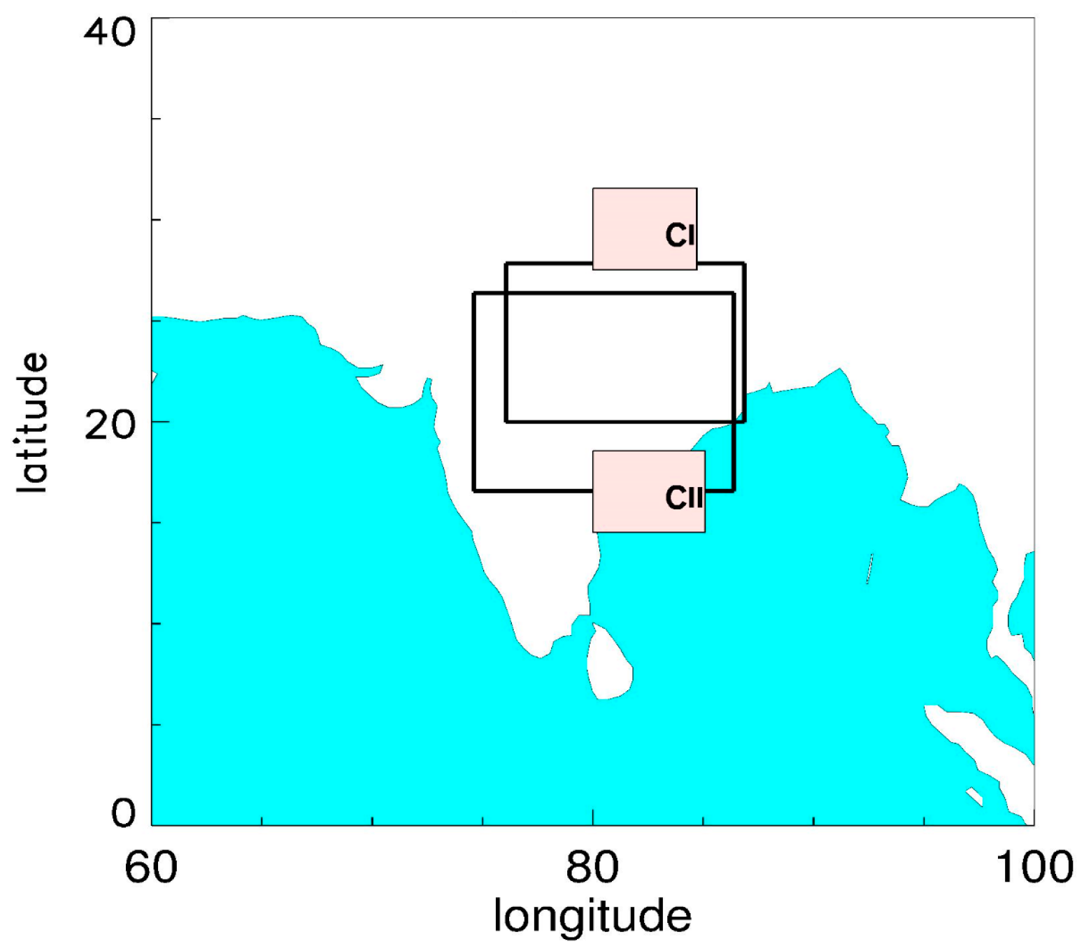
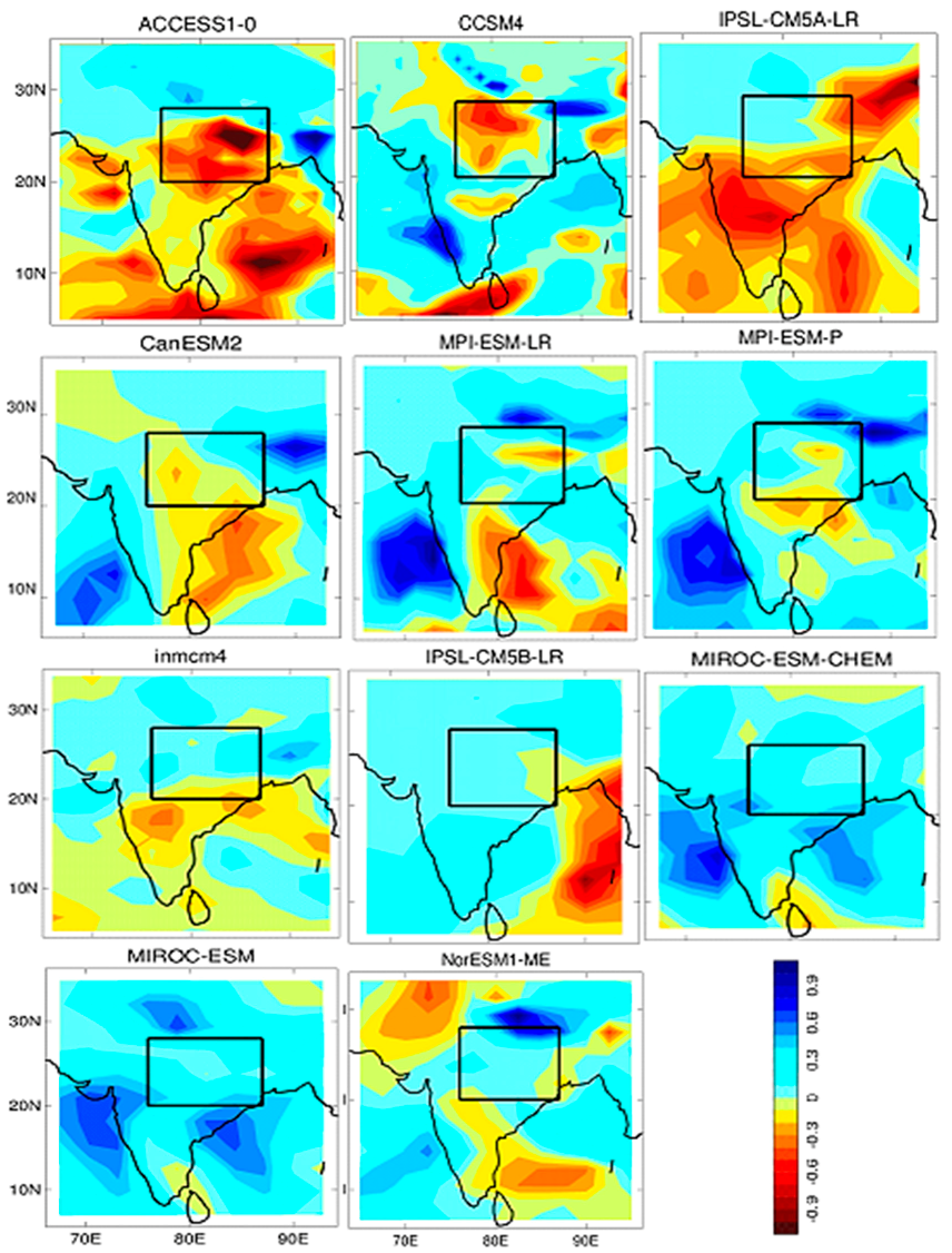
3.1.1. Spatial Patterns in the CI Region

Figure 2 shows the precipitation anomaly using various CMIP5 models. To investigate the nature of variation in the spatial pattern, mean values of precipitation during the period of 1940–2005 are subtracted from those of the average for the period of 1986–2005 of the respective models. Such anomaly calculations can indicate whether there is a rising or decreasing trend during a later period. For example, if the calculated anomaly indicates a positive result, this suggests that there is a decrease in rainfall during the later period (1986–2005) as the anomaly calculated relative to that period. The region CI in CNE India is marked by a dark black rectangle. The red colour in that region suggests a rise in the precipitation during the later period (as an anomaly with respect to that period). In other words, to compare with [5], it can be said that there is a rising trend. From Figure 2, it is clear that unlike their results, we do not find a clear consensus among various CMIP5 models as presented here. Figure 2 shows models dominated by a rising trend in Row 1, to models dominated by a decreasing trend in the last row, with models without much indications of a trend in between. Significant regions are not marked, as our main objective here is to show the diverse behaviour among models rather than the amplitude. Results from a few models are presented, and the rest of the models also suggest similar results. Analyses were repeated for the CII region, as well, and the main findings did not change and hence are not shown. It is noteworthy that this study is not restricted to a few particular models, as the main purpose is to present the diverse behaviour among models.

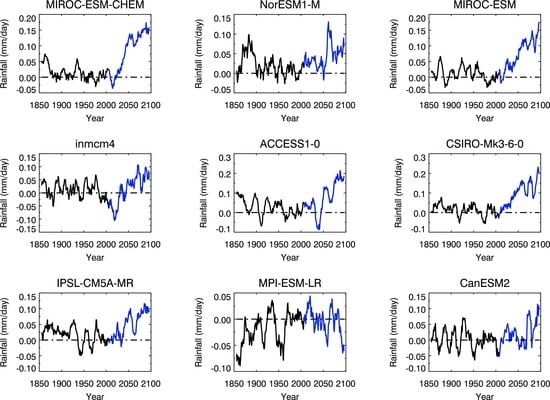
3.1.2. Temporal Patterns in the CI Region

Figure 3 shows the temporal variation of precipitation in the same region. It is an anomaly time series plot during the period of 1940–2005, the anomaly having been calculated with respect to the average of the overall period of 1940–2005. The anomaly here is calculated over 1940–2005 because points will be equally distributed around zero lines, and this helps to identify clear trends, if any. An eleven-year running average method is applied to that time series, to have a clearer overview relating to the longer term trend. Figure 3 clearly indicates that there is no common consensus among models and suggests a decreasing trend for the models INM-CM4, ACCESS1-0, MIROC-ESM, NorESM1-M, while there is an increasing trend for IPSL-CM5B-LR, MPI-ESM-LR, MPI-ESM-P, IPSL-CM5A-MR. This study is in line with a previous study [33], despite the different time period, different groups of models (CMIP5 instead of CMIP3) and different regions of analysis (CI region, with a different teleconnection mechanism). This strengthens the finding of [40], who discussed that the fact of disagreement should be considered with care while interpreting ISM-ENSO diagnostics and the response of ISM in a global warming scenario.

In Figure 2 and Figure 3, the focus is on the time period of 1940–2005, as those compared results of [5]. In Figure 4, however, the overall historical period (1850–2005) is also considered to have a general overview. To have a clearer idea relating to a future scenario in the CI region, precipitation in the RCP8.5 scenario is also plotted. The anomaly period is considered as the period of 1985–2005. In this plot, the historical period is represented by black, whereas the RCP8.5 scenario up to 2100 is shown by blue. Eleven-year smoothing is applied to the whole time series. It is clear that though there is a rising trend in precipitation in the CI region among most of the models in the future scenario that follows the ‘wetter-gets-wetter’ and ‘warmer-gets-wetter’ mechanisms [10,11,12,13], there are still some models, e.g., MPI-ESM-LR, that show a decreasing trend.

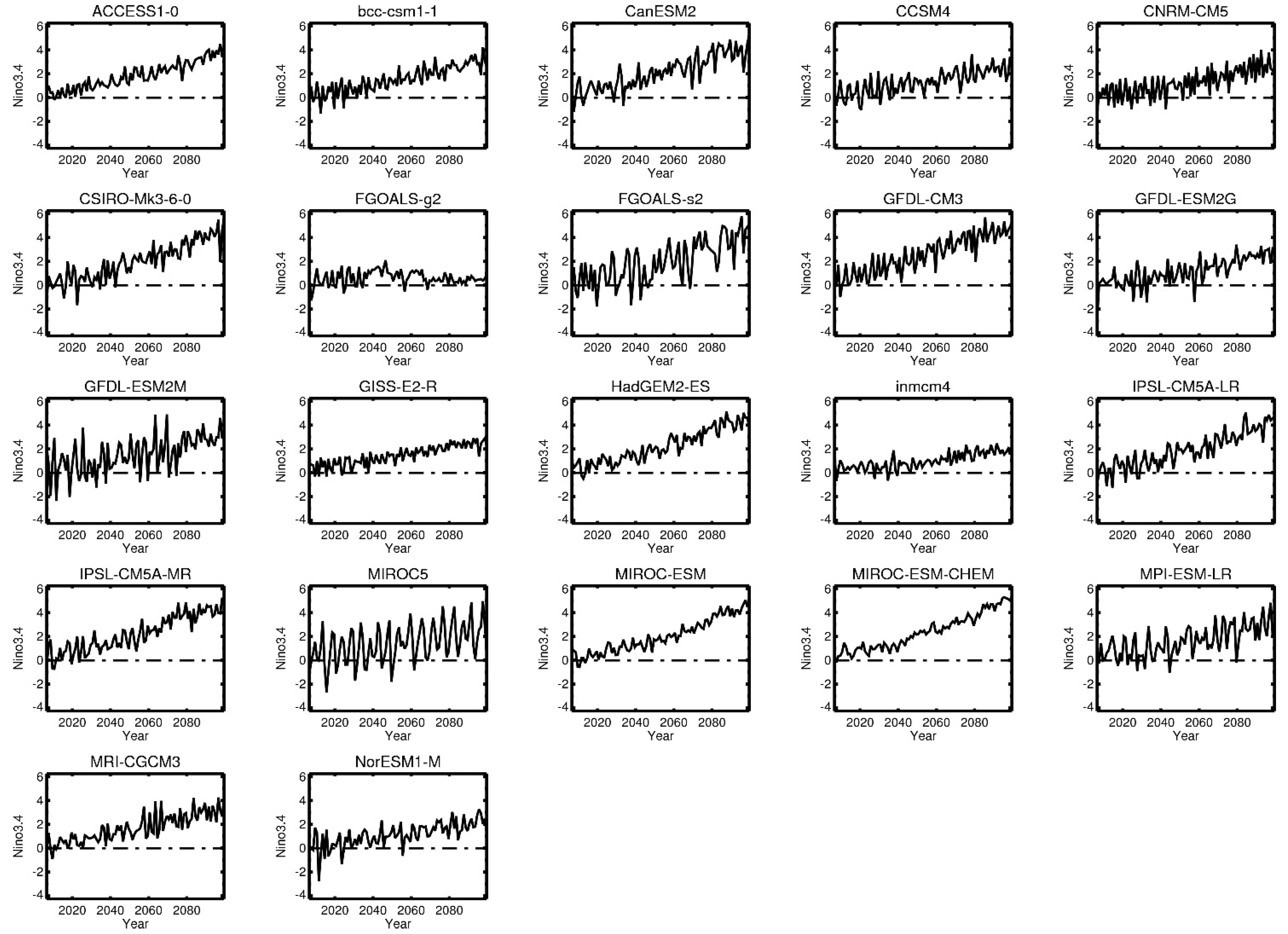
3.2. Niño 3.4 in the RCP Scenario

Figure 5 shows the time series of sea surface temperature in the Niño 3.4 region for the RCP 8.5 scenario. An anomaly is calculated relative to the period (1985–2005). The Y-axis range is kept constant to show the difference in variability and the trend among models.

It is apparent from Figure 5 that for some models, the Niño 3.4 temperature is highly variable when compared to the others. For example, model MIROC5 indicates a highly variable Niño temperature. Other models that also suggest a similar result are GFDL-ESM2M and FGOALS-s2. Some models in that figure can be identified showing the least variable Niño temperature for, e.g., inmcm4, MIROC-ESM and MIROC-ESM-CHEM. The variability suggests a similar result during the historical period of the respective models (hence not shown). Years of the peak and trough of Niño variability differ among the models during the historical and the RCP scenario. This indicates that the coupled atmosphere-ocean model groups need to work on improving the capability of simulating the phasing of ENSO phenomena. The ENSO, being the most important tropospheric variability that influences almost every part of the globe through teleconnection, thus needs its representation in models to be improved. It could be an important step to understanding and predicting global climate features at the sub-seasonal scale for those who use the models.

In terms of the trend in Niño temperature for the RCP scenario, model results also vary (Figure 5); some models show a small trend, e.g., inmcm4, NorESM1-M (see the Y-axis), while some suggest a larger trend, e.g., GFDL-CM3, MIROC-ESM, MIROC-ESM-CHEM. Despite the varied degree of the trends seen (small trend or larger trend), all models show a rising trend in the RCP scenario, with one exception for the model FGOALS-g2. This particular model fails to indicate anything about the Niño trend and thus needs to be investigated further for such a discrepancy. These issues might be addressed to that particular modelling group responsible for the model evaluation task.

3.3. Correlation between ISM and Niño 3.4 in the Historical and RCP Scenario

Table 2. ISM and ENSO correlation using various CMIP5 models (in the whole Indian subcontinent and the two regions, CI and CII) during the historical and RCP 8.5 scenario, after removing the trend.

Model ID	CMIP5 Model Name	Correlation: Rainfall vs. Niño 3.4
		Whole India		Region (CI)		Region (CII)
		Historical	RCP	Historical	RCP	Historical	RCP
A	ACCESS1.0	−0.33	−0.19	−0.13	−0.14	−0.14	−0.20
B	ACCESS1.3	−0.42	−0.24	−0.29	−0.13	−0.28	−0.07
C	BCC-CSM1.1	−0.14	−0.15	−0.14	−0.14	−0.14	−0.14
D	BCC-CSM1.1(m)	−0.42	−0.03	−0.34	−0.17	−0.43	−0.22
E	BNU-ESM	−0.51	−0.64	−0.33	−0.18	−0.29	−0.04
F	CanESM2	−0.52	−0.64	−0.33	−0.34	−0.33	−0.35
G	CCSM4	−0.71	−0.57	−0.42	−0.14	−0.47	−0.36
H	CMCC-CM	−0.18	−0.29	−0.33	−0.51	−0.35	−0.55
I	CNRM-CM5	−0.40	−0.36	−0.37	−0.37	−0.40	−0.33
J	CSIRO-Mk3.6.0	−0.24	−0.31	−0.28	−0.40	−0.28	−0.37
K	FGOALS-g2	−0.31	−0.51	−0.30	−0.48	−0.26	−0.48
L	FGOALS-s2	−0.37	−0.51	−0.29	−0.44	−0.18	−0.33
M	INM-CM4	−0.45	−0.40	−0.38	−0.28	−0.33	−0.22
N	MIROC5	−0.64	−0.74	−0.35	−0.39	−0.30	−0.48
O	NorESM1-M	−0.79	−0.70	−0.51	−0.47	−0.59	−0.52
P	GFDL-CM3	−0.49	−0.27	−0.25	−0.22	−0.26	−0.20
Q	HadGEM2-CC	−0.27	−0.26	−0.38	−0.32	−0.36	−0.35
R	GISS-E2-R	−0.26	−0.56	−0.07	−0.26	−0.06	−0.25
S	IPSL-CM5A-LR	−0.61	−0.61	−0.54	−0.57	−0.62	−0.61
T	IPSL-CM5A-MR	−0.69	−0.56	−0.64	−0.53	−0.67	−0.54
U	MPI-ESM-LR	−0.36	−0.47	−0.37	−0.51	−0.23	−0.52
V	MPI-ESM-MR	−0.17	−0.36	−0.27	−0.49	−0.15	−0.37
W	MRI-CGM3	−0.10	0.11	−0.51	−0.47	−0.24	−0.22

is formulated to investigate the correlation between ISM rainfall and Niño 3.4 temperature. It is calculated during the historical, as well as the RCP 8.5 scenario. For rainfall, the region of the whole Indian subcontinent is considered separately alongside the two regions, CI and CII. The trend is removed from both time series before doing calculations. The negative signature in the correlation value is clearly noticed for all cases irrespective of the historical or RCP scenario. Thus, the CMIP5 models capture the usual ISM and Niño temperature behaviour well, suggesting less rainfall during the El Niño phase and more during La Niña [18].

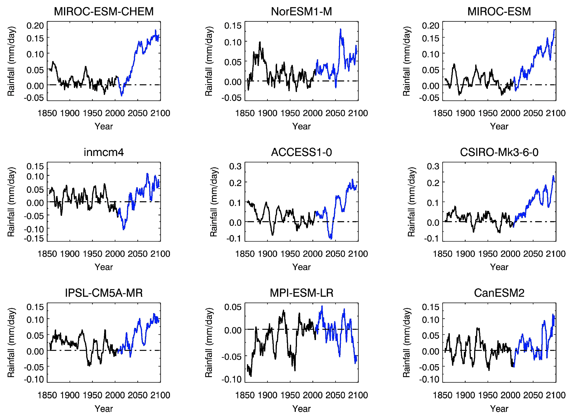
3.4. Precipitation in RCP Scenarios

The precipitation in the high to mid-latitudes has enhanced by 0.5–1% per decade, which is consistent with the ‘wet-gets-wetter’ [10,11] and ‘warmer-gets-wetter’ mechanisms [12,13] and was discussed earlier. However, a drying trend around the CNE region of India suggests a deviation. The following analysis presents a comparison between precipitations around India versus global precipitation on a longer term basis.

Models are considered as a major viable tool to predict future scenarios. Here, some simulations for the future are analysed for precipitation and presented in Figure 6. Precipitation time series in the land region in the RCP 8.5 scenario are calculated for the period 2005–2100 with respect to the average of 1985–2005. Figure 6a shows this for the whole globe and land region, whereas Figure 6b only for the Indian subcontinent. For the globe (Figure 6a), there is a clear rising trend noticed. The spread among models increases with time, showing the maximum spread at around the year 2100. However, in the case of the Indian subcontinent (Figure 6b), it is not possible to identify any clear trend pattern among the model results. Moreover, throughout the period, there is a larger spread. This indicates that CMIP5 models are unable to clearly predict the temporal evolution of ISM rainfall and that the models vary to a greater degree among each other.

The rise in global precipitation for models in a global warming situation (Figure 6a) is in agreement with the popular theory of thermodynamic scaling proposed by [11], and it supports the theory of the ‘warmer-gets-wetter’ [12,13] and ‘wet gets wetter’ [10] mechanisms. However, why such a relationship is not true around the India subcontinent (Figure 6b) needs to be investigated. During the last half of the 20th Century, the so-called global warming period, the observation suggests a decreasing trend in precipitation around India [3,4], contradicting the proposed hypothesis. Such a deviation around East Asia is also noted in other studies [15], though the cause is yet to be understood [16,17].

This study further explores the rainfall pattern over the globe for a land region (Figure 7a) and the CI region (Figure 7b) in various RCP scenarios (RCP 8.5, RCP 6.0, RCP 4.5 and RCP 2.6). The plots for all of India and the CII region show similarities to the CI region and, hence, are not shown. The main point to note is the difference in the spread between Figure 7a,b, as seen through the scales of the Y-axis. The range of uncertainty in the lower plot is very large compared to the top one. Both plots show a general rise in precipitation in various future scenario conditions, which agrees with the mechanisms proposed earlier [10,11,12,13]. The bottom plot, however, does not indicate any decrease in precipitation, as shown by observation and [5].

There was an explanation for why the rainfall pattern around India, especially the CNE region, changed during the later decades of the last century [5]. The direction of the anomalous change in circulation, both the Hadley and Walker circulation and their relative strength around the Indian subcontinent under the climate change scenario, needs additional attention. Such an anomalous change in both the zonal and meridional circulation can oppose/reinforce the regional climatological overturning. Furthermore, the changes in the location of ascent and descent are likely the causes of the changing regional ISM rainfall pattern, which further need to be explored to advance our understanding of future ISM predictions.

4. Conclusions

Some general features of ISM precipitation were explored. It was found that the trend pattern around the CNE region of India varies from model to model. The trend of decreasing rainfall around CNE India, as detected in the observations, though noticed in some models, is not true for every case. Various ENSO features also differ in the models; those include variability, trend, phasing, etc. This is also true for historical, as well as RCP scenarios. Interestingly, unlike other models, the model FGOALS-g2 does not show any trend in Niño 3.4 temperature for either the historical or RCP 8.5 scenario. This observation could be useful for model evaluation purposes. ISM and ENSO correlation was also studied in the historical and RCP 8.5 scenarios, for all of India, as well as two specific regions of India (CI and CII). This suggests a negative correlation for almost all models. Precipitation during JJAS in land regions of the globe shows a clear rising trend in all CMIP5 model outputs for the RCP 8.5 scenarios, but the same for the Indian subcontinent fails to indicate anything clearly. The various future scenarios suggest a much larger uncertainty for ISM rainfall (CI region) in comparison to global precipitation, and the model ensemble does not indicate any decrease in precipitation for India.

In this study, we not only identified some areas where the CMIP5 models show disagreements, but also discussed some aspects where most models agree. Such analyses could be beneficial for improving models and gaining a better understanding of the process representation in models. Additional observations relating to FGOALS-g2 could be used for model evaluation purposes. Finally, this study also provides an indication for the longer term trend of future precipitation.

References

1. Trenberth, K.E.; Hurrell, J.W.; Stepaniak, D.P. The Asian Monsoon; Wang, B., Ed.; Springer: Berlin/Heidelberg, Germany; New York, NY, USA, 2006; pp. 417–457. [Google Scholar]
2. Gill, A.E. Some simple solutions for heat-induced tropical circulation. Q. J. R. Meteorol. Soc. 1980, 106, 447–462. [Google Scholar] [CrossRef]
3. Ramanathan, V.; Chung, C.; Kim, D.; Bettge, T.; Buja, L.; Kiehl, J.T.; Wild, M. Atmospheric brown clouds: Impacts on South Asian climate and hydrological cycle. Proc. Natl. Acad. Sci. USA 2005, 102, 5326–5333. [Google Scholar] [CrossRef] [PubMed]
4. Chung, C.E.; Ramanathan, V. Weakening of the North Indian SST gradients and the monsoon rainfall in India and the Sahel. J. Clim. 2006, 19, 2036–2045. [Google Scholar] [CrossRef]
5. Bollasina, M.A.; Ming, Y.; Ramaswamy, V. Anthropogenic Aerosols and the Weakening of the South Asian Summer Monsoon. Science 2011, 334, 502–505. [Google Scholar] [CrossRef] [PubMed]
6. Lau, K.M.; Kim, K.M. Fingerprinting the impacts of aerosols on longterm trends of the Indian summer monsoon regional rainfall. Geophys. Res. Lett. 2010, 37, L16705. [Google Scholar] [CrossRef]
7. Zhang, L.; Zhou, T. An assessment of monsoon precipitation changes during 1901–2001. Clim. Dyn. 2011, 37, 279–296. [Google Scholar] [CrossRef]
8. Goswami, B.N.; Venugopal, V.; Sengupta, D.; Madhusoodanan, M.S.; Xavier, P.K. Increasing Trend of Extreme Rain Events Over India in a Warming Environment. Science 2006, 314, 1442–1445. [Google Scholar] [CrossRef] [PubMed]
9. Deng, Y.Y.; Gao, T.; Gao, H.W.; Yao, X.H.; Xie, L. Regional precipitation variability in East Asia related to climate and environmental factors during 1979–2012. Sci. Rep. 2014, 4, 5693. [Google Scholar] [CrossRef] [PubMed]
10. Chou, C.; Neelin, J.; Chen, C.; Tu, J. Evaluating the “rich-get-richer” mechanism in tropical precipitation change under global warming. J. Clim. 2009, 22, 1982–2005. [Google Scholar] [CrossRef]
11. Held, I.M.; Soden, B.J. Robust responses of the hydrological cycle to global warming. J. Clim. 2006, 19, 5686. [Google Scholar] [CrossRef]
12. John, O.; Allan, R.P.; Soden, J. How robust are observed and simulated precipitation responses to tropical ocean warming? Geophys. Res. Lett. 2009, 36, L14702. [Google Scholar] [CrossRef]
13. Xie, S.P.; Deser, C.; Vecchi, G.A.; Ma, J.; Teng, H.; Wittenberg, A.T. Global Warming Pattern Formation: Sea Surface Temperature and Rainfall. J. Clim. 2010, 23, 966–986. [Google Scholar] [CrossRef]
14. Huang, P.; Xie, S.P.; Hu, K.; Huang, G.; Huang, R. Patterns of the seasonal response of tropical rainfall to global warming. Nat. Geosci. 2013, 6, 357–361. [Google Scholar] [CrossRef]
15. Folland, C.K.; Karl, T.R.; Christy, J.R.; Clarke, R.A.; Gruza, G.V.; Jouzel, J.; Mann, M.E.; Oerlemans, J.; Salinger, M.J.; Wang, S.W. Climate Change 2001: The Scientific Basis: Contribution Of Working Group I to the IPCC Third Assessment Report; Cambridge University Press: Cambridge, UK, 2001; pp. 99–181. [Google Scholar]
16. Ramanathan, V.; Crutzen, P.J.; Kiehl, J.T.; Rosenfeld, D. Aerosols, climate and the hydrological cycle. Science 2001, 294, 2119–2124. [Google Scholar] [CrossRef] [PubMed]
17. Zhang, X.; Zwiers, F.W.; Hegerl, G.C.; Lambert, F.H.; Gillett, N.P.; Solomon, S.; Stott, P.A.; Nozawa, T. Detection of human influence on twentieth-century precipitation trends. Nature 2007, 448, 461–465. [Google Scholar] [CrossRef] [PubMed]
18. Maity, R.; Kumar, D.N. Bayesian dynamic modelling for monthly Indian summer monsoon rainfall using El Niño–Southern Oscillation (ENSO) and Equatorial Indian Ocean Oscillation (EQUINOO). J. Geophys. Res. 2006, 111, D07104. [Google Scholar] [CrossRef]
19. Roy, I.; Collins, M. On identifying the role of Sun and the El Niño Southern Oscillation on Indian Summer Monsoon Rainfall. Atmos. Sci. Lett. 2015, 16, 162–169. [Google Scholar] [CrossRef] [Green Version]
20. Xavier, P.K.; Marzin, C.; Goswami, B.N. An objective definition of the Indian summer monsoon season and a new perspective on the ENSO-monsoon relationship. Q. J. R. Meteorol. Soc. 2007, 133, 749–764. [Google Scholar] [CrossRef]
21. Sen Roy, S. Identification of periodicity in the relationship between PDO, El Niño and peak monsoon rainfall in India using S-transform analysis. Int. J. Climatol. 2011, 31, 1507–1517. [Google Scholar] [CrossRef]
22. Chang, C.P.; Harr, P.; Ju, J.H. Possible roles of Atlantic circulations on the weakening Indian monsoon rainfall–ENSO relationship. J. Clim. 2001, 14, 2376–2380. [Google Scholar] [CrossRef]
23. Torrence, C.; Webster, P.J. Interdecadal changes in the ENSO–monsoon system. J. Clim. 1999, 12, 2679–2690. [Google Scholar] [CrossRef]
24. Latif, M.; Sperber, K.; Arblaster, J.; Braconnot, P.; Chen, D.; Colman, A.; Fairhead, L. ENSIP: The El Niño simulation Intercomparison project. Clim. Dyn. 2001, 18, 255–272. [Google Scholar] [CrossRef]
25. Van Oldenborgh, G.J.; Philip, S.Y.; Collins, M. El Niño in a changing climate: A multi-model study. Ocean Sci. 2005, 1, 81–95. [Google Scholar] [CrossRef]
26. Jin, E.K.; Kinter, J.L., III. Characteristics of tropical Pacific SST predictability in coupled GCM forecasts using the NCEP CFS. Clim. Dyn. 2009, 32, 675–691. [Google Scholar] [CrossRef]
27. Wang, B.; Lee, J.Y.; Kang, I.S.; Shukla, J.; Park, C.K.; Kumar, A.; Zhou, T. Advance and prospectus of seasonal prediction: assessment of the APCC/CliPAS 14-model ensemble retrospective seasonal prediction (1980–2004). Clim. Dyn. 2009, 33, 93–117. [Google Scholar] [CrossRef]
28. Taylor, K.E.; Stouffer, R.J.; Meehl, G.A. An Overview of CMIP5 and the Experiment Design. Bull. Am. Meteorol. Soc. 2012, 93, 485–498. [Google Scholar] [CrossRef]
29. Bellenger, H.; Guilyardi, E.; Leloup, J.; Lengaigne, M.; Vialard, J. ENSO representation in climate models: From CMIP3 to CMIP5. Clim. Dyn. 2014, 42, 1999–2018. [Google Scholar] [CrossRef]
30. Cane, M.A. The evolution of El Niño, past and future. Earth Planet. Sci. Lett. 2005, 230, 227–240. [Google Scholar] [CrossRef]
31. Guilyardi, E.; Bellenger, H.; Collins, M.; Ferrett, S.; Cai, W.; Wittenberg, A. A first look at ENSO in CMIP5. CLIVAR Exch. 2012, 17, 29–32. [Google Scholar]
32. Stevenson, S.; Fox-Kemper, B.; Jochum, M.; Neale, R.; Deser, C.; Meehl, G. Will There Be a Significant Change to El Niño in the Twenty-First Century? J. Clim. 2012, 25, 2129–2145. [Google Scholar] [CrossRef]
33. Turner, A.G.; Annamalai, H. Climate change and the South Asian summer monsoon. Nat. Clim. Chang. 2012, 2, 587–595. [Google Scholar] [CrossRef]
34. Roxy, M.K.; Ritika, K.; Terray, P.; Murtugudde, R.; Ashok, K.; Goswami, B.N. Drying of Indian subcontinent by rapid Indian Ocean warming and a weakening land-sea thermal gradient. Nat. Commun. 2015, 6. [Google Scholar] [CrossRef] [PubMed] [Green Version]
35. Annamalai, H.; Hafner, J.; Sooraj, K.P.; Pillai, P. Global Warming Shifts the Monsoon Circulation, Drying South Asia. J Clim. 2012. [Google Scholar] [CrossRef]
36. Cash, B.A.; Barimalala, R.; Kinter, J.L.; Altshuler, E.L.; Fennessy, M.J.; Manganello, J.V.; Molteni, F.; Towers, P.; Vitart, F. Sampling variability and the changing ENSO–monsoon relationship. Clim. Dyn. 2017, 48, 4071–4079. [Google Scholar] [CrossRef]
37. Jourdain, N.C.; Gupta, A.S.; Taschetto, A.S.; Ummenhofer, C.C.; Moise, A.F.; Ashok, K. The Indo-Australian monsoon and its relationship to ENSO and IOD in reanalysis data and the CMIP3/CMIP5 simulations. Clim. Dyn. 2013, 41, 3073–3102. [Google Scholar] [CrossRef]
38. Roy, I.; Tedeschi, R.G. Influence of ENSO on regional ISM precipitation-local atmospheric Influences or remote influence from Pacific. Atmosphere 2016, 7, 25. [Google Scholar] [CrossRef]
39. Roy, I.; Tedeschi, R.G.; Collins, M. Asymmetry in different types of ENSO and related teleconnection with the Indian Summer Monsoon. Int. J. Climatol. 2017, 37, 1794–1813. [Google Scholar] [CrossRef]
40. Annamalai, H.; Hamilton, K.; Sperber, K.R. The South Asian summer monsoon and its relationship with ENSO in the IPCC AR4 simulations. J. Clim. 2007, 20, 1071–1092. [Google Scholar] [CrossRef]
Figure 1. Map of the Indian subcontinent with CI and CII regions marked with appropriate boundaries (also shown in [39]). CI is the region chosen by [5], and CII is the region chosen by [8].
Atmosphere 08 00154 g001
Figure 2. Spatial pattern of the Indian Summer Monsoon (ISM) precipitation (1940–2005) anomaly (mm/day) relative to a period (1985–2005) for various CMIP5 model outputs. CI region is marked by a rectangle.
Atmosphere 08 00154 g002
Figure 3. The eleven-year running mean of ISM precipitation (historical run for various CMIP5 model outputs) time series in the CI region is presented for the last fifty years. The anomaly is calculated relative to an average of the period (1940–2005).
Atmosphere 08 00154 g003
Figure 4. The eleven-year running mean of ISM precipitation time series in a specified region of Central North East India for the historical (black) and RCP 8.5 (blue) scenario for various CMIP5 model outputs. The anomaly is calculated relative to a period (1985–2005).
Atmosphere 08 00154 g004
Figure 5. Niño 3.4 time series for various CMIP5 model output during June-July-August-September (JJAS) for the RCP scenario; anomaly calculated relative to a period (1985–2005).
Atmosphere 08 00154 g005
Figure 6. Precipitation (Pr) time series using various CMIP5 models for the whole globe (a) and for the Indian subcontinent (b). Time series are plotted for a period (1985–2005).
Atmosphere 08 00154 g006
Figure 7. The cumulative rainfall (JJAS) for the world, the land region (a) and the region CI of India (b) over the 21st and part of 20th centuries, as simulated by climate models (generated using the IPCC’s Climate Change Atlas; climexp.knmi.nl/plot _atlas_form.py). The ensemble mean and spread associated with various RCP scenarios (over the 2080–2100 period) are shown at the right.
Atmosphere 08 00154 g007