Improving 10 m Wind Speed Forecasts over the Northwest Pacific Using a Deep Learning Network

Abstract

Accurate sea surface wind forecasts are essential for marine disaster prevention, maritime economic activities, and renewable energy development. However, traditional numerical weather prediction (NWP) models often encounter limitations such as nonlinear error accumulation and systematic biases during long-lead-time integration. Consequently, this study develops a spatiotemporal deep learning post-processing framework based on state space mechanisms, utilizing ERA5 reanalysis data to correct errors in 0–72 h NWP 10 m wind speed forecasts over the Northwest Pacific and adjacent regions (0–90° N, 100–150° E). Evaluations against mainstream spatiotemporal deep learning models indicate that the proposed framework improves the forecast accuracy and spatial consistency of the NWP. Regarding overall error control, the post-processing model reduces the root mean square error (RMSE) of the raw NWP from 1.47 m/s to 1.10 m/s for 24 h forecasts. Meanwhile, during the 72 h long-lead-time integration, the pattern correlation coefficient (PCC) of the forecasted wind field is maintained at 0.86, and the overall systematic bias converges from −0.27 m/s to −0.02 m/s. Additionally, the framework effectively mitigates the over-prediction of gale-force winds, reducing the false alarm ratio (FAR) by 30–50% compared to the raw NWP. These results indicate that the proposed deep learning post-processing strategy effectively corrects underlying systematic biases in numerical models, thereby enhancing the accuracy and reliability of long-term wind field forecasts.

1. Introduction

Accurate sea surface wind forecasts are fundamental for marine disaster prevention and maritime shipping safety, as well as essential for the efficient development and optimal scheduling of offshore wind energy resources [1,2]. Currently, numerical weather prediction (NWP, e.g., the Global Forecast System, GFS) remains the primary method for obtaining large-scale ocean wind field forecasts [3]. However, constrained by the inherent chaotic nature of the atmosphere, uncertainties in model initial conditions, and structural deficiencies in sub-grid physical parameterizations, NWP models are prone to systematic biases and nonlinear error accumulation during long-lead-time integrations and across complex land–sea boundaries [3,4,5,6,7]. Particularly in regions such as the Northwest Pacific, which are frequently influenced by monsoons and typhoons, these inherent model errors restrict their direct application in fine-scale disaster mitigation [8,9]. Consequently, objective post-processing and bias correction of raw NWP outputs hold practical significance for improving meteorological forecast accuracy [10,11].

Traditional meteorological post-processing research predominantly relies on classical algorithms such as Model Output Statistics (MOS) and multiple linear regression [12,13,14,15,16]. Although these approaches exhibit competence in correcting local point-scale variables, they are inherently constrained by single-station independence and linear assumptions, which limit their capacity to characterize the large-scale spatial topological continuity and highly nonlinear evolutionary features of wind fields [14,17]. To address these limitations, post-processing methods based on deep learning have been progressively explored [18,19]. Compared to traditional statistical models, deep learning architectures, such as Convolutional Neural Networks (CNNs) and U-Net, can capture the spatiotemporal nonlinear evolution of meteorological elements more effectively [20,21,22,23,24]. However, because atmospheric evolution is a continuous dynamical process, treating these tasks as static spatial regressions often dissociates the temporal correlations of weather systems [25,26,27]. Although explicit spatiotemporal coupled forecasting models (e.g., recurrent neural networks (RNNs) or Transformer-based architectures) have recently been introduced to the meteorological domain [28,29,30], they remain constrained by a dual bottleneck when applied to large-scale, high-resolution, and long-lead-time spatiotemporal dynamic bias corrections over the Northwest Pacific: they suffer either from rapid temporal memory decay over extended periods or from prohibitive computational overhead [31,32,33].

For long-lead-time bias correction tasks involving high-resolution, large-scale meteorological grid data, spatiotemporal modeling frameworks based on State Space Models (SSMs) achieve a global spatial receptive field with linear computational complexity in large-scale fluid simulation via selective spatial scanning mechanisms [34,35,36,37]. However, existing general-purpose SSM architectures are predominantly designed for general video prediction and do not fully incorporate the physical dynamical constraints inherent in NWP wind fields [38,39]. In atmospheric sciences, the zonal ($U$) and meridional ($V$) components of the 10 m sea surface wind speed exhibit complex nonlinear relationships governed by geostrophic balance or boundary layer thermodynamic coupling [39,40,41]. Treating these components as mutually independent pixel channels without physical correlation is prone to inducing physical distortions in the spatial topological structure of the corrected wind field [42]. Consequently, determining how to leverage the long-sequence computational efficiency of spatiotemporal SSM networks while targetedly integrating the nonlinear dynamical coupling mechanisms between internal wind field components holds considerable value for further enhancing the accuracy of long-lead-time wind speed forecasts over the Northwest Pacific [43,44].

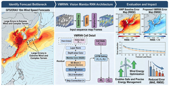
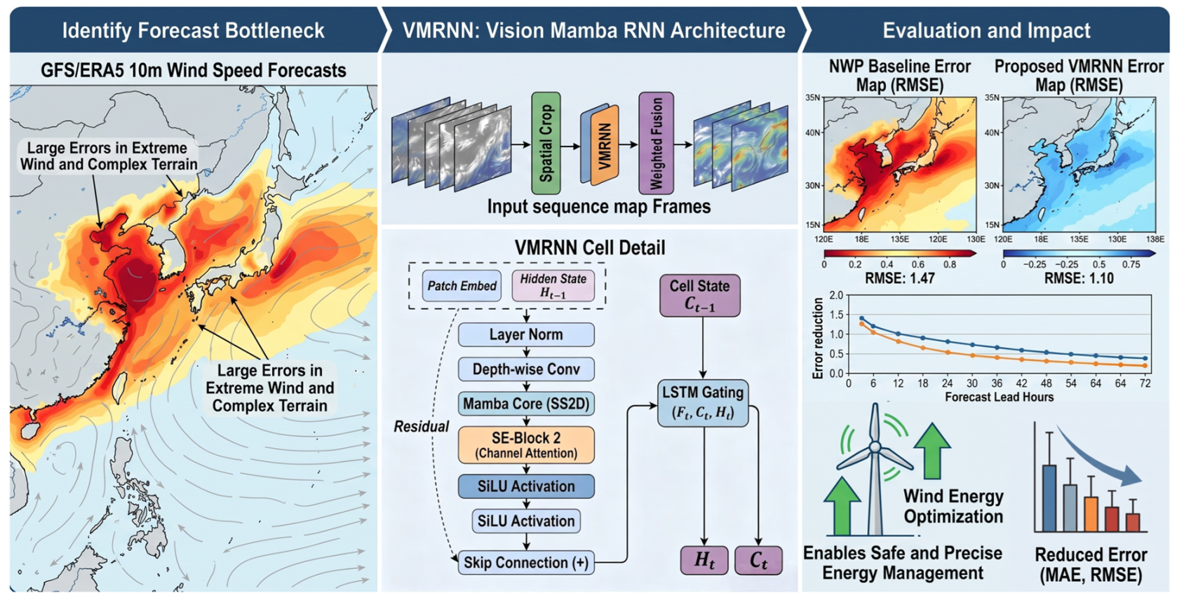
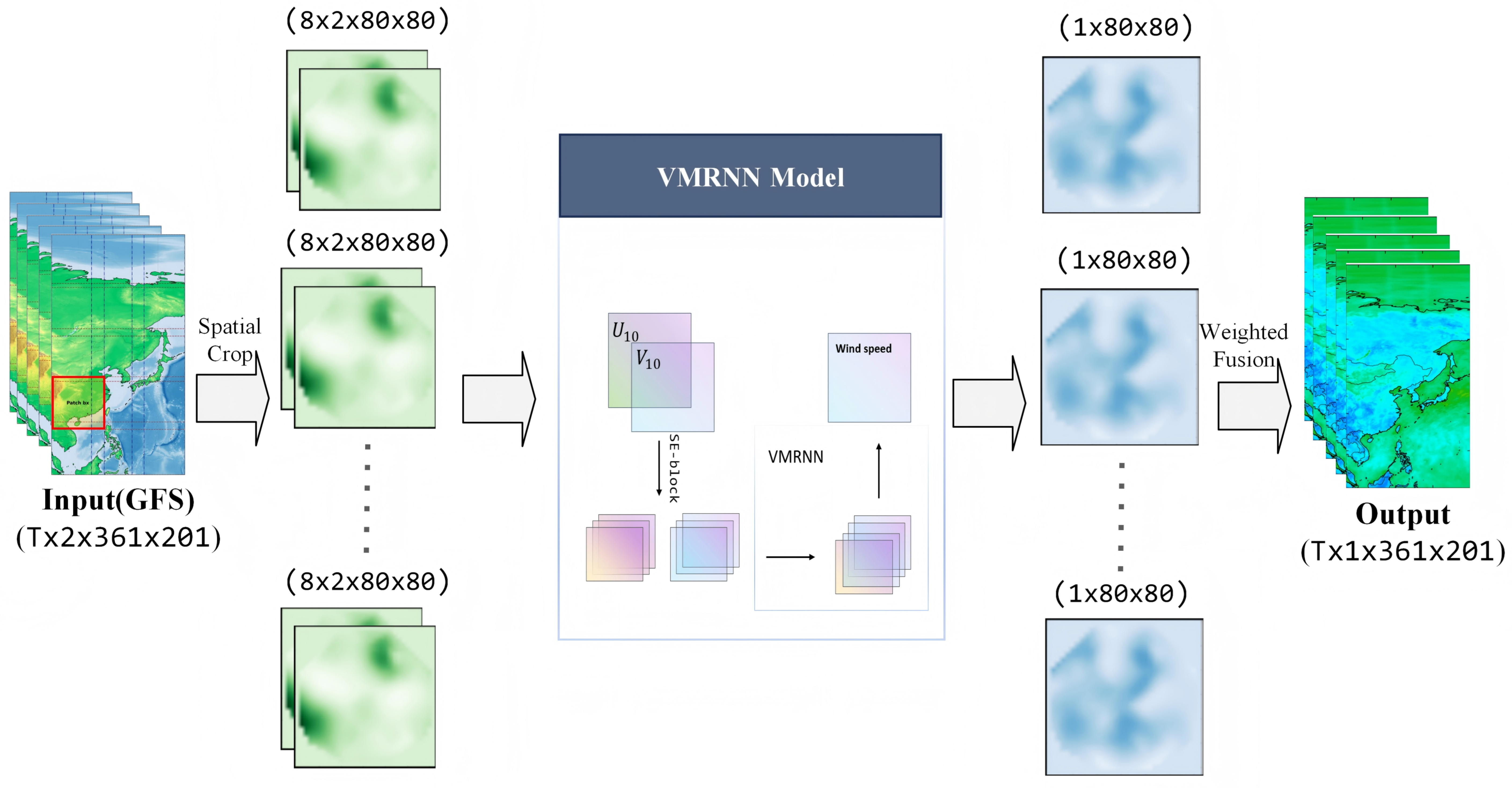
To further enhance wind speed forecast accuracy, this study proposes a spatiotemporal deep learning post-processing framework based on an improved Vision Mamba Recurrent Neural Network (VMRNN) to rectify 0–72 h NWP wind speed forecasts over the Northwest Pacific and its adjacent regions (Figure 1). Utilizing high-resolution GFS forecasts as inputs and ERA5 reanalysis data as the target truth, the framework was trained on a historical dataset spanning the past five years. Furthermore, the performance of the proposed framework was evaluated and compared against contemporary mainstream spatiotemporal baseline models, specifically SimVP [45] and SA-ConvLSTM [46].

2. Data and Methods

2.1. Study Area and Datasets

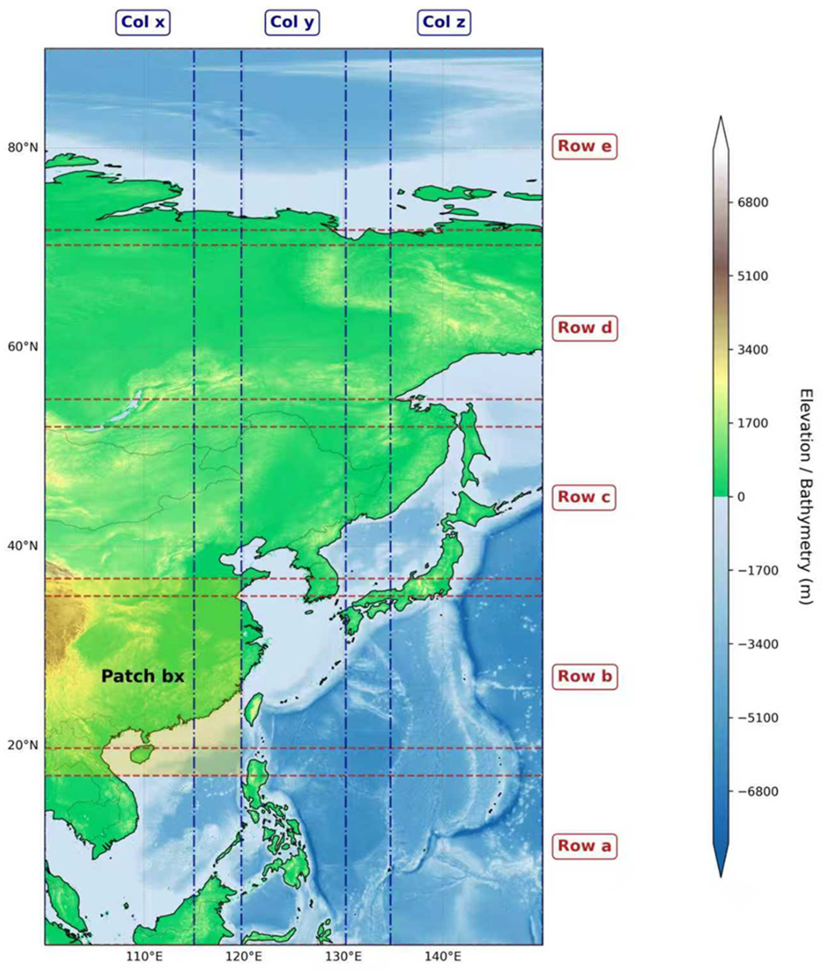
As illustrated in Figure 2, this research focuses on East Asia and the Northwest Pacific sector (0–90° N, 100–150° E), a region characterized by complex land–sea boundaries and frequent extreme marine weather events [47]. For model input, we utilized numerical forecast data from the National Centers for Environmental Prediction (NCEP, College Park, MD, USA) Global Forecast System (GFS). To comprehensively capture the vector characteristics of the wind field, the 10 m zonal wind (U-component) and 10 m meridional wind (V-component) were extracted as two-channel input sequence-to-one features. The forecast spans a lead time of 0–72 h with a temporal resolution of 3 h and a spatial resolution of 0.25°. Regarding the target labels, the ERA5 high-resolution reanalysis wind speed from the European Centre for Medium-Range Weather Forecasts (ECMWF, Reading, UK) was adopted as the ground truth for model training. The dataset was partitioned into two subsets: data from 2020 to 2024 were used for model training and validation, while data from 2024 to 2025 served as an independent test set for performance evaluation.

2.2. Data Preprocessing and Spatiotemporal Sliding Window Strategy

The original meteorological grid has a resolution of 361 × 201. To address the substantial memory demands of large-scale, long-lead-time spatiotemporal forecasting, this study designs a data reconstruction strategy that integrates spatial patching and a temporal sliding window.

In the spatial dimension, given the 0.25° resolution of the GFS model, an $80\times 80$ patch covers an actual physical ocean area of approximately 2000 km × 2000 km. This spatial coverage aligns with the classical synoptic scale in meteorology [3,48]. For the complex ocean environment of the Northwest Pacific, where typhoons occur frequently, a synoptic-scale spatial patch ensures that the physical integrity of large-scale weather systems (such as tropical cyclones and subtropical highs, which typically range from 500 to 1500 km in diameter) can be contained within a single receptive field [49]. Concurrently, to mitigate boundary artifacts induced by rigid grid segmentation, a sliding window strategy with 5 × 3 patches and spatial overlap was implemented. As illustrated in Figure 2 and

Table 1. Spatial patching strategy for the regional segmentation of the study area.

Rows	Latitude	Cols	Longitude
a	0.00° N–19.75° N	x	100.00° E–119.75° E
b	17.00° N–36.75° N	y	115.00° E–134.75° E
c	35.00° N–54.75° N	z	130.25° E–150.00° E
d	52.00° N–71.75° N	-	-
e	70.25° N–90.00° N	-	-

, the target region is partitioned into multiple 80$\times$80 local spatial patches, with a predefined overlap maintained between adjacent patches. Each patch is independently processed by the model for prediction. Subsequently, the outputs are seamlessly fused into a 361 × 201 global forecast field through a weighted average of the overlapping regions, effectively eliminating spatial discontinuities.

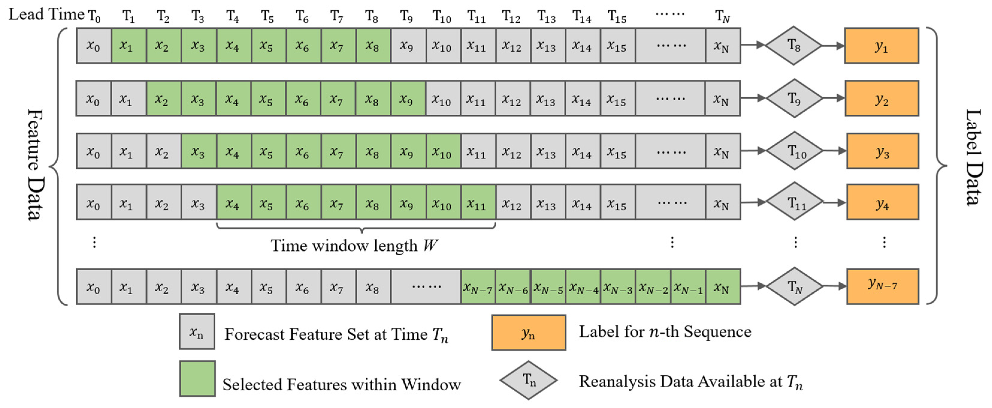
In the temporal dimension, the eight forecast time steps (with a 3 h interval per step) correspond strictly to a complete 24 h atmospheric diurnal cycle. The evolution of wind fields within the marine atmospheric boundary layer is strongly influenced by the diurnal variations of solar radiative thermal forcing and the thermal circulation of land–sea breezes; however, traditional NWP models frequently exhibit systematic phase lags in characterizing these diurnal variations [50,51]. By utilizing a 24 h sliding temporal window, the proposed model can continuously encode the thermodynamic evolutionary trajectories over a full preceding day and night within its long- and short-term memory states, thereby adaptively rectifying the phase biases of NWP models in predicting wind field diurnal cycles [11] (Figure 3). The model takes as input the U and V forecast fields at the target time step and the seven preceding steps (at a temporal resolution of 3 h), yielding an input shape of (8, 80, 80, 2). This tensor is used to derive the gridded wind speed field at the target lead time with an output shape of (80, 80, 1). By shifting the window sequentially along the time axis, full-lead-time wind field correction from 0 to 72 h is achieved.

2.3. Baseline Models

This study selects two mainstream spatiotemporal forecasting architectures as baseline models for comparison: SA-ConvLST [46], which is based on a recurrent neural network mechanism, and SimVP [45], which is based on a pure convolutional architecture.

The primary rationale for selecting these two models is that they represent two core technical paradigms in the current field of deep learning for spatiotemporal meteorological forecasting:

• SA-ConvLSTM represents the classic “RNN + Attention” paradigm. Traditional Convolutional Long Short-Term Memory (ConvLSTM) is constrained by the local receptive fields of convolutional kernels, making it difficult to capture large-scale spatial dependencies. By introducing a self-attention mechanism, SA-ConvLSTM can effectively extract long-range spatial topological features on a global scale.
• SimVP represents the “recurrent-free” pure convolutional paradigm. It completely discards the RNN structure and extracts spatiotemporal features through a pure encoder–decoder design, resulting in exceptionally high computational efficiency.

2.4. Introduction of the VMRNN Model

Although the aforementioned mainstream models have made significant progress in short-term meteorological forecasting, they still face inherent structural bottlenecks when applied to high-resolution, long-lead-time (0–72 h) sea surface wind field forecasting over the Northwest Pacific. On the one hand, models based on self-attention mechanisms, such as SA-ConvLSTM, suffer from quadratically increasing computational complexity as spatial resolution increases, leading to prohibitive memory overhead that is impractical for high-resolution grids. On the other hand, pure convolutional architectures like SimVP lack explicit temporal memory modules, making it difficult to accurately characterize the long-term nonlinear dynamical features during the evolution of complex weather systems.

To overcome this dual bottleneck of computational efficiency and long-range spatiotemporal modeling capability, this study introduces and improves the VMRNN model. This architecture integrates the efficient spatial feature extraction capability of Vision Mamba with the long- and short-term temporal memory (LSTM) mechanism [37], providing an ideal solution for the dynamic spatiotemporal correction of large-scale ocean wind fields [52].

2.4.1. Selective State Space Mechanism of the VMRNN Model

The core components of the VMRNN model are formulated based on discretized State Space Models (SSMs). To overcome the limitations of traditional SSMs—namely, their static parameters and the consequent difficulty in capturing complex, nonlinear meteorological sequences—VMRNN incorporates a selective state-space mechanism (Selective SSMs, S6) [35]. Given an input sequence $x_t$ and the corresponding hidden state $h_t$, the discretization and subsequent state update process of this mechanism can be formulated as follows [53]:

$$h_t=\overline{A}{h}_{t-1}+\overline{B}{x}_t$$

(1)

$$y_t=\overline{C}{h}_t$$

(2)

Unlike traditional static systems, the distinguishing feature of the S6 mechanism is that its state transition parameter $\overline{B}$, output parameter $\overline{C}$, and discretized time step $\Delta$ are established as functions that vary dynamically with the input feature $x_t$:

$$S_B=\mathrm{Linear}(x_t), S_C=\mathrm{Linear}(x_t), S_{\Delta }=\mathrm{softplus}(\mathrm{Linear}(x_t))$$

(3)

where $S_B$, $S_C$, and $S_{\Delta }$ are the outputs of the linear projection layers; $\mathrm{L}\mathrm{i}\mathrm{n}\mathrm{e}\mathrm{a}\mathrm{r}$ denotes a linear projection layer; and $\mathrm{s}\mathrm{o}\mathrm{f}\mathrm{t}\mathrm{p}\mathrm{l}\mathrm{u}\mathrm{s}$ represents the activation function that ensures the positive definiteness of the time step [54]. From a physical perspective, this input-dependent dynamic parameterization endows the model with a “selective filtering” capability. When processing the large-scale evolution of wind fields over the Northwest Pacific, the model can adaptively adjust the retention and forgetting weights of historical meteorological information based on the local wind dynamical characteristics of the grid. This facilitates a comprehensive representation of the spatiotemporal evolution of the wind field while maintaining linear computational complexity [55].

2.4.2. Channel Attention Mechanism (SE-Block)

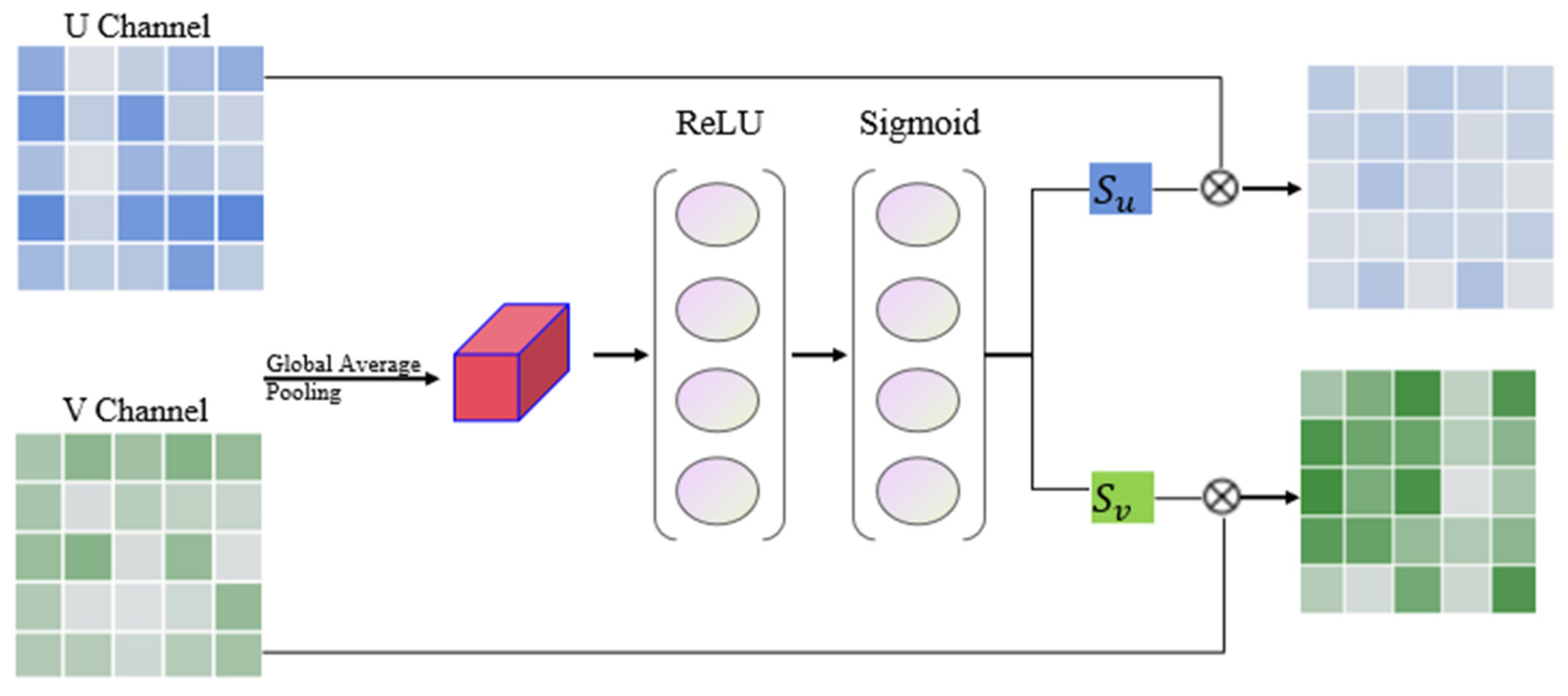
Considering the inherent physical dynamical coupling (such as geostrophic balance and boundary layer friction) between the zonal ($U$) and meridional ($V$) components of the sea surface wind field, this study incorporates a channel attention mechanism (Squeeze-and-Excitation block, SE-Block) into the architecture to adaptively capture this nonlinear relationship. Mathematically, given an input feature map $X\in {\mathbb{R}}^{C\times H\times W}$ (where the channel dimension $C=2$ represents the $U$ and $V$ components, respectively), the SE-Block first compresses the spatial dimensions into a feature vector $Z\in {\mathbb{R}}^C$ via global average pooling, which serves as a global descriptor characterizing the fluid domain. Subsequently, a two-layer multilayer perceptron (MLP) learns the nonlinear dynamic weights $S$ for each channel, which are then applied channel-wise to the original feature map to achieve feature recalibration (Figure 4):

$$S_c=\sigma (W_2\delta (W_1{Z}_c))$$

(4)

$${\tilde{X}}_c=S_c\cdot X_c$$

(5)

where $\delta$ denotes the Rectified Linear Unit (ReLU) activation function, $\mathrm{\sigma }$ represents the Sigmoid normalization function that constrains the weights within the interval (0, 1), and $W_1$ and $W_2$ are the weight matrices of the fully connected layers. ${\tilde{X}}_c$ represents the recalibrated feature output for the $c$ channel, and $S_c$ is the channel weight obtained from the excitation stage. Through this formulation, the model adaptively allocates importance weights between the $U$ and $V$ physical channels, thereby facilitating the integration of underlying dynamical interactions between the orthogonal wind components.

2.4.3. VMRNN Architecture Integrated with Channel Attention

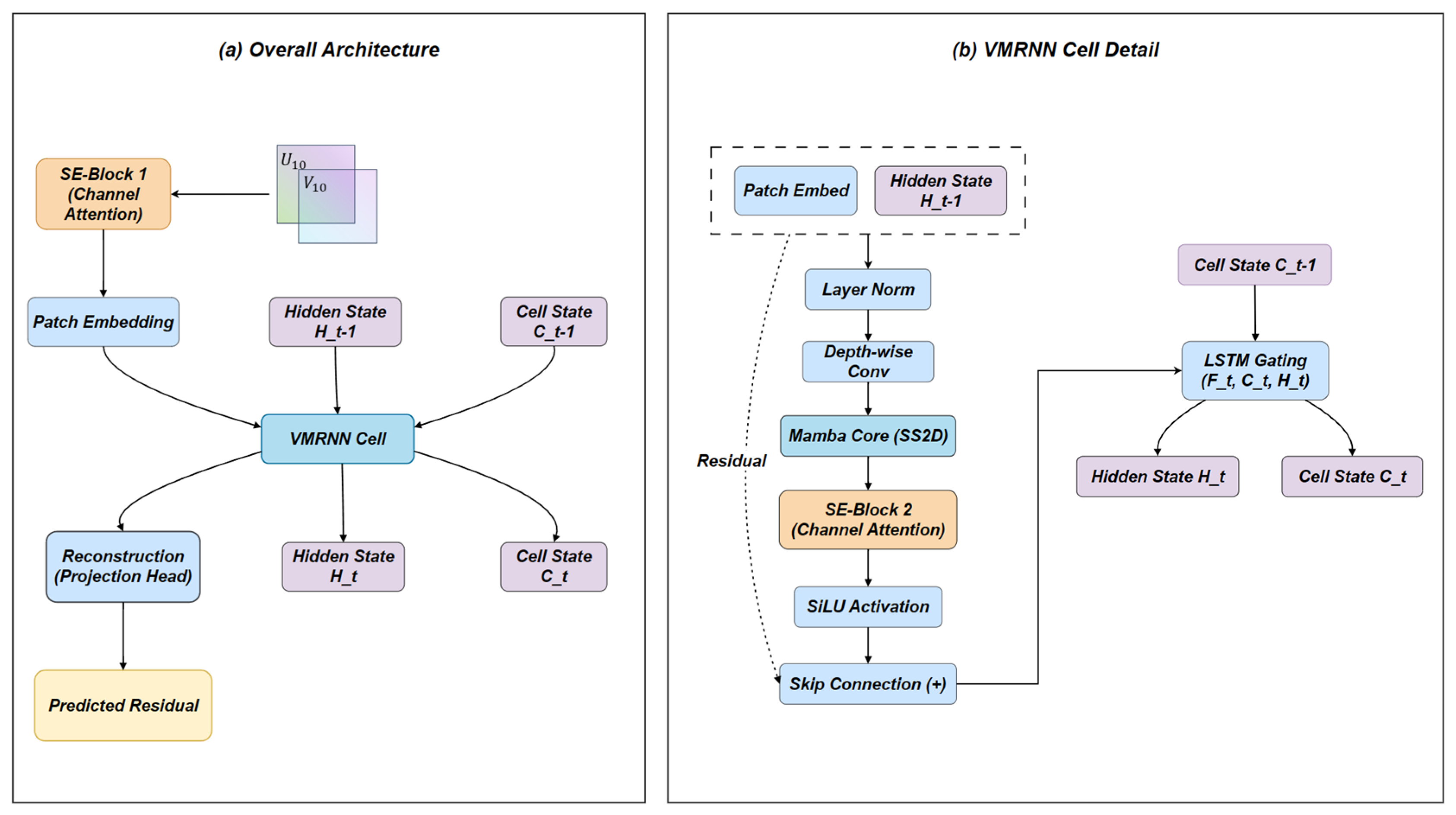
The proposed model architecture, illustrated in Figure 5, integrates the SE channel attention module to capture the complex nonlinear dynamical coupling between the orthogonal U and V wind components. As shown in Figure 5a, the dual-channel input (U, V) first passes through SE-Block 1 for initial recalibration before entering the Patch Embedding layer.

Within the VMRNN Cell (Figure 5b), the features undergo layer normalization and depth-wise convolution to encode local spatial contexts. The features are then processed by the Mamba Core (utilizing the 2D Selective Scan, SS2D module) for global spatiotemporal feature extraction. To further enhance feature representations, SE-Block 2 is deployed after the Mamba Core. Finally, the updated hidden state $H_t$ and cell state $C_t$ are generated through a residual connection and an LSTM gating mechanism to predict the wind field at the next time step.

2.5. Loss Function

At the reconstruction stage of the model, this study adopts a residual learning strategy. Large-scale sea surface wind fields exhibit a high degree of fluid dynamical consistency, and NWP models have already captured the large-scale fluid dynamical framework—such as geostrophic winds and pressure gradient forces—through their underlying partial differential dynamical cores. Direct prediction of absolute wind fields by a deep learning model is prone to disrupting the inherent atmospheric dynamical balance of the NWP, potentially leading to physical distortions [56]. From the perspective of atmospheric physics, the residual essentially represents the systematic biases induced by unresolved subgrid-scale processes within the NWP model. Through residual regression, the deep learning model functions primarily as a “subgrid physical compensator”. By utilizing the large-scale fluid evolution of the NWP model as the background field, it focuses on compensating for nonlinear biases at the subgrid scale. This bias correction framework not only accelerates the convergence of the deep network but also effectively preserves the physical constraints and dynamical consistency of the corrected wind field [57].

Let $V_{NWP,i}$ be the target-time numerical forecast input at the grid point $i$ and $V_{ERA5,i}$ be the corresponding ground-truth value. The target residual ${ϵ}_i$ is defined as follows:

$${ϵ}_i=V_{NWP,i}-V_{ERA5,i}$$

(6)

During the training phase, the Root Mean Square Error (RMSE) of the residuals is employed as the loss function to optimize the model’s performance:

$$Loss=\sqrt{{\displaystyle \frac{1}{N}}{\displaystyle \sum _{i=1}^N{({ϵ}_i-{\widehat{ϵ}}_i)}^2}}$$

(7)

Here, $N$ denotes the total number of evaluation grid samples, and $\widehat{{ϵ}_{\mathrm{i}}}$ represents the predicted residual output by the VMRNN model.

By minimizing this residual loss, the deep learning network is compelled to focus exclusively on extracting underlying systematic bias patterns within the numerical model, thereby enhancing convergence efficiency and prediction accuracy in meteorological post-processing tasks.

3. Experiments and Results

3.1. Parameter Settings and Evaluation Metrics

The model training and testing were conducted on an NVIDIA V100 GPU platform (NVIDIA, Santa Clara, CA, USA). The hyperparameters for the VMRNN model were configured as follows: the number of input channels was set to 2, the patch size to 2, the embedding dimension to 128, and the depth of VSS blocks to 6. Training was performed for 150 epochs with a batch size of 100 using the Adam optimizer, with an initial learning rate of 0.0001.

To objectively quantify the correction performance of each model for the NWP-predicted wind speeds, this study selected four core statistical metrics commonly used in meteorology: Mean Absolute Error (MAE), Root Mean Square Error (RMSE), systematic Mean Bias (BIAS), and Percentage Bias (PBIAS). These metrics are defined as follows:

$$MAE={\displaystyle \frac{1}{N}}{\displaystyle \sum _{i=1}^N|}{F}_i-O_i|$$

(8)

$$RMSE=\sqrt{{\displaystyle \frac{1}{N}}{\displaystyle \sum _{i=1}^N{(F_i-O_i)}^2}}$$

(9)

$$BIAS={\displaystyle \frac{1}{N}}{\displaystyle \sum _{i=1}^N(F_i-O_i)}$$

(10)

$$\mathrm{PBIAS}={\displaystyle \frac{{\displaystyle \sum _{i=1}^N(F_i-O_i)}}{{\displaystyle \sum _{i=1}^N{O}_i}}}\times 100\%$$

(11)

Here, $N$ denotes the total number of evaluation grid samples, $F_i$ represents the model-predicted wind speed at the grid point $i$ after post-processing, and $O_i$ is the corresponding ERA5 ground truth value. Concurrently, this study introduces the coefficient of determination ${\mathrm{R}}^2$ and Spearman’s rank correlation coefficient as auxiliary evaluation metrics for spatial scatter density distribution. Specifically, the Spearman coefficient is utilized to assess the monotonic consistency between forecasted values and target observations under extreme nonlinear distributions. All correlation metrics are evaluated using a two-sided test to calculate the p-value, thereby rigorously verifying their statistical significance.

In addition to the absolute numerical deviations, this study introduced the Pattern Correlation Coefficient (PCC) to evaluate the similarity in spatial topological structure between the predicted and observed wind fields. The PCC measures the degree of linear correlation in the spatial distribution patterns; a value closer to 1 indicates a more accurate characterization of large-scale atmospheric circulation. It is defined as

$$PCC={\displaystyle \frac{{\displaystyle \sum _{i=1}^N(F_i-\overline{F})}(O_i-\overline{O})}{\sqrt{{\displaystyle \sum _{i=1}^N{(F_i-\overline{F})}^2}}\sqrt{{\displaystyle \sum _{i=1}^N{(O_i-\overline{O})}^2}}}}$$

(12)

where $\overline{F}$ and $\overline{O}$ represent the spatial mean values of the predicted and observed wind speeds, respectively.

To specifically assess the models’ early warning capability for extreme weather, this study employed the binary classification contingency table verification method recommended by the World Meteorological Organization (WMO) for specific wind speed thresholds. After setting a threshold, $N_H$ is defined as the number of correct hits, $N_F$ as the number of false alarms (where the forecast reaches the threshold, but the observation does not), and $N_M$ as the number of misses (where the observation reaches the threshold, but the forecast does not). Based on these, two core categorical indicators were utilized:

Threat Score (TS): A comprehensive metric considering hits, false alarms, and misses. It is the most rigorous and widely used indicator for evaluating extreme weather area forecast accuracy, with values ranging from 0 to 1:

$$TS={\displaystyle \frac{N_H}{N_H+N_F+N_M}}$$

(13)

False Alarm Ratio (FAR): This measures the proportion of samples where a gale was predicted but did not actually occur. FAR directly reflects the model’s tendency for over-prediction:

$$FAR={\displaystyle \frac{N_F}{N_H+N_F}}$$

(14)

3.2. Performance Comparison Across Different Lead Times

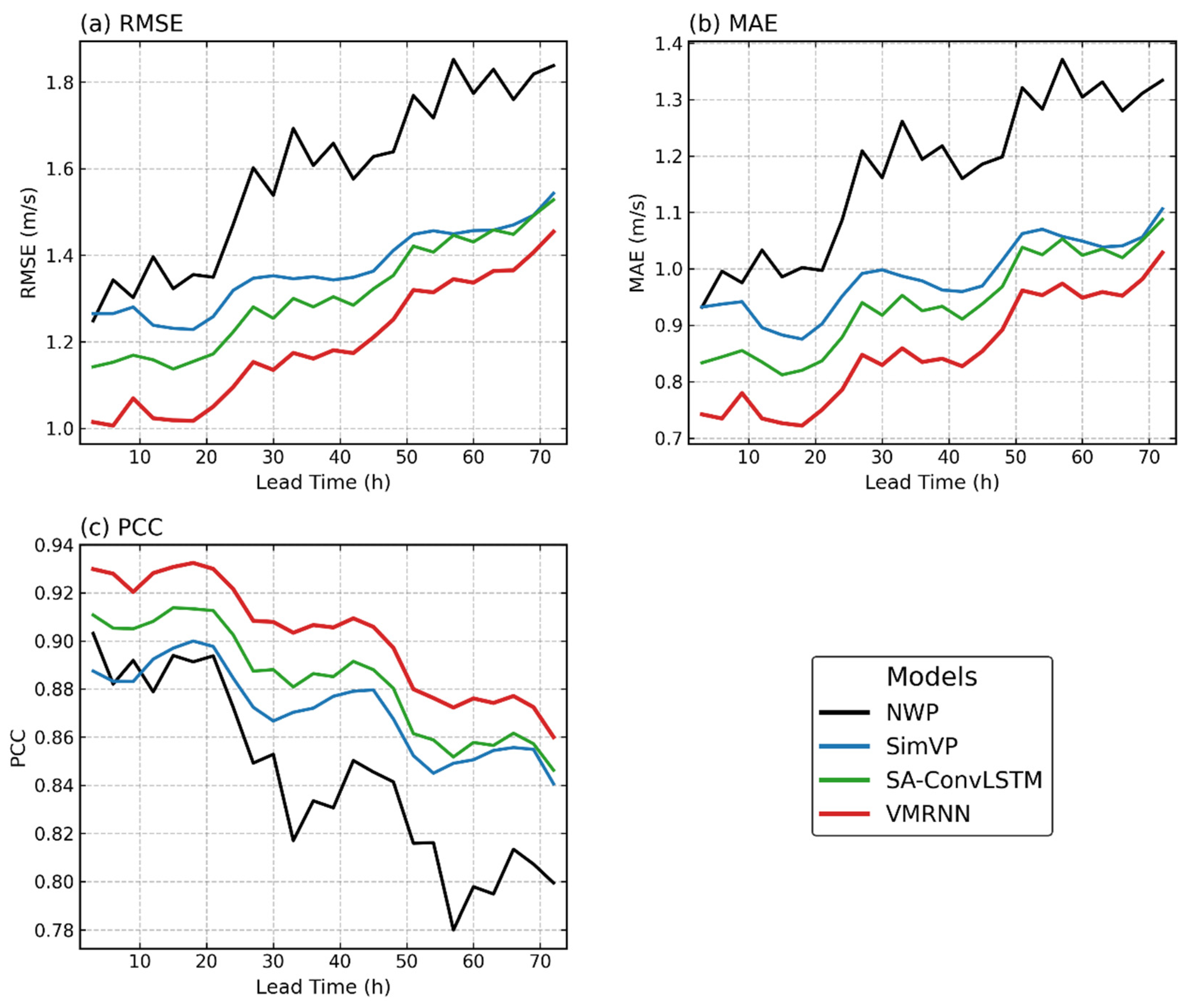
To comprehensively evaluate the forecasting performance of various models for the wind field in the Northwest Pacific region, this study utilized three quantitative metrics—Root Mean Square Error (RMSE), Mean Absolute Error (MAE), and the Pattern Correlation Coefficient (PCC)—to systematically compare the numerical weather prediction (NWP) forecasts with three deep learning correction models (SimVP, SA-ConvLSTM, and VMRNN) for lead times ranging from 0 to 72 h. Figure 6 illustrates the evolutionary trends of these evaluation metrics as a function of the forecast lead time.

As shown in Figure 6a,b, the errors of the original NWP forecasts exhibit a rapid and continuous growth trend as the lead time extends. Specifically, as summarized in

Table 2. Quantitative comparison of forecasting performance among NWP and different deep learning models at key lead times (24 h, 48 h, and 72 h). (The bold values indicate the best performance for each metric).

	Lead Time	NWP	SimVP	SA-ConvLSTM	VMRNN
RMSE (m/s)	24 h	1.47	1.32	1.22	1.10
	48 h	1.64	1.41	1.35	1.25
	72 h	1.84	1.54	1.53	1.45
MAE (m/s)	24 h	1.09	0.95	0.88	0.79
	48 h	1.20	1.02	0.97	0.89
	72 h	1.33	1.11	1.09	1.03
PBIAS (%)	24 h	−5.95	−1.34	−0.56	−0.34
	48 h	−6.53	−1.87	−1.13	−0.91
	72 h	−6.91	−2.19	−1.48	−1.30
PCC	24 h	0.87	0.88	0.90	0.92
	48 h	0.84	0.87	0.88	0.90
	72 h	0.80	0.84	0.85	0.86

, the RMSE of the NWP increases from 1.47 m/s at 24 h to 1.84 m/s at 72 h, and the MAE rises from 1.09 m/s to 1.33 m/s, highlighting significant dynamical error accumulation in traditional numerical models during long-term integration. In contrast, the implementation of deep learning post-processing modules effectively slowed the rate of error growth, demonstrating consistent denoising and correction capabilities across all evaluated models.

Among the models assessed, VMRNN consistently demonstrated superior performance in reducing absolute wind speed errors. It maintained the lowest error throughout the 72 h forecast cycle. As detailed in Table 2, at the 24 h lead time, the RMSE of VMRNN is only 1.10 m/s, representing a reduction of 25.5% compared to the original NWP. Even at the 72 h lead time, VMRNN maintains the RMSE at 1.45 m/s, a 20.9% improvement over the NWP. In terms of the MAE, VMRNN achieved substantial reductions ranging from 22% to 27%. Compared to the SimVP and SA-ConvLSTM deep learning baselines, VMRNN consistently provided superior correction results, validating its high effectiveness in extracting complex meteorological spatiotemporal features.

Beyond the accuracy of absolute wind speed values, maintaining spatial consistency between forecasted and ground-truth wind fields is critical for maritime disaster prevention and mitigation. The PCC results for each model are presented in Figure 6c and Table 2. The PCC of the NWP decreases markedly over time, falling to 0.80 at 72 h, which indicates a significant distortion in the spatial structure of its forecasted wind field. Notably, the VMRNN model demonstrates strong robustness in preserving the spatial structure while controlling numerical errors. Its PCC reaches 0.92 at 24 h and remains as high as 0.86 at 72 h. These results suggest that VMRNN effectively smooths and corrects wind speed magnitudes while accurately retaining the large-scale spatial topological features of the real wind field.

VMRNN also demonstrates favorable capability in mitigating the systematic biases of the numerical models. As shown in Table 2, the raw NWP forecasts exhibit a persistent systematic underestimation tendency, with the Percentage Bias (PBIAS) deteriorating from −5.95% at the 24 h lead time to −6.91% at 72 h. Following the implementation of deep learning post-processing, all baseline models alleviate this underestimation tendency to varying degrees. Among them, VMRNN exhibits the most substantial bias reduction, converging the PBIAS to −0.34% in the 24 h forecasts and yielding a nearly unbiased prediction; even during the 72 h long-lead-time integration, its PBIAS remains at −1.30%, outperforming the SimVP and SA-ConvLSTM models. These results indicate the effectiveness of the proposed framework in mitigating the underlying non-uniform systematic biases.

3.3. Spatial Distribution Characteristics of Errors

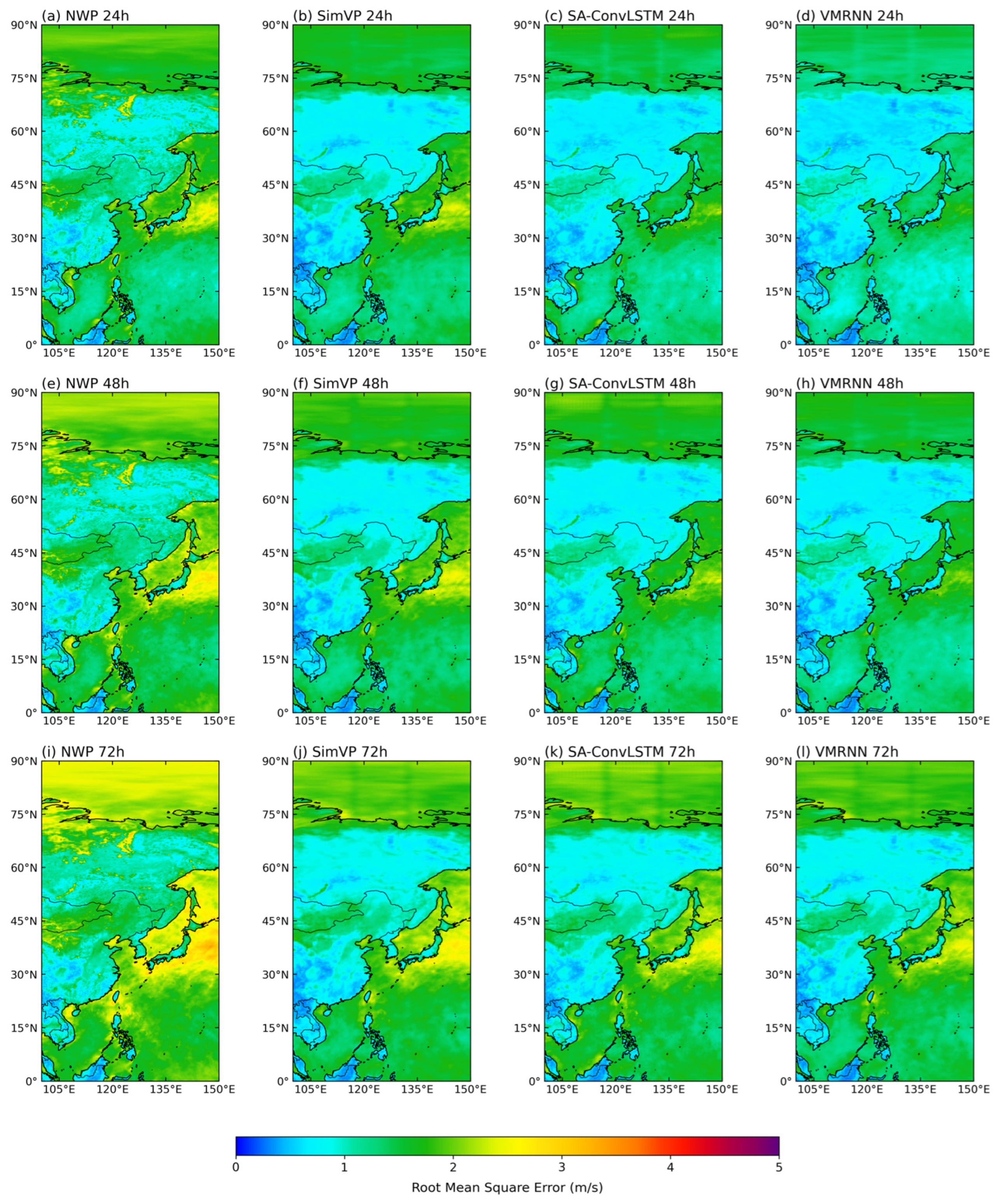
To further investigate the spatial discrepancies in forecasting performance and the evolution of errors across different models, this study plotted the spatial distribution of the Root Mean Square Error (RMSE) for the NWP and the three deep learning correction models at lead times of 24 h, 48 h, and 72 h (Figure 7). By comparing the error distribution characteristics within the study area, the adaptability of each model to complex geographical and meteorological conditions can be intuitively evaluated.

Observing the NWP forecast results (Figure 7a,e,i), it is evident that while the errors are relatively small in the initial stage (24 h), they exhibit significant spatial propagation and non-uniform accumulation as the lead time extends. At the 72 h lead time (Figure 7i), the NWP displays extensive high-error zones (indicated by yellow and orange patches). These extreme error regions are primarily concentrated in two types of geographical locations: first, over mid-to-high latitude oceans (e.g., the ocean east of Japan, the Sea of Okhotsk, and parts of the Bering Sea), which are frequently influenced by extratropical cyclone activities in the westerlies, leading to intense non-linear wind field variations; second, along complex land–sea boundaries and topographical edges (e.g., the eastern coast of China and high-altitude regions). In these areas, NWP parameterization schemes struggle to accurately resolve subgrid-scale dynamical processes due to differences in land–sea thermal properties and frictional effects, resulting in severe deviations between predicted wind speeds and actual observations.

In comparison, all deep learning models suppressed the rapid spatial propagation of NWP errors to varying degrees. Although SimVP (Figure 7j) and SA-ConvLSTM (Figure 7k) effectively reduced the extreme error peaks over high-latitude oceans in 72 h forecasts, residual moderate-error zones remained in some mid-latitude sea areas and continental regions. This suggests that these models still lack sufficient capacity to capture large-scale atmospheric background fields during long-lead-time integration.

In contrast, the VMRNN model demonstrated superior spatial error control capabilities. Across both short-term (24 h) and long-term (72 h) integrations, the spatial distribution of RMSE for VMRNN (Figure 7d,h,i) remained consistently low and highly smoothed. Furthermore, VMRNN effectively eliminated the large-value error patches produced by the NWP at land–sea interfaces and mid-to-high-latitude oceans. These results indicate that VMRNN can not only extract and memorize the spatiotemporal evolutionary features of meteorological elements but also adaptively learn and correct the systematic spatial biases inherent in the NWP’s underlying physics, particularly those arising from complex boundary layer friction and sea–land thermal exchanges. By mitigating these localized extreme error sources, VMRNN successfully maintains the error field at a stable and uniform low level across the entire study area, significantly enhancing the spatial reliability of wind field forecasts.

3.4. Error Distribution Patterns and Systematic Bias Correction

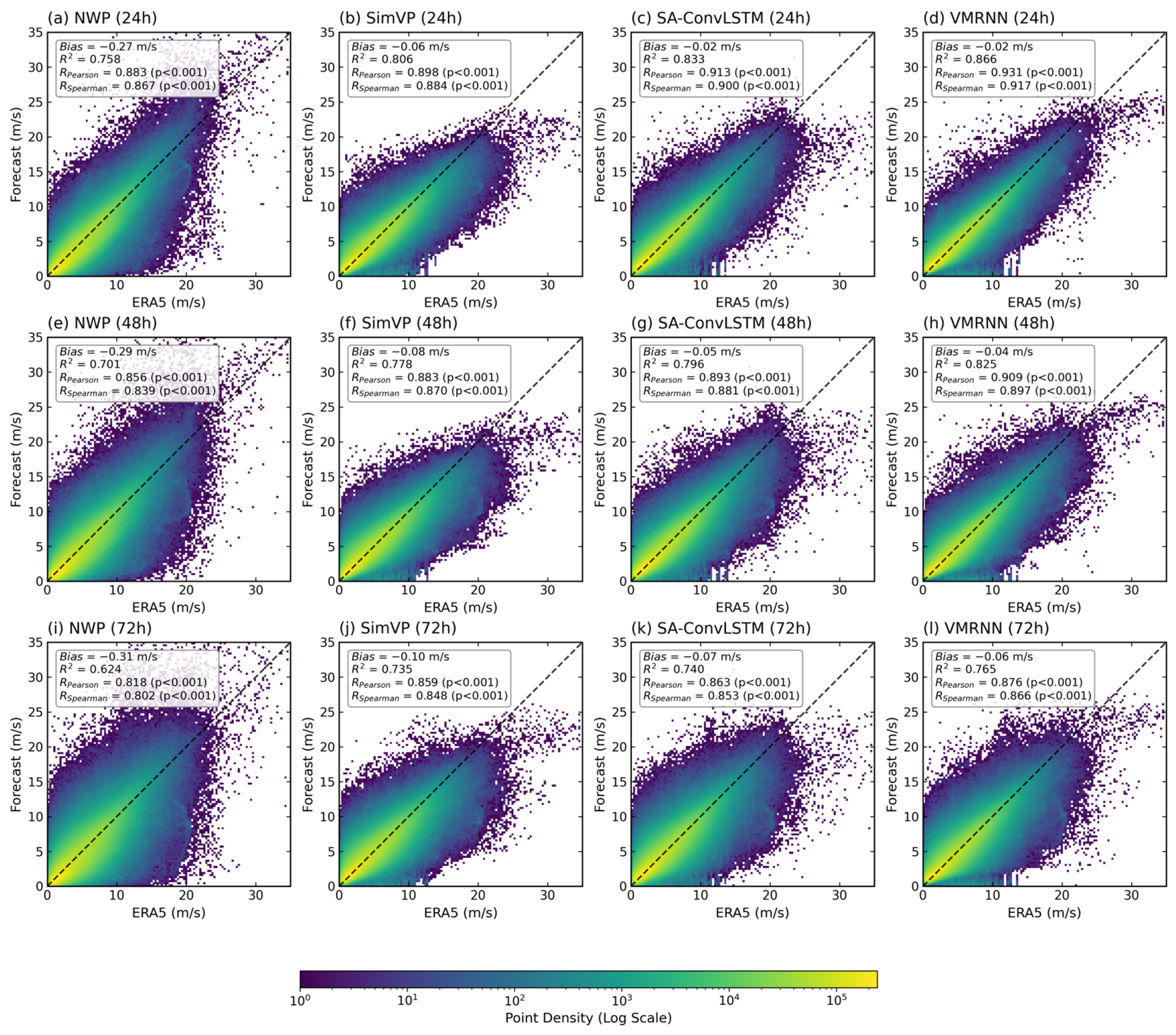
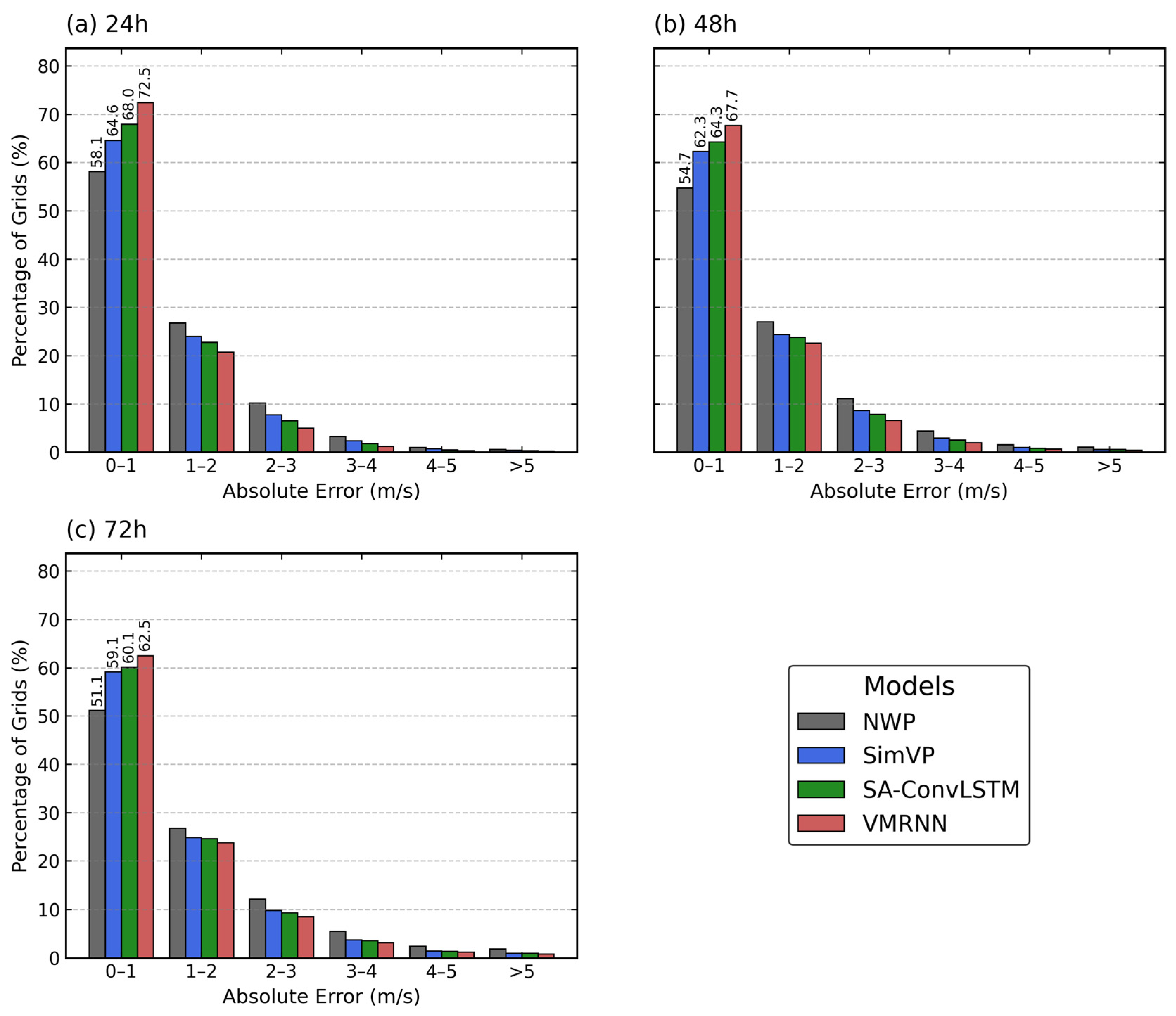
The preceding overall metrics and spatial distribution results demonstrate that VMRNN significantly reduces wind field forecasting errors. To investigate the underlying statistical mechanisms through which the model corrects NWP errors across different lead times, observation-forecast scatter density plots (Figure 8) and absolute error distribution histograms (Figure 9) were generated.

In Figure 8, for an ideal unbiased forecasting model, the scatter points should be highly concentrated along the $y = x$ diagonal. Observing the scatter density distribution reveals that the original NWP forecasts exhibit a pronounced “non-uniform bias” across different wind speed regimes. In the low-to-medium wind speed regime (≤15 m/s), the center of gravity of the NWP’s high-density scatter cloud deviates toward the lower right of the diagonal, indicating a prevalent underestimation. Conversely, in the high wind speed regime (>15 m/s), the NWP displays significant overestimation and strong dispersion. Because low-to-medium wind speed samples constitute the absolute majority in the climatology, their underestimation effect dominates the overall error, resulting in a negative systematic bias for the NWP. Taking the 24 h forecast as an example, the coefficient of determination ${\mathrm{R}}^2$ of the NWP is 0.758, with a Bias of −0.27 m/s.

As seen in Figure 8, all deep learning models show significant improvements relative to the NWP forecasts, with VMRNN performing the best. In the core low-to-medium wind speed regime, VMRNN’s scatter cloud closely aligns with the $y = x$ diagonal, effectively mitigating the NWP’s underestimation tendency and bringing the overall forecast bias close to zero (Bias = −0.02 m/s). In the high wind speed regime, constrained by the smoothing effect inherent in deep learning models optimized via mean square error (MSE), VMRNN exhibits a slight underestimation; however, by substantially reducing the overestimated false-alarm samples of the NWP, it markedly decreases the overall dispersion of the wind field forecasts. Specifically, in the 24 h forecast, VMRNN increases the coefficient of determination ${\mathrm{R}}^2$ from 0.758 (NWP) to 0.866; concurrently, accounting for the nonlinear distribution of extreme winds, VMRNN improves Spearman’s rank correlation coefficient from 0.867 to 0.917. Given the large grid sample size of the high-resolution meteorological fields, all correlation tests illustrated in the figure exhibit high statistical significance (p < 0.001). The comprehensive improvement in these statistical metrics demonstrates that the model does not merely perform a simple global translation; rather, by capturing complex nonlinear spatiotemporal features, it achieves adaptive, dynamic bias correction across different wind speed regimes.

The elimination of systematic bias and the reduction in variance directly lead to a significant increase in the proportion of high-accuracy forecast samples. This error convergence effect is intuitively reflected in the absolute error distribution histograms. As shown in Figure 9, the VMRNN model significantly reduces the proportion of grids in the medium-to-high error intervals (≥2 m/s) and effectively shifts these largely deviated samples into the ultra-low error interval. For the 24 h short-term forecast, VMRNN substantially increases the proportion of high-accuracy samples (absolute errors between 0 and 1 m/s) to 72.5%, compared to 58.1% for the NWP. Even in the 72 h long-term forecast, where dynamical uncertainty is higher, VMRNN maintains excellent error control capability, with the proportion in the 0–1 m/s interval reaching 62.5% versus 51.1% for the NWP. This characteristic of concentrating the overall error distribution toward the low-error end demonstrates that VMRNN’s spatiotemporal correction capability persists throughout the entire life cycle of model integration, providing more stable and unbiased wind field forecasts for operational meteorology.

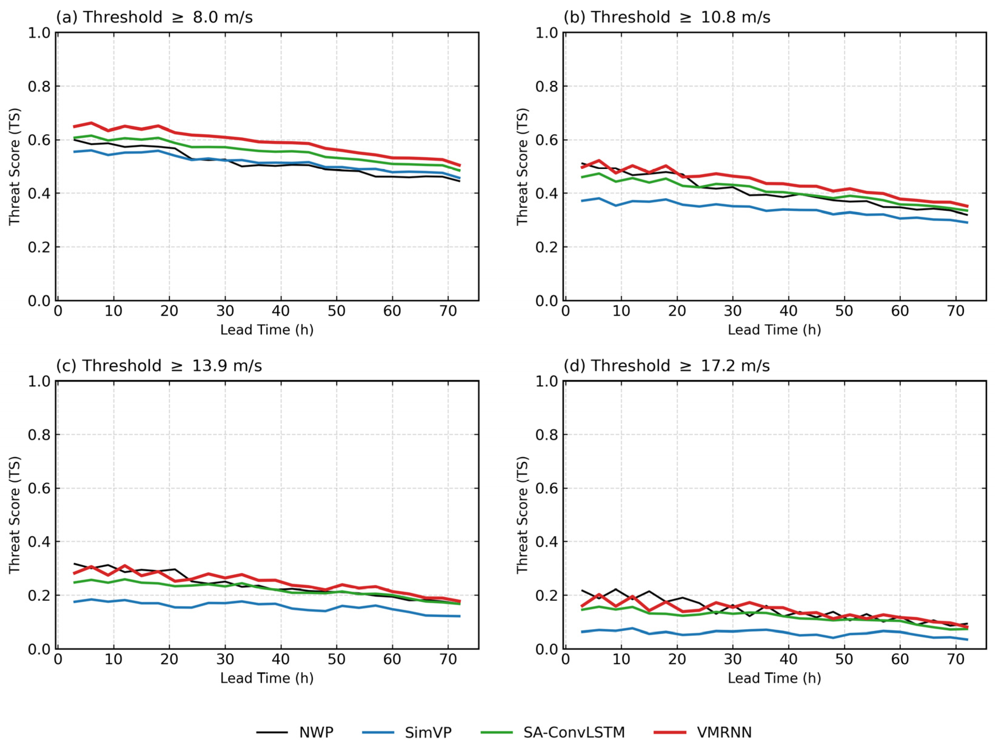
3.5. Categorical Forecast Evaluation at Different Wind Speed Thresholds

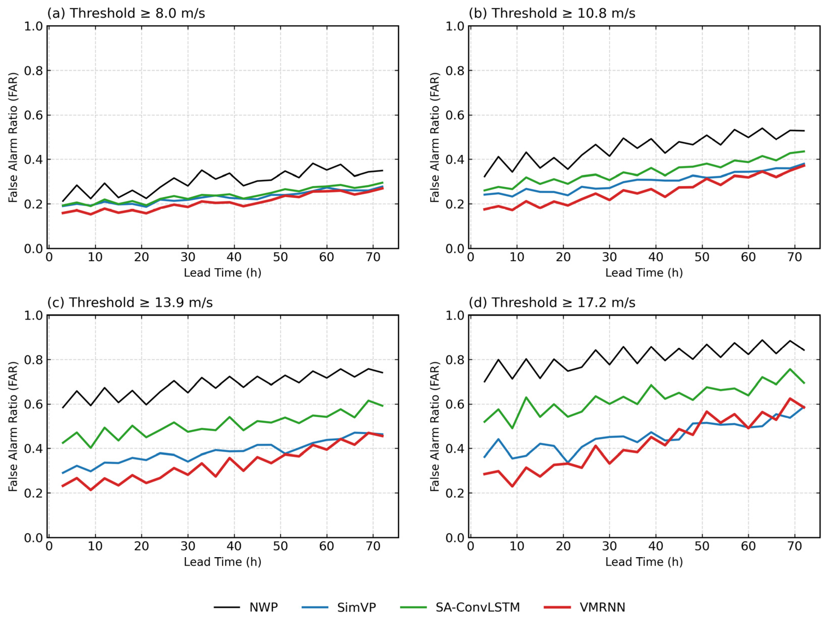
Beyond assessing overall numerical errors and spatial consistency, the model’s ability to characterize the impact areas of different gale levels (i.e., the extent of strong winds) is equally crucial for meteorological evaluation. This study selects four wind speed thresholds: 8.0, 10.8, 13.9, and 17.2 m/s (corresponding to Beaufort scales 5, 6, 7, and 8, respectively). Utilizing deterministic categorical verification methods, we calculated the Threat Score (TS) (Figure 10) and False Alarm Ratio (FAR) (Figure 11) for each model.

For the moderate wind speed thresholds of 8.0 m/s and 10.8 m/s (Figure 10a,b), the VMRNN model maintains high TS ratings throughout the entire 72 h forecast period. Simultaneously, as shown in Figure 11a,b, VMRNN achieves the lowest FAR among all evaluated models. This indicates that during typical gale events, VMRNN not only yields a high hit rate but also effectively suppresses the generation of false alarms, demonstrating high reliability in predicting the primary coverage of strong winds.

When the threshold increases to the high wind speed regimes of 13.9 m/s and 17.2 m/s, the evaluation reveals a significant over-prediction tendency in the traditional NWP model. As illustrated in Figure 10c,d, although the initial TS of the NWP is slightly higher than or comparable to some deep learning models, this hit rate comes at the cost of a severe false alarm penalty. Figure 11c,d show that the NWP exhibits notably high FAR values in extreme wind speed regimes. For instance, at the 17.2 m/s threshold for a 24 h lead time, the NWP’s FAR is approximately 0.75; at the 72 h lead time, this value approaches 0.90. This implies that a large proportion of the high-wind grids forecasted by the NWP do not actually reach the corresponding thresholds in observations, readily generating systematic spurious hazardous wind signals.

Overall, due to the error-averaging effect inherent in deep learning models, the absolute hit rates of SimVP and SA-ConvLSTM under certain high wind speeds are even lower than those of the NWP. In contrast, while VMRNN does not comprehensively surpass the NWP in initial absolute hit rates (TS) for extreme high winds, it achieves a substantial reduction in the false alarm ratio (FAR). For the 24 h forecast at the 17.2 m/s threshold, VMRNN successfully reduces the FAR from 0.75 (NWP) to 0.31; over the entire 72 h forecast cycle, VMRNN decreases the FAR by an average of 30–50% compared to the NWP.

4. Discussion

4.1. Performance of Spatiotemporal Forecasting Models

A comparison of multi-dimensional metrics reveals that, relative to the baseline models SimVP and SA-ConvLSTM, VMRNN mitigates the error accumulation inherent in traditional models during prolonged integration, leveraging the long-range memory mechanism of State Space Models (SSMs). In terms of absolute errors (Table 1), the model reduces the RMSE of the raw NWP by 25.5% (from 1.47 m/s to 1.10 m/s) in the 24 h forecasts, while maintaining the lowest MAE across all lead times (0.79–1.03 m/s). Regarding the Percentage Bias (PBIAS), which reflects systematic tendencies, the raw NWP exhibits persistent underestimation as integration time extends (deteriorating from −5.95% to −6.91%), whereas VMRNN converges the PBIAS of the 24 h forecasts to −0.34% and maintains it at −1.30% during the 72 h integration. Concurrently, the pattern correlation coefficient (PCC) is stabilized at 0.86. Supported by the scatter density diagnostics (Figure 8 and Figure 9), VMRNN increases the coefficient of determination (${\mathrm{R}}^2$) of the 24 h forecasts from 0.758 to 0.866 and improves Spearman’s rank correlation coefficient to 0.917 (p < 0.001).

The improvements in these metrics indicate that the spatiotemporal forecasting model does not merely perform a global linear translation; rather, it effectively learns the underlying non-uniform bias characteristics of the numerical model. Furthermore, driven by the physical motivation of meteorological multivariate coupling, a channel attention mechanism (SE-Block) is integrated into the architecture. This is designed to adaptively extract the nonlinear dependencies between the zonal ($U$) and meridional ($V$) components, providing a reasonable architectural foundation for the synergistic bias correction of multiple physical components.

4.2. Bias Correction Performance for Extreme Gales

Although the VMRNN model exhibits favorable performance in overall forecast accuracy (RMSE, MAE) and spatial correlation metrics, it still encounters challenges regarding the Threat Score (TS) for categorical forecasts at extreme wind speed thresholds (e.g., ≥17.2 m/s) (Figure 10 and Figure 11). From the perspective of mathematical statistics and deep learning principles, this limitation is primarily attributed to the “regression to the mean” effect induced by the mean square error (MSE) loss function. When processing highly non-linear extreme winds, the model tends to output predictions closer to the climatological mean of the sample population, thereby exhibiting a smoothing effect on the representation of extreme values. This phenomenon is widely recognized in current deep learning-based meteorological post-processing research. Consequently, although results indicate that the proposed framework can filter out spurious gale signals at the periphery of cyclones—reducing the False Alarm Ratio (FAR) by an average of 30–50% compared to the raw NWP over the entire 72 h forecast cycle—the TS of the model does not exhibit substantial improvement relative to the numerical model and remains at a relatively low level. This limitation demonstrates that relying solely on a single MSE loss function introduces inherent boundaries in capturing abrupt meteorological events such as extreme gales.

4.3. Limitations and Future Prospects

It is important to clarify that this study adopts ERA5 reanalysis data as the target truth for methodological evaluation. Although ERA5 possesses operational advantages, including seamless grid coverage and high spatiotemporal resolution, it is inherently a product of data assimilation combining numerical models with multi-source observations. Consequently, it exhibits inherent smoothing of subgrid-scale fluid features over coastal waters and complex land–sea interfaces, which establishes a scientific boundary for the evaluation and bias correction effectiveness of this study. Furthermore, concerning practical applications such as offshore wind farm siting and dynamic maritime route optimization, the current model remains in the offline validation stage, indicating a gap before it can provide real-time decision support in actual operational systems. Future research will focus on the following pathways to address these limitations: First, Generative Adversarial Networks (GANs) or physics-informed loss functions will be introduced to enhance the model’s bias correction capabilities under extreme meteorological conditions [58]. Second, in situ coastal station observations and buoy data will be integrated to mitigate the physical distortions inherent in reanalysis data over coastal regions. Finally, building upon the current wind field bias correction, the framework will be expanded to incorporate key meteorological elements—such as sea level pressure (SLP) and temperature gradients—to construct a multimodal synergistic evolution forecasting framework [39]. This will further improve the prognostic robustness of the model from the perspective of thermodynamic mechanisms.

5. Conclusions

To address the challenges of error accumulation and systematic biases faced by traditional numerical weather prediction (NWP) models during long-lead-time integrations, this study develops a spatiotemporal deep learning post-processing framework based on an improved VMRNN model to rectify 0–72 h sea surface wind speed forecasts over the Northwest Pacific and its adjacent regions. The methodological contributions of this study are reflected in three primary aspects: First, the designed spatial patching strategy balances the computational demands of large-scale, high-resolution grids with the preservation of the physical topological structure of large-scale weather systems, offering a feasible approach for similar large-scale meteorological forecasting tasks. Second, a 24 h sliding temporal window is utilized to incorporate historical information from a complete preceding atmospheric diurnal cycle, enabling continuous 3 h interval forecasts through sliding integrations. Finally, a channel attention mechanism (SE-Block) is integrated into the model architecture, adapting a model originally designed for general video prediction into a spatiotemporal forecasting framework tailored to the physical dynamical characteristics of multiple meteorological components (the zonal $U$ and meridional $V$ components).

Experimental results and spatial diagnostics demonstrate that the proposed spatiotemporal deep learning framework systematically mitigates the forecast biases inherent in the underlying numerical models. The model not only reduces the absolute forecast errors of wind speed and dampens localized large-value error sources over mid-to-high latitude oceans and complex land–sea interfaces but also exhibits enhanced continuity in large-scale spatial circulation during long-lead-time integrations, thereby alleviating the inherent spatial topological distortions of traditional models. Nevertheless, the conclusions of this study are subject to distinct scientific boundaries and limitations. On the one hand, constrained by the underlying mathematical mechanism of the MSE loss function, the model exhibits a smoothing limitation in capturing the absolute extremes of extreme gales, resulting in no substantial improvement in the corresponding Threat Scores (TS). On the other hand, the methodological evaluation in this study is conducted based on ERA5 reanalysis data; thus, its actual operational performance requires further comparative analysis against in situ coastal station or buoy observations. In summary, the spatiotemporal dynamical bias correction framework and data processing strategies developed in this study provide a methodological reference for data-driven numerical weather prediction post-processing.