Evaluation of PBL Schemes in Weather Research and Forecasting Model Simulations of Downslope Windstorm over Modest Terrain in Southern Brazil

Abstract

Vento Norte (VNOR; Portuguese for North Wind) is a downslope windstorm that develops over modest terrain in the central region of Rio Grande do Sul (RS), southern Brazil. The regional topography is characterized by an abrupt terrain transition with elevation differences of approximately 400–500 m. This atmospheric flow typically occurs during the cold season and is characterized by strong wind gusts, rapid warming, and drying of the planetary boundary layer (PBL). In this study, the performance of different PBL parameterization schemes in the Weather Research and Forecasting (WRF) model is assessed for simulating a VNOR event that occurred between 19 and 20 August 2021 in Santa Maria (SMA), RS. Five high-resolution numerical simulations were conducted using the Yonsei University (YSU), Asymmetric Convective Model version 2 (ACM2), Mellor–Yamada–Nakanishi–Niino level 2.5 (MYNN2.5), Quasi-Normal Scale Elimination (QNSE), and Three-Dimensional Turbulent Kinetic Energy (3DTKE) PBL schemes. Model results were evaluated against observations from a flux tower providing turbulence measurements, twice-daily radiosoundings, and hourly surface meteorological observations. Statistical metrics indicate that the MYNN2.5 scheme provided the most accurate representation of the nighttime stable boundary layer preceding the VNOR, as well as its onset and subsequent evolution. Although this study analyzes a single VNOR event and the results may be case-dependent, the overall performance of the MYNN2.5 scheme suggests that it is a promising option for the operational forecasting of VNOR events. These findings provide new insights into the ability of different PBL schemes to reproduce the mean boundary-layer structure and turbulence characteristics associated with downslope windstorms over modest terrain, contributing to the understanding of these events.

1. Introduction

The planetary boundary layer (PBL) is the lowest part of the atmosphere directly influenced by surface characteristics [1]. Turbulent motions within the PBL promote the exchange of momentum, heat, and moisture between the surface and the atmosphere. Because turbulent motions occur at spatial scales smaller than the grid spacing of mesoscale numerical models, their effects must be represented through parameterization schemes [2,3]. As a result, the representation of turbulent fluxes remains a source of uncertainty in numerical simulations, particularly under strongly stable conditions. In such regimes, turbulence is often weak, intermittent, and spatially localized, making it difficult to represent with current PBL parameterizations [4,5]. Consequently, the selection of an appropriate PBL scheme is crucial for better representing boundary-layer structure, turbulent processes, and terrain-induced atmospheric flows, such as downslope windstorms.

Atmospheric flows are strongly influenced by local topographic features, making site-specific validation of the PBL scheme essential for accurately representing the governing physical processes. Downslope windstorms, in particular, are mesoscale phenomena strongly modulated by terrain geometry and atmospheric stability, among others. Duine et al. [6] investigated the influence of PBL schemes and land surface models on the performance of the Weather Research and Forecasting (WRF) model in simulating downslope winds in the Santa Ynez Mountains, Santa Barbara, California. Their findings highlighted the sensitivity of model simulations to PBL parameterizations and contributed to improved numerical representation of such winds in the region. Similar studies conducted in other regions have also demonstrated that WRF model performance in simulating downslope windstorms depends on the selected PBL scheme [7,8,9,10].

In southern Brazil, a terrain-induced downslope windstorm known as the Vento Norte (VNOR) is characterized by a rapid increase in air temperature accompanied by strong northerly wind gusts. This flow typically develops during the cold season in the central region of Rio Grande do Sul (RS), southern Brazil, and is locally intensified by topographic features associated with the Central Depression [11,12,13,14,15]. Based on observational data analysis, Stefanello et al. [14] investigated a VNOR episode and identified several dynamical processes associated with its development and evolution, including erosion of the stable boundary layer (SBL) confined by local topography, conditions favorable for gravity wave generation and propagation, the occurrence of Kelvin–Helmholtz instabilities, and the formation of a low-level jet. Although these processes provide important physical context for VNOR dynamics, their investigation is beyond the scope of the present study. Despite its frequent occurrence and complex multiscale interactions within the PBL, the underlying physical mechanisms governing the initiation, intensification, and persistence of VNOR events remain poorly understood, particularly in relation to their mesoscale patterns and spatiotemporal variability. Moreover, the limited spatial coverage of observational networks restricts the ability to fully characterize the structure and evolution of VNOR events and to identify the governing physical processes. In this context, high-resolution numerical simulations can provide a valuable tool for investigating the mechanisms associated with terrain-induced atmospheric flows and for improving the understanding of their dynamical structure and evolution.

The main objective of this study is to evaluate high-resolution simulations performed with the WRF model using different PBL schemes, focusing on their ability to reproduce the main characteristics of a VNOR event that occurred on 19 August 2021 [14]. Model simulations are evaluated against multiple independent observational datasets, including automatic weather station (AWS) measurements, radiosonde profiles, and turbulence measurements obtained from a flux tower. Additionally, the spatiotemporal variability and vertical structure of the VNOR event are also analyzed.

2. Materials and Methods

2.1. Study Area

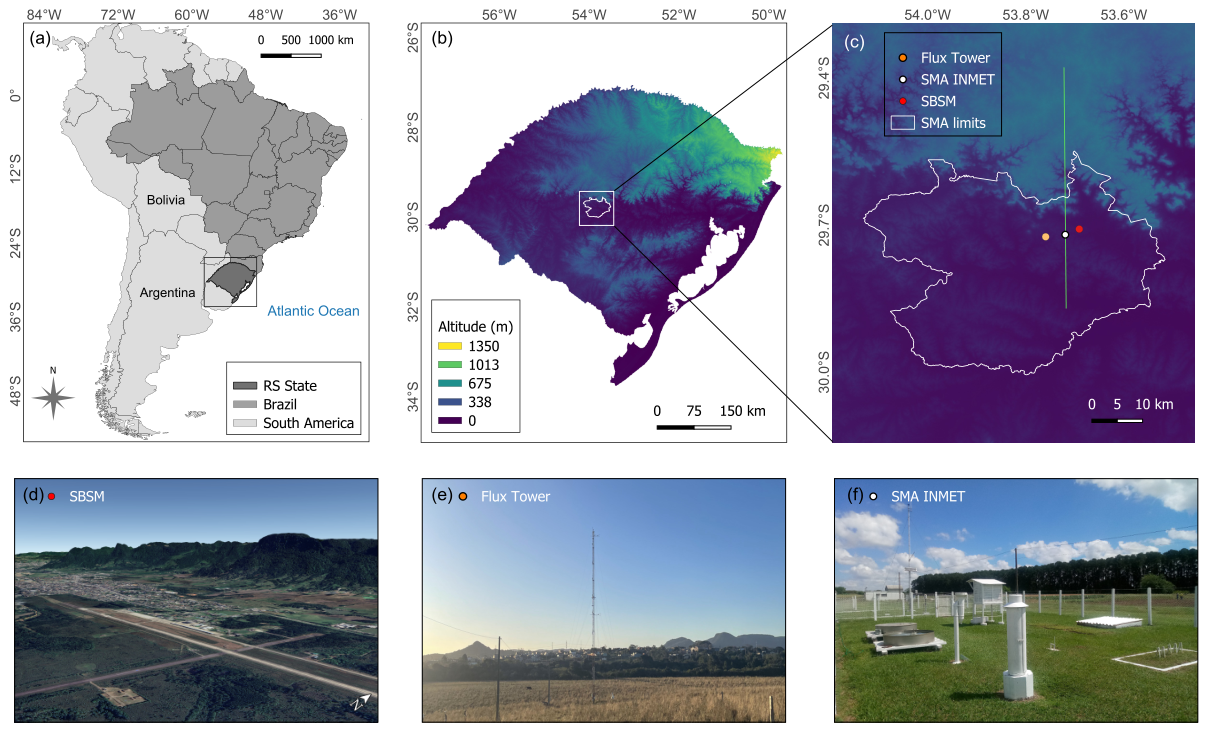
The study area is located in southern Brazil, with a specific focus on the central region of the RS state (Figure 1). The regional climate is strongly influenced by midlatitude atmospheric circulation, including the frequent passage of frontal systems and the intrusion of cold air masses originating from higher latitudes [16,17,18]. During winter, these cold air incursions can cause significant temperature drops, sometimes resulting in frost events [19,20] and, less frequently, snowfall [21]. In contrast, summer conditions are typically characterized by high air temperatures, often exceeding 35 °C. The climatological normals for August indicate a mean air temperature of 15.4 °C, a prevailing wind direction of 156° (south–southeast) with a mean wind speed of 2.1 m s⁻¹ and an air pressure of 1018 hPa. These climatological conditions provide the baseline atmospheric state against which the anomalous characteristics of the VNOR event are evaluated.

2.2. Observational and Reanalysis Data

The analysis is based on a comprehensive dataset consisting of observations from AWS, Meteorological Aerodrome Reports (METAR), radiosonde measurements, flux tower, and reanalysis data. These datasets provide complementary information on the main atmospheric and surface conditions on multiple spatial and temporal scales. A brief description of each dataset is provided below.

• To characterize the temporal evolution of the VNOR event on the surface, hourly observations from an AWS operated by the Brazilian National Institute of Meteorology (INMET; https://tempo.inmet.gov.br/; accessed on 10 March 2026) in Santa Maria (SMA), located in the central depression region (Figure 1c,f), were analyzed. Wind speed and direction are measured at 10 m, while air temperature and atmospheric pressure are measured at 2 m.
• METAR observations were used to complement gaps in wind speed and direction measurements. The data were obtained from the surface meteorological station located at Santa Maria Air Force Base (SBSM). Wind speed and direction at 10 m and air temperature at 2 m were used in the analysis. METAR reports are issued routinely at hourly intervals, and special reports (SPECI) are generated when significant meteorological changes occur. Data were accessed through the Brazilian Aeronautical Meteorology Network (REDEMET; https://www.redemet.aer.mil.br/; accessed on 10 March 2026).
• Atmospheric turbulence was analyzed using high-frequency observations from a 30 m flux tower located at the experimental site of the Universidade Federal de Santa Maria (UFSM; ${29}^{\circ }{43}^{\prime }27.{502}^{″}$ S, ${53}^{\circ }{45}^{\prime }36.{097}^{″}$ W). The site is located approximately 4 $\mathrm{k}$$\mathrm{m}$ south of the topographic slope (Figure 1c,e). Turbulent measurements of the three-dimensional wind velocity components (u, v, w) and sonic temperature were obtained using sonic anemometers installed at multiple vertical levels (1.5 to 30.0 m above ground level), with a sampling frequency of 10 $\mathrm{Hz}$. Here, turbulent quantities calculated at 11 m were used for comparison with the WRF simulations. Although turbulent fluxes were calculated at 11 m, both the observations and the WRF outputs are representative of the surface layer and are therefore expected to capture similar characteristics of the turbulent flow.
• To evaluate the vertical atmospheric patterns, high-resolution radiosonde observations collected twice daily at 0000 UTC (2100 LST; local standard time, UTC−3) and 1200 UTC (0900 LST) at SBSM were used. The SBSM station is located approximately 6 $\mathrm{k}$$\mathrm{m}$ east-northeast of the flux tower.
• ERA5 reanalysis data from the European Centre for Medium-Range Weather Forecasts (ECMWF) [22] were used to provide the initial and boundary conditions for the WRF simulations. Atmospheric fields are available on 37 pressure levels, ranging from 1000 hPa to 1 hPa, along with four soil layers representing subsurface conditions. The ERA5 data are provided at a horizontal spatial resolution of 0.25° × 0.25°.

2.3. Model Experiments

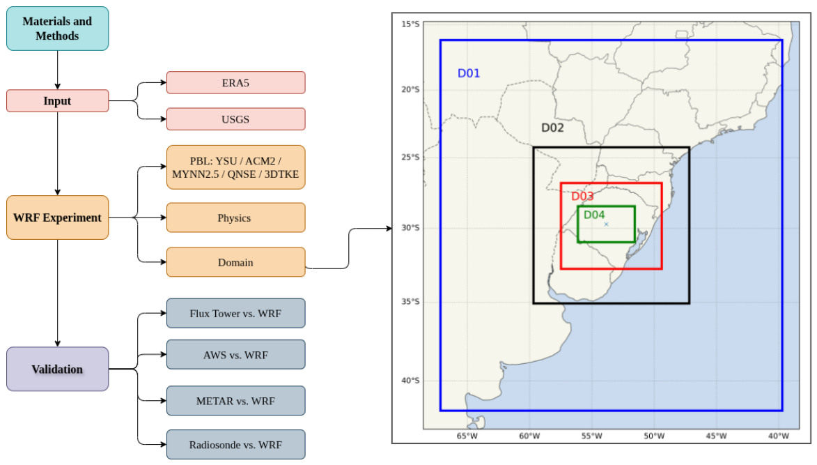
Figure 2 presents a schematic representation of the modeling framework adopted. The diagram presents the input datasets (ERA5 reanalysis and United States Geological Survey (USGS) data), the WRF model configuration (domains, physical parameterizations, and PBL schemes), and the validation strategy. Model performance is evaluated against independent observations (Section 2.2), enabling an assessment of the simulation of the VNOR event.

In this study, WRF-ARW version 4.5.2 was used. Initial and boundary conditions were obtained from the ERA5 reanalysis dataset, updated at 6-h intervals. Topography and soil characteristics were derived from the USGS dataset, with a horizontal spatial resolution of approximately 1 $\mathrm{k}$$\mathrm{m}$. To simulate the region of interest, four two-way nested domains were configured with horizontal grid spacings of 27 $\mathrm{k}$$\mathrm{m}$, 9 $\mathrm{k}$$\mathrm{m}$, 3 $\mathrm{k}$$\mathrm{m}$, and 1 $\mathrm{k}$$\mathrm{m}$, corresponding to domains D01, D02, D03, and D04, respectively. Following the configuration described by Duine et al. [6], the model was set up with 60 vertical levels, including 19 sigma levels within the lowest 1 $\mathrm{k}$$\mathrm{m}$ to enhance the representation of boundary-layer processes. However, a larger number of vertical levels and a different vertical spacing were adopted compared to Duine et al. [6]. Previous studies have demonstrated that finer vertical grid spacing is a key factor for accurately simulating low-level jets in the WRF model [23]. Model outputs were saved at 30 $\min$ intervals for the innermost domain (D04), which encompasses the study region and is centered at ${29}^{\circ }{48}^{\prime }36.0^{″}$ S, ${53}^{\circ }{47}^{\prime }02.5^{″}$ W. This domain includes the city of SMA and the surrounding terrain.

All simulations were initialized at 1200 UTC (0900 LST) on 18 August 2021, approximately 27 h before the onset of the VNOR event. The simulations were integrated until 1200 UTC (0900 LST) on 20 August 2021, resulting in a total simulation period of 48 h, encompassing the pre-event, event, and post-event atmospheric conditions.

2.4. Physics Parameterizations

For the physical parameterizations, the Thompson microphysics scheme [24] was used to represent cloud microphysical processes. Longwave and shortwave radiation were parameterized using the Rapid Radiative Transfer Model for General Circulation Models (RRTMG) [25]. Cumulus convection was represented using the modified Tiedtke scheme [6,26,27] in the outer domains (D01 and D02). In the inner domains (D03 and D04), with higher spatial resolutions, convection was treated explicitly. Land–atmosphere interactions were represented using the Noah Land Surface Model (Noah LSM) [28,29,30], which was kept fixed across all simulations. This scheme is widely used and has demonstrated robust performance in representing surface energy balance, soil thermodynamics, and land–atmosphere exchanges, including over complex terrain [6,31,32,33].

Given the fundamental role of the PBL in governing turbulence structure and momentum transport during downslope windstorm events, different PBL parameterization schemes were evaluated. The experimental design followed the methodology described by Duine et al. [6]. Specifically, the following PBL schemes were tested:

• Yonsei University (YSU);
• Asymmetric Convective Model Version 2 (ACM2);
• Mellor–Yamada–Nakanishi–Niino Level 2.5 (MYNN2.5);
• Quasi-Normal Scale Elimination (QNSE);
• Three-Dimensional Scale-Adaptive Turbulent Kinetic Energy (3DTKE).

The PBL parameterizations were selected based on previous results reported in the literature (e.g., [5,6,23], among others). The selection focused on the ability of each scheme to represent low-level jets, since their formation and intensification are frequent during VNOR episodes. Additional criteria included differences in closure level following the classification of Mellor and Yamada [34], the treatment of turbulence as local, nonlocal, or hybrid, and whether the parameterization follows a one-dimensional or three-dimensional approach.

The YSU [35] and ACM2 [36] schemes are classified as level-1 closure schemes. These schemes solve prognostic equations only for the mean state variables (e.g., wind components, temperature, and humidity), while turbulent fluxes are parameterized diagnostically. Consequently, no additional prognostic equations are solved to explicitly represent turbulent effects on the mean flow [37]. The YSU scheme is a nonlocal first-order closure in which turbulent fluxes are estimated using velocity scales and the PBL height, diagnosed through a critical Richardson number. The formulation includes a counter-gradient term to account for the contribution of large-scale eddies to the total flux, as well as an entrainment flux at the inversion layer. Both contributions are estimated through empirical relationships [35]. In the ACM2 scheme, turbulent mixing is represented by a combination of local (eddy-diffusivity) and nonlocal (mass-flux) components through a weighting factor. When this factor approaches zero, the scheme reduces to a purely local eddy-diffusion formulation. The nonlocal mass-flux component is active primarily under convective conditions, when buoyant eddies have characteristic scales larger than the vertical grid spacing [36].

The MYNN2.5 [38], QNSE [39], and 3DTKE [40] schemes are classified as level-2.5 closures. In these parameterizations, turbulent kinetic energy (TKE) is predicted through a prognostic equation, and eddy diffusivities are formulated as functions of TKE and a mixing length. Turbulent fluxes are computed based on local gradients of the mean variables. A key distinction among these schemes lies in their empirical formulations of mixing length scales and stability functions. The MYNN2.5 scheme incorporates an eddy-diffusivity mass-flux framework, in which local turbulent transport is represented by eddy diffusivity, while nonlocal transport associated with organized updrafts is represented by a mass-flux component [38]. The 3DTKE scheme introduces scale-aware behavior to ensure a smooth transition between mesoscale and large-eddy simulation (LES) regimes within the gray zone. This is achieved through blending functions that modulate the relative contributions of resolved and subgrid-scale turbulence as a function of grid spacing. In this approach, turbulent fluxes and mixing lengths are obtained by blending local and nonlocal, LES and mesoscale components using resolution-dependent weighting functions [40]. A major distinction of the 3DTKE scheme compared to the others is that horizontal turbulent fluxes are explicitly parameterized using a two-dimensional Smagorinsky-type first-order closure based on the resolved horizontal velocity deformation [40]. In contrast, the MYNN2.5, YSU, ACM2, and QNSE schemes adopt a one-dimensional column framework and represent turbulent transport and mixing processes exclusively in the vertical direction.

2.5. Evaluation Metrics

For continuous variables, statistical metrics can provide important information about model performance. Classic metrics such as standard deviation ($\sigma$), Pearson’s correlation coefficient (R), and root mean square error (RMSE) provide an overall assessment of variability, linear relationship, and accuracy between simulated and observed data [41]. These statistical metrics can be displayed using a Taylor Diagram, which is a polar plot that represents these three metrics in a single figure, with intercomparison between observed data and different simulations. Bias was additionally used to quantify the systematic overestimation or underestimation of the simulations relative to observations.

3. Results

3.1. Surface Observations Comparison

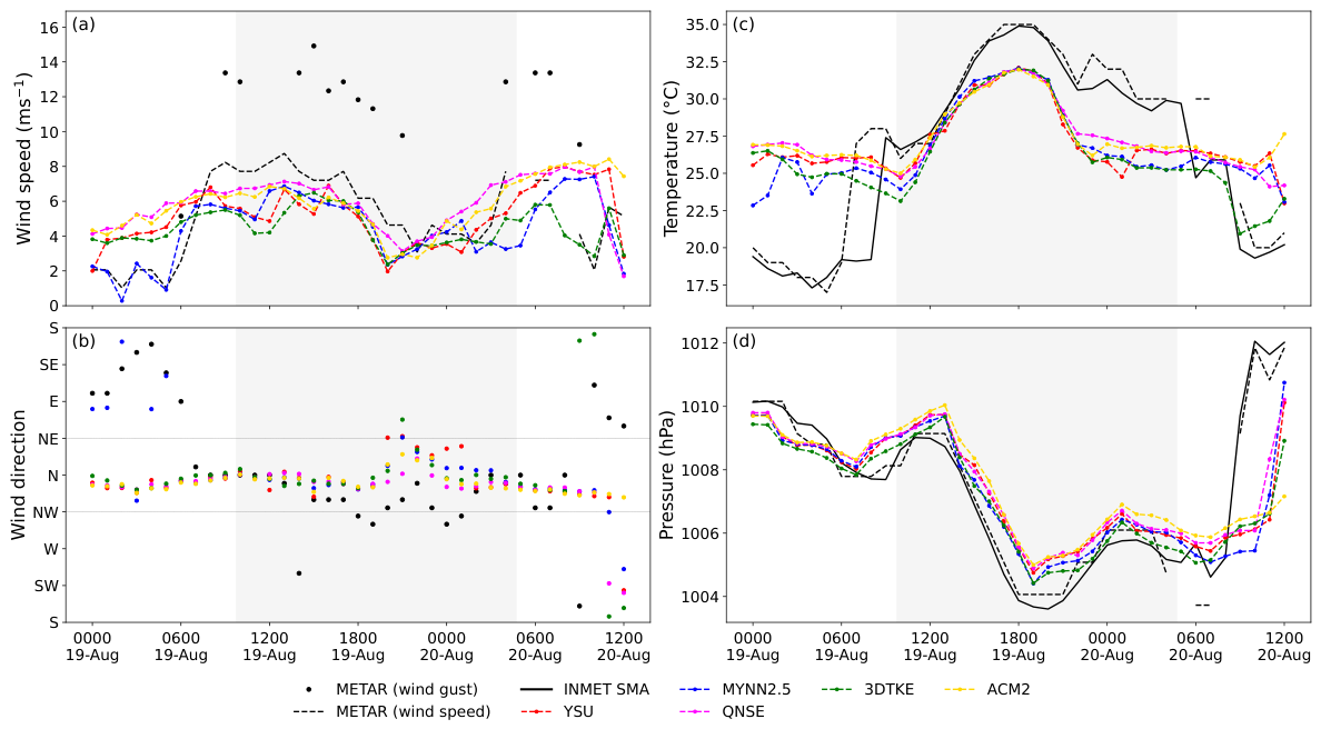
Figure 3 presents a comparison between AWS and METAR observations, and WRF simulations using different PBL parameterization schemes (YSU, MYNN2.5, QNSE, 3DTKE, and ACM2).

The observed wind speed (Figure 3a) remained weak during the early hours of 19 August, with values below 2.5 m s⁻¹ until approximately 0500 UTC. From 0600 UTC onward, a sharp increase marked the onset of the VNOR event. Among the simulations, MYNN2.5 best captures the low wind conditions before the VNOR onset at the surface, as well as the timing of this transition, although the magnitude of the intensification is underestimated. Wind speed peaks near 1200 UTC, exceeding 7.5 m s⁻¹ in the observations. However, all parameterizations underestimate the observed wind maximum. Until approximately 2100 UTC on 19 August, the simulations consistently underestimated the wind intensity. During the final stage of the event (0300–0600 UTC on 20 August), secondary wind intensification is observed and reasonably captured by the simulations.

Wind direction (Figure 3b) exhibits a clear shift toward the northern quadrant between 0600 and 0700 UTC on 19 August, defining the VNOR onset. MYNN2.5 reproduces this transition more realistically, capturing the preceding easterly flow and the subsequent shift to northerly winds. In contrast, the other parameterizations anticipate the directional change, indicating northerly winds before the observed transition (0500 UTC). Throughout most of the event, MYNN2.5 maintains predominantly northerly flow consistent with observations. Conversely, ACM2 and YSU show reduced skill, maintaining northerly winds even after the observed directional shift at the end of the event.

Air temperature (Figure 3c) increases rapidly following the wind intensification at 0600 UTC on 19 August, reaching values close to 35 °C around 1800 UTC. The abrupt warming characterizing the onset of VNOR is smoothed across all simulations. Moreover, simulations underestimate the observed temperature peak and tend to overestimate temperatures before the VNOR onset. The underestimation of wind speed was also identified by Duine et al. [6] during Sundowner wind events, regardless of the PBL scheme and land surface model configuration, suggesting a difficulty for WRF in reproducing downslope windstorms over complex terrain. One possible explanation for this behavior may be the terrain representation itself [42,43], as the smoothing of topography associated with limited horizontal resolution may weaken slope features and reduce the model’s ability to simulate local terrain-induced wind patterns.

Sea level pressure (Figure 3d) shows a gradual decrease throughout 19 August, reaching a minimum near 1800 UTC. This evolution is consistently reproduced by all simulations, which capture both the timing and magnitude of the pressure drop associated with the event.

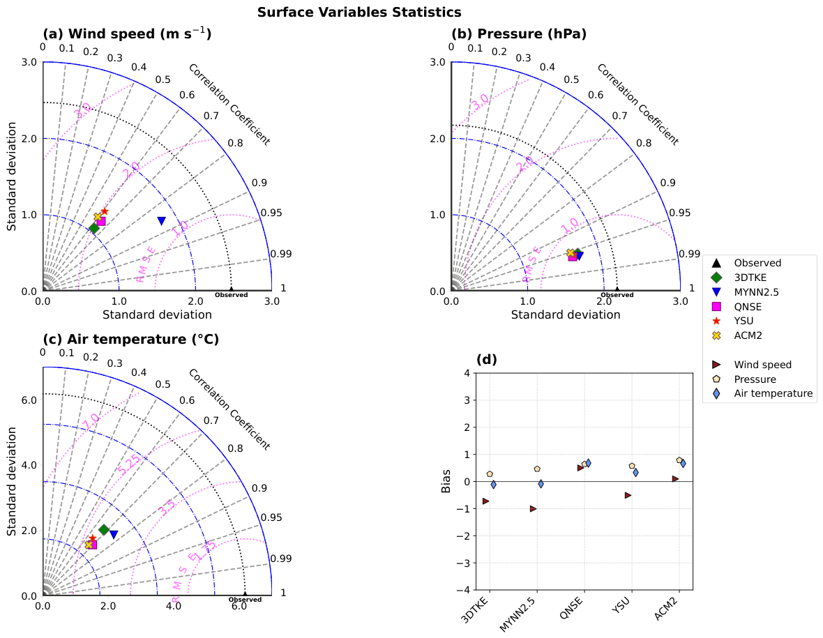
The Taylor diagrams (Figure 4a–c) summarize the statistical performance of the PBL schemes for near-surface variables before and during the VNOR event. For wind speed (Figure 4a), MYNN2.5 exhibits superior skill among the PBL schemes, presenting the highest correlation (R ≈ 0.85) and the lowest RMSE (close to 1 m s⁻¹) compared with the observations, indicating improved representation of both variability and temporal evolution of the wind speed. For pressure (Figure 4b), all schemes display very high R values. Differences among the PBL parameterizations are small. For air temperature (Figure 4c), MYNN2.5 again demonstrates the highest R and lowest RMSE values among the PBL schemes. The bias (Figure 4d) analysis complements these findings. MYNN2.5 and 3DTKE slightly underestimate wind speed but maintain near-zero bias for temperature. Surface pressure biases remain small across all schemes. Overall, for the analyzed VNOR case, MYNN2.5 provides the most consistent and robust statistical performance among the evaluated PBL schemes, indicating improved representation of near-surface conditions associated with the VNOR.

3.2. Radiosoundings Profiles Comparison

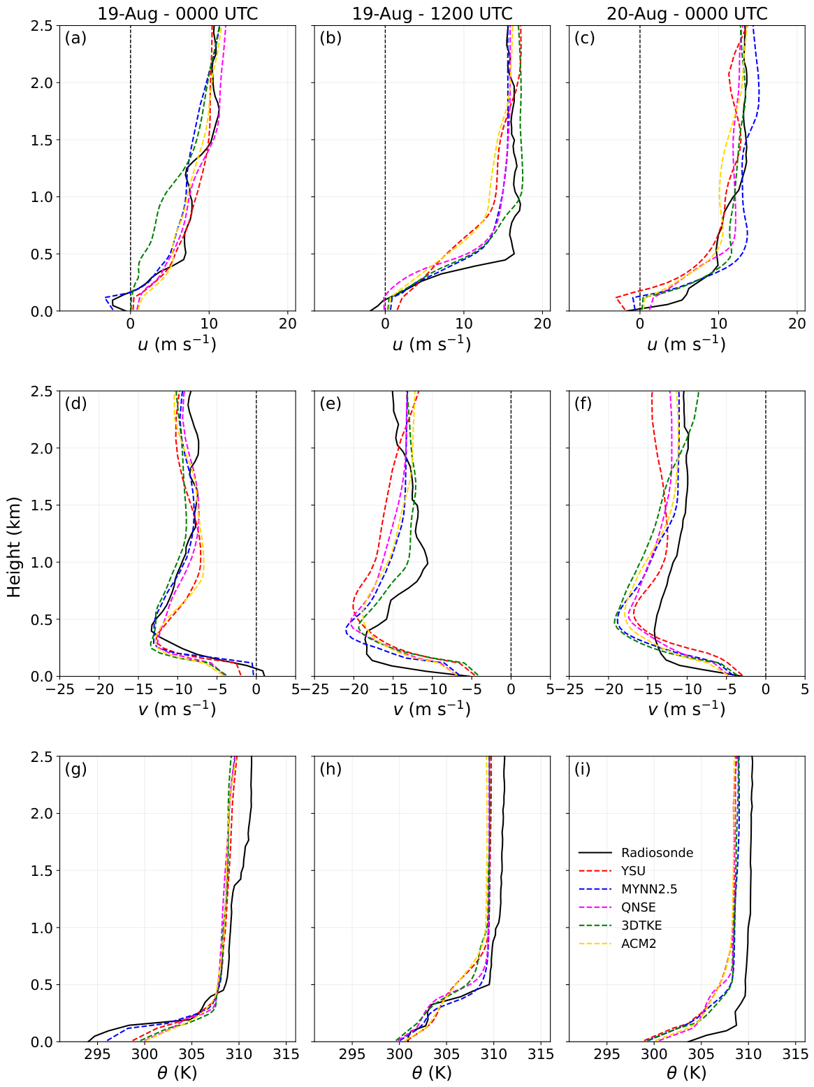
Figure 5 presents the vertical profiles of the zonal u and meridional v wind velocity components, and potential temperature ($\theta$), before and during the VNOR event.

For u, the 0000 UTC profile on 19 August (Figure 5a) shows weak and slightly negative values near the surface, transitioning to positive values aloft. All simulations reproduce the general vertical structure, with MYNN2.5 providing the closest agreement in the lowest levels. Among the schemes, 3DTKE presents the largest deviation from the observed structure. At 1200 UTC on 19 August (Figure 5b), a clear intensification of u is observed around 0.5 km, associated with the development of the low-level jet during VNOR. This feature is captured by all simulations, although the magnitude is underestimated. At 0000 UTC on 20 August (Figure 5c), u remains positive but weaker than at 1200 UTC. Most simulations reproduce the overall structure, though they tend to slightly overestimate wind speed near 0.5 km.

For v, the 0000 UTC profile on 19 August (Figure 5d), prior to surface VNOR onset, shows weak winds near the surface, a maximum around 0.5 km, and decreasing magnitudes aloft. All simulations capture this vertical pattern. MYNN2.5 shows the best agreement near the surface and realistically represents the intensity and height of the observed jet core. At 1200 UTC (Figure 5e), with VNOR fully developed, the observed profile exhibits a strong northerly jet core of approximately −18 m s⁻¹. All simulations overestimate both the height and intensity of this core. Near-surface values are generally well reproduced by MYNN2.5. At 0000 UTC on 20 August (Figure 5f), during the decay phase of VNOR, simulations continue to maintain an overly intense jet core compared to observations, with MYNN2.5 and 3DTKE producing values close to −20 m s⁻¹. This indicates a delayed weakening of the jet in the model configurations.

The $\theta$ profiles (Figure 5g–i) further illustrate the evolution of the PBL vertical structure during VNOR. At 0000 UTC on 19 August (Figure 5g), $\theta$ increases with height up to approximately 0.5 km and becomes nearly neutral above, characterizing a very SBL. MYNN2.5 most accurately reproduces this curvature and stratification. The other schemes exhibit weaker gradients and reduced curvature. At 1200 UTC on 19 August (Figure 5h), the observed profile indicates erosion of the SBL near the surface and progressive homogenization up to approximately 400 m. This vertical structure is reproduced by all simulations, with MYNN2.5 showing the best overall agreement with the observations. At 0000 UTC on 20 August (Figure 5i), the profile indicates reestablishment of an SBL, though with less pronounced curvature than on the previous night. All simulations underestimate the magnitude of the observed temperature gradient but reproduce its vertical variation.

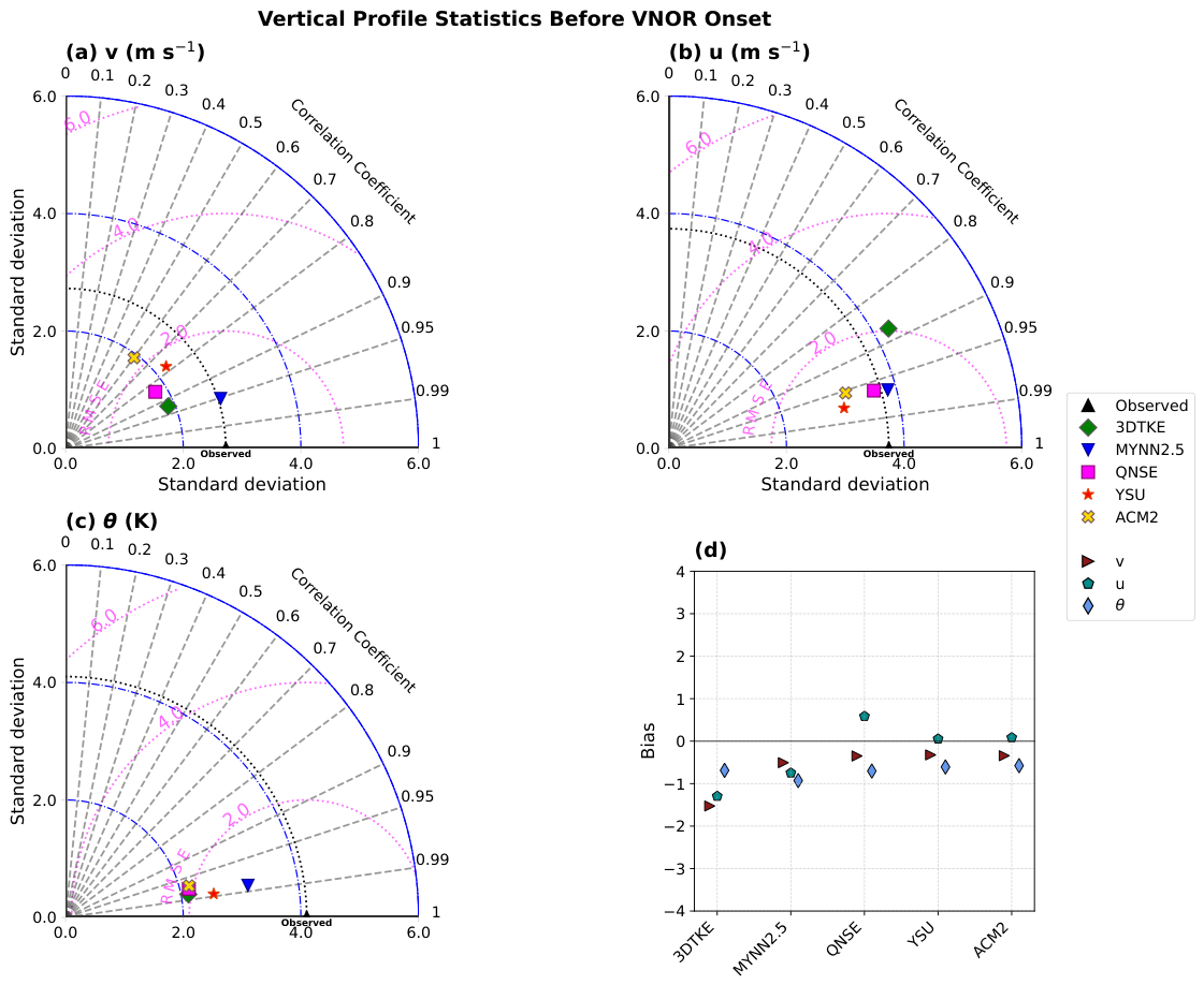
The Taylor diagrams for the vertical profiles (Figure 6 and Figure 7) provide an integrated assessment of the PBL schemes before and during the VNOR. Before the onset of VNOR, MYNN2.5 demonstrates superior performance for the v wind component (Figure 6a), exhibiting the highest R (0.95), the lowest RMSE, and a standard deviation nearly identical to the observed profile. This result indicates that MYNN2.5 represents the vertical structure well of the nocturnal lee low-level jet and the cross-barrier flow associated with the preconditioning phase of the VNOR event. For the u wind component (Figure 6b), MYNN2.5, QNSE, and YSU show similarly high correlation, with YSU presenting the lowest RMSE. For $\theta$ (Figure 6c), MYNN2.5 and YSU provide the lowest RMSE and high R, while slightly underestimating the observed variability. In terms of the bias distribution (Figure 6d), YSU and ACM2 showed similar low absolute differences compared to the vertical profiles observed. Overall, before the VNOR onset, MYNN2.5 exhibits the most consistent performance overall, indicating that it better reproduces the confined SBL.

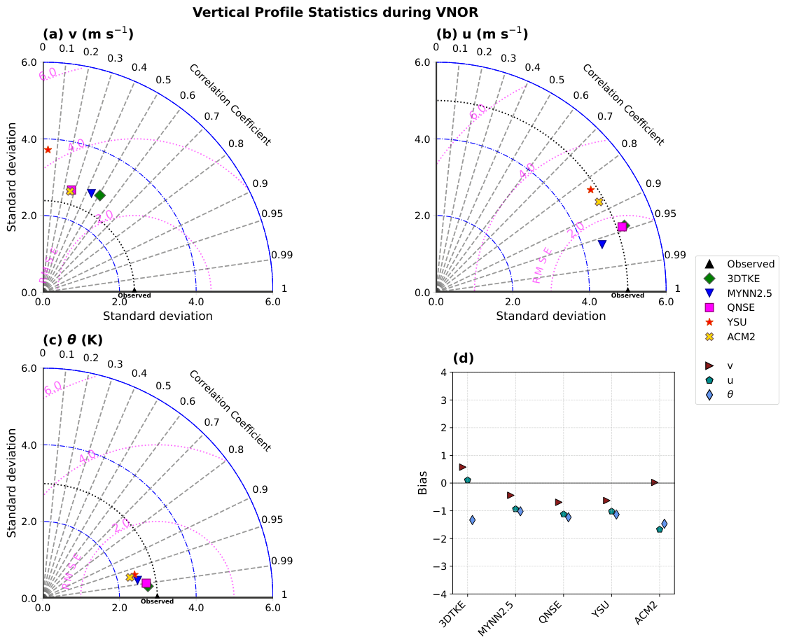
During the VNOR event (Figure 7), the skill of the model varies depending on the variable. For the v wind component (Figure 7a), all PBL schemes exhibit reduced agreement relative to the pre-event period. MYNN2.5 and 3DTKE tend to present the best statistical performance. For the u wind component (Figure 7b), MYNN2.5 maintains the highest correlation among the PBL schemes and one of the lowest RMSE values. For $\theta$ (Figure 7c), QNSE and 3DTKE show slightly better correlations and variability closer to the observations, similar to ERA performance, while the other PBL schemes exhibit similar performance. The bias analysis (Figure 7d) reinforces these findings, showing that, in general, the absolute differences are lowest for the MYNN2.5, QNSE, and YSU schemes.

Taken together, the results indicate that MYNN2.5 provides the most robust and consistent representation of the vertical boundary-layer structure, particularly before VNOR. It also maintains competitive performance during the development and mature stage of the VNOR event.

3.3. Comparison with Turbulence Observations

This section evaluates the performance of the WRF PBL schemes in reproducing the temporal evolution of turbulent variables before and during the VNOR event.

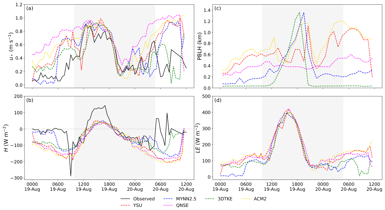
The friction velocity (u∗; Figure 8a) exhibits weak values between 0000 and 0600 UTC on 19 August, indicating suppressed turbulence under stable stratification and weak winds. After 0600 UTC, u∗ increases, coinciding with the wind intensification (Figure 3a) and marking the onset of VNOR. Around 1200 UTC, observed u∗ exceeds 0.8 m s⁻¹, reflecting strong mechanically driven turbulence associated with enhanced vertical shear. Among the simulations, MYNN2.5 most accurately reproduces both the pre-VNOR regime and the transition to intensified turbulence, capturing the timing and magnitude of the u∗ peak. 3DTKE represents the general trend but overestimates turbulence prior to VNOR onset, suggesting excessive mixing under stable conditions. After 1800 UTC, u∗ decreases progressively, reaching approximately 0.2 m s⁻¹ near 2300 UTC, following the weakening of VNOR and the reestablishment of the SBL. A secondary increase near the event demise is also observed, and the simulations diverge in their representation.

The sensible heat flux (H; Figure 8b) remains slightly negative and close to zero until 0600 UTC on 19 August, consistent with SBL conditions. MYNN2.5 provides the most realistic representation during this period. After 0600 UTC, a pronounced negative flux precedes a transition to positive values, marking the arrival of VNOR, a behavior previously documented by Stefanello et al. [11]. Subsequently, H increases, exceeding 100 W m⁻² between 13 and 1700 UTC. None of the WRF simulations reproduces this observed magnitude. The consistent underestimation of H among all simulations suggests a systematic deficiency beyond the PBL parameterizations themselves. In fact, the soil heat flux simulated by the model reaches values close to 150 W m⁻² during the daytime, substantially higher than those typically observed at the site and during VNOR episodes [11,44,45]. Although a detailed investigation of this issue is beyond the scope of the present study, this behavior may indicate deficiencies associated with land surface parameters, soil moisture initialization, or the Noah LSM configuration. After 1800 UTC, simulations better follow the observed variability.

The latent heat flux ($LE$; Figure 8c), available only from WRF simulations, remains weak until 0600 UTC. Thereafter, $LE$ increases markedly, reaching a maximum near 1500 UTC. During this period, all WRF simulations converge to values exceeding 400 W m⁻². The elevated $LE$ during the most intense phase of VNOR indicates enhanced evaporation driven by warm and dry northerly winds, consistent with Stefanello et al. [11]. After the VNOR peak, $LE$ decreases, remaining below 200 W m⁻² after 2000 UTC.

The evolution of the PBL height (PBLH; Figure 8d) further illustrates the transition between stable and convective conditions. During the nighttime preceding VNOR onset, a shallow SBL confined by local topography is established. QNSE and MYNN2.5 best reproduce this shallow SBL, whereas other schemes either overestimate PBLH or simulate an unrealistically thin layer. QNSE maintains an almost constant PBLH throughout the event, indicating limited responsiveness to changing stability conditions. In contrast, 3DTKE, MYNN2.5, and ACM2 capture the marked increase in PBLH after 1800 UTC, associated with daytime heating and intensified turbulent mixing. Overall, MYNN2.5 provides the most realistic temporal evolution, representing both the shallow SBL preceding VNOR and the development of a convective boundary layer exceeding 1 km after 1800 UTC. This behavior reinforces its superior ability to simulate the PBL turbulence flow. While Figure 8d illustrates the evolution of PBLH during the VNOR, a direct comparison among schemes should be interpreted with caution, since PBLH is diagnosed and used differently depending on the closure formulation. YSU and ACM2 diagnose PBLH using Richardson-number threshold approaches and directly employ this quantity to determine the vertical extent and intensity of turbulent mixing. In contrast, MYNN2.5, QNSE, and 3DTKE are based on local TKE closures, where turbulent transport is primarily governed by local turbulence and atmospheric stability. Consequently, differences in diagnosed PBLH reflect not only varying boundary-layer depths but also distinct turbulence closure assumptions.

The comparison with flux tower observations provides additional insight into the representation of turbulent processes by the different PBL schemes. For u∗, 3DTKE and MYNN2.5 exhibit the best statistical performance, while for H, the performance of all schemes is more limited. MYNN2.5 and ACM2 present the best statistical performance. However, all schemes underestimate the observed variability and magnitude of the flux. The differences in turbulence closure assumptions may also help explain why, although 3DTKE generally reproduces the temporal evolution of turbulence variables and PBL development (Figure 5, Figure 6, Figure 7 and Figure 8), its performance is comparable to, rather than systematically better than, that of the conventional 1D schemes. Previous studies (e.g., [46]) demonstrate that the scale-aware partitioning adopted by 3DTKE may reduce subgrid TKE more aggressively than the corresponding increase in resolved TKE, limiting gains in total turbulence representation. Furthermore, despite its 3D structural formulation, the scheme still relies on similarity functions similar to those utilized by conventional 1D schemes. Since turbulence remains only partially resolved at a 1 km resolution, conventional 1D schemes may still perform competitively under these conditions. This behavior is particularly relevant during downslope windstorm events, where the representation of turbulent momentum exchange and PBL development strongly controls near-surface wind intensity.

3.4. Cross Sections Patterns

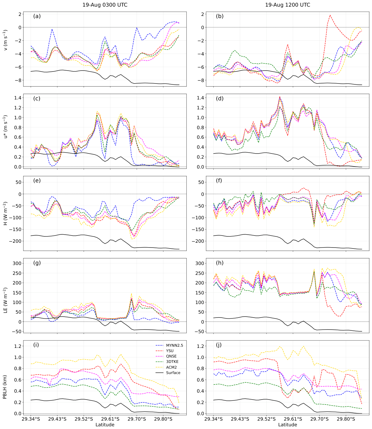
Simulations indicate that prior to the surface onset of VNOR at SMA (0300 UTC on 19 August; Figure 9a,c,e,g,i), v wind component and u∗ intensify at the topographic slope. Immediately south of the slope, within the central depression, winds remain weak, and u∗ is low, indicating suppressed turbulence under stable conditions. The turbulent fluxes follow a similar intensification pattern. H remains negative across the domain, consistent with stable nocturnal conditions. H and $LE$ show enhancement near the slope. All PBL schemes simulate a deeper SBL north of the slope, where turbulent mixing is more intense, whereas a shallower SBL is observed confined in the valley.

At 1200 UTC on 19 August (Figure 9b,d,f,h,j), during the VNOR, the v wind component and u∗ are markedly enhanced along the slope and immediately southward. This pattern reflects strong mechanically driven turbulence promoted by downslope flow acceleration. Both H and $LE$ intensify over the slope and immediately south of it. At this stage, a pronounced increase in PBLH is simulated south of the slope, associated with stronger turbulent mixing and erosion of the nocturnal boundary layer. The spatial correspondence between enhanced wind speed, increased u∗, and elevated PBLH suggests that terrain-induced flow acceleration plays a key role in modulating PBL structure during VNOR.

The PBLH observed before and during the VNOR in Figure 9 indicates generally lower PBLH for the local TKE-based schemes (MYNN2.5, QNSE, and 3DTKE) than for the nonlocal and hybrid schemes (YSU and ACM2), consistent with results previously reported for Sundowner simulations by Duine et al. [6]. The spatial variability of u∗, H, and $LE$ (Figure 9) among PBL schemes is also likely attributable to differences in the representation of turbulent mixing. In general, the local TKE-based schemes simulate lower PBLH and weaker turbulent fluxes. In contrast, the nonlocal and hybrid schemes tend to produce larger turbulent fluxes and deeper PBLH. South of the slope, the local TKE-based schemes generally exhibit more similar spatial patterns, while the nonlocal and hybrid schemes tend to deviate, simulating different magnitudes of PBLH and turbulent fluxes. These differences may suggest distinct representations of turbulent coupling among the PBL schemes before and during the VNOR event.

4. Summary and Conclusions

This study investigated the sensitivity of the WRF model to different PBL parameterization schemes in simulating a typical VNOR windstorm over modest terrain in southern Brazil. Five PBL schemes were evaluated for their ability to reproduce the key features of a VNOR event that occurred between 19 and 20 August 2021. Model simulations were compared against multiple observational datasets, including AWS measurements, radiosonde profiles, flux tower observations, and METAR reports. This comprehensive evaluation provides new insight into the capability of different PBL schemes to represent the temporal evolution, vertical structure, and spatial variability of terrain-induced downslope windstorms.

During the nighttime period preceding VNOR onset, a strongly SBL confined by local topography was observed. Above this layer, a nocturnal low-level jet developed, with maximum wind speeds occurring near the terrain slope. Among the evaluated schemes, MYNN2.5 provided the most accurate representation of the pre-VNOR atmospheric structure, including near-surface wind speed and wind direction. This scheme also better captured the initial phase of VNOR, characterized by the progressive erosion of the leeward SBL. However, MYNN2.5, as well as the other parameterizations, showed limitations in reproducing the minimum air temperature and its temporal evolution.

During the VNOR event, the low-level jet intensified relative to pre-event conditions, and strong northerly winds promoted rapid warming and drying of the PBL, associated with enhanced turbulent mixing. MYNN2.5 again provided the most accurate representation of the vertical profiles of potential temperature and wind components. Despite their overall good performance, all simulations underestimated the maximum surface air temperature during VNOR. In contrast, the temporal evolution of the surface pressure field was well reproduced by all parameterizations throughout the pre-event, event, and post-event periods.

VNOR was also characterized by a marked intensification of turbulent activity, with an abrupt transition from a weakly turbulent regime associated with a strongly SBL to a fully turbulent regime following its onset. MYNN2.5 most realistically reproduced this transition, particularly in its representation of friction velocity evolution. Nevertheless, even the best-performing configurations, including MYNN2.5, showed limitations in accurately simulating sensible heat flux.

The integrated statistical evaluation demonstrated that the MYNN2.5 provided the most accurate overall representation of VNOR conditions. MYNN2.5 were further evaluated in additional VNOR cases reported in [47,48], confirming the robustness and consistency of these results across different VNOR events. However, since in the present study the intercomparison among all PBL parameterization schemes was performed for a single VNOR case, the relative superiority of MYNN2.5 may still depend on the specific characteristics of the analyzed event.

The present findings provide a foundation for future high-resolution simulations aimed at improving the understanding of the physical mechanisms governing SBL erosion and the role of gravity waves and other dynamical forcing processes in the development and evolution of VNOR.

References

1. Stull, R.B. An Introduction to Boundary Layer Meteorology; Kluwer Academic Publishers: Dordrecht, The Netherlands, 1988. [Google Scholar]
2. Ito, J.; Niino, H.; Nakanishi, M.; Moeng, C.H. An extension of the Mellor–Yamada model to the terra incognita zone for dry convective mixed layers in the free convection regime. Bound.-Layer Meteorol. 2015, 157, 23–43. [Google Scholar] [CrossRef] [Scilit]
3. Dudhia, J. Challenges in sub-kilometer grid modeling of the convective planetary boundary layer. Meteorology 2022, 1, 402–413. [Google Scholar] [CrossRef] [Scilit]
4. Mahrt, L. Stably stratified atmospheric boundary layers. Annu. Rev. Fluid Mech. 2014, 46, 23–45. [Google Scholar] [CrossRef] [Scilit]
5. Maroneze, R.; Acevedo, O.C.; Costa, F.D.; Puhales, F.S.; Anabor, V.; Lemes, D.N., Jr.; Mortarini, L. How is the two-regime stable boundary layer reproduced by the different turbulence parametrizations in the weather research and forecasting model? Bound.-Layer Meteorol. 2021, 178, 383–413. [Google Scholar] [CrossRef] [Scilit]
6. Duine, G.J.; Jones, C.; Carvalho, L.M.; Fovell, R.G. Simulating Sundowner Winds in Coastal Santa Barbara: Model Validation and Sensitivity. Atmosphere 2019, 10, 155. [Google Scholar] [CrossRef] [Scilit]
7. Ma, Y.F.; Wang, Y.; Xian, T.; Tian, G.; Lu, C.; Mao, X.; Wang, L.P. Impact of PBL schemes on multiscale WRF modeling over complex terrain, Part I: Mesoscale simulations. Atmos. Res. 2024, 297, 107117. [Google Scholar] [CrossRef] [Scilit]
8. Matějka, M.; Řehoř, J.; Brázdil, R.; Štěpánek, P.; Zahradníček, P. Foehn warming mechanism and near-surface weather impact at the northern foreland of the Moravian-Silesian Beskids, Czech Republic. Theor. Appl. Climatol. 2025, 156, 145. [Google Scholar] [CrossRef] [Scilit]
9. Lee, Y.H.; Lim, H.J.; Lee, G. Planetary Boundary Layer Flow over Complex Terrain during a Cold Surge Event: A Case Study. Atmosphere 2024, 15, 153. [Google Scholar] [CrossRef] [Scilit]
10. Zhong, J.; Su, D.; Zheng, Z.; Kong, W.; Fang, P.; Mo, F. Evaluation of WRF Planetary Boundary Layer Parameterization Schemes for Dry Season Conditions over Complex Terrain in the Liangshan Prefecture, Southwestern China. Atmosphere 2026, 17, 53. [Google Scholar] [CrossRef] [Scilit]
11. Stefanello, M.B.; De Lima Nascimento, E.; Da Rosa, C.E.; Degrazia, G.; Mortarini, L.; Cava, D. A Micrometeorological Analysis of the Vento Norte Phenomenon in Southern Brazil. Bound.-Layer Meteorol. 2020, 176, 415–439. [Google Scholar] [CrossRef] [Scilit]
12. da Rosa, C.E.; Stefanello, M.; Facco, D.S.; Roberti, D.R.; Rossi, F.D.; Nascimento, E.d.L.; Degrazia, G.A. Regional-scale meteorological characteristics of the Vento Norte phenomenon observed in Southern Brazil. Environ. Fluid Mech. 2022, 22, 819–837. [Google Scholar] [CrossRef] [Scilit]
13. Rosa, C.E.D.; Stefanello, M.B.; Nascimento, E.D.L.; Rossi, F.D.; Roberti, D.R.; Degrazia, G.A. Meteorological Observations of the Vento Norte Phenomenon in the Central Region of Rio Grande do Sul. Rev. Bras. Meteorol. 2021, 36, 367–376. [Google Scholar] [CrossRef] [Scilit]
14. Stefanello, M.B.; Ewerling Da Rosa, C.; De Lima Nascimento, E.; Da Silva Rebelo, M.; Acevedo, O.C.; Carvalho, L.M.V.; Jones, C.; Degrazia, G. Gravity waves induced by a downslope windstorm in modest terrain: A case study. Q. J. R. Meteorol. Soc. 2025, 151, e5001. [Google Scholar] [CrossRef] [Scilit]
15. Arbage, M.C.A.; Degrazia, G.A.; Welter, G.S.; Roberti, D.R.; Acevedo, O.C.; de Moraes, O.L.L.; Ferraz, S.T.; Timm, A.U.; Moreira, V.S. Turbulent statistical characteristics associated to the north wind phenomenon in southern Brazil with application to turbulent diffusion. Phys. A Stat. Mech. Its Appl. 2008, 387, 4376–4386. [Google Scholar] [CrossRef] [Scilit]
16. Garreaud, R. Cold Air Incursions over Subtropical and Tropical South America: A Numerical Case Study. Mon. Weather Rev. 1999, 127, 2823–2853. [Google Scholar] [CrossRef] [Scilit]
17. Garreaud, R. Cold Air Incursions over Subtropical South America: Mean Structure and Dynamics. Mon. Weather Rev. 2000, 128, 2544–2559. [Google Scholar] [CrossRef] [Scilit]
18. Vera, C.S.; Vigliarolo, P.K. A Diagnostic Study of Cold-Air Outbreaks over South America. Mon. Weather Rev. 2000, 128, 3–24. [Google Scholar] [CrossRef] [Scilit]
19. Müller, G.V.; Berri, G.J. Atmospheric Circulation Associated with Persistent Generalized Frosts in Central-Southern South America. Mon. Weather Rev. 2007, 135, 1268–1289. [Google Scholar] [CrossRef] [Scilit]
20. Müller, G.V.; Berri, G.J. Atmospheric Circulation Associated with Extreme Generalized Frosts Persistence in Central-Southern South America. Clim. Dyn. 2012, 38, 837–857. [Google Scholar] [CrossRef] [Scilit]
21. Mintegui, J.M.; Puhales, F.S.; Boiaski, N.T.; Nascimento, E.D.L.; Anabor, V. Some Mean Atmospheric Characteristics for Snowfall Occurrences in Southern Brazil. Meteorol. Atmos. Phys. 2019, 131, 389–412. [Google Scholar] [CrossRef] [Scilit]
22. Hersbach, H.; Bell, B.; Berrisford, P.; Hirahara, S.; Horányi, A.; Muñoz-Sabater, J.; Nicolas, J.; Peubey, C.; Radu, R.; Schepers, D.; et al. The ERA5 global reanalysis. Q. J. R. Meteorol. Soc. 2020, 146, 1999–2049. [Google Scholar] [CrossRef] [Scilit]
23. Smith, E.N.; Gibbs, J.A.; Fedorovich, E.; Klein, P.M. WRF Model study of the Great Plains low-level jet: Effects of grid spacing and boundary layer parameterization. J. Appl. Meteorol. Climatol. 2018, 57, 2375–2397. [Google Scholar] [CrossRef] [Scilit]
24. Thompson, G.; Rasmussen, R.M.; Manning, K. Explicit Forecasts of Winter Precipitation Using an Improved Bulk Microphysics Scheme. Part I: Description and Sensitivity Analysis. Mon. Weather Rev. 2004, 132, 519–542. [Google Scholar] [CrossRef] [Scilit]
25. Iacono, M.J.; Delamere, J.S.; Mlawer, E.J.; Shephard, M.W.; Clough, S.A.; Collins, W.D. Radiative Forcing by Long-Lived Greenhouse Gases: Calculations with the AER Radiative Transfer Models. J. Geophys. Res. Atmos. 2008, 113, 2008JD009944. [Google Scholar] [CrossRef] [Scilit]
26. Tiedtke, M. A Comprehensive Mass Flux Scheme for Cumulus Parameterization in Large-Scale Models. Mon. Weather Rev. 1989, 117, 1779–1800. [Google Scholar] [CrossRef] [Scilit]
27. Zhang, C.; Wang, Y.; Hamilton, K. Improved Representation of Boundary Layer Clouds over the Southeast Pacific in ARW-WRF Using a Modified Tiedtke Cumulus Parameterization Scheme. Mon. Weather Rev. 2011, 139, 3489–3513. [Google Scholar] [CrossRef] [Scilit]
28. Niu, G.Y.; Yang, Z.L.; Mitchell, K.E.; Chen, F.; Ek, M.B.; Barlage, M.; Kumar, A.; Manning, K.; Niyogi, D.; Rosero, E.; et al. The community Noah land surface model with multiparameterization options (Noah-MP): 1. Model description and evaluation with local-scale measurements. J. Geophys. Res. 2011, 116, D12109. [Google Scholar] [CrossRef] [Scilit]
29. Yang, Z.L.; Niu, G.Y.; Mitchell, K.E.; Chen, F.; Ek, M.B.; Barlage, M.; Longuevergne, L.; Manning, K.; Niyogi, D.; Tewari, M.; et al. The community Noah land surface model with multiparameterization options (Noah-MP): 2. Evaluation over global river basins. J. Geophys. Res. 2011, 116, D12110. [Google Scholar] [CrossRef] [Scilit]
30. He, C.; Valayamkunnath, P.; Barlage, M.; Chen, F.; Gochis, D.; Cabell, R.; Schneider, T.; Rasmussen, R.; Niu, G.Y.; Yang, Z.L.; et al. The Community Noah-MP Land Surface Modeling System Technical Description Version 5.0; Technical Report; UCAR/NCAR: Boulder, CO, USA, 2023. [Google Scholar] [CrossRef]
31. Tewari, M.; Chen, F.; Wang, W.; Dudhia, J.; Lemone, M.A.; Mitchell, K.E.; Ek, M.; Gayno, G.; Wegiel, J.W.; Cuenca, R. Implementation and verification of the unified Noah land-surface model in the WRF model. In Proceedings of the 20th Conference on Weather Analysis and Forecasting/16th Conference on Numerical Weather Prediction; American Meteorological Society: Boston, MA, USA, 2004. [Google Scholar]
32. Hogue, T.S.; Bastidas, L.; Gupta, H.; Sorooshian, S.; Mitchell, K.; Emmerich, W. Evaluation and Transferability of the Noah Land Surface Model in Semiarid Environments. J. Hydrometeorol. 2005, 6, 68–84. [Google Scholar] [CrossRef] [Scilit]
33. Liu, X.; Cao, J.; Xin, D. Wind field numerical simulation in forested regions of complex terrain: A mesoscale study using WRF. J. Wind. Eng. Ind. Aerodyn. 2022, 222, 104915. [Google Scholar] [CrossRef] [Scilit]
34. Mellor, G.L.; Yamada, T. A hierarchy of turbulence closure models for planetary boundary layers. J. Atmos. Sci. 1974, 31, 1791–1806. [Google Scholar] [CrossRef] [Scilit]
35. Hong, S.Y.; Noh, Y.; Dudhia, J. A new vertical diffusion package with an explicit treatment of entrainment processes. Mon. Weather Rev. 2006, 134, 2318–2341. [Google Scholar] [CrossRef] [Scilit]
36. Pleim, J.E. A combined local and nonlocal closure model for the atmospheric boundary layer. Part I: Model description and testing. J. Appl. Meteorol. Climatol. 2007, 46, 1383–1395. [Google Scholar] [CrossRef] [Scilit]
37. Verma, S.; Panda, J.; Rath, S.S. Role of PBL and microphysical parameterizations during WRF simulated monsoonal heavy rainfall episodes over Mumbai. Pure Appl. Geophys. 2021, 178, 3673–3702. [Google Scholar] [CrossRef] [Scilit]
38. Olson, J.B.; Kenyon, J.S.; Angevine, W.; Brown, J.M.; Pagowski, M.; Sušelj, K. A Description of the MYNN-EDMF Scheme and the Coupling to Other Components in WRF–ARW; NOAA: Washington, DC, USA, 2019.
39. Skamarock, W.C.; Klemp, J.B.; Dudhia, J.; Gill, D.O.; Liu, Z.; Berner, J.; Wang, W.; Powers, J.G.; Duda, M.G.; Barker, D.M.; et al. A Description of the Advanced Research WRF Version 4; NCAR Tech. Note ncar/tn-556+ str; National Center for Atmospheric Research Boulder: Boulder, CO, USA, 2019; pp. 1–162. [Google Scholar]
40. Zhang, X.; Bao, J.W.; Chen, B.; Grell, E.D. A Three-Dimensional Scale-Adaptive Turbulent Kinetic Energy Scheme in the WRF-ARW Model. Mon. Weather Rev. 2018, 146, 2023–2045. [Google Scholar] [CrossRef] [Scilit]
41. Wilks, D.S. Statistical Methods in the Atmospheric Sciences; Academic Press: Cambridge, MA, USA, 2011; Volume 100. [Google Scholar]
42. Gómez-Navarro, J.J.; Raible, C.C.; Dierer, S. Sensitivity of the WRF model to PBL parametrisations and nesting techniques: Evaluation of wind storms over complex terrain. Geosci. Model Dev. 2015, 8, 3349–3363. [Google Scholar] [CrossRef] [Scilit]
43. Battisti, A.; Acevedo, O.C.; Costa, F.D.; Puhales, F.S.; Anabor, V.; Degrazia, G.A. Evaluation of Nocturnal Temperature Forecasts Provided by the Weather Research and Forecast Model for Different Stability Regimes and Terrain Characteristics. Bound.-Layer Meteorol. 2017, 162, 523–546. [Google Scholar] [CrossRef] [Scilit]
44. Zimmer, T.; de Arruda Souza, V.; Romio, L.C.; Buligon, L.; Veeck, G.P.; Stefanello, M.B.; Roberti, D.R. Estimation of soil thermal properties using conduction and conduction–convection heat transfer equations in the Brazilian Pampa biome. Agric. For. Meteorol. 2023, 338, 109517. [Google Scholar] [CrossRef] [Scilit]
45. Veeck, G.P.; de Arruda Souza, V.; Stefanello, M.B.; Mergen, A.; Bremm, T.; Zimmer, T.; Ruhoff, A.; Lyra, G.B.; Gonçalves, L.G.G.; Bresciani, C.; et al. Evapotranspiration partitioning and water-use efficiency in natural grasslands of the Brazilian Pampa biome. Agric. For. Meteorol. 2026, 384, 111162. [Google Scholar] [CrossRef] [Scilit]
46. Hope, A.P.; Lopez-Coto, I.; Hajny, K.; Tomlin, J.M.; Kaeser, R.; Stirm, B.; Karion, A.; Shepson, P.B. Analyzing “Gray Zone” Turbulent Kinetic Energy Predictions in the Boundary Layer from Three WRF PBL Schemes over New York City and Comparison with Aircraft Measurements. J. Appl. Meteorol. Climatol. 2024, 63, 125–142. [Google Scholar] [CrossRef] [Scilit]
47. Stefanello, M.; Lopes, M.M.; de Souza, E.C.; Rebelo, M.S.; Santos, D.C.; Zimmer, T.; da Rosa, C.E.; Santana, R.; da Silva, J.A.V.; da Rosa, H.V.B.; et al. An Overview of the “Vento Norte” Experiment (VNorEx): Observations of Downslope Windstorms over Modest Terrain in Southern Brazil. Adv. Atmos. Sci. 2026, 1861–9533. [Google Scholar] [CrossRef] [Scilit]
48. Nascimento, E.d.L.; Boiaski, N.T.; Ferraz, S.E.T.; Dal Piva, E.; Anabor, V.; Tatsch, J.D.; Puhales, F.S.; Stefanello, M.B.; Santos, D.C.; Lopes, M.M.; et al. From anomalous SST gradients in the Indian Ocean to floods and tornadoes in southern Brazil: The multi-scale nature of a historical precipitation event. Bull. Am. Meteorol. Soc. 2026, 107, E485–E500. [Google Scholar] [CrossRef] [Scilit]
Figure 1. Geographic setting and instrumentation position in the study area. (a) South America highlighting the state of Rio Grande do Sul (RS), Brazil; (b) topography of RS showing elevation gradients and the location of Santa Maria (SMA); (c) detailed view of the SMA, indicating the locations of the flux tower, the INMET AWS (SMA INMET), and Santa Maria Air Force Base (SBSM), along with the limits of the study area; (d) three-dimensional satellite-derived view illustrating topographic features near SBSM; (e) flux tower; and (f) the INMET AWS. The green line on (c) represents the location of horizontal cross sections.
Atmosphere 17 00550 g001
Figure 2. Overview of the methodological workflow and WRF model configuration used, including input datasets, model setup, and validation. The right panel shows the four nested WRF domains (D01–D04).
Atmosphere 17 00550 g002
Figure 3. Comparison of hourly observed data (INMET and METAR; black) and WRF model simulations (YSU, MYNN2.5, 3DTKE, QNSE, and ACM2) for the period from 0000 UTC on August 19 to 1200 UTC on 20 August 2021. The panels show: (a) wind speed (lines) and gusts (dots), (b) wind direction, (c) air temperature, and (d) mean sea level pressure. WRF variables correspond to 2 m air temperature and pressure, and 10 m wind speed and direction. The gray shaded area represents the period during which the VNOR event occurred.
Atmosphere 17 00550 g003
Figure 4. Taylor diagram (a–c) and bias (d) with different PBL schemes evaluated for the variables shown in Figure 3. Statistics were computed for the period from 0000 UTC on 19 August to 0400 UTC on 20 August 2021.
Atmosphere 17 00550 g004
Figure 5. Comparison of vertical profiles observed in the SBSM (black line), and WRF model simulations using different PBL parameterization schemes (YSU, MYNN2.5, 3DTKE, QNSE, and ACM2) based on soundings from: (a) 19 August 0000 UTC; (b) 19 August 1200 UTC; and (c) 20 August 0000 UTC. The panels display: (a–c) zonal wind component (u), (d–f) meridional wind component (v), and (g–i) potential temperature ( θ ).
Atmosphere 17 00550 g005
Figure 6. Taylor diagram (a–c) and bias (d) with different PBL schemes evaluated for the variables shown in Figure 5a,d,g at 0000 UTC 19 August before the VNOR onset.
Atmosphere 17 00550 g006
Figure 7. Taylor diagram (a–c) and bias (d) with different PBL schemes evaluated for the variables shown in Figure 5b,e,h at 1200 UTC 19 August, during the VNOR event.
Atmosphere 17 00550 g007
Figure 8. Comparison of turbulent fluxes observed at the flux tower between 0000 UTC on 19 August 2021, and 1200 UTC on 20 August 2021, with WRF simulations using different PBL parameterization schemes (YSU, MYNN2.5, 3DTKE, QNSE, and ACM2). The panels display: (a) friction velocity (u∗), (b) sensible heat flux (H), (c) PBL height (PBLH), and (d) latent heat flux ( L E ). Turbulent fluxes in panels (a,b) were estimated at 11 m at the SMA flux tower. The gray shaded area indicates the period during which the VNOR episode occurred.
Atmosphere 17 00550 g008
Figure 9. Horizontal cross sections of: (a,b) meridional wind component at 10 m (v); (c,d) friction velocity (u∗); (e,f) sensible heat flux (H); (g,h) latent heat flux ( L E ); and (i,j) PBL height (PBLH), before (0300 UTC 19 August; left) and during (1200 UTC 19 August; right) the VNOR event. Colour indicates the different PBL schemes.
Atmosphere 17 00550 g009
Disclaimer/Publisher’s Note: The statements, opinions and data contained in all publications are solely those of the individual author(s) and contributor(s) and not of MDPI and/or the editor(s). MDPI and/or the editor(s) disclaim responsibility for any injury to people or property resulting from any ideas, methods, instructions or products referred to in the content.