On the Stable Integration of Neural Network Parameterization in Numerical Models

Abstract

Deep learning-based parameterizations of subgrid-scale processes have become a major research focus in recent years, offering the potential to remedy inaccuracies inherent in traditional physics-based schemes. However, their integral stability within numerical models remains insufficiently explored. In this study, we develop deep learning parameterizations for the tropical cyclone boundary layer and implement them in the WRF model. We find that one-dimensional convolutional neural network fails to integrate stably, whereas a fully connected network succeeds. Further analysis shows that the limited receptive field of the convolutional network makes its outputs overly sensitive to certain input perturbations, ultimately causing integral instability. We examine three stabilization strategies—training data augmentation with Gaussian noise, spectral norm regularization, and L2 regularization—and find that all three methods effectively mitigate the network’s output sensitivity to input perturbations, enabling stable integration in WRF and yielding physically reasonable tropical cyclone simulations.

1. Introduction

Deep learning has been extensively applied to parameterization in numerical models in recent years, yielding promising advances. Applications span radiation parameterization [1,2,3,4,5,6], microphysics parameterization [7,8,9,10], and subgrid-scale parameterization in large-eddy simulations [11,12,13,14,15,16]. Particularly notable is the use of deep learning for convection parameterization in global climate models. Early studies showed that neural networks can accurately reproduce subgrid-scale convective transport diagnosed from cloud resolving simulations [17,18]. In aqua-planet experiments, where the Earth is represented as a sphere completely covered by a global ocean, models employing deep learning parameterizations substantially outperformed those using conventional convection schemes in simulating atmospheric waves, general circulation, and precipitation—especially extreme precipitation [19,20,21,22,23]. More recent simulations with realistic topography have further demonstrated the superiority of neural network schemes over traditional schemes [24,25,26].

Despite substantial progress in developing deep learning–based parameterization schemes, research on their integral stability within numerical models remains limited. Brenowitz and Bretherton [27] showed that excessive sensitivity of upper-tropospheric water vapor predictions to input perturbations can trigger integration instability, which they mitigated by removing water vapor as an output variable at that level. Brenowitz et al. [28] further suggested that instability may arise from interactions between neural-network-predicted convective heating and gravity waves. Yuval et al. [23] proposed predicting subgrid-scale fluxes rather than tendencies to ensure the conservation of mass and energy, thereby ensuring stable integration. Ott et al. [29] reported that networks with lower validation error and trained with Adam optimizer [30] tend to integrate stably for longer. However, these studies addressed stability problems only peripherally; their findings are fragmented and lack a systematic framework. In particular, they did not investigate how network architecture contributes to instability or identify concrete methods that reliably ensure stable integration.

Tropical cyclones are among the most destructive weather systems, making accurate forecasts of their tracks and intensity critically important. The boundary layer plays a key role in shaping tropical cyclone intensity and structure. However, because of limited model resolution, the effects of boundary-layer turbulence on resolved variables must still be represented through parameterization schemes. In a pioneering work, Wang and Tan [31] applied deep learning to tropical cyclone boundary-layer parameterization and achieved more accurate turbulent-flux predictions than the YSU scheme. Their model also demonstrated strong physical consistency, interpretability, and generalization capability.

Building on Wang and Tan [31], this study examines the integral stability of boundary-layer parameterization schemes based on one-dimensional convolutional neural networks and fully connected networks within the WRF model. We analyze the sensitivity of these networks to input perturbations at the onset of model blow-up and investigate how such sensitivity triggers integral instability. We further evaluate how network architecture shapes this sensitivity across different schemes. Finally, we assess the effectiveness of several regularization and optimization strategies in stabilizing neural-network-based parameterizations during model integration and conduct tropical cyclone simulations in WRF using the improved schemes.

The remainder of this paper is organized as follows. Section 2 outlines the methodology, including the generation of training data, the neural network architecture, and the training procedure. Section 3 presents the results, covering the performance of the neural-network-based parameterization schemes on the validation dataset, their behavior in WRF simulations, the influence of network architecture on integral stability, and how to ensure the stable integration of neural network scheme. Section 4 provides the conclusions.

2. Methods

2.1. Generation of the Training Data

2.1.1. The Goal of the Neural Network Parameterization

Deep learning-based boundary-layer parameterization schemes use model-resolved variables as inputs to predict subgrid-scale turbulent flux profiles. Such a scheme can be expressed as follows.

$$\left[\overline{u^{\prime }{w}^{\prime }};\overline{v^{\prime }{w}^{\prime }};\overline{{\theta }^{\prime }{w}^{\prime }};\overline{q^{\prime }{w}^{\prime }}\right]=F\left(\left[U;V;W;\Theta ;Q;Qc\right]\right).$$

(1)

Here, $F$ denotes the deep learning model, which may be either a one-dimensional convolutional neural network or a fully connected neural network. The input variables for both types of models include the three velocity components ($U$, $V$, $W$), potential temperature ($\Theta$), water vapor mixing ratio ($Q$), and cloud water mixing ratio ($Qc$). The predicted turbulent fluxes are $\overline{u^{\prime }{w}^{\prime }}$, $\overline{v^{\prime }{w}^{\prime }}$, $\overline{{\theta }^{\prime }{w}^{\prime }}$, and $\overline{q^{\prime }{w}^{\prime }}$. The primed quantities are subgrid-scale perturbations relative to the resolvable variables, and the overbar denotes an averaging operator, defined in the following contents. A mathematical derivation of turbulent flux in Equation (1) is provided in the Supplementary Materials.

After the subgrid turbulent fluxes are predicted, tendencies due to subgrid-scale turbulences are calculated as:

$${\left({\displaystyle \frac{\partial \varphi }{\partial t}}\right)}_{NN}=-{\displaystyle \frac{\partial \left(\overline{{\varphi }^{\prime }{w}^{\prime }}\right)}{\partial z}}.$$

(2)

$\varphi$ can be replaced as $u$, $v$, $\theta$, and $q$. Subgrid-scale turbulent fluxes are predicted at the boundaries of the vertically adjacent grid boxes. Equation (2) calculates the net effect of the subgrid-scale transport of variable $\varphi$ at the upper and lower boundaries of the grid box. Turbulent fluxes predicted by neural network schemes are only responsible for the transport between the adjacent grid boxes. The conservation laws of momentum, energy, and mass are automatically obeyed if neural network schemes choose to predict fluxes first, and tendencies are calculated from subgrid fluxes through Equation (2). The same methods are also used in other studies [23,31].

2.1.2. Setup of the Large Eddy Simulation

Computing the subgrid-scale turbulent fluxes in Equation (1) requires large-eddy simulations (LES) with a horizontal resolution of 100 m. In this study, LES is conducted using WRF version 3.9.1.1 Skamarock et al. [32]. The full simulation domain is a 750 km × 750 km square. Because LES is computationally demanding and tropical cyclones occupy only a limited portion of the domain, applying LES across the entire domain is neither practical nor necessary. We therefore adopt a nested-grid configuration.

We use three concentric square-nested domains (D01–D03) with side lengths of 750, 400, and 230 km and horizontal resolutions of 2.5 km, 0.5 km, and 0.1 km, respectively; the corresponding time steps are 12 s, 2.4 s, and 0.48 s. All lateral boundaries of D01 are periodic, and two-way nesting is not applied. The LES employs 95 vertical levels up to 22 km, with a sponge layer above 17 km to absorb gravity-wave reflections from the model top.

The sea surface temperature (SST) is fixed at 28 °C. The initial temperature and humidity profiles follow the observations of Jordan [33]. The initial vortex is generated using the method of Rotunno and Emanuel [34], with parameters taken directly from the default WRF settings. The vortex has an outer radius of 412.5 km, a radius of maximum winds of 82.5 km, and a maximum wind speed and vortex depth of 15 m/s and 20 km, respectively.

Only D01 uses the Kain–Fritsch cumulus parameterization scheme [35]. All domains employ the Lin microphysics scheme [36], the Goddard longwave and Dudhia shortwave radiation schemes [37,38], and the modified Monin–Obukhov land-surface scheme [39].

D01 uses the YSU boundary-layer scheme [40], whereas domains D02 and D03 apply the 1.5-order TKE closure scheme [41], commonly used for subgrid turbulence in LES. A sixth-order numerical diffusion scheme with a diffusion coefficient of 0.12 is included to maintain integration stability [42].

The simulation begins with an 8-day coarse-resolution run in D01 to allow the tropical cyclone to reach maturity. The mature vortex then initializes LES in D02 and D03, which runs for 14 h. The first 2 h are discarded as spin-up, and output is saved every 10 min.

2.1.3. Preprocessing of the Training Data

As noted in Section 2.1.2, the LES employs a nested-grid configuration. We propose a method for merging data from domains D01 and D03 to construct the training dataset. Within a 100 km radius centered on the common domain center of D01-D03, turbulent fluxes and resolved variables are diagnosed from the D03 LES. Resolved variables $U$, $V$, $W$, $\Theta$, $Q$, and $Qc$ are obtained using box averaging or coarse graining [17,22,27]. For a square region at a given model level in D03, the averaging is defined as follows:

$$\overline{\varphi }={\displaystyle \frac{1}{n^2}}\sum _{i=1}^n\sum _{j=1}^n{\varphi }_{i,j}.$$

(3)

In Equation (3), $\varphi$ denotes a generic scalar variable, and the overbar represents a horizontal averaging operator. The averaging is applied to a square region at the same model level in D03 with a side length of 25 grid points (2.5 km). Over this same region, the vertical component of the turbulent fluxes $\overline{u^{\prime }{w}^{\prime }}$, $\overline{v^{\prime }{w}^{\prime }}$, $\overline{{\theta }^{\prime }{w}^{\prime }}$, and $\overline{q^{\prime }{w}^{\prime }}$ are computed as follows:

$$\overline{{\varphi }^{\prime }{w}^{\prime }}=\overline{(\varphi -\overline{\varphi })(w-\overline{w})}={\displaystyle \frac{1}{n^2}}\sum _{i=1}^n\sum _{j=1}^n\left({\varphi }_{i,j}-\overline{\varphi }\right)\left(w_{i,j}-\overline{w}\right).$$

(4)

In Equation (4), $w$ denotes the vertical velocity, and primed quantities represent perturbations relative to their horizontal means. Domain D03 is partitioned into multiple square regions in a checkerboard pattern. Because turbulent transport is dominated by the vertical component, we retain only the vertical turbulent flux, consistent with most traditional boundary-layer schemes (e.g., the YSU scheme [40]).

Outside the 110 km radius, the resolved variables are taken directly from the corresponding D01 simulation, while the turbulent fluxes are diagnosed from the tendencies produced by the YSU scheme in D01. The YSU boundary-layer tendencies are related to the divergence of the vertical turbulent flux (see Supplementary Materials):

$${\left({\displaystyle \frac{\partial \varphi }{\partial t}}\right)}_{YSU}=-{\displaystyle \frac{\partial \left(\overline{{\varphi }^{\prime }{w}^{\prime }}\right)}{\partial z}}.$$

(5)

The tendencies produced by the YSU parameterization scheme can be obtained directly from the WRF model output. By integrating Equation (5) from the surface (height 0) to height $z$, the vertical turbulent flux at any level can be derived as:

$${\left.\overline{{\varphi }^{\prime }{w}^{\prime }}\right|}_{h=z}={\left.\overline{{\varphi }^{\prime }{w}^{\prime }}\right|}_{h=0}+{\int }_0^z{\displaystyle \frac{\partial \left(\overline{{\varphi }^{\prime }{w}^{\prime }}\right)}{\partial z}}dz={\left.\overline{{\varphi }^{\prime }{w}^{\prime }}\right|}_{h=0}+{\int }_z^0{\left({\displaystyle \frac{\partial \varphi }{\partial t}}\right)}_{YSU}dz.$$

(6)

Equation (6) therefore indicates that, once the surface flux and the boundary-layer tendencies at each level are known, the turbulent flux at any height can be determined.

Training data within the 100 km radius are taken from D03, whereas data beyond 110 km come from D01. In the annular region between 100 and 110 km, each data sample is drawn from D01 or D03 with equal probability. This procedure merges the two domains to construct a full training set covering the entire D01 domain.

Because the horizontal resolution of D01 is 2.5 km, the averaging scale used to diagnose turbulent fluxes from the D03 LES is also set to 2.5 km to ensure consistency. All subsequent online simulations using the deep learning schemes employ the same resolution. Only the lowest 85 model levels (approximately below 16 km) are used for training; higher levels are excluded because the uppermost 5 km contain a sponge layer that absorbs gravity waves and yields unrealistic fields [43].

For the resolved variables and turbulent fluxes used in this study, the mean values of all variables except $\Theta$ are much smaller than their standard deviations. We therefore prescribe a mean value of 300 K for $\Theta$ and set the means of all other variables to zero. Standard deviations are then computed accordingly, and all variables are standardized using these means and standard deviations.

2.2. Structure and Training of the Neural Network

2.2.1. Structure of the Neural Network

This study compares the performance of fully connected neural networks (DeepBL–FC) and one-dimensional convolutional neural networks (DeepBL–CNN) within the numerical model. For DeepBL–FC, inputs and outputs are constructed as long vectors obtained by concatenating all variables. The input vector contains 85 × 6 = 510 nodes, and the output vector contains 85 × 4 = 340 nodes. All hidden layers have the same number of neurons. A batch normalization layer [44] is applied before each activation function to accelerate training and reduce overfitting.

For DeepBL–CNN, both inputs and outputs are represented as two-dimensional matrices: a 6 × 85 input matrix and a 4 × 85 output matrix, each constructed by stacking the corresponding vectors along the vertical dimension. All hidden layers use the same number of feature maps. The convolutional kernel size is 3, yielding feature maps of length 83. Zero-padding is applied at both ends of each hidden layer to offset the length reduction induced by convolution. As in the fully connected model, batch normalization is applied before each activation function.

Both networks are trained and evaluated using the Keras deep-learning framework with TensorFlow as the backend [45]. Schematics of the two architectures are provided in Supplementary Materials.

2.2.2. Training of the Neural Network

After constructing the training dataset, we train both the DeepBL–CNN and DeepBL–FC models. The LES dataset spans 12 h, of which the first 9 h are used for training and the remaining 3 h are used for validation. Because the objective is to assess model performance within the WRF framework, no separate offline test dataset is required.

Except for the depth and number of hidden neurons in DeepBL–FC and the depth and number of feature maps in DeepBL–CNN, all training hyperparameters are identical across the two architectures: the learning rate is 0.001, training proceeds for 25 epochs, and the batch size is 512. The activation function is the Leaky ReLU with a negative slope of 0.3. Optimization is performed using RMSprop, and model parameters are initialized with Xavier uniform initialization.

The loss function is the mean squared error (MSE), as defined in Equation (7). Let ${\widehat{y}}_{ijk}$ denote the predicted value of the $j$-th turbulent flux at level $k$ for the $i$-th sample in a batch, and $y_{ijk}$ be the corresponding true value. In Equation (7), $N$ = 512, $M$ = 4, and $K$ = 85 represent the batch size, number of turbulent flux components, and number of vertical levels, respectively.

$$loss={\displaystyle \frac{1}{N\times M\times H}}\sum _{i=1}^N\sum _{j=1}^M\sum _{k=1}^H{\left({\widehat{y}}_{ijk}-y_{ijk}\right)}^2.$$

(7)

3. Results

3.1. Performance of Neural Network on Validation Set

Table 1. DeepBL–CNN mean squared error on validation set.

Network Depth	Number of Feature Maps
	24	48	52	56	60	64	128
6	0.520	0.484	0.463	0.474	0.449	0.455	0.450
8	0.478	0.415	0.425	0.418	0.424	0.411	0.410
10	0.433	0.421	0.390	0.422	0.405	0.421	0.385
12	0.423	0.401	0.400	0.392	0.411	0.400	0.387
14	0.429	0.411	0.390	0.399	0.393	0.402	0.378

Note: Results of neural network used in WRF model are bolded.

and

Table 2. DeepBL-FC mean squared error on validation set.

Network Depth	Number of Feature Maps
	64	112	128	144	160	176	256
3	0.637	0.622	0.593	0.615	0.612	0.598	0.600
4	0.604	0.577	0.579	0.577	0.581	0.574	0.569
5	0.620	0.570	0.577	0.562	0.544	0.546	0.550
6	0.651	0.578	0.565	0.564	0.548	0.556	0.541
8	0.678	0.587	0.558	0.590	0.607	0.572	0.596
10	0.758	0.648	0.592	0.651	0.619	0.593	0.607
12	0.717	0.626	0.663	0.690	0.670	0.696	0.682

Note: Results of neural network used in WRF model are bolded.

report the mean squared errors (MSEs) on the validation dataset for DeepBL–CNN and DeepBL–FC across a range of architectures. All MSE values lie between 0 and 1 because each of the four turbulent flux components is standardized. For DeepBL–CNN, near-optimal performance is obtained with 52 feature maps and a depth of 10 layers. Although models with more feature maps (rightmost column of Table 1) show marginal additional improvement, the gains are small relative to the substantial increases in model size and computational cost. For DeepBL–FC, the best performance is achieved with 160 hidden units per layer and a depth of five layers.

We also tested deeper networks with residual blocks. A 24-layer DeepBL–CNN with 48 convolutional kernels produced an MSE of 0.386, and a 24-layer DeepBL–FC with 128 hidden units per layer produced an MSE of 0.771 on the validation dataset. These results indicate that increasing the depth does not yield appreciable benefits for the models considered here, and extremely deep architectures are unnecessary for this application.

3.2. Performance of Neural Network Scheme in WRF Model

To comprehensively assess the performance of DeepBL–CNN and DeepBL–FC, we conducted WRF simulations using six variants for each neural network as boundary layer schemes. The MSEs of these models are highlighted in bold in Table 1 and Table 2. As described in Section 2.1.2, the initial condition of LES is generated by integrating the WRF model on D01 for 8 days. The same tropical cyclone also serves as the initial condition here and for all WRF simulations in this study. All other model settings—including the time step and physical parameterizations—are identical to those used for the D01 of LES in Section 2.1.2.

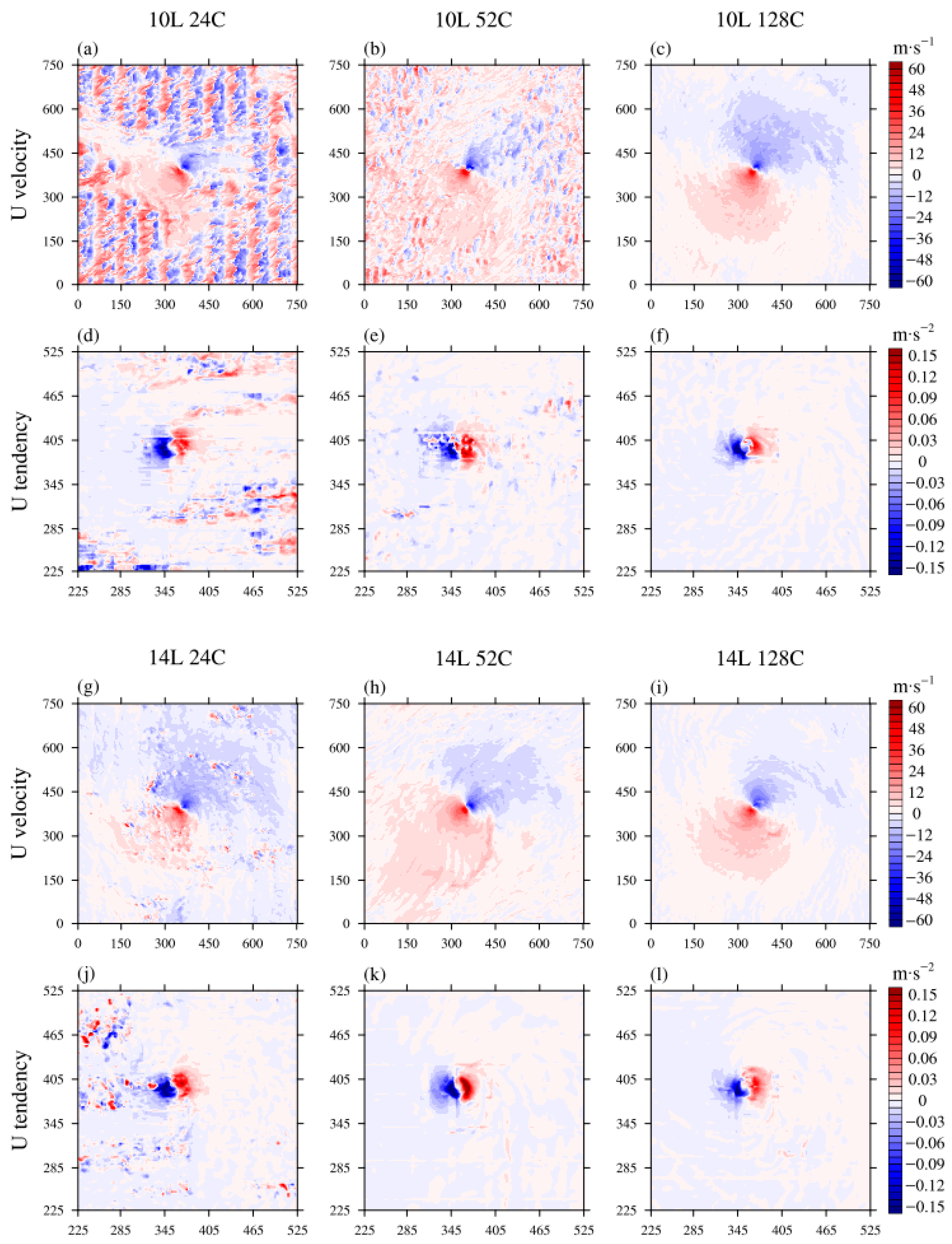
Figure 1 and Figure 2 present the lowest-level $U$-wind field and the corresponding neural-network-predicted $U$-wind tendency after 6 h of WRF integration. Because upper-level results exhibit similar but weaker patterns, only the lowest-level fields are shown. The results differ substantially between the two model families. For DeepBL–CNN, the $U$-wind fields display numerous small-scale positive and negative disturbances of considerable amplitude. The 10L24C model produces the strongest perturbations—extending across the entire D01 domain and reaching amplitudes comparable to the tropical cyclone wind speeds themselves (Figure 1a). The disturbances weaken for 10L52C (Figure 1b) and further diminish for 14L24C (Figure 1g). The corresponding $U$-wind tendencies also display numerous small-scale perturbations (Figure 1d,e,j). The intensity and spatial extent of these disturbances in $U$-wind fields and tendencies decrease as the neural networks’ feature map number and depth increase (Figure 1c,h,i,f,k,l).

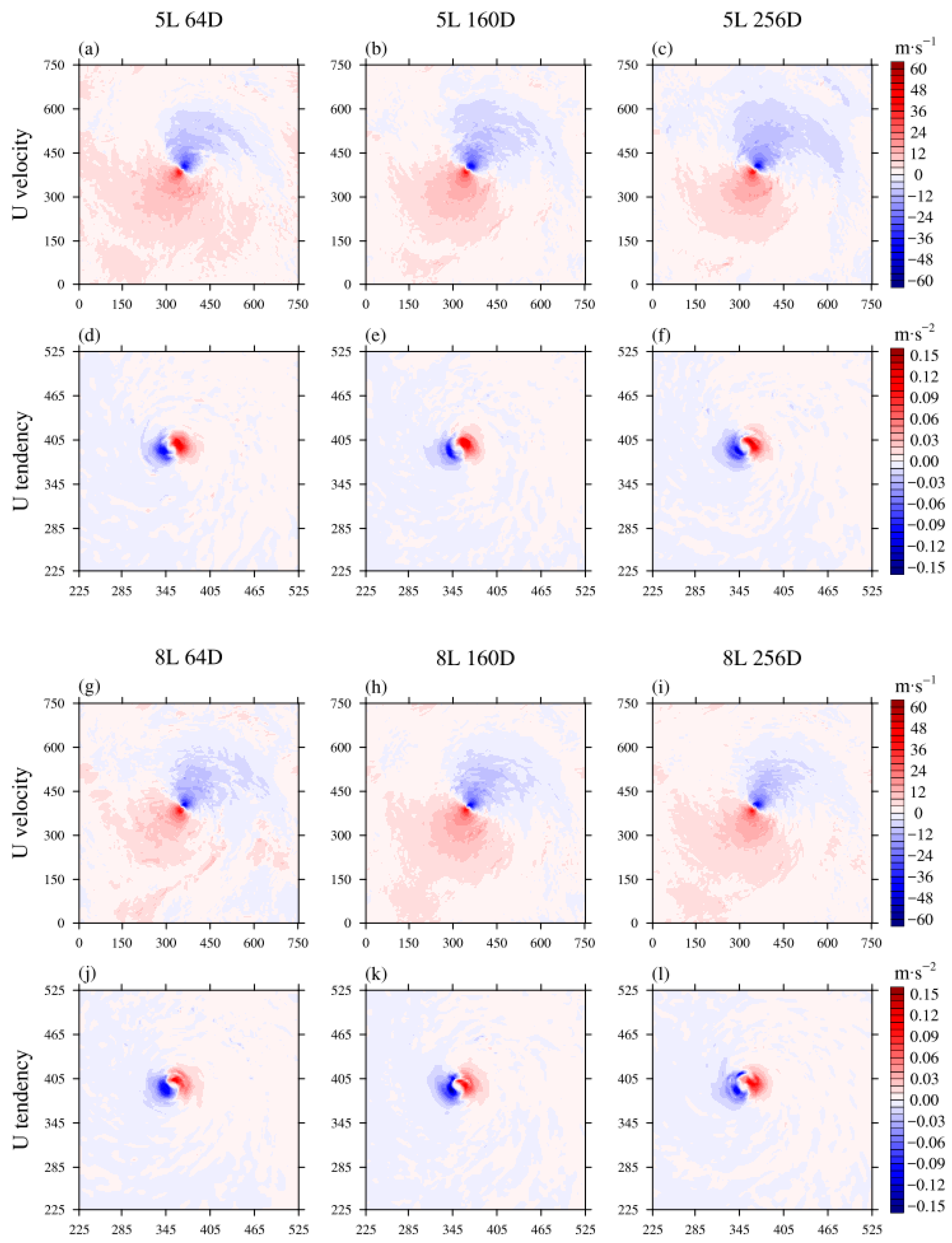
By contrast, DeepBL–FC results exhibit little sensitivity to network configuration. Both the simulated $U$-wind fields and the predicted tendencies remain smooth and physically consistent across all DeepBL–FC variants (Figure 2). Although DeepBL–FC performs worse than DeepBL–CNN on the validation dataset (Table 1 and Table 2), it produces far more stable and realistic behavior in WRF. Simulation results for $V, \Theta$, and $Q$, along with their tendencies, are provided in the Supplementary Materials and closely resemble those of $U$-wind field.

3.3. Influence of Neural Network Structure on Integration Instability

3.3.1. Output Sensibility of DeepBL–CNN on Instable Points

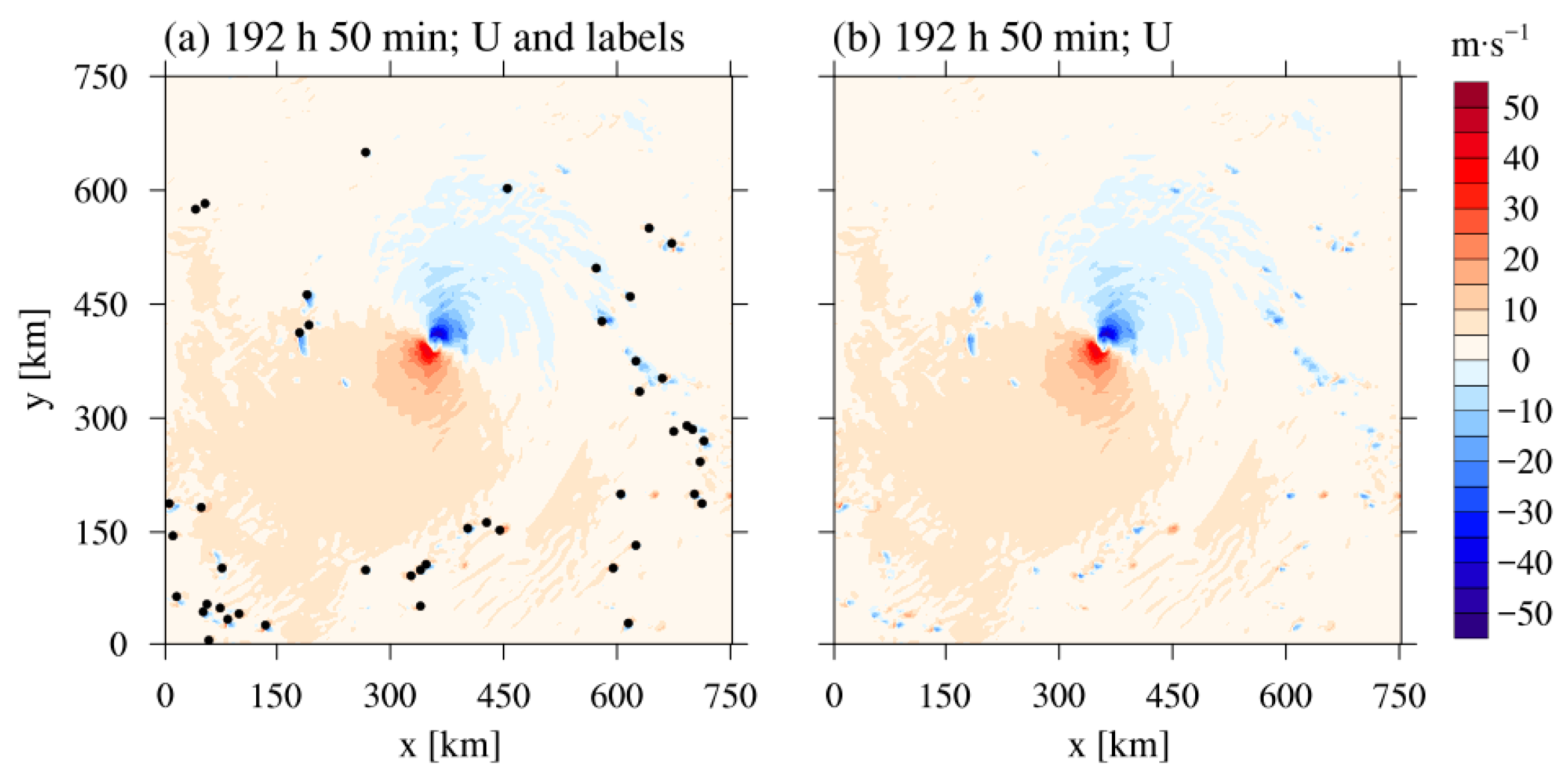
We next investigate the early stage of the instabilities produced by DeepBL–CNN in the WRF simulations. We choose the 10L52C model as an example. Figure 3a illustrates the positions of “instability points.” In the first-layer $U$-wind field at 50 min of integration (Figure 3b), any grid point whose value deviates from the surroundings by more than 40% is labeled as an instability point. As noted in Section 3.2, these instabilities arise primarily within the atmospheric boundary layer; accordingly, we identify instability points within the lowest five model levels at the horizontal locations shown in Figure 3a. Examining how DeepBL–CNN stimulates the early growth of these instabilities during model integration provides insight into the mechanisms that ultimately lead to integral instability.

The instability observed in the wind field in Figure 3b must originate from the behavior of DeepBL–CNN at earlier stages of the integration. We calculate the neural-network-predicted flux difference at the instability points between the WRF simulation time of 30 min and 40 min and contrast the differences with DeepBL–FC. Let ${Flux}_{CNN,40}$ denote the flux predicted by DeepBL–CNN at the instability points at 40 min, and ${Flux}_{CNN,30}$ the corresponding predictions at 30 min. The difference in flux prediction by DeepBL–CNN over this interval is therefore:

$${Diff}_{CNN}=\left|{Flux}_{CNN,40}-{Flux}_{CNN,30}\right|.$$

(8)

We compare ${Diff}_{CNN}$ with those from the DeepBL–FC model of 5L160D. Similarly, the difference in flux predictions by DeepBL–FC between 30 and 40 min is given by:

$${Diff}_{FCNN}=\left|{Flux}_{FCNN,40}-{Flux}_{FCNN,30}\right|.$$

(9)

Subtracting Equation (9) from Equation (8), we obtain:

$${Diff}_{NN}={Diff}_{CNN}-{Diff}_{FCNN}.$$

(10)

The quantity ${Diff}_{NN}$ measures how the flux-prediction change produced by DeepBL–CNN differs from that produced by DeepBL–FC at the instability points. A positive (negative) value of ${Diff}_{NN}$ indicates that under the same input perturbation between 30 and 40 min of integration, DeepBL–CNN produces a larger (smaller) response than DeepBL–FC. Thus, Equation (10) provides a metric for assessing the robustness of the two neural-network architectures to input perturbations.

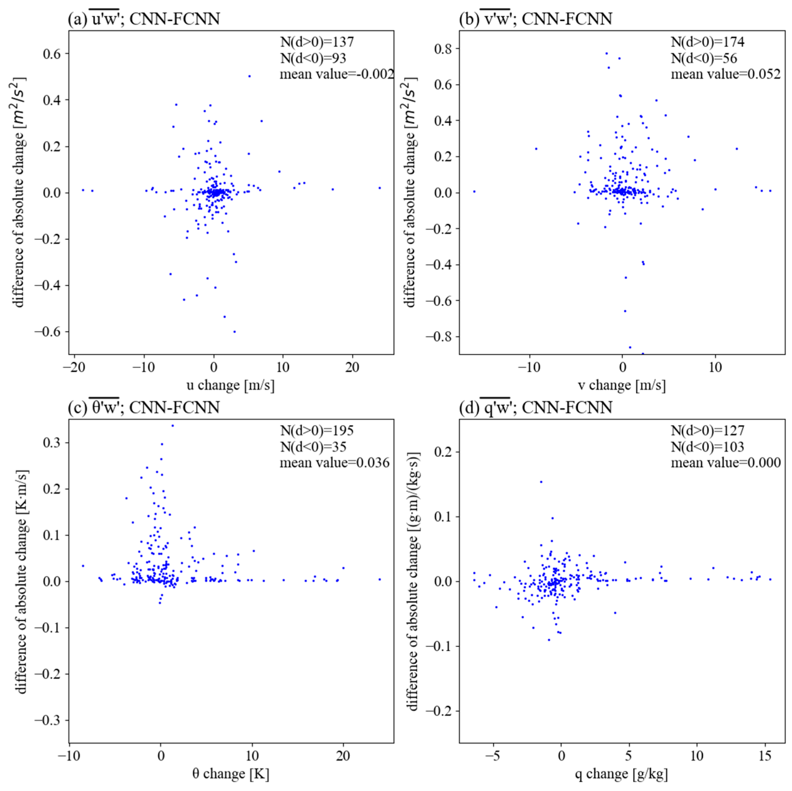
Figure 4 shows the distribution of ${Diff}_{NN}$ for the four flux components at the unstable points, where the horizontal axis represents the changes in the resolved variables between 30 and 40 min. The vertical axis in each subplot corresponds to the tendency induced by the turbulent flux, which directly affects the associated resolved variable on the horizontal axis. Most points cluster near the y-axis, indicating that the instabilities have not yet fully developed by 40 min and that changes in the resolved variables remain small at most instability points. However, for all four flux components, the number of points with ${Diff}_{NN}>0$ exceeds those with ${Diff}_{NN}<0$. For $\overline{v^{\prime }{w}^{\prime }}$ and $\overline{q^{\prime }{w}^{\prime }}$, the number of unstable points with ${Diff}_{NN}>0$ is more than three times that of ${Diff}_{NN}<0$, and the mean value of ${Diff}_{NN}$ is significantly positive. As shown in Figure 4b,c, among the unstable points with relatively large $\left|{Diff}_{NN}\right|$, positive values are far more common than negative ones. These results indicate that under the same perturbations in the input profiles between 30 and 40 min, the resulting perturbations in the DeepBL–CNN outputs are substantially larger. In the following analysis, all DeepBL–CNNs refer to the 10L52C model, and all DeepBL–FCs refer to the 5L160D model.

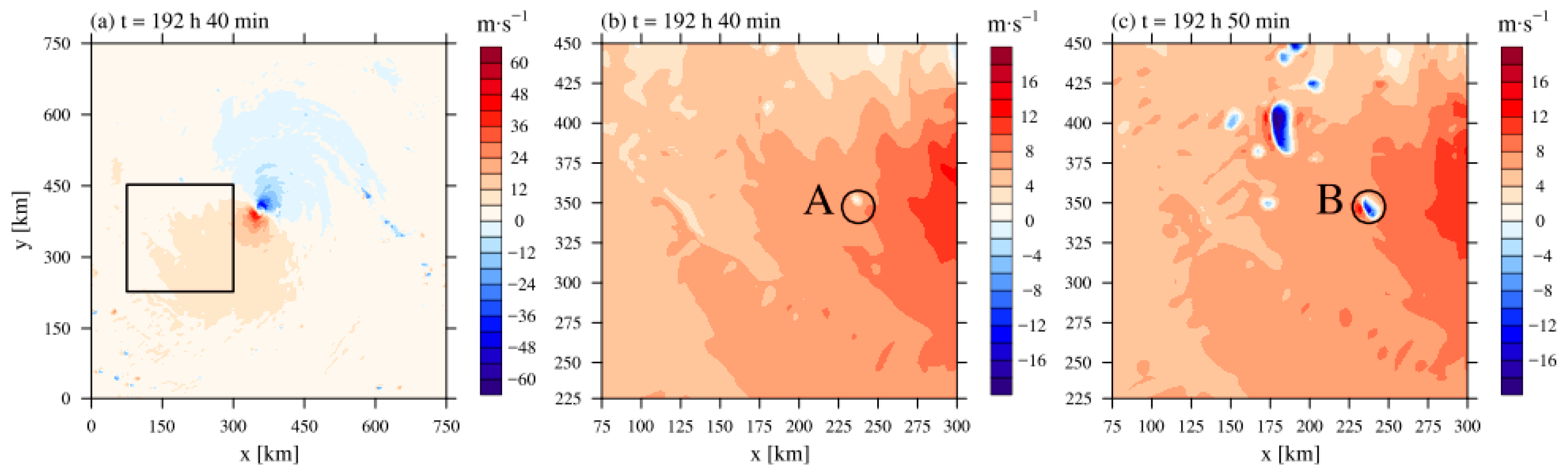
What will happen when DeepBL–CNN is considerably more sensitive to input perturbations than DeepBL–FC? To address this question, we examine a representative location, point A, in the WRF simulation that employs DeepBL–CNN as the boundary-layer scheme. The position of point A is marked in Figure 5b. At 40 min into the WRF integration, point A shows only a slight perturbation, with wind speeds marginally lower than those of the surrounding environment. Yet within the next 10 min, this weak perturbation evolves into an unstable disturbance (point B) characterized by large negative wind speeds (Figure 5c). At the same time, an extended region of similar disturbances appears to the upper left of point B.

We examine how the predicted turbulent flux at point A changes between 30 and 40 min (the same interval in Figure 4) with DeepBL–CNN and DeepBL–FC. We further investigate how these changes contribute to the evolution of point A into the unstable disturbance observed at point B.

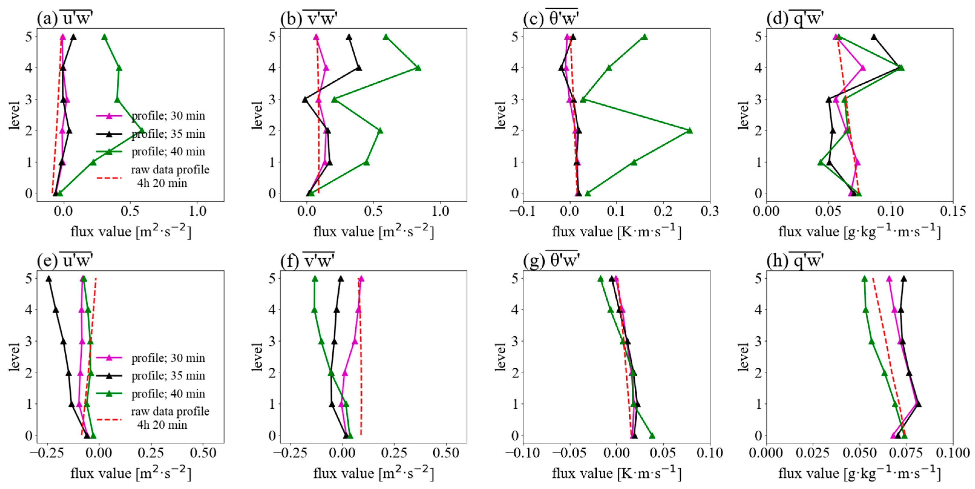
Figure 6 compares the flux profiles produced by DeepBL–CNN and DeepBL–FC when their inputs are the resolved-variable profiles at point A from the WRF simulation (with DeepBL–CNN as the parameterization scheme) at 30, 35, and 40 min. For DeepBL–CNN, when the input is the 30 min profile, the predicted turbulent-flux profiles closely match those diagnosed from the LES (dashed lines in Figure 6). With the 35 min input, however, the $\overline{v^{\prime }{w}^{\prime }}$ profile begins to deviate substantially from the LES profiles at the 4th and 5th levels, while differences remain small in the lower levels (Figure 6b). A similar pattern appears for $\overline{q^{\prime }{w}^{\prime }}$: fluxes at the 4th and 5th levels increase markedly, whereas those at the 1st–3rd levels decrease slightly (Figure 6d). The $\overline{u^{\prime }{w}^{\prime }}$ and $\overline{{\theta }^{\prime }{w}^{\prime }}$ profiles remain basically unchanged (Figure 6a,c).

Only five minutes later, DeepBL–CNN’s predictions of $\overline{u^{\prime }{w}^{\prime }}$, $\overline{v^{\prime }{w}^{\prime }}$, and $\overline{{\theta }^{\prime }{w}^{\prime }}$ change dramatically (Figure 6a–c), with magnitudes differing by factors of tens relative to the LES profiles. Although the absolute change in $\overline{q^{\prime }{w}^{\prime }}$ is smaller, its vertical gradient increases sharply (Figure 6d). Because the surface fluxes (level 0) change only slightly, the tendencies imposed by DeepBL–CNN on $U$, $V$, $\Theta$, and $Q$ at the first model level increase substantially.

At 40 min, the tendencies predicted by DeepBL–CNN for $U$, $V$, $\Theta$, and $Q$ are −0.01 m s⁻¹, −0.018 m s⁻¹, −0.005 K s⁻¹, and 0.00125 g kg⁻¹ s⁻¹, respectively. Over the subsequent 10 min, these tendencies produce changes of −6 m s⁻¹, −10.8 m s⁻¹, −3 K, and 0.75 g kg⁻¹. In the WRF simulation, the corresponding changes at point A between 40 and 50 min are −4.16 m s⁻¹, −3.60 m s⁻¹, 0.06 K, and 1.05 g kg⁻¹. Except for $\Theta$, the predicted and simulated changes agree closely.

In contrast, DeepBL–FC behaves markedly differently from DeepBL–CNN. For DeepBL–FC, the flux profiles predicted using the 30 and 35 min inputs remain close to the LES profiles, and even the 40 min input does not produce the abrupt changes observed in DeepBL–CNN.

Taken together, Figure 5 and Figure 6 show that variations in the WRF input profiles between 30 and 40 min induce pronounced fluctuations in the flux profiles predicted by DeepBL–CNN at specific unstable points. These fluctuations serve as the immediate trigger for the onset of instability. The same perturbations, however, produce no comparable response in DeepBL–FC, accounting for its much more stable behavior during WRF integration.

3.3.2. Feature Map Sensitivity to the Input Disturbance

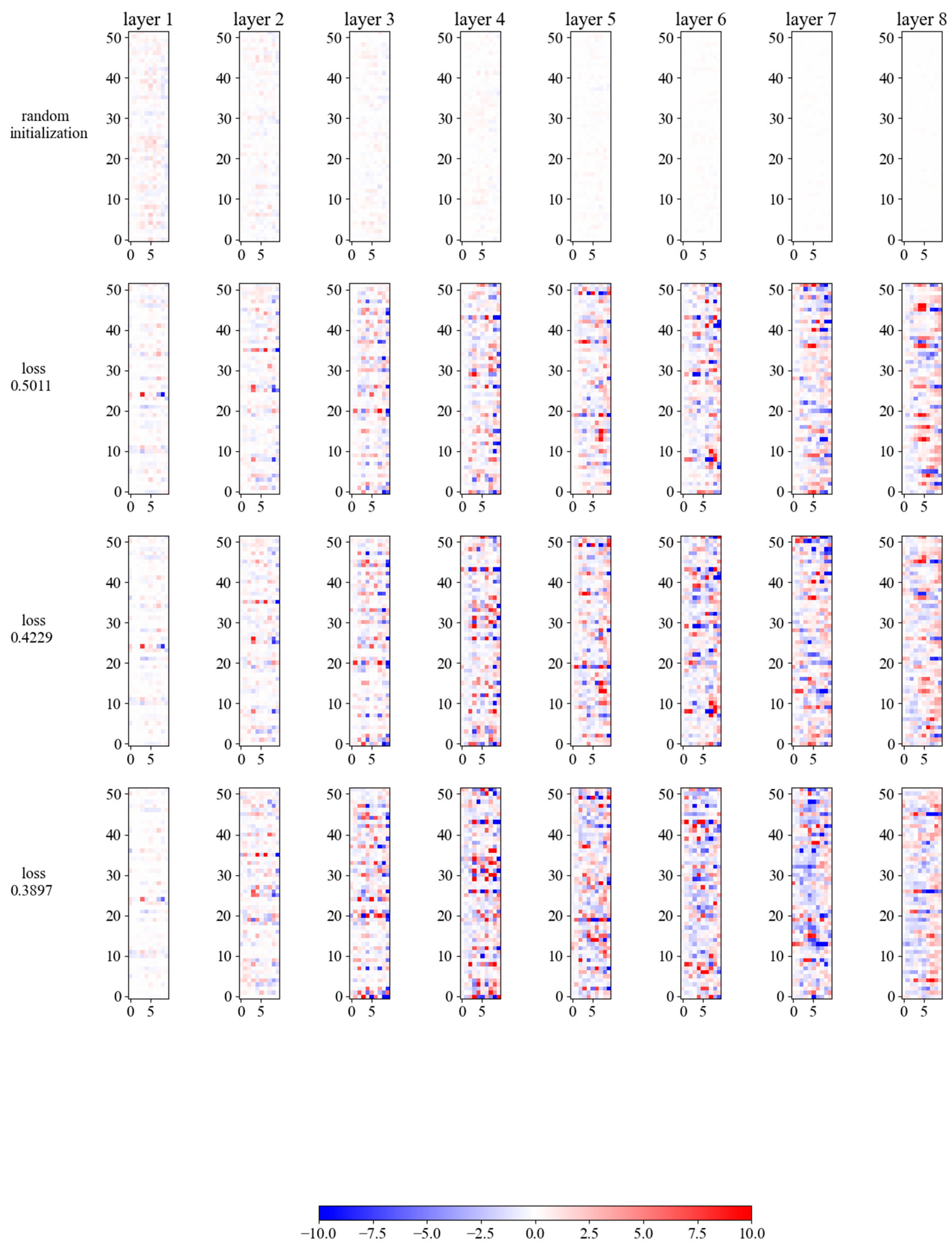
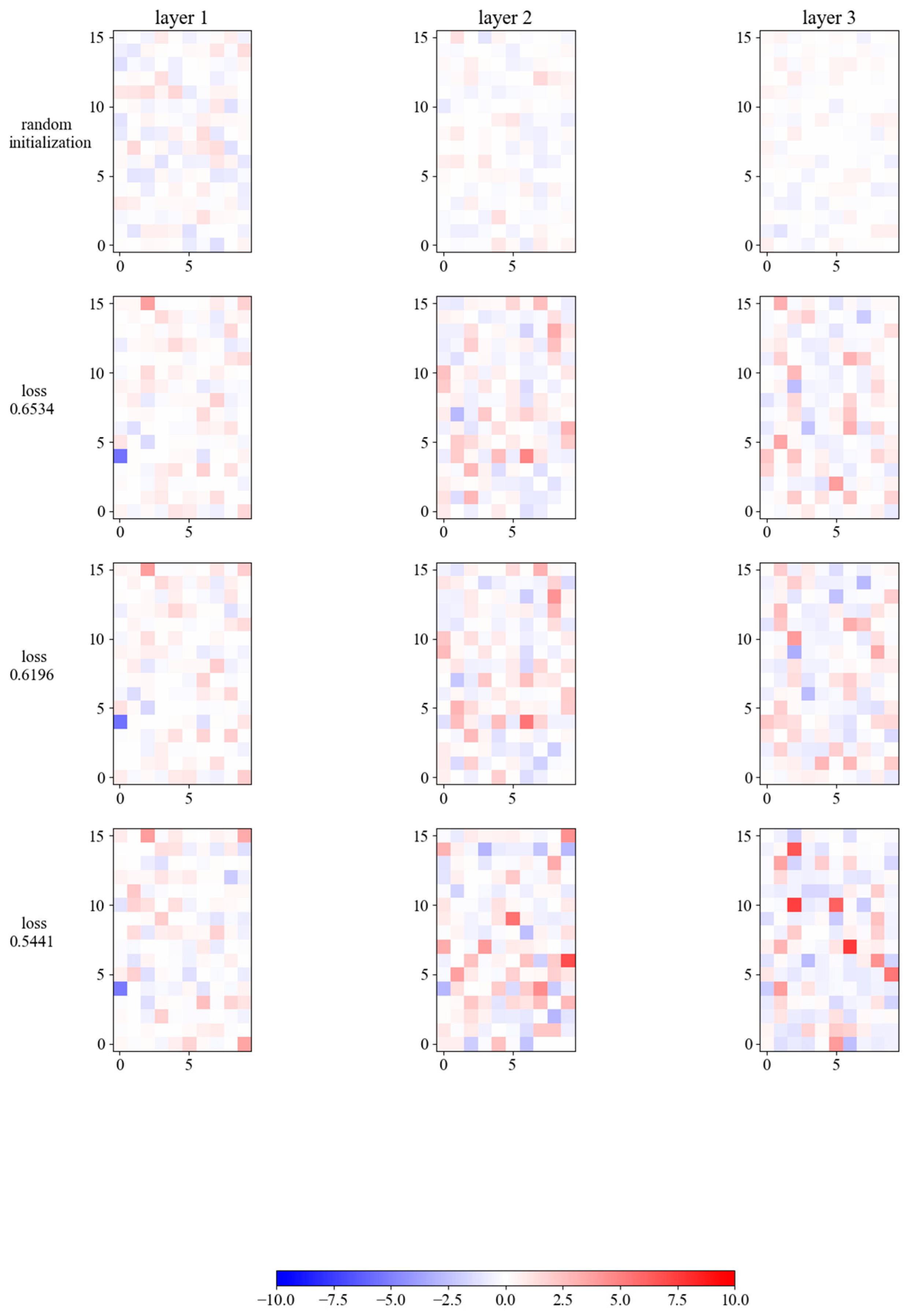
Why does DeepBL–CNN exhibit a much stronger output response than DeepBL–FC under the same input perturbations? Figure 7 and Figure 8 compare the responses of their intermediate layers. We select an arbitrary point from Figure 3a and compute, for each model, the difference between the intermediate-layer outputs obtained using the 40 min input profile and those obtained using the 30 min profile; these differences are shown in Figure 7 and Figure 8.

Figure 7 shows that throughout training, certain channels in DeepBL–CNN’s intermediate layers display extremely large responses. Pronounced discrepancies occur both between adjacent channels and between successive layers, producing highly heterogeneous response patterns across the network. As the perturbation propagates toward the output layer, the response magnitude grows progressively, revealing a strong layer-by-layer amplification. In contrast, Figure 8 indicates that DeepBL–FC behaves very differently. Its intermediate-layer responses are substantially smaller and far more uniform, and the pronounced amplification observed in DeepBL–CNN is largely absent.

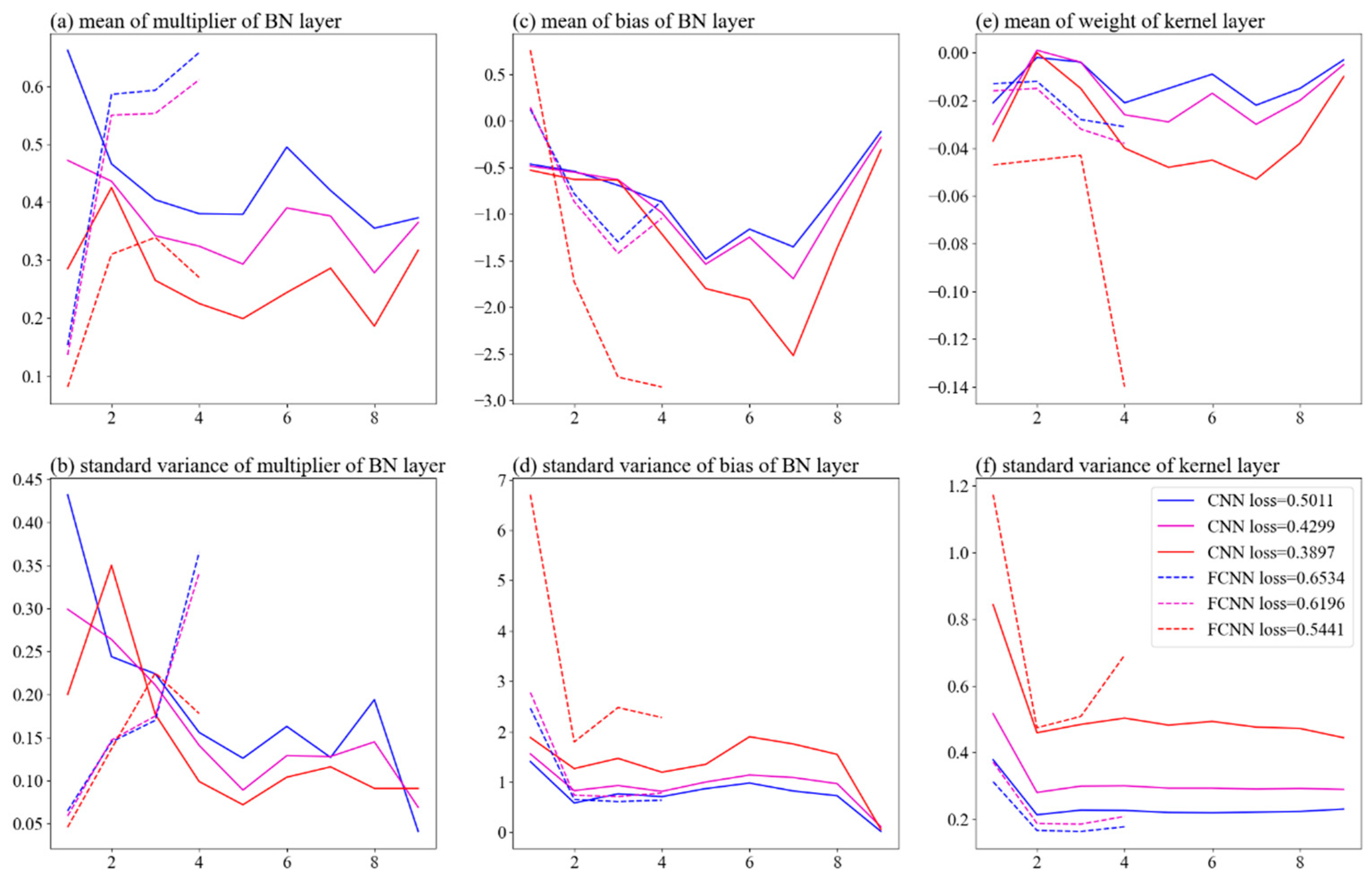
Is the difference in response attributable to substantial differences in the network weights of the two models? To investigate this, we examined the means and variances of the batch-normalization (BN) layers and kernel layers of DeepBL–CNN and DeepBL–FC at several training stages. As shown in Figure 9, the overall magnitudes of the network weights do not differ appreciably between the two networks. In fact, the BN bias means (Figure 9c), BN bias standard deviations (Figure 9d), and kernel-layer means (Figure 9e) of the lowest-loss DeepBL–FC model are larger than those of the other networks.

Thus, the striking differences in intermediate-layer responses seen in Figure 7 and Figure 8 cannot be explained by differences in BN or kernel parameter magnitudes. Moreover, Figure 7 shows that the large activations in DeepBL–CNN emerge early in training, indicating that they are not a consequence of overfitting but rather an intrinsic feature of the DeepBL–CNN architecture in this study.

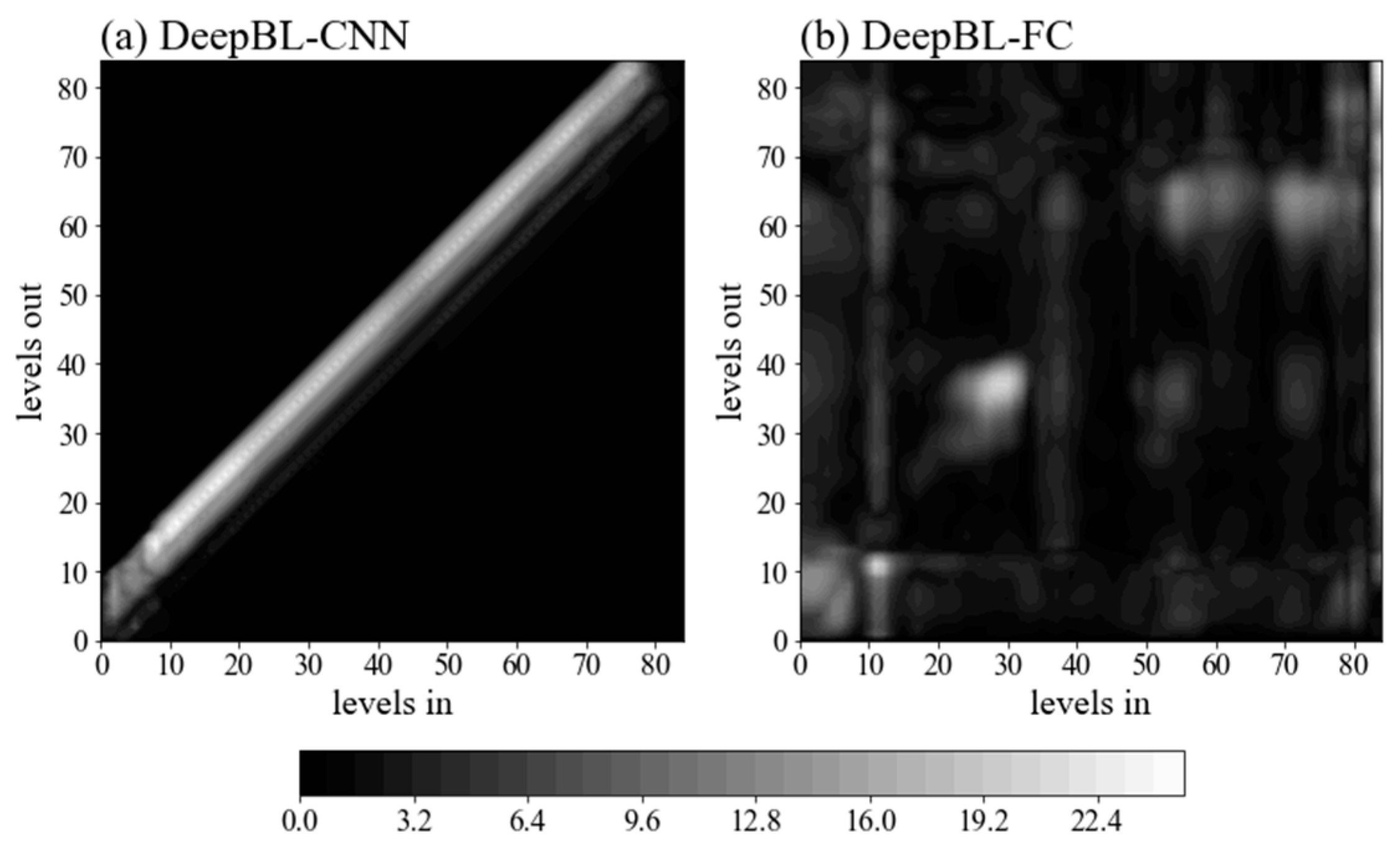
Why does the convolutional architecture of DeepBL–CNN produce the behavior observed in Figure 7? Figure 10 compares the input sensitivities of DeepBL–CNN and DeepBL–FC. We perturb the input at a selected layer and evaluate the resulting output responses across all layers. DeepBL–CNN exhibits narrow, stripe-like sensitivity patterns aligned along the diagonal of the two-dimensional response matrix, with negligible responses outside this diagonal band. By contrast, DeepBL–FC shows more diffuse and uniformly distributed sensitivities across the entire matrix. In addition, the magnitude of the output response is substantially larger for DeepBL–CNN than for DeepBL–FC. In summary, DeepBL–CNN exhibits highly concentrated and amplified sensitivities, whereas DeepBL–FC displays smaller, more spatially uniform responses.

This sensitivity pattern arises directly from the network architectures. In DeepBL–CNN, the convolutional structure restricts how perturbations propagate: a perturbation introduced at a given height can only influence neighboring levels. For instance, a perturbation applied at level 10 affects only levels 9–11 in the next hidden layer due to the kernel size of 3. In the following layer, the influence spreads only to levels 8–12, and so on, with levels closer to level 10 receiving a larger share of the perturbation. This localized and gradually expanding propagation produces the narrow, diagonal band of sensitivity observed in DeepBL–CNN.

DeepBL–FC behaves differently because every neuron in a hidden layer is fully connected to all neurons in adjacent layers. Consequently, a perturbation introduced at any level can propagate throughout the entire network. This produces a sensitivity pattern that is more uniform and spatially diffuse, in contrast to the highly localized response confined to the vicinity of the perturbed level in DeepBL–CNN.

The output sensitivity of CNN might also be highly relevant with the adversarial perturbations, which can cause a large output response even if the input perturbations are of small amplitude. Goodfellow et al. [46] argued that the CNN can be viewed as a linear model in high-dimensional spaces when the input perturbations are small. When perturbations are highly aligned with the weight vectors of CNN, even if the perturbations are small, a CNN can still aggregate thousands of these small changes across its layers. These small perturbations add up to a massive shift in the final output of CNN. For a small model like DeepBL–CNN, the possibility that input perturbations are highly aligned with weight vectors of DeepBL–CNN might not be low, which will cause the output abrupt change.

In summary, the one-dimensional convolutional architecture of DeepBL–CNN allows perturbations in certain input profiles to accumulate progressively across layers without being effectively distributed to neighboring vertical levels. This results in a gradual amplification of perturbation amplitudes, making the convolutional network inherently more sensitive to input disturbances. DeepBL–CNN might also produce abrupt output change due to the adversarial perturbations of neural network. In contrast, DeepBL–FC does not exhibit this behavior: its fully connected structure enables perturbations at a single level to spread across all neurons in the subsequent layer, dispersing the disturbance signal and preventing layer-by-layer amplification.

3.4. Stable Integration of DeepBL–CNN in WRF Model

3.4.1. How to Stabilize Integration of DeepBL–CNN

This section investigates methods for stabilizing the integration of DeepBL–CNN within the WRF model. The first approach is data augmentation by adding Gaussian noise to the training data. To mitigate the large output fluctuations DeepBL–CNN exhibits in response to specific input perturbations, small random perturbations can be added to both the inputs and outputs during training. With sufficient training, the network learns to produce stable outputs for a wide range of perturbed input profiles, effectively reducing its sensitivity to input disturbances. Adding noise to training data is important for a robust model. Training data are always distributed on a manifold in high-dimensional space, and the model’s behavior is not predictable when input data are not on the manifold, which is not rare. Adding noise will change the manifold into a space with volume, which will cover the input data not on the manifold.

The second approach is spectral-norm regularization [47]. As discussed in Section 3.3.2, the instability of DeepBL–CNN within the WRF model stems from the progressive, layer-by-layer amplification of certain input perturbations, which ultimately produces large output fluctuations. Constraining the sensitivity of intermediate-layer outputs to input perturbations can therefore help mitigate this instability. This constraint can be expressed equivalently as a bound on the spectral norms of the convolution kernels, with the derivation provided in Supplementary Materials.

The third approach is L2 regularization, which constrains the Frobenius norms of the DeepBL–CNN convolution kernels and achieves effects similar to spectral-norm regularization. However, it imposes a stricter constraint than the spectral-norm bound. The corresponding derivation is provided in the Supplementary Materials.

3.4.2. Comparisons Between the Three Methods

This study evaluates how different Gaussian-noise intensities and regularization strengths affect ${Diff}_{NN}$ at unstable points for DeepBL–CNN. For Gaussian noise augmentation, noise is added to both inputs and outputs, drawn from a zero-mean Gaussian distribution with variance equal to $\alpha$ times the standard deviation of the corresponding variable. For spectral-norm regularization, constraints are applied to all convolution kernels in each layer of DeepBL–CNN, using five power-iteration steps; the regularization coefficient is denoted by $\beta$. L2 regularization is likewise applied to all convolution kernels in each layer of DeepBL–CNN, with the coefficient in front of the regularization term denoted by $\gamma$.

Table 3. Weighing coefficients of the three methods.

Weighing Coefficients	Coefficient Value
$\alpha$	1 × 10−4	2 × 10−4	5 × 10−4	1 × 10−3	2 × 10−3	5 × 10−3	1 × 10−2
$\beta$	2 × 10−5	5 × 10−5	1 × 10−4	1 × 10−3	1 × 10−2
$\gamma$	1 × 10−6	1 × 10−5	1 × 10−4	1 × 10−3	1 × 10−2

lists the values of $\alpha$, $\beta$, and $\gamma$ used during training.

For each choice of weighting coefficients, the model is trained for 25 epochs, and the DeepBL–CNN at the end of each epoch is saved. Following the analysis in Section 3.3.1, if the improved DeepBL–CNN predicts the flux at an unstable point at 40 min as ${Flux}_{CNN\text{-}opt,40}$ and at 30 min as ${Flux}_{CNN\text{-}opt,30}$, then the corresponding 30–40 min flux difference for the improved model is defined as:

$${Diff}_{CNN\text{-}opt}=\left|{Flux}_{CNN\text{-}opt,40}-{Flux}_{CNN\text{-}opt,30}\right|.$$

(11)

Similar to Section 3.3.1, for each neural network model, we compute the mean value of ${Diff}_{NN\text{-}opt}$ for all four flux types across all unstable points. By replacing ${Diff}_{FCNN}$ in Equation (10) of Section 3.3.1 with ${Diff}_{CNN\text{-}opt}$, we obtain the formulation for calculating ${Diff}_{NN\text{-}opt}$:

$${Diff}_{NN\text{-}opt}={Diff}_{CNN}-{Diff}_{CNN\text{-}opt}.$$

(12)

Before averaging, the values of ${Diff}_{NN\text{-}opt}$ for the four flux components are normalized to the range of 0–1. A larger mean ${Diff}_{NN\text{-}opt}$ indicates that the corresponding neural network is less sensitive to input perturbations at unstable points than the original DeepBL–CNN. We rank all networks in descending order of their mean ${Diff}_{NN\text{-}opt}$ and select the top 60 models. Among these, 22 are obtained using Gaussian-noise augmentation, 18 using spectral-norm regularization, and 20 using L2 regularization. Notably, nine of the top ten models adopt L2 regularization. These results show that all three approaches reduce the sensitivity of DeepBL–CNN to input perturbations, with L2 regularization—which imposes a stronger constraint than spectral normalization—yielding the most substantial improvement.

We further select DeepBL–CNN models that exhibit both relatively large ${Diff}_{NN\text{-}opt}$ values and strong validation performance, and compare the numbers of unstable points satisfying ${Diff}_{NN\text{-}opt}>0$ and ${Diff}_{NN\text{-}opt}<0$, as well as the magnitudes of ${Diff}_{NN\text{-}opt}$. The results are summarized in

Table 4. ${Diff}_{NN\text{-}opt}$ on instability points by DeepBL–CNN after optimized by the three methods.

Neural Network		$\overline{{\mathit{u}}^{\mathbf{\prime }}{\mathit{w}}^{\mathbf{\prime }}}$	$\overline{{\mathit{v}}^{\mathbf{\prime }}{\mathit{w}}^{\mathbf{\prime }}}$	$\overline{{\mathit{\theta }}^{\mathbf{\prime }}{\mathit{w}}^{\mathbf{\prime }}}$	$\overline{{\mathit{q}}^{\mathbf{\prime }}{\mathit{w}}^{\mathbf{\prime }}}$
$loss=0.658$ $\alpha =5\times {10}^{-4}$	${Diff}_{NN\text{-}opt}>0$	176	176	147	176
	${Diff}_{NN\text{-}opt}<0$	54	54	83	54
	${Diff}_{NN\text{-}opt}$ mean	4.75 × 10−2	8.61 × 10−2	2.23 × 10−2	1.33 × 10−2
$loss=0.5842$ $\alpha =1\times {10}^{-4}$	${Diff}_{NN\text{-}opt}>0$	155	177	158	154
	${Diff}_{NN\text{-}opt}<0$	75	53	72	76
	${Diff}_{NN\text{-}opt}$ mean	3.16 × 10−2	8.77 × 10−2	2.17 × 10−2	9.34 × 10−3
$loss=0.6469$ $\alpha =5\times {10}^{-3}$	${Diff}_{NN\text{-}opt}>0$	174	167	175	159
	${Diff}_{NN\text{-}opt}<0$	56	63	55	71
	${Diff}_{NN\text{-}opt}$ mean	4.02 × 10−2	6.85 × 10−2	3.14 × 10−2	8.72 × 10−3
$loss=0.549$ $\beta =2\times {10}^{-5}$	${Diff}_{NN\text{-}opt}>0$	153	180	176	135
	${Diff}_{NN\text{-}opt}<0$	77	50	54	95
	${Diff}_{NN\text{-}opt}$ mean	4.68 × 10−2	8.38 × 10−2	3.11 × 10−2	6.12 × 10−3
$loss=0.6207$ $\beta =1\times {10}^{-3}$	${Diff}_{NN\text{-}opt}>0$	151	180	178	151
	${Diff}_{NN\text{-}opt}<0$	79	50	52	79
	${Diff}_{NN\text{-}opt}$ mean	2.91 × 10−2	6.73 × 10−2	3.03 × 10−2	8.41 × 10−2
$loss=0.6069$ $\beta =1\times {10}^{-4}$	${Diff}_{NN\text{-}opt}>0$	147	175	151	144
	${Diff}_{NN\text{-}opt}<0$	83	55	79	86
	${Diff}_{NN\text{-}opt}$ mean	3.09 × 10−2	7.57 × 10−2	2.40 × 10−2	7.55 × 10−2
$loss=0.5434$ $\gamma =1\times {10}^{-6}$	${Diff}_{NN\text{-}opt}>0$	165	191	169	166
	${Diff}_{NN\text{-}opt}<0$	65	39	61	64
	${Diff}_{NN\text{-}opt}$ mean	5.41 × 10−2	9.35 × 10−2	2.84 × 10−2	1.10 × 10−2
$loss=0.5551$ $\gamma =1\times {10}^{-6}$	${Diff}_{NN\text{-}opt}>0$	174	178	169	168
	${Diff}_{NN\text{-}opt}<0$	56	52	61	62
	${Diff}_{NN\text{-}opt}$ mean	4.75 × 10−2	7.45 × 10−2	2.63 × 10−2	1.00 × 10−2
$loss=0.5071$ $\gamma =1\times {10}^{-6}$	${Diff}_{NN\text{-}opt}>0$	142	178	134	162
	${Diff}_{NN\text{-}opt}<0$	88	52	96	68
	${Diff}_{NN\text{-}opt}$ mean	3.20 × 10−2	8.75 × 10−2	9.83 × 10−3	1.19 × 10−2

. Table 4 shows that for all three methods, the number of unstable points with ${Diff}_{NN\text{-}opt}>0$ is 1.5–3 times larger than those with ${Diff}_{NN\text{-}opt}<0$, and the mean ${Diff}_{NN\text{-}opt}$ is significantly positive. Relative to the DeepBL–FC results in Section 3.3.1, the improved DeepBL–CNN models show markedly reduced sensitivity to input perturbations at unstable points.

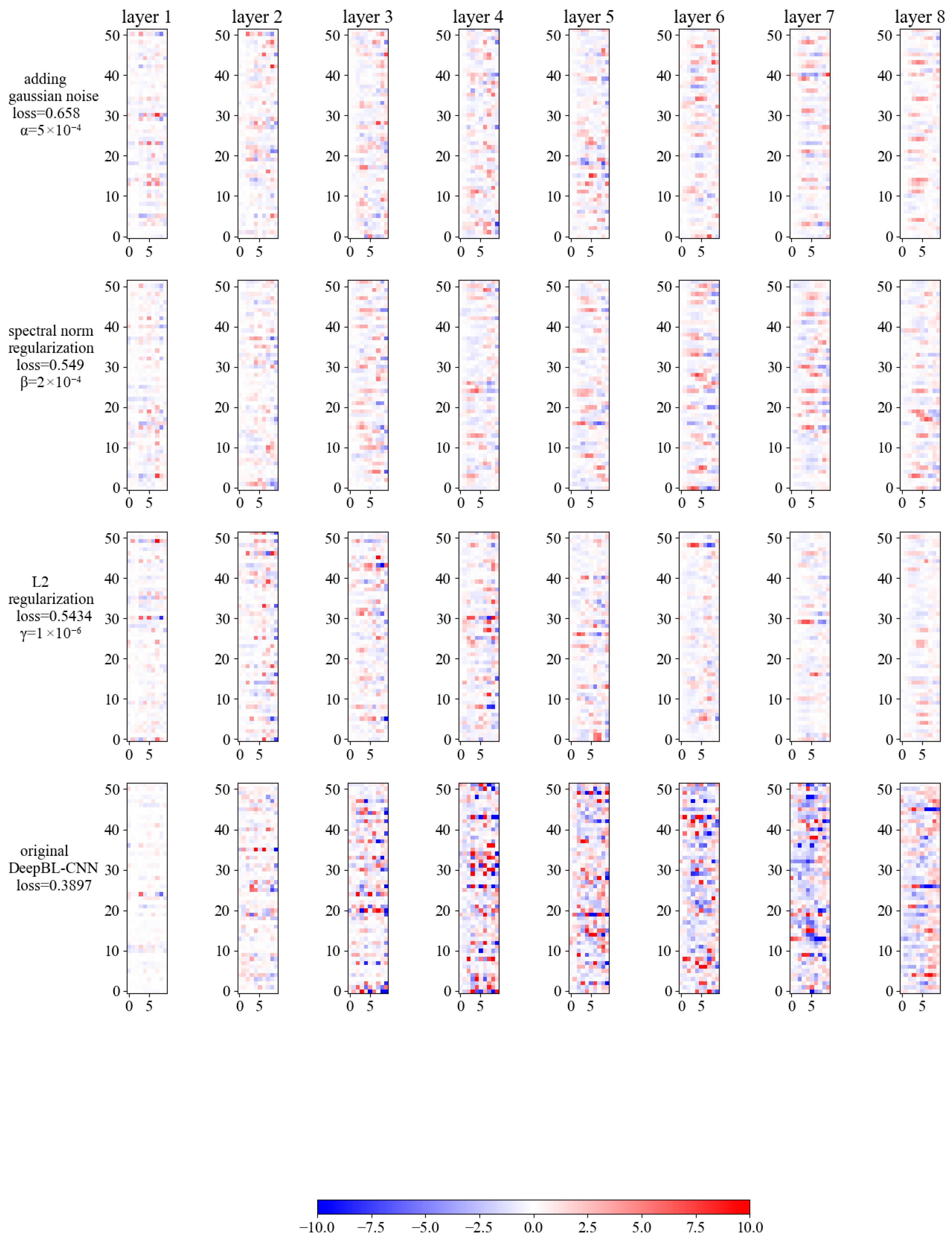
We next examine the same point used in Figure 7 and Figure 8 (from Figure 3a). Following the approach in those figures, Figure 11 compares the intermediate-layer responses of the improved DeepBL–CNN with those of the original model. All three methods introduced in Section 3.4.1 substantially enhance network stability. Compared with the original DeepBL–CNN, the improved models exhibit greatly reduced intermediate-layer response magnitudes, far more uniform amplitudes across layers, and no evidence of layer-by-layer amplification. Instead, the responses generally decline over the final three layers. Consequently, the sensitivity of intermediate-layer activations to input perturbations is significantly reduced. These findings are fully consistent with the results in Table 4.

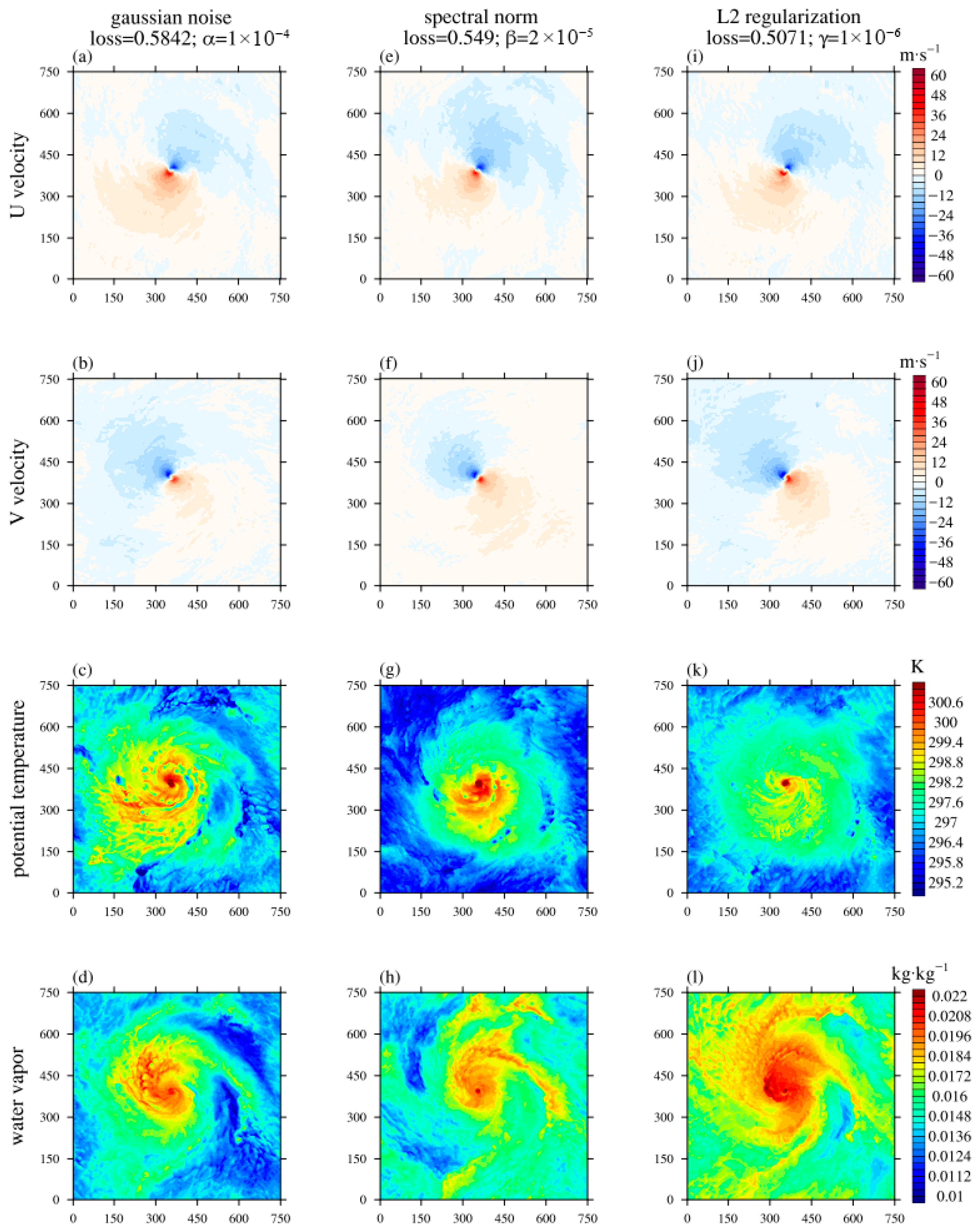
How do the improved DeepBL–CNN models perform in WRF simulations? Using the same initial vortex as in Section 3.2, we replace the boundary-layer scheme with each improved DeepBL–CNN and conduct tropical cyclone simulations. Figure 12 shows the results after 6 h. All three improved DeepBL–CNNs produce well-organized tropical cyclones: the $U$- and $V$-wind fields exhibit clear antisymmetric structures, while the $\Theta$ and $Q$ fields feature a distinct eye, eyewall, and spiral rainbands. The potential temperature field also reveals a sequence of low temperature anomalies, indicative of cold pools generated by convective cells. These results demonstrate that the improved DeepBL–CNN not only integrates stably within the WRF model but also produces physically realistic tropical cyclone simulations.

4. Conclusions

This study investigates the integration stability of the one-dimensional convolutional DeepBL–CNN and the fully connected DeepBL–FC within the WRF model. We systematically examine the factors underlying their differing simulation performance and develop methods to stabilize neural-network-based parameterizations in WRF.

We find that, when initialized with the same tropical cyclone, DeepBL–FC networks with different architectural configurations integrate stably within WRF, whereas all tested DeepBL–CNN configurations develop numerical instabilities. These instabilities appear as widespread, small-scale, large-amplitude oscillations in the model fields. By tracking their evolution, we identify “unstable points” in the velocity fields at 50 min of integration and examine how the neural-network parameterizations respond to changes in the input profiles between 30 and 40 min on those points.

Our analysis shows that at these unstable points, DeepBL–CNN produces far larger output perturbations than DeepBL–FC when subjected to identical input disturbances. This heightened sensitivity generates unrealistic boundary-layer tendencies around 40 min into the integration, which subsequently trigger model blow-up roughly 10 min later. An examination of the intermediate-layer responses further reveals that DeepBL–FC maintains relatively uniform, small-magnitude activations, whereas DeepBL–CNN produces much larger and highly heterogeneous responses across layers and channels. As perturbations propagate forward, this non-uniform amplification intensifies, ultimately giving rise to the pronounced output sensitivity of the CNN.

These contrasting response characteristics stem directly from the architectures of DeepBL–CNN and DeepBL–FC. Because of its limited receptive fields, the convolutional design of DeepBL–CNN restricts the rapid communication of perturbations across neighboring vertical levels, allowing perturbations in specific input profiles to accumulate and grow. This accumulation drives the DeepBL–CNN’s heightened sensitivity to input perturbations. The output sensitivity might also be relevant to the adversarial attack of the neural network [46]. By contrast, the fully connected architecture of DeepBL–FC disperses perturbations across all levels instantaneously, effectively suppressing such buildup.

Finally, we assess three techniques for improving the stability of DeepBL–CNN within WRF—adding Gaussian noise to the training data, applying spectral-norm regularization, and using L2 regularization. All three approaches substantially reduce the model’s sensitivity to input perturbations. At unstable points, the enhanced DeepBL–CNNs exhibit lower sensitivity to input-profile preturbations than DeepBL–FC. An analysis of intermediate-layer responses further shows that these methods successfully suppress the amplitude, variability, and layer-by-layer accumulation of perturbation responses within DeepBL–CNN. WRF simulations confirm that the improved DeepBL–CNNs remain stable for more than 6 h on tropical cyclone simulations.

Recently, incorporating physical laws into neural networks for reliable applications of machine learning in numerical simulations, or physics-informed neural networks [48,49,50,51,52], has received wide attention. Future work should be focused on how to combine more physical laws with neural-network-based parameterization schemes for generalizability towards wider applications.

References

1. Bertoli, G.; Mohebi, S.; Ozdemir, F.; Jucker, J.; Rüdisühli, S.; Perez-Cruz, F.; Salzmann, M.; Schemm, S. Revisiting machine learning approaches for short-and longwave radiation inference in weather and climate models. J. Adv. Model. Earth Syst. 2025, 17, e2025MS004956. [Google Scholar] [CrossRef] [Scilit]
2. Meyer, D.; Hogan, R.J.; Dueben, P.D.; Mason, S.L. Machine learning emulation of 3D cloud radiative effects. J. Adv. Model. Earth Syst. 2022, 14, e2021MS002550. [Google Scholar] [CrossRef] [Scilit]
3. Roh, S.; Song, H.J. Evaluation of neural network emulations for radiation parameterization in cloud resolving model. Geophys. Res. Lett. 2020, 47, e2020GL089444. [Google Scholar] [CrossRef] [Scilit]
4. Song, H.J.; Roh, S. Improved weather forecasting using neural network emulation for radiation parameterization. J. Adv. Model. Earth Syst. 2021, 13, e2021MS002609. [Google Scholar] [CrossRef] [Scilit]
5. Ukkonen, P. Exploring pathways to more accurate machine learning emulation of atmospheric radiative transfer. J. Adv. Model. Earth Syst. 2022, 14, e2021MS002875. [Google Scholar] [CrossRef] [Scilit]
6. Yao, Y.; Zhong, X.; Zheng, Y.; Wang, Z. A physics-incorporated deep learning framework for parameterization of atmospheric radiative transfer. J. Adv. Model. Earth Syst. 2023, 15, e2022MS003445. [Google Scholar] [CrossRef] [Scilit]
7. Harder, P.; Watson-Parris, D.; Stier, P.; Strassel, D.; Gauger, N.R.; Keuper, J. Physics-informed learning of aerosol microphysics. Environ. Data Sci. 2022, 1, e20. [Google Scholar] [CrossRef] [Scilit]
8. Gettelman, A.; Gagne, D.J.; Chen, C.C.; Christensen, M.W.; Lebo, Z.J.; Morrison, H.; Gantos, G. Machine learning the warm rain process. J. Adv. Model. Earth Syst. 2021, 13, e2020MS002268. [Google Scholar] [CrossRef] [Scilit]
9. Seifert, A.; Siewert, C. An ML-based P3-like multimodal two-moment ice microphysics in the ICON model. J. Adv. Model. Earth Syst. 2024, 16, e2023MS004206. [Google Scholar] [CrossRef] [Scilit]
10. Sharma, S.; Greenberg, D.S. SuperdropNet: A stable and accurate machine learning proxy for droplet-based cloud microphysics. J. Adv. Model. Earth Syst. 2025, 17, e2024MS004279. [Google Scholar] [CrossRef] [Scilit]
11. Cheng, Y.; Giometto, M.G.; Kauffmann, P.; Lin, L.; Cao, C.; Zupnick, C.; Li, H.; Li, Q.; Huang, Y.; Abernathey, R.; et al. Deep learning for subgrid-scale turbulence modeling in large-eddy simulations of the convective atmospheric boundary layer. J. Adv. Model. Earth Syst. 2022, 14, e2021MS002847. [Google Scholar] [CrossRef] [Scilit]
12. Pal, A. Deep learning emulation of subgrid-scale processes in turbulent shear flows. Geophys. Res. Lett. 2020, 47, e2020GL087005. [Google Scholar] [CrossRef] [Scilit]
13. Subel, A.; Chattopadhyay, A.; Guan, Y.; Hassanzadeh, P. Data-driven subgrid-scale modeling of forced Burgers turbulence using deep learning with generalization to higher Reynolds numbers via transfer learning. Phys. Fluids 2021, 33, 031702. [Google Scholar] [CrossRef] [Scilit]
14. Vinuesa, R.; Brunton, S.L. Enhancing computational fluid dynamics with machine learning. Nat. Comput. Sci. 2022, 2, 358–366. [Google Scholar] [CrossRef] [Scilit]
15. Wang, J.X.; Wu, J.L.; Xiao, H. Physics-informed machine learning approach for reconstructing Reynolds stress modeling discrepancies based on DNS data. Phys. Rev. Fluids 2017, 2, 034603. [Google Scholar] [CrossRef] [Scilit]
16. Ling, J.; Kurzawski, A.; Templeton, J. Reynolds averaged turbulence modelling using deep neural networks with embedded invariance. J. Fluid Mech. 2016, 807, 155–166. [Google Scholar] [CrossRef] [Scilit]
17. Brenowitz, N.D.; Bretherton, C.S. Prognostic validation of a neural network unified physics parameterization. Geophys. Res. Lett. 2018, 45, 6289–6298. [Google Scholar] [CrossRef] [Scilit]
18. Gentine, P.; Pritchard, M.; Rasp, S.; Reinaudi, G.; Yacalis, G. Could machine learning break the convection parameterization deadlock? Geophys. Res. Lett. 2018, 45, 5742–5751. [Google Scholar] [CrossRef] [Scilit]
19. Han, Y.; Zhang, G.J.; Huang, X.; Wang, Y. A moist physics parameterization based on deep learning. J. Adv. Model. Earth Syst. 2020, 12, e2020MS002076. [Google Scholar] [CrossRef] [Scilit]
20. Rasp, S.; Pritchard, M.S.; Gentine, P. Deep learning to represent subgrid processes in climate models. Proc. Natl. Acad. Sci. USA 2018, 115, 9684–9689. [Google Scholar] [CrossRef] [Scilit]
21. Wang, X.; Han, Y.; Xue, W.; Yang, G.; Zhang, G.J. Stable climate simulations using a realistic general circulation model with neural network parameterizations for atmospheric moist physics and radiation processes. Geosci. Model. Dev. 2022, 15, 3923–3940. [Google Scholar] [CrossRef] [Scilit]
22. Yuval, J.; O’Gorman, P.A. Stable machine-learning parameterization of subgrid processes for climate modeling at a range of resolutions. Nat. Commun. 2020, 11, 3295. [Google Scholar] [CrossRef] [Scilit]
23. Yuval, J.; O’Gorman, P.A.; Hill, C.N. Use of neural networks for stable, accurate and physically consistent parameterization of subgrid atmospheric processes with good performance at reduced precision. Geophys. Res. Lett. 2021, 48, e2020GL091363. [Google Scholar] [CrossRef] [Scilit]
24. Han, Y.; Zhang, G.J.; Wang, Y. An ensemble of neural networks for moist physics processes, its generalizability and stable integration. J. Adv. Model. Earth Syst. 2023, 15, e2022MS003508. [Google Scholar] [CrossRef] [Scilit]
25. Mooers, G.; Pritchard, M.; Beucler, T.; Ott, J.; Yacalis, G.; Baldi, P.; Gentine, P. Assessing the potential of deep learning for emulating cloud superparameterization in climate models with real-geography boundary conditions. J. Adv. Model. Earth Syst. 2021, 13, e2020MS002385. [Google Scholar] [CrossRef] [Scilit]
26. Watt-Meyer, O.; Brenowitz, N.D.; Clark, S.K.; Henn, B.; Kwa, A.; McGibbon, J.; Perkins, W.A.; Harris, L.; Bretherton, C.S. Neural network parameterization of subgrid-scale physics from a realistic geography global storm-resolving simulation. J. Adv. Model. Earth Syst. 2024, 16, e2023MS003668. [Google Scholar] [CrossRef] [Scilit]
27. Brenowitz, N.D.; Bretherton, C.S. Spatially extended tests of a neural network parametrization trained by coarse-graining. J. Adv. Model. Earth Syst. 2019, 11, 2728–2744. [Google Scholar]
28. Brenowitz, N.D.; Beucler, T.; Pritchard, M.; Bretherton, C.S. Interpreting and stabilizing machine-learning parametrizations of convection. J. Atmos. Sci. 2020, 77, 4357–4375. [Google Scholar] [CrossRef] [Scilit]
29. Ott, J.; Pritchard, M.; Best, N.; Linstead, E.; Curcic, M.; Baldi, P. A fortran-keras deep learning bridge for scientific computing. Sci. Program. 2020, 2020, 8888811. [Google Scholar] [CrossRef] [Scilit]
30. Kingma, D.P.; Ba, J. Adam: A method for stochastic optimization. arXiv 2014, arXiv:1412.6980. [Google Scholar]
31. Wang, L.-Y.; Tan, Z.-M. Deep learning parameterization of the tropical cyclone boundary layer. J. Adv. Model. Earth Syst. 2023, 15, e2022MS003034. [Google Scholar] [CrossRef] [Scilit]
32. Skamarock, W.C.; Klemp, J.B.; Dudhia, J.; Gill, D.O.; Barker, D.M.; Duda, M.G.; Huang, X.-Y.; Wang, W.; Powers, J.G. A Description of the Advanced Research WRF Version 3; NCAR Technical Note; NCAR/TN-475+STR; National Center for Atmospheric Research: Boulder, CO, USA, 2008. [Google Scholar]
33. Jordan, C.L. Mean soundings for the West Indies area. J. Meteorol. 1958, 15, 91–97. [Google Scholar]
34. Rotunno, R.; Emanuel, K.A. An air-sea interaction theory for tropical cyclones. Part II: Evolutionary study using a nonhydrostatic axisymmetric numerical model. J. Atmos. Sci. 1987, 44, 542–561. [Google Scholar]
35. Kain, J.S. The Kain-Fritsch convective parameterization: An update. J. Appl. Meteorol. 2004, 43, 170–181. [Google Scholar]
36. Chen, S.-H.; Sun, W.-Y. A one-dimensional time-dependent cloud model. J. Meteorol. Soc. Jpn. Ser. II 2002, 80, 99–118. [Google Scholar] [CrossRef] [Scilit]
37. Chou, M.; Suarez, M.J.; Liang, X.Z.; Yan, M.M.-H. A Thermal Infrared Radiation Parameterization for Atmospheric Studies; NASA Technical Report; NASA/TM-2001-104606/VOL19; National Center for Atmospheric Research: Boulder, CO, USA, 2001. [Google Scholar]
38. Dudhia, J. Numerical study of convection observed during the winter monsoon experiment using a mesoscale two-dimensional model. J. Atmos. Sci. 1989, 46, 3077–3107. [Google Scholar]
39. Jiménez, P.A.; Dudhia, J.; González-Rouco, J.F.; Navarro, J.; Montávez, J.P.; García-Bustamante, E. A revised scheme for the WRF surface layer formulation. Mon. Weather Rev. 2012, 140, 898–918. [Google Scholar] [CrossRef] [Scilit]
40. Hong, S.Y.; Noh, Y.; Dudhia, J. A new vertical diffusion package with an explicit treatment of entrainment processes. Mon. Weather Rev. 2006, 134, 2318–2341. [Google Scholar] [CrossRef] [Scilit]
41. Deardorff, J.W. Stratocumulus-capped mixed layers derived from a three-dimensional model. Boundary-Layer Meteorol. 1980, 18, 495–527. [Google Scholar] [CrossRef] [Scilit]
42. Knievel, J.C.; Bryan, G.H.; Hacker, J.P. Explicit numerical diffusion in the WRF model. Mon. Weather Rev. 2007, 135, 3808–3824. [Google Scholar] [CrossRef] [Scilit]
43. Klemp, J.B.; Dudhia, J.; Hassiotis, A.D. An upper gravity-wave absorbing layer for NWP applications. Mon. Weather Rev. 2008, 136, 3987–4004. [Google Scholar] [CrossRef] [Scilit]
44. Ioffe, S.; Szegedy, C. Batch normalization: Accelerating deep network training by reducing internal covariate shift. In Proceedings of the 32nd International Conference on Machine Learning (ICML 2015), Lille, France, 6–11 July 2015. [Google Scholar]
45. Abadi, M.; Agarwal, A.; Barham, P.; Brevdo, E.; Chen, Z.; Citro, C.; Corrado, G.S.; Davis, A.; Dean, J.; Devin, M.; et al. TensorFlow: Large-scale machine learning on heterogeneous distributed systems. arXiv 2024, arXiv:1605.08695. [Google Scholar]
46. Goodfellow, I.J.; Shlens, J.; Szegedy, C. Explaining and harnessing adversarial examples. arXiv 2014, arXiv:1412.6572. [Google Scholar]
47. Yoshida, Y.; Miyato, T. Spectral norm regularization for improving the generalizability of deep learning. arXiv 2017, arXiv:1705.10941. [Google Scholar] [CrossRef] [Scilit]
48. Gao, H.; Sun, L.; Wang, J.X. Super-resolution and denoising of fluid flow using physics-informed convolutional neural networks without high-resolution labels. Phys. Fluids 2021, 33, 073603. [Google Scholar] [CrossRef] [Scilit]
49. Hammoud, M.A.E.R.; Titi, E.S.; Hoteit, I.; Knio, O. CDAnet: A physics-informed deep neural network for downscaling fluid flows. J. Adv. Model. Earth Syst. 2022, 14, e2022MS003051. [Google Scholar] [CrossRef] [Scilit]
50. Lu, Y.; Xu, W. Generative downscaling of PDE solvers with physics-guided diffusion models. J. Sci. Comput. 2024, 101, 71. [Google Scholar] [CrossRef] [Scilit]
51. Luo, Y.; Fang, S.; Wu, B.; Wen, Q.; Sun, L. Physics-guided learning of meteorological dynamics for weather downscaling and forecasting. In Proceedings of the 31st ACM SIGKDD Conference on Knowledge Discovery and Data Mining (KDD 2025), Toronto, ON, Canada, 3–7 August 2025. [Google Scholar]
52. Lupin-Jimenez, L.; Darman, M.; Hazarika, S.; Wu, T.; Gray, M.; He, R.; Wong, A.; Chattopadhyay, A. Simultaneous emulation and downscaling with physically consistent deep learning-based regional ocean emulators. J. Geophys. Res. Mach. Learn. Comput. 2025, 2, e2025JH000851. [Google Scholar] [CrossRef] [Scilit]
Figure 1. The U -wind field in the lowest model layer of WRF after 6 h integration using different DeepBL–CNNs of different structures as parameterization scheme (ac,gi) and the corresponding U tendency field predicted by DeepBL–CNNs (df,jl). “10L 24C” in the title is DeepBL–CNN of structure’s 10 layers and 24 channels. Other titles have a similar meaning. The horizontal and vertical axis of every subplot represent domain size in km. The left-lower corner of D01 is the origin.
Atmosphere 17 00306 g001
Figure 2. The U -wind field in the lowest model layer of WRF after 6 h integration using different DeepBL–FCs of different structures as parameterization scheme (ac,gi) and the corresponding U tendency field predicted by DeepBL–FCs (df,jl). “5L 64D” in the title is DeepBL–FC of structure’s five layers and 64 hidden dimensions. Other titles have a similar meaning. The horizontal and vertical axis of every subplot represent domain size in km. The left-lower corner of D01 is the origin.
Atmosphere 17 00306 g002
Figure 3. Panels (a,b) show the spatial distribution of the U -wind field at 50 min of integration in the WRF simulation by the 10L52C DeepBL–CNN scheme. In panel (a), the coordinates of the “instability points” are marked. These points correspond to the regions of velocity instability shown in panel (b).
Atmosphere 17 00306 g003
Figure 4. Distribution of D i f f N N at unstable points. Panels (ad) correspond to the four turbulent flux components: u w ¯ , v w ¯ , θ w ¯ , and q w ¯ , respectively. The vertical axis shows D i f f N N , and the horizontal axis shows the resolved variable affected by the corresponding turbulent flux. The annotations in the upper-right corner of each subplot indicate the number of points with D i f f N N > 0 , the number of points with D i f f N N < 0 , and the mean value of D i f f N N .
Atmosphere 17 00306 g004
Figure 5. Schematic illustrating the locations of the unstable points A and B. Panel (a) shows the spatial distribution of the U-wind field at 40 min in the simulation using the DeepBL–CNN scheme. The black box in panel (a) indicates the region displayed in panels (b,c). Panel (c) presents the spatial distribution of the U -wind field at 50 min.
Atmosphere 17 00306 g005
Figure 6. Vertical profiles of the neural-network-parameterized turbulent fluxes u w ¯ , v w ¯ , θ w ¯ , and q w ¯ at the surface and within the lowest five model levels at different times. Panels (ad) correspond to the DeepBL–CNN scheme, and panels (eh) correspond to the DeepBL–FC scheme. The red dashed lines represent the LES results at point A at 4 h 20 min, showing the surface fluxes and the flux profiles within the lowest five levels. The profiles predicted by the neural-network schemes should not deviate substantially from these red dashed reference lines.
Atmosphere 17 00306 g006
Figure 7. Differences in feature maps produced by DeepBL–CNN at various stages of training when using the resolved-variable profiles at 40 min and 30 min as inputs. The figure shows the results for an arbitrarily selected point within the unstable points. The vertical axis represents the 52 feature-map channels, while the horizontal axis corresponds to the feature-map depth. The original depth is 83, but it is reduced to 10 layers here because the feature-map responses in the upper layers are negligible.
Atmosphere 17 00306 g007
Figure 8. Differences in feature maps produced by DeepBL–FC at various stages of training when using the resolved-variable profiles at 40 min and 30 min as inputs. The figure shows the results for an arbitrarily selected point within the unstable points. The intermediate layer of DeepBL–FC is originally a vector of length 160; for visualization purposes, it is reshaped into a 16 × 10 matrix.
Atmosphere 17 00306 g008
Figure 9. Means (panels (a,c,e)) and variances (panels (b,d,f)) of the batch normalization (BN) layers and kernel (weight) layers at different depths of DeepBL–CNN and DeepBL–FC across various training stages. The original BN operation for an input x is y = x μ σ 2 + ϵ γ + β . In this study, we rewrite it in the form y = a x + b , where a is the multiplier of the BN layer and b is the bias term.
Atmosphere 17 00306 g009
Figure 10. Input-sensitivity distributions of the one-dimensional convolutional DeepBL–CNN (a) and the DeepBL–FC (b). The shading indicates the magnitude of the sensitivity. The input sensitivity is represented as an 85 × 85 square matrix. The value at location (m, n) denotes the sum of the absolute changes in the four output variables at level n when the m-th level of each of the six input variables is perturbed by adding 10% of its corresponding standard deviation. The changes in the model outputs are shown in their raw form without any post-processing.
Atmosphere 17 00306 g010
Figure 11. A figure analogous to Figure 7 and Figure 8, but comparing four different neural networks: the DeepBL–CNN trained with data augmented by Gaussian noise (first row); the DeepBL–CNN with spectral-norm regularization applied to its convolutional kernels (second row); the DeepBL–CNN with L2-norm regularization applied to its convolutional kernels (third row); the original DeepBL–CNN (last row).
Atmosphere 17 00306 g011
Figure 12. Tropical cyclone simulations in the WRF model using the improved DeepBL–CNN schemes trained with Gaussian noise-augmented data (ad), spectral-norm regularization (eh), and L2 regularization (il). As in Figure 1 and Figure 2, the cyclones shown are the results after 6 h of integration. Displayed are the lowest-level U -wind (a,e,i), V -wind (b,f,j), potential temperature Θ (c,g,k), and water vapor mixing ratio Q (d,h,l).
Atmosphere 17 00306 g012