Article

LUCIDiT: A Lean Urban Comfort Intelligent Digital Twin for Quick Mean Radiant Temperature Assessment


Department of Architecture, University of Florence, Via della Mattonaia 8, 50121 Florence, Italy
*
Author to whom correspondence should be addressed.
Atmosphere 2026, 17(3), 305; https://doi.org/10.3390/atmos17030305
Submission received: 19 February 2026 / Revised: 13 March 2026 / Accepted: 15 March 2026 / Published: 17 March 2026

Abstract

The intensification of Global Warming and Urban Heat Island phenomena necessitates advanced, computationally effective tools for evaluating outdoor thermal comfort and microclimatic dynamics by means of Mean Radiant Temperature assessment. However, existing high-resolution physical models often suffer from prohibitive computational costs. This research proposes LUCIDiT (Lean Urban Comfort Intelligent Digital Twin), a physically based modeling framework implemented for a quick mean radiant temperature assessment inside complex urban morphologies. The method integrates a simplified balance of mutual radiative heat exchanges with recursive time-series filtering to account for the thermal inertia of different urban materials, alongside greenery heat exchange due to evapotranspiration. This architecture creates an operational urban comfort digital twin that reduces computational times by orders of magnitude for large-scale mappings, without sacrificing physical accuracy. Validation against drone-acquired thermographic data and the established Urban Multi-scale Environmental Predictor model demonstrates high reliability and coherence with the real physical phenomena and context. The application to an urban pilot site in Florence reveals that strategic interventions, such as substituting impervious surfaces with irrigated greenery and arboreal canopies, can mitigate radiant loads by up to 20 °C. Findings show that the proposed urban comfort digital twin can be a robust, scalable instrument for designing evidence-based climate adaptation strategies and quick testing mitigation scenarios to enhance urban resilience.

1. Introduction

The Global Warming (GW) phenomenon and the increasing frequency of extreme weather events intensify the Urban Heat Island (UHI) effect, leading to severe physiological and psychological discomfort in densely populated areas [1,2,3,4,5,6,7,8,9,10,11,12,13,14]. The complex interplay between urban morphology, impervious surfaces with low albedo, anthropogenic heat, and reduced green infrastructure synergistically traps solar radiation, creating UHI and thermal “cul-de-sacs” characterized by elevated daytime peaks and reduced night-time cooling [15,16,17,18,19,20,21]. To preserve the usability of urban spaces and mitigate thermal stress, it is crucial to devise robust, computationally efficient modeling tools capable of mapping outdoor thermal comfort and evaluating mitigation strategies [22,23,24,25].
In this context, Urban Digital Twins (UDTs) have been suggested as a transformative paradigm for urban planning and environmental management. A UDT is a highly detailed, virtual replica of the physical city, integrating static morphological information—such as 3D building geometries, street canyons, and material properties—with dynamic data streams from real-time fixed meteorological stations or sensor networks.
Within the domain of urban microclimate, UDTs provide a powerful, interactive framework capable of simulating complex thermodynamic interactions and visualizing spatial thermal distributions. Moreover, they can be used as a virtual testbed for predictive analysis, allowing the evaluation of mitigation climate change scenarios (i.e., “what and/or if”) such as the integration of green infrastructures, planting trees with higher canopy expansion, or the application of high-albedo pavements compared to any building/urban regeneration solution. In particular, the UDTs effectively bridge the gap between complex environmental physics and regenerative resilient urban design integrating multi-source data into a cohesive digital environment.
To effectively enhance the use of these digital environments, the existing literature provides comprehensive approaches for modeling urban-scale comfort using indices like the Universal Thermal Climate Index (UTCI) and Physiological Equivalent Temperature (PET) [26,27,28,29,30,31]. For example, a recent notable research [32] has demonstrated the feasibility and efficacy of an open-source UDT capable of simulating the Mean Radiant Temperature (MRT) in an interactive 3D environment by integrating the well-established Urban Multi-scale Environmental Predictor (UMEP) model [33].
While highly effective and widely recognized as a robust benchmark for microclimatic simulations, such state-of-the-art models like UMEP typically rely on complex explicit 3D geometries, extensive boundary condition datasets, and significant computational overhead to solve transient heat exchanges. This computational burden heavily limits their scalability for large urban areas.
To overcome these computational limitations and capture the multi-scale complexity of the urban environment, recent advancements have increasingly integrated Machine Learning (ML) techniques. Several studies have successfully employed algorithms such as Random Forest, CatBoost, and Deep Neural Networks (DNN) to predict MRT and Land Surface Temperature (LST), quantifying the impact of different road morphologies, shading configurations, and material properties [34,35,36,37,38,39,40,41,42,43].
However, this shift introduces a significant methodological dichotomy. On one hand, purely data-driven ML models offer rapid predictions, but their “black-box” nature often limits generalizability outside their specific training domains. On the other hand, pure ML models can struggle to maintain thermodynamic consistency especially for evaluating novel urban resilience regeneration scenarios, such as introducing new highly reflective paving and building materials or new vegetation layouts, effective integration of Nature-Based Solutions (NBS), that is, de facto, the core of any UDT. Furthermore, explicit physically based models ensure rigorous thermodynamic consistency, but with higher computational cost.
Therefore, a critical gap exists between the computational speed of data-driven algorithms and the physical reliability of explicit models. To bridge this specific gap, our research proposes LUCIDiT (Lean Urban Comfort Intelligent Digital Twin).
Faced with the challenges of poor data availability and prohibitive calculation times, LUCIDiT is designed as an effective, immediate, and highly scalable tool. By using basic physical and thermodynamic equations rather than relying solely on data-driven inferences, LUCIDiT guarantees the reliability and robustness required for suitable scenario testing. At the same time, its primary novelty lies in an innovative and lean computational architecture that achieves execution speeds comparable to ML models without reducing physical coherence. Specifically, LUCIDiT integrates a simplified multi-physics thermal balance with particular attention to mutual radiative heat exchanges and while bypassing computationally expensive explicit differential equations connected to thermo-physical behavior over time of different materials. Thermal capacity and inertia of each material are successfully emulated using an Exponential Weighted Moving Average (EWMA) [44]. This approach allows for a rigorous yet simplified evaluation of the phase shift and damping of the thermal wave as a function of material properties (mass, specific heat, thermal diffusivity, density). Furthermore, the model treats urban greenery as an active thermodynamic component, solving equations for the evapotranspiration cooling effect via a parameterized Penman–Monteith approach [45,46]. By overcoming the traditional bottlenecks associated with the reliance on hard-to-source specific data, LUCIDiT enables the generation of ultra-high-resolution diurnal thermal maps with very high computational efficiency, preserving physical accuracy while facilitating rapid large-scale scenario testing.
The structure of the manuscript is organized as follows. Section 2 presents the modeling framework behind LUCIDiT and its implementation using readily accessible real-world data. Section 3 details the validation of the proposed model against drone-derived thermographic measurements and provides a comparative performance analysis with a well-established open-source model (UMEP). Section 4 demonstrates the application of LUCIDiT for the rapid analysis of future urban regeneration scenarios. Finally, Section 5 outlines the conclusions and future developments.

2. Materials and Methods

2.1. The Radiative Physical Model

The estimation of outdoor thermal comfort under clear-sky conditions, heavily relies on the MRT, which integrates the complex radiative exchanges between the human body and the urban environment. To facilitate the rapid estimation of MRT within complex urban canyons, a physically based simplified radiative model is developed. This model computes the total radiative flux absorbed by a reference pedestrian, approximated as a vertical cylinder, by accounting for the interplay between solar geometry, urban morphology, and material properties. The MRT is subsequently derived from the Stefan–Boltzmann law, incorporating both shortwave solar radiation and longwave thermal emission from the surrounding environment:
ϵ b o d y σ M R T 4 = σ i F i ϵ i T i 4 +   α k I s w .
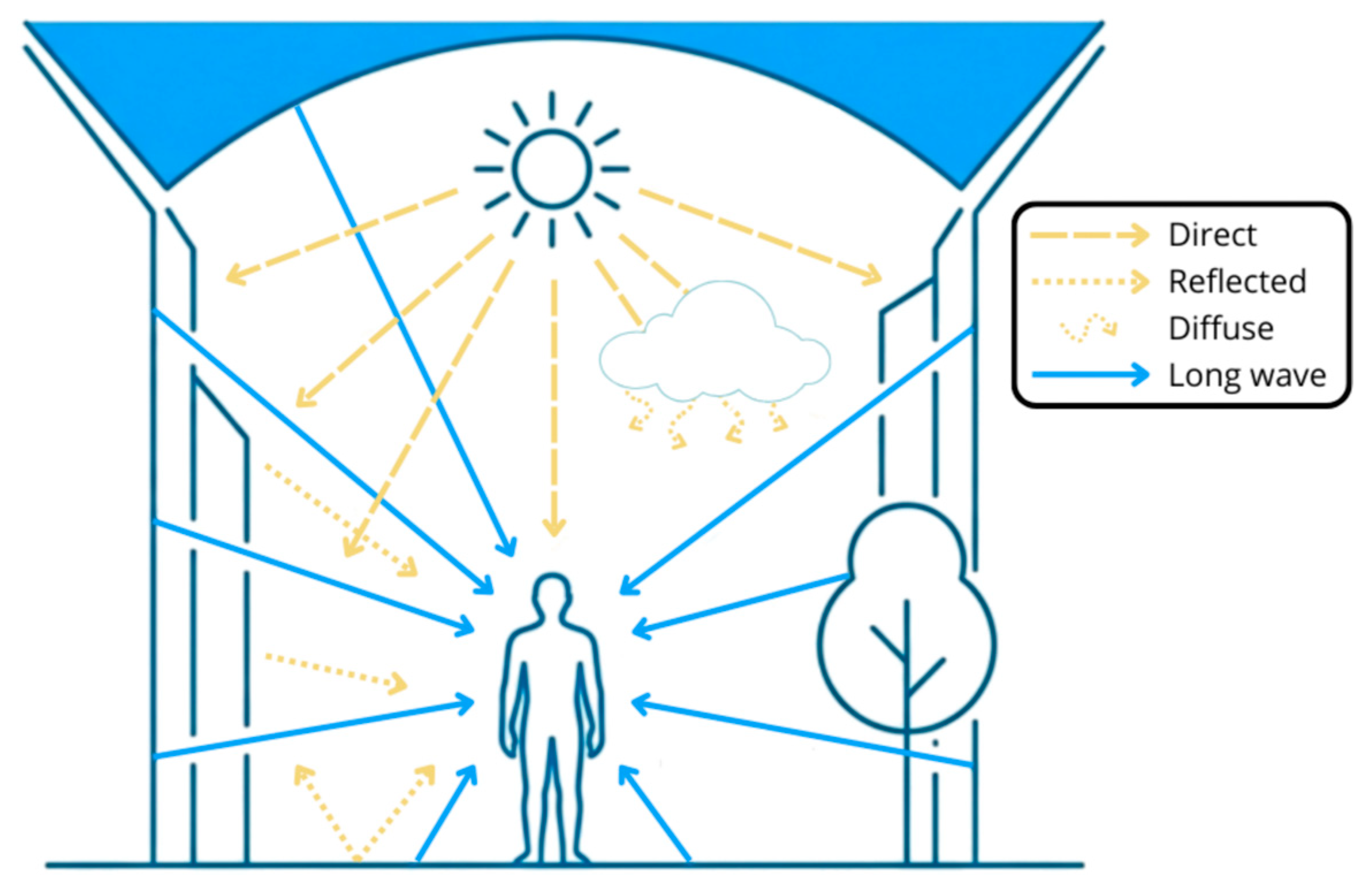
The left-hand side of Equation (1) represents the total long-wave radiation emitted by the human body to achieve equilibrium with an ideal, isothermal enclosure. σ = 5.67 · 10 8   W m 2 K 4 is the Stefan–Boltzmann constant, ϵ b o d y = 0.97 is the average emissivity of human body. The two components on the right-hand side of Equation (1) represent the short and long-wave radiation, e.g., the total amount of radiation received by the human body. The short-wave component, α k I s w , quantifies the solar radiation adsorbed by the subject, where α k is the absorption coefficient for a standard pedestrian and I s w is the total incident solar radiation on the subject. The term i F i ϵ i T i 4 accounts for the long-wave radiation, received from surrounding urban surfaces, including building facades, ground materials, vegetation, and the sky vault. Each surface i is characterized by its emissivity ϵ i and a surface temperature Ti which is dynamically computed based on the local configuration and solar exposure, due to the inertia of different materials. The relative influence of these surfaces on the pedestrian, is weighted by the view factors Fi. Figure 1 shows the schematic view of the described balance (Equation (1)).
The geometric coefficients Fi represent the fraction of the pedestrian’s field of view occupied by each environmental component, effectively linking the urban morphology—such as canyon narrowness or open spaces—to the thermal sensation.
Two parameters are defined to characterize the complexity of the urban morphology: the Sky View Factor (SVF) and the density of trees (gftrees), representing, respectively, the portion of sky viewed and the amount of arboreal vegetation surrounding the pedestrian. By exploiting these two parameters, the normalized view factors Fi can be defined as follows:
F g r o u n d = 0.5
F s k y = 0.5 · S V F · ( 1 τ t r e e s · g f t r e e s )
F w a l l = 0.5 · 1 S V F · 1 τ t r e e s · g f t r e e s
F v e g = 0.5 F w a l l F s k y
With this parametrization, it is assumed that the leaf cover of the trees is a screen in front of everything, which, therefore, dampens the portion of sky and buildings with a transmittance factor τ t r e e s . The assignment of a fixed value of 0.5 to the ground view factor (Fground) is firmly rooted in standard biometeorological practices for assessing pedestrian thermal comfort (e.g., ISO 7726 and VDI 3787 Part 2 [47,48]), which are structurally implemented in state-of-the-art benchmark models such as RayMan pro3.1, ENVI-met 5.8, and SOLWEIG/UMEP 4.4. In this framework, the pedestrian is approximated as a vertically oriented cylinder or sphere at a reference height of 1.1 m. Consequently, on a flat surface, the lower hemisphere of the subject’s radiant field of view is entirely occupied by the ground (Fground = 0.5).
Notably, this geometric relation remains robust even in densely built urban canyons, as surrounding obstructions primarily affect the upper hemisphere—redistributing the view factors between the sky and vertical walls—without significantly altering the pedestrian’s view of the street surface.
However, it is important to note that this assumption is theoretical. Inside highly complex urban topographies featuring slopes, staircases, or immediate low-level obstructions, the actual Fground may deviate from this theoretical constant.
Recent empirical analyses by Zhengrong Li et al. [49] have quantified the critical sensitivity of MRT to the ground view factor, demonstrating that a deviation of 0.1 in Fground can induce an MRT calculation error of up to 5 °C, and deviations as small as 0.01 can still shift the MRT by over 1 °C. While the constant 0.5 value provides a reliable baseline for the flat topographies simulated in this study, future iterations of the LUCIDiT framework will aim to implement a dynamically variable Fground. This could be achieved by incorporating a parameterized dependence on the SVF or high-resolution 3D morphological features [19], further enhancing the model’s accuracy in capturing the thermal nuances of complex urban terrains.
The longwave radiative exchange is modeled by summing the thermal emissions from four primary surfaces: sky, ground, building walls, and vegetation.
Surface temperatures are estimated using a simplified heat balance rather than full computational fluid dynamics. Following the approach suggested in [19], ground and wall temperatures are modeled as deviations from the air temperature:
T w a l l ( g r o u n d ) = T a i r + d T w a l l ( g r o u n d ) .  
However, to address the limitation of static coupling, we introduce a time-dependent radiative term that accounts for the thermal inertia of different urban materials. The surface temperature deviation is calculated as proportional to an inertial solar irradiance (Iinertial):
d T i = K i · S A F · I i n e r t i a l I m a x · 1 α i ,  
where α i is the albedo of the surface material i, Ki is a scaling coefficient [°C], Imax = 1000 Wm−2 a normalizing factor. This value is selected as it represents a widely accepted standard reference for peak Global Horizontal Irradiance (GHI) at sea level under clear sky conditions at medium low latitudes (exactly like the one that concerns Florence), aligning with the reference irradiance used in Standard Test Conditions (STC) for solar applications [50,51]. It effectively scales the radiative forcing for typical urban summer conditions in temperate climates.
In geographical regions characterized by high elevation, tropical latitudes, or extremely high atmospheric transparency, the actual solar irradiance can systematically exceed 1000 Wm−2 and the Imax parameter within the LUCIDiT framework can be adjusted to reflect the local climatological upper bounds to prevent underestimation of the thermal forcing.
SAF is the Solar Access Factor, a geometric proxy introduced to easy integrate the shading effect, defined as:
S A F = max 1 a · S d , S A F m i n ,
with a = 0.5 and SAFmin = 0.5. SAF depends directly form the shadow density (Sd).
This parameter, included in [0, 1], represents the amount of direct solar radiation shielded by buildings or trees. This is dynamically updated from the solar angle, projecting the shape of the obstructions onto the surface at height z = 1.5 m. Shadows generated by buildings give values of Sd = 1, while the shadow density from trees depends on specific vegetative parameter, the Leaf Area Index (LAI), and the Sun elevation β (the angle between the Sun’s rays and a horizontal plane), following a Beer–Lambert exponential decay [52]:
S d = 1 exp k e · L A I sin β ,  
with the attenuation factor ke = 0.6.
The term Iinertial is not the instantaneous solar radiation, but a historical convolution of the radiation that affects the surface. To simulate heat storage and release without solving differential equations, EWMA is employed [44]. This acts as a recursive low-pass filter on the radiation time series:
I i n e r t i a l t = γ · I g l o b a l t + 1 γ · I i n e r t i a l t 1 .
The decay factor γ ( 0 < γ 1 ), directly related to the thermal time constant τ , determines the thermal memory of the system.
Radiative contributions from the sun are obtained starting from the decomposition of GHI into direct and diffuse components using the semi-empirical model proposed by [53]. Based on solar elevation β and the clearness index, the model determines the diffusive fraction kd. Consequently, the Diffuse Horizontal Irradiance (DHI) and the Direct Normal Irradiance (DNI) are calculated as follows:
D H I = G H I · k d ,
D N I = G H I D H I s i n ( β ) .
For the walls, Iglobal = DNI e γ = 0.25 , corresponding to a value τ = 2 3 h. For the soil, a primary composition of two classes of different materials, asphalt and greenery is assumed. Greenery concentration is characterized using a density fraction gfground. The resulting temperature of the soil will be an average of the surface temperature deviation of the two material (obtained from Equation (7)) weighted by the gfground:
T g r o u n d = T a i r + 1 g f g r o u n d · d T a s p h a l t + g f g r o u n d · d T g r e e n e r y .
For this surface, the main assumption is: an incident solar radiation Iglobal = GHI, γ a s p h a l t = 0.25 , corresponding to a value τ = 5 6 h and γ g r o u n d = 0 . 8, corresponding to a value τ 1 h. The scaling factor Ki is chosen to represent the potential maximum temperature rise for the material under global solar exposure. Following the literature experimental/simulation evidence [54,55], a value of Kwall = 25 °C, and Kasphalt = 45 °C and Kground = 7 °C (otherwise until 18 °C for extreme limit conditions) is imposed. These values physically correspond to a maximum increase in surface temperatures with respect to the air temperatures of 15 °C, 30 °C, and 5 °C (otherwise until 15 °C), respectively.
The bifurcated choice for the Kground coefficient is introduced to distinguish between healthy, irrigated grass—where evapotranspiration has a significant impact on the adiabatic saturation effect of the air and therefore on local cooling, reducing surfaces’ warming—and the condition in which the herbaceous green cover is dry and/or subjected to water stress, and does not trigger cooling processes, thus reaching higher surface temperatures [56]. Unless explicitly specified, in this study, the greenery, all types of green cover, is considered healthy, both biophysically and structurally, and well-irrigated. Essentially, the European directives [57] on plant health and biosecurity are also taken into account, which require all plants (entire plants, fruit trees, lawns, and green cover, etc.) imported into the EU to be accompanied by a phytosanitary certificate (exemptions: bananas, coconuts, dates, pineapples, and durians, which are not easily direct introduced into urban areas, like Florence due to their climate, morphology, and hydrogeology).
Deep sky is modeled as a heat sink, with an apparent temperature derived from ambient air temperature adjusted by a cloud-cover proxy calculated from the diffuse fraction ratio:
T s k y = T a i r 12 · 1 D H I G H I .
In this, a maximum cooling effect up to 12 °C with respect to ambient temperatures can be assumed.
Vegetation is modeled as life system; indeed, trees temperature is evaluated taking in account the evapotranspiration effect of the vegetative system, modeled as a Penman–Monteith equation [45,46]. This model calculates the energy balance of the canopy by solving for the latent heat flux ( λ E ) and the sensible heat flux. The standard aerodynamic resistance (ra), which governs the heat and mass transfer is considered, estimating the water vapor mass as a function of wind speed and surface roughness, this last one parameterized as a constant (ra = 20 sm−1) [58]. This parameterization decouples the model from explicit wind speed field inputs, a climatic parameter that usually is mapped through urban canyon modeling with computationally expensive Computational Fluid Dynamics (CFD) simulations or dense sensor networks.
The canopy temperature is derived from the residual sensible heat flux after accounting for evapotranspiration:
T v e g = T a i r + R n λ · E · r a   ρ · C p     ,
where ρ · C P is the volumetric air heat capacity and R n is the net solar radiation, estimated as a balance between shortwave absorption (accounting for albedo α = 0.2 ) and a net longwave loss (assumed as average constant value −60 Wm−2).
The physiological regulation of transpiration is modeled via the canopy stomatal resistance (rs), which follows a multiplicative Jarvis-type approach [59]. This formulation accounts for the limiting factors of available solar energy and atmospheric demand:
r s = r s , m i n   f l i g h t · f V D P ,  
where rs,min represents the minimum stomatal resistance (set to 100 sm−1). The scaling functions flight and fVPD modulate stomatal aperture, based on GHI and Vapor Pressure Deficit (VDP), respectively, simulating the physiological closure of stomata during periods of low light or high evaporative demand.
For the short-wave component, the total solar flux Isw needs to be estimated. This is highly sensitive to the spatial distribution of shadows, which is modeled through a shadow density parameter (Sd).
The total shortwave flux (Isw) incident on the pedestrian aggregates four distinct contributions: direct beam radiation, diffuse sky radiation, and reflected radiation from both vertical walls and the horizontal ground:
I s w = I d i r + I d i f f + I r e f w a l l + I r e f g r o u n d .
The direct component is modulated by the projected area factor of the human body and the probability of shading, which is dynamically determined by the presence of buildings and vegetation:
I d i r = D N I · 1 S d · f p ,
where the term (1 − Sd) represents the pedestrian’s exposition to direct sunlight. This parameter is introduced to modulate the impact of direct beam radiation and differentiate the conditions of complete solar exposure from shaded areas. The parameter fp is the projected area factor, which accounts for the cylindrical geometry of the standing subject as a function of the Sun elevation β [60], neglecting the shadows produced by the 3D cylinder/person:
f p = 0.308 · cos β · 0.998 β 2 50000 .
The scattered radiation is weighted by the portion of sky observed by the pedestrian:
I d i f f = D H I · F s k y .
The reflected radiation contributions from the ground and walls are subsequently calculated by modulating the incident flux by the surface albedo and the specific view factors for the surface i = ground, wall:
I r e f ( i ) =   I i n c i d e n t ( i ) · S A F · α i · F i ,
where SAF is the surrounding sun factor defined as Equation (8), with a = 0.6 and SAFmin = 0.4. In this way it is assumed that when the pedestrian is in the shade, the surfaces from which it receives the reflected radiation are also placed in the shade, but with a variable portion of these remaining exposed to the sun.
The ground albedo is the average between the albedo of two main materials composing it, i.e., asphalt and greenery, weighted by the green fraction of the greenery gfground.
The incident horizontal solar radiation on the ground is GHI, i.e., I i n c i d e n t g r o u n d = GHI, the total radiation incident on vertical walls I i n c i d e n t ( w a l l ) must be explicitly derived.
The latter one is defined as the sum of the vertical component of the direct beam, diffuse sky radiation and the radiation reflected from the ground onto the walls:
I i n c i d e n t   ( w a l l ) =   I v e r i c a l _ d i r   +   I v e r i c a l _ d i f f   +   I v e r t i c a l _ r e f _ g r o u n d .
These vertical components are approximated by the following group of three similar equations:
I v e r i c a l _ d i r = 0.5 ·   D N I · cos β ,
I v e r i c a l _ d i f f = 0.5 · D H I ,
I v e r i c a l _ r e f _ g r o u n d = G H I · α g r o u n d · F g r o u n d .
The factor of 0.5 applied to the direct and diffuse vertical component, relies on the statistical assumption that within a random urban orientation, approximately half of the vertical surfaces are exposed to the sun while the other half are in shade.

2.2. Mapping and Implementation on Real Urban Scenario

To demonstrate the applicability of LUCIDiT model on real data, a geospatial pipeline is developed to translate real urban geometries into the input feature of the model. This process integrates static georeferenced datasets with dynamic climatological series to generate all the inputs required by the model.
The mapping process utilizes OpenStreetMap (OSM) [61] and, where provided, municipal cadastral data to reconstruct the building footprints and their respective heights, which are essential for determining the local urban morphology. This geometric information is discretized into a high-resolution grid (typically 1 × 1 m), where each cell is treated as a potential pedestrian location. To optimize computational efficiency, static morphological features are precomputed for each grid cell.
The SVF, as obstruction made from the buildings, is derived using a simplify sector-based ray-tracing algorithm that scans the surrounding environment to identify obstruction angles caused by urban elements, integrating these into a view factor representing the visible sky dome. Simultaneously, vegetation density is modeled as a continuous field rather than a binary classification; an inverse distance weighting approach smooths the discrete presence of trees and grass to assign effective green fraction values (gftrees, gfground) to each cell, based on the proximity factor.
Meteorological boundary conditions are established using data from meteorological station, or, if not provided, Typical Weather Year (TWY) datasets retrieved via the PVGIS database [62]. For every simulation time step, the pipeline extracts air temperature Tair, relative humidity RH and GHI while solving the solar geometry to determine Sun elevation β . These dynamic variables drive the shadow-casting algorithm, which projects the footprints of buildings and trees onto the ground plane based on the instantaneous solar position.
The resulting shadow polygons are intersected with the grid centroids to compute the Shadow density Sd. Building shadows are modeled as binary obstructions blocking direct radiation, whereas vegetation shadows are treated probabilistically; within tree shadows, intensity follows an exponential decay function of the local green fraction gftrees and LAI to simulate canopy transmittance (Equation (9)).
Finally, surface albedos are assigned, with ground albedo dynamically interpolated between vegetative and asphalt reference values. This procedure yields a complete, time-resolved dataset for the entire domain, serving as the input for LUCIDiT model to generate high-resolution MRT maps.
The use of LUCIDiT model allows for generating a spatially continuous map of the MRT in a fraction of the time required by traditional CFD or ray-tracing simulations. This efficiency enables the rapid transition from a static urban representation, to a dynamic UDT capable of simulating various microclimatic conditions and using all easily accessible and available data/information in an integrated approach.

3. The Case Study

To ensure the reliability of the surrogate model, a validation phase is conducted by comparing the model’s predictions against experimental data collected during a field measurements campaign in an urban area of Florence (Firenze Nova district) and, consequently with UMEP, an open source tool for QGIS (v.3.44.7 Solothurm), a validated model from [33].
The experimental investigation has been carried out for the EU LIFE-ESCAPOS project implementation, on a representative and significant urban area, from the UHI formation point of view, used as a primary pilot site.
The proposed method lays the foundation for one possible approach to the Dynamic Control Volume (DCV) modeling, a thermodynamic approach specifically designed for the multi-scale analysis of urban energy and entropy flows [63]. The studied area (43°48′ 23.472″ N, 11°13′ 40″ E; elevation 50 m a.s.l.) covers approximately 0.15 km2 and is characterized by a heterogeneous urban fabric, which includes varying building heights and vegetation densities, providing a challenging benchmark for the UDT.
The core of this urban site is Lippi’s Garden, an expansive green space featuring a different arboreal canopy. Existing greenery includes mature specimens (exceeding 20 m in height) and younger trees. This green infrastructure is integrated into a residential context, where building geometries generate urban canyon effects (buildings’ height does not exceed 25 m due to the presence of the airport site few kilometers away).
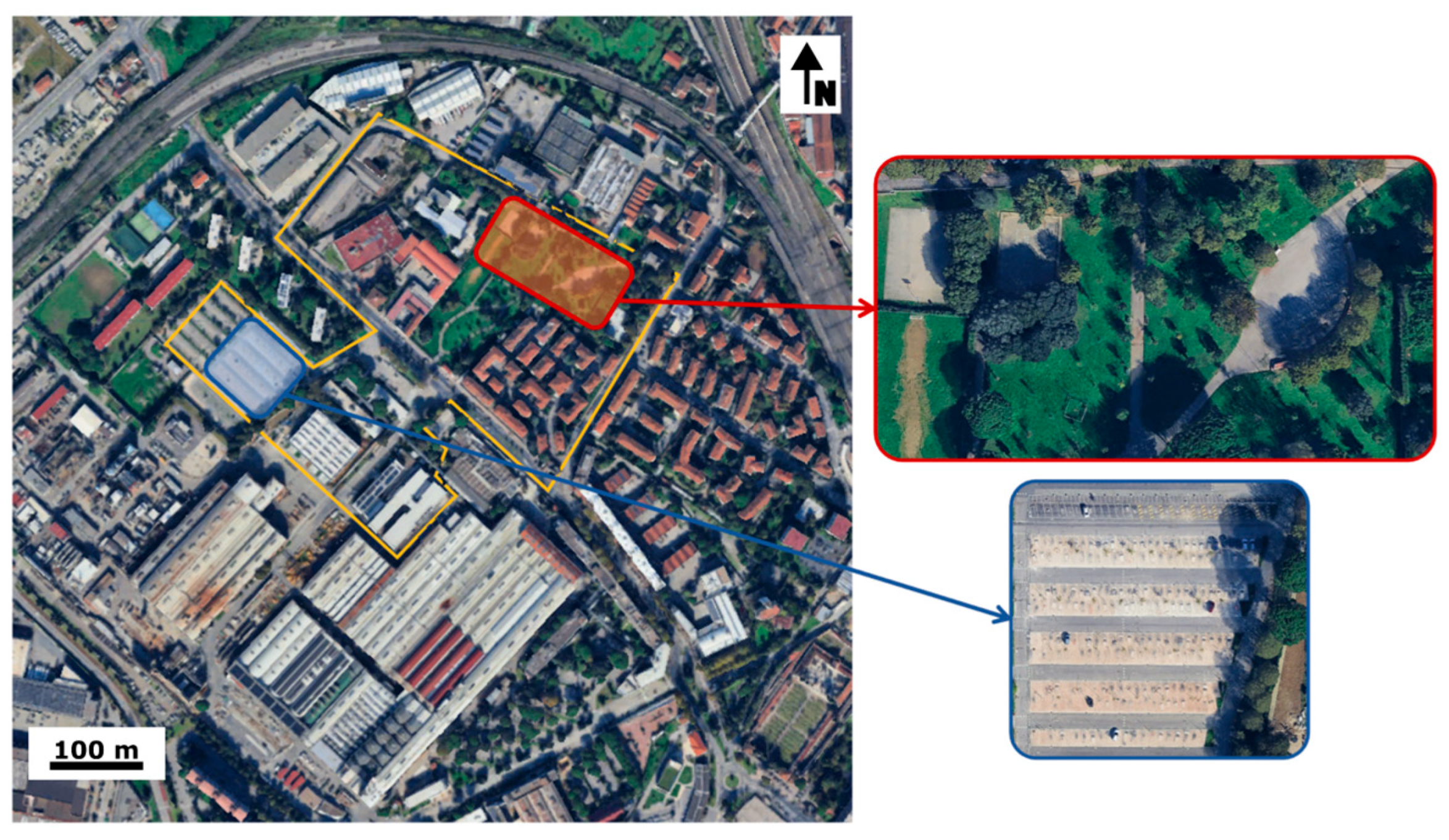
The district is further characterized by the presence of a nursery school in the north-western sector and a large industrial facility to the south-west (Figure 2).
Due to its geographical location, Florence occupies a transitional zone between a humid subtropical (Cfa) and a hot-summer Mediterranean (Csa) climate [64,65]. The region is characterized by temperate, humid winters and hot, often sultry summers frequently marked by convective phenomena. Long-term meteorological records (1991–2020) provided by LAMMA Consortium [66] indicate an annual mean temperature of 15.5 °C, which rises to a seasonal average of 24.5 °C during the summer months. Historical temperature extremes for the city range from a minimum of −10.2 °C to a maximum of 41.3 °C. Relative humidity typically fluctuates around 70%, peaking at 80% in winter and reaching its minimum average (approx. 65%) in July. Prevailing winter winds are predominantly south-westerly (SW), with average velocities ranging between 10–12 km/h.
In the first subsection we report the results obtained from the validation of LUCIDiT model with the data obtained from the drone measurement, in the second the comparison between LUCIDiT and UMEP models.

3.1. LICIDiT vs. Drone

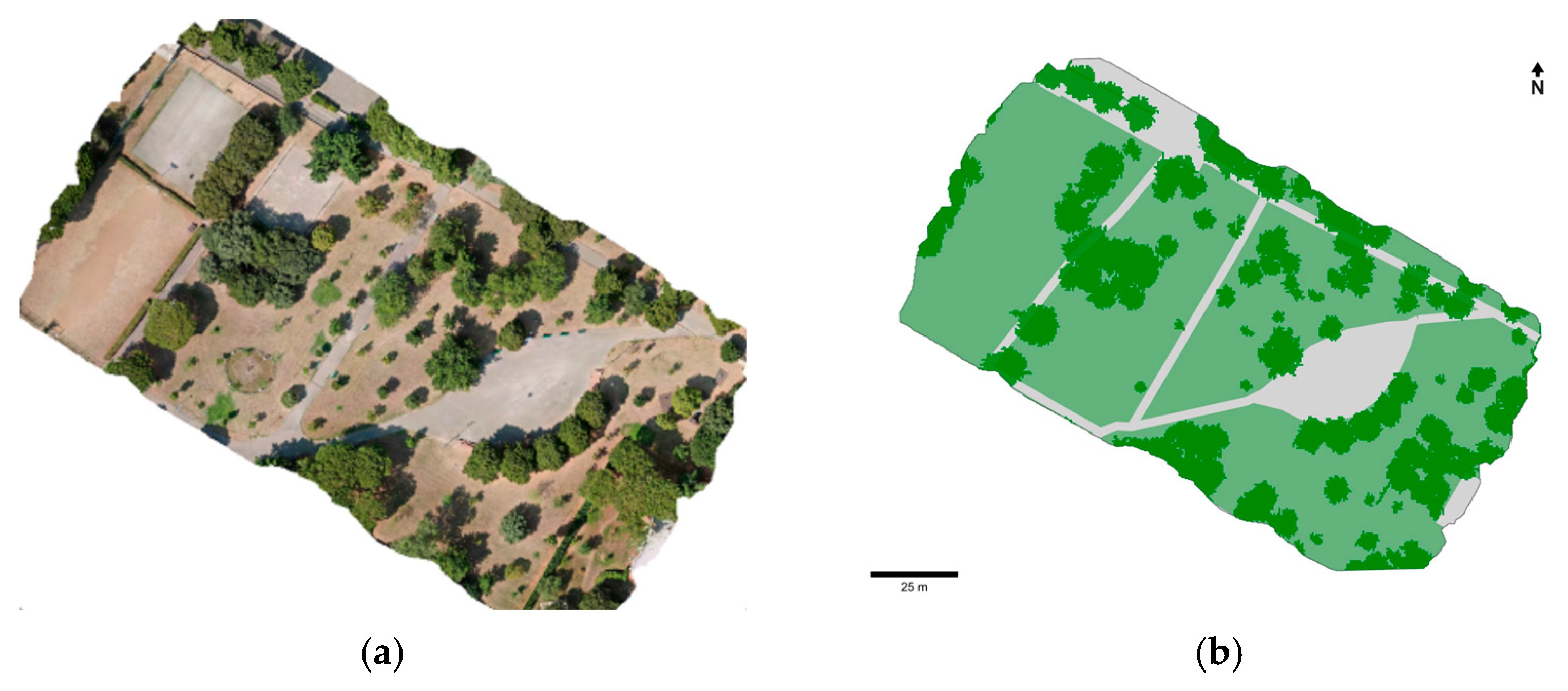
The validation of the surrogate model in a real-world operational context, is obtained by means of model predictions compared against the high-resolution thermographic data, acquired for the Lippi’s Garden. The experimental campaign is carried out exploiting drone surveys techniques. In particular, the Unmanned Aerial System (UAS) is equipped with a gimbal-stabilized thermal sensor 13.5 mm focal length, spectral sensitivity in the 8–14 μm range). Data acquisition is carried out through automated flight missions, enabling high-resolution coverage thanks to the match of hundreds of georeferenced thermal and RGB frames, aiming at the generation of an overall ground surface temperature map across the study area (referred to a mission conducted on 12 August 2025). The data post-processing procedure and aggregation used, is that suggested in [67]. Figure 3 shows the area considered for the analysis, as RGB image obtained by processing the photographs provided by drone flights (Figure 3a), and the digital reconstruction derived with the previously presented pipeline (Figure 3b).
To map the surface radiosity detected by the drone into a Mean Radiant Temperature (MRTdrone), directly comparable with the model’s output, a simplified longwave radiation balance is applied. Specifically, the MRTdrone is derived by aggregating the radiative contributions from the surrounding environment—including sky, buildings, trees, greenery and ground—according to the fundamental relationship, as follows:
ϵ b o d y M R T d r o n e 4 = ϵ i F i T i .
In this formulation, the ground surface temperature (Tground) is directly derived from the drone measurements. The temperatures of trees and buildings are approximated as equal to the ambient air temperature. Although this assumption may seem broad and lax in relation to building facades, its impact is numerically and physically negligible in the investigated Lippi’s Garden scenario, where the geometric view factor of buildings (Fbuildings) approaches zero. The sky temperature (Tsky) is parameterized according to the previously defined physical model (Equation (14)).
Furthermore, constant emissivity values are assigned to the different radiating surfaces: 0.94 for the ground (representing an average between vegetation and asphalt), 0.80 for the effective sky vault, 0.97 for trees, 0.90 for walls, and 0.97 for the reference pedestrian body ( ϵ b o d y ). The view factors (Fi) are maintained consistent with those derived from the morphological analysis algorithm.
The surrogate model, driven by boundary meteorological variables acquired from a local weather station, is specifically tuned to emulate the actual surveyed site conditions by setting the ground thermal scaling factor to Kground = 18 °C, in agreement with the hypothesis made for the scale factor for dry grass. Complementing this thermal tuning, the surface albedos within the model, are explicitly calibrated to reflect the specific thermal conditions of the local materials during summer: the asphalt albedo is set to 0.15, representative of an aged, dry, and light-colored pavement, while the grass albedo is fixed to 0.26, typical of a dry, unirrigated lawn.
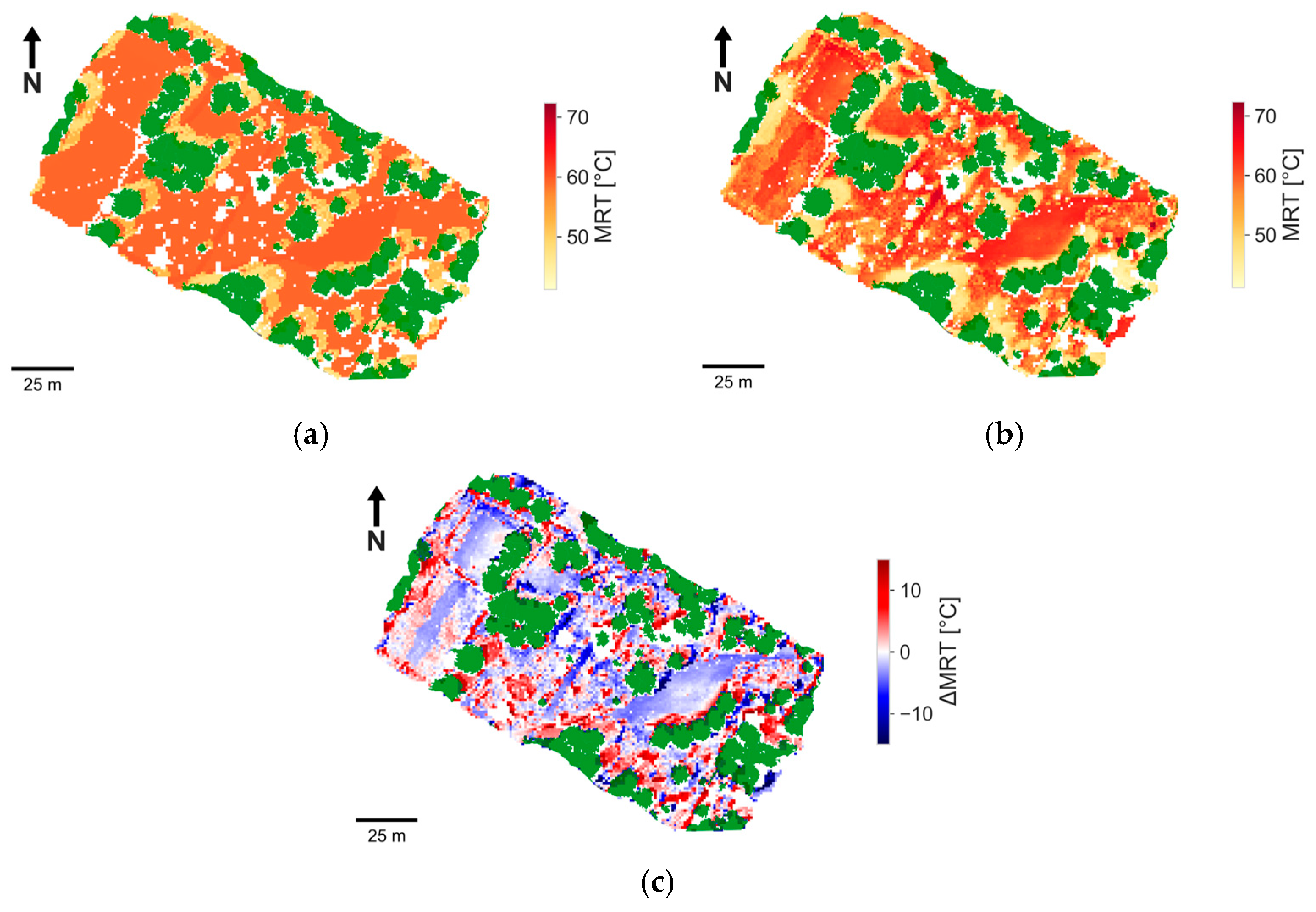
Figure 4 shows the spatial comparison between the model predictions (Figure 4a), the drone-derived MRT obtained using Equation (26) (Figure 4b), and the difference between the LUCIDiT prediction and the drone-derived estimation of MRT (Figure 4c). It can be noted that a good agreement is achieved between the modeled data and the measurement-derived results, with a mean error of −0.3 °C and a standard deviation of 5.6 °C, and a detailed observation of the spatial error distribution reveals two interesting points.
The first concerns a close inspection of the spatial map, which indicates that the drone-derived MRT values in shaded areas tend to be systematically lower than those predicted by the model. The second concerns the visual and statistical analysis, which highlights a broad simplification for the classification of different surfaces. Indeed, while the surrogate model successfully captures thermal gradients at the macroscale, its rigid categorization of horizontal surfaces into just two basic material classes—asphalt and dry grass—oversimplifies physical morphologies.
Consequently, the model generates thermal maps that do not take into account of highly intricate micro-variability of surface materials, localized variability of moisture levels, and subtle shading variations that are intrinsically present in the physical urban fabric, which instead are accurately captured by the drone’s high-resolution thermal sensors.

3.2. LUCIDiT vs. UMEP

The efficiency, performance, and specific behavioral traits of the LUCIDiT framework are evaluated by comparing its spatial and temporal predictions with those obtained with the established UMEP model. The area considered for comparison, the extent of which is approximately 38 ha, is shown in Figure 2. Meteorological inputs used for simulations are extracted from the TWY dataset.
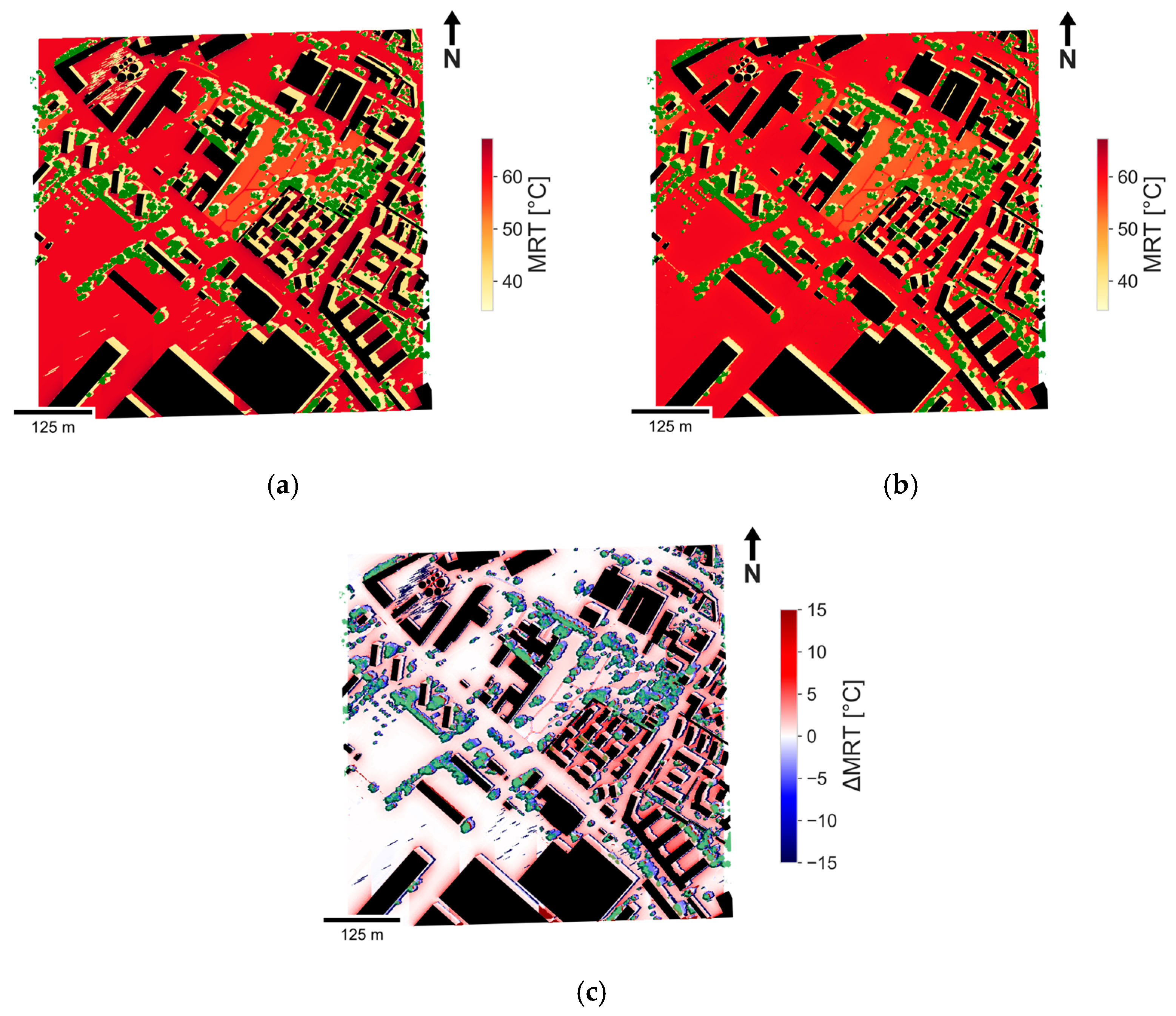
Figure 5 provides the spatial comparison between the two model predictions at 3 p.m. on August 12, the same day of the drone flight, with a maximum air temperature of 32.5 °C. In Figure 5a the MRT map predicted drone by LUCIDiT, in Figure 5b the UMEP prediction, and in Figure 5c the difference between our model and UMEP prediction.
The raw comparison yields a Mean Absolute Error (MAE) of 3.6 °C and a Mean Bias Error (MBE) of −0.9 °C.
However, this global metric is heavily skewed by highly localized peak deviations. To assess the baseline agreement of the radiative solvers across the bulk of the urban domain, a filtered metric is computed by excluding the absolute differences greater than 15 °C. When isolating the general domain from these specific boundary and microclimatic divergences—the physical reasons for which are detailed below—the baseline MAE drops to 1.5 °C with a positive bias of 0.7 °C.
LUCIDiT exhibits a wider variability in its spatial predictions, with extreme localized differences bounded within a range of [−20, 20] °C. These peak deviations do not indicate a systemic model failure but rather highlight fundamental differences in how the two models handle spatial discretization and applied thermodynamics.
Specifically, positive discrepancies (i.e., LUCIDiT predicting MRT values up to 20 °C higher than UMEP) are predominantly clustered along building perimeters and within narrow urban canyons. This is driven by two factors: firstly, the analytical parameterization of shortwave and longwave radiation trapping in LUCIDiT, which is strictly scaled by (1-SVF), resulting in pronounced thermal loads in deep geometries. Secondly, the boundary effects between LUCIDiT’s continuous vector raytracing and UMEP’s discrete raster grid generate sharp pixel-wise discrepancies along shadow terminators. A slight sub-pixel offset can result in one model computing full direct solar irradiance while the other computes deep shade, inherently generating an instantaneous ∆MRT of 15–20 °C.
Conversely, the extreme negative deviations (LUCIDiT predicting MRT up to 20 °C cooler) are strictly localized beneath and immediately surrounding vegetation canopies.
Because LUCIDiT treats trees as active thermodynamic entities—incorporating evapotranspiration cooling mechanisms—rather than mere passive optical filters for shortwave radiation, the longwave emission from the foliage is substantially lower.
This formulation is particularly important because yields a deep, localized microclimatic mitigation, highlighting the model’s high sensitivity to nature-based solutions.
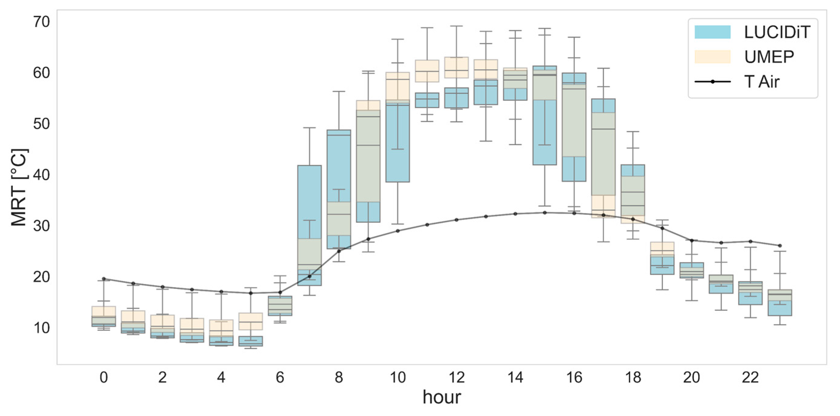
The temporal dynamics and the aforementioned divergences are effectively captured in the boxplots of Figure 6, which shows the hourly evolution across the entire day of August 12. The diurnal trends are accurately respected by LUCIDiT, capturing a broader daytime statistical dispersion of MRT extremes compared to UMEP, before converging tightly with UMEP’s baseline during the nighttime cooling phase.
Notably, the implementation of a delayed radiative forcing approach for surface temperature estimation, allows LUCIDiT to successfully replicate the nighttime cooling trends demonstrated by UMEP, which instead relies on explicitly solving transient heat exchange models for urban surfaces.
Consequently, LUCIDiT achieves comparable prognostic capabilities at a fraction of the computational cost: executed on equivalent hardware, the UMEP simulation required approximately 2.5 h, whereas the LUCIDiT pipeline converged in merely 90 s.

4. Results and Discussion

The previous sections (Section 3.1 and Section 3.2) demonstrate a fulfilling coherence between the LUCIDiT model and the local experimental results obtained by drone flights, such as between the same proposed method and the UMEP tool for QGIS.
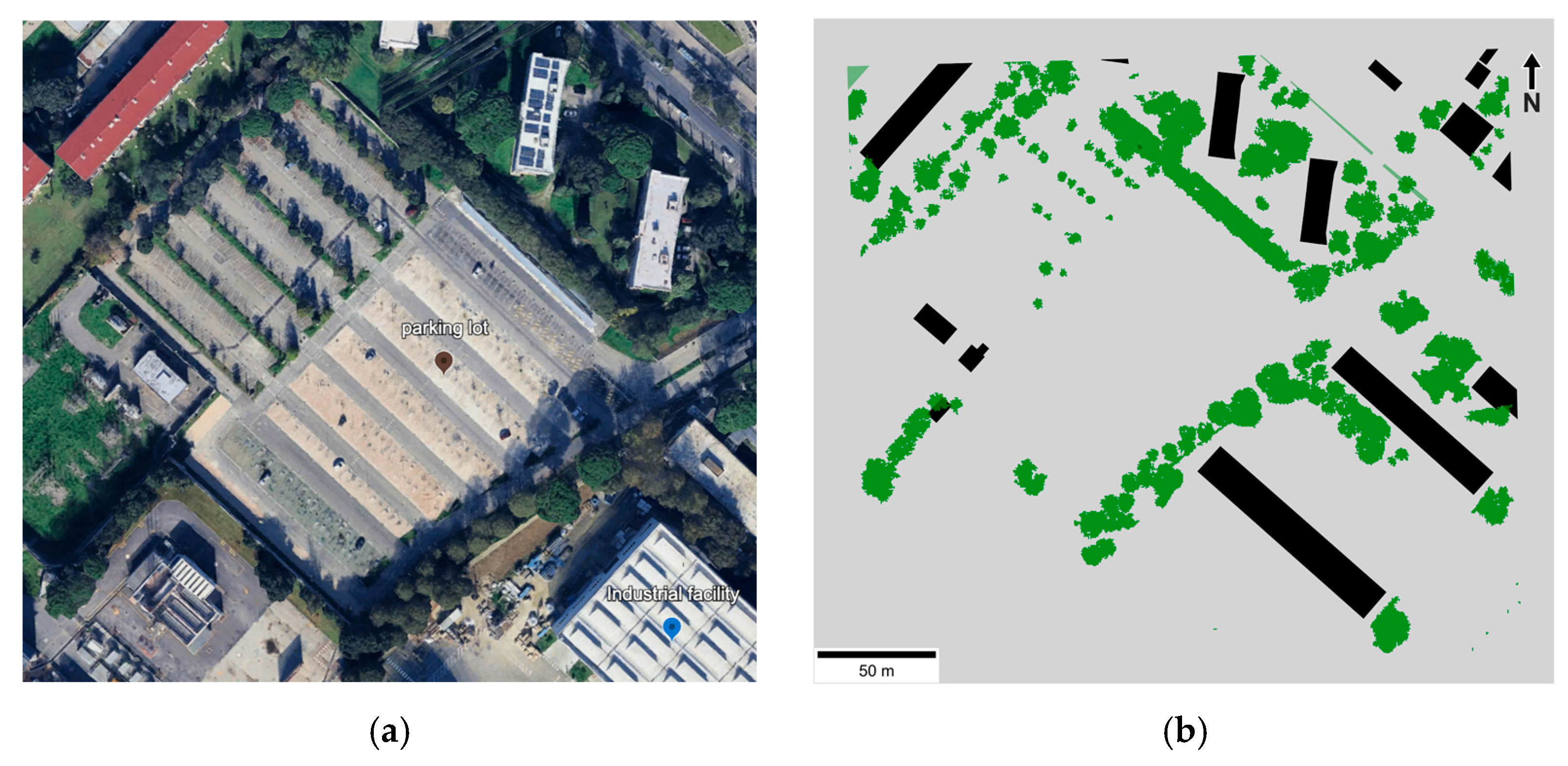
With the objective of testing the power and the capability of the model, LUCIDiT is applied in a specific zone of the pilot area for the impact assessment of some suitable urban interventions. The evaluation of the MRT is achieved in the area of the parking lot (Figure 7a in RGB and Figure 7b in the UDT) simulating: (i) the current layout, (ii) substitution of the asphalt with grass, and (iii) grass and planting of four new rows of trees (8 m height with a diameter of 5 m for each tree, the distance between the trees of each row is 8 m and the spacing among the rows is 16 m). These different solutions are analyzed in the extreme day of the TWY, which corresponds to 24 August 2023 (at 3 p.m.). The weather inputs for the simulation are Tair 37.7 °C, RH 21.7% and GHI 613 Wm−2.
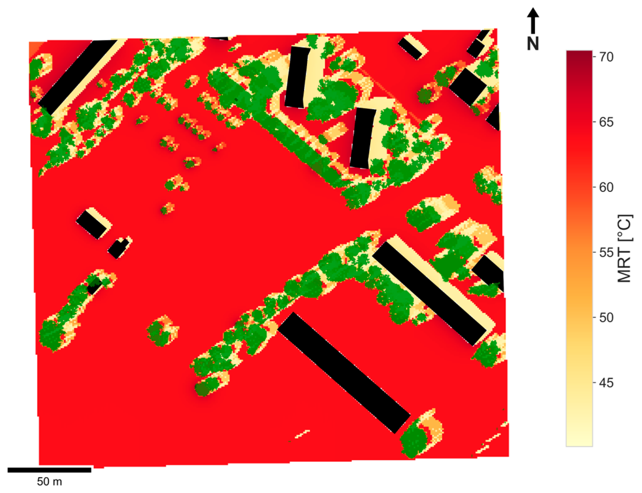
The current configuration exhibits a critical thermal scenario as shown in Figure 8: the parking lot is mainly paved with asphalt or dry ground and the radiative contributions, due to shadows’ absence, drive MRT to values between 60 °C and 65 °C (with an average value of 63 °C).
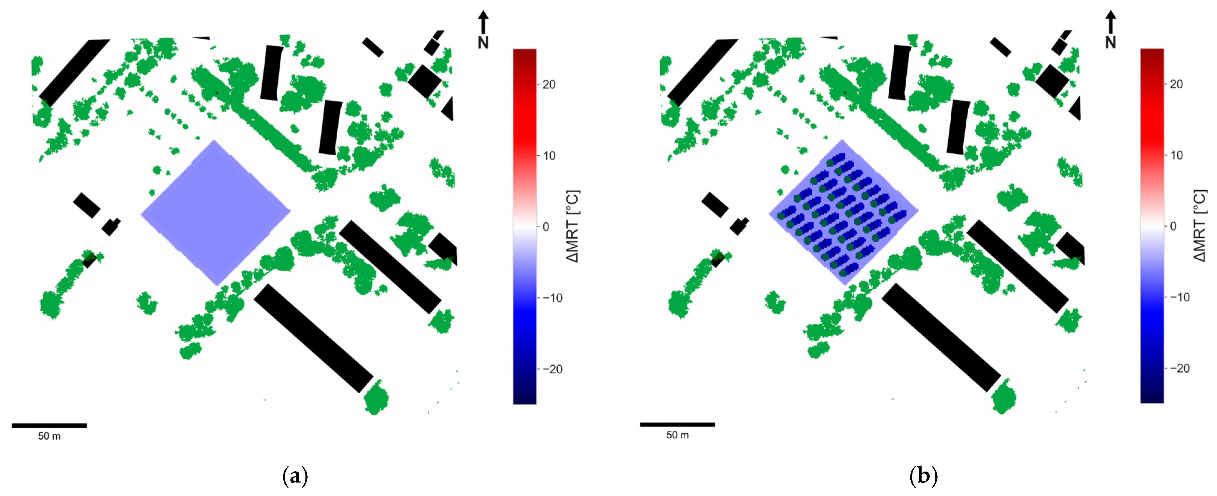
Building upon this framework, a vegetated lawn is modeled into the central portion of the parking area (of about 5000 m2). The changes of the MRT values are mapped as a difference ΔMRT, relative to the initial baseline configuration (Figure 9a).
Thanks to the increasing in the albedo and the scaling coefficient Kground (set at 7 °C for a well-irrigated healthy turfgrass), a drop in MRT is achieved for about 6 °C, even without integrating shade effects. Furthermore, the inclusion of trees results in a more significant decrease in MRT values. This enhancement is a direct consequence of the combined effect of evapotranspiration and shading, with the latter playing a crucial role in a local reduction in the radiant load on the ground. A maximum temperature reduction of 20 °C is observed in this case (Figure 9b). Again, LUCIDiT demonstrates high versatility and computational efficiency. Once the boundary conditions—including georeferencing, soil morphology, and material properties—are defined, each scenario requires approximately 10 s to generate high-resolution MRT maps.
A limitation observed during the spatial validation is the primary strict categorization of horizontal surfaces into broad macro-classes (e.g., standard asphalt versus dry grass), which provides a strong simplification of the real complex micro-variability of different materials. To address this, future development of LUCIDiT framework will be designed to incorporate an oriented much more granular, pixel-specific material classification—such as spatially variable different albedo, emissivity, and thermal admittance matrices derived from high-resolution satellite or multi-spectral drone imagery.
The authors believe that the integration of this level of granularity will not compromise the model “lean” computational advantage. Because LUCIDiT processes morphological and thermophysical properties as a priori input matrices, shifting from constant class-based values to heterogeneous spatial arrays will only slightly increase the initial memory allocation, while the execution time of the fundamental physical equations remain unaltered. Another simplification aspect of the proposed model is that it neglects fluid dynamic inside the urban context that which would require CFD simulations with greater computational costs. A CFD approach would undoubtedly enhance the method’s accuracy, by integrating local air-flow and velocity fields into the heat exchange analysis, but its application would involve greater complexity, both due to the multiplicity of necessary data required and to slow solutions due to the multi-physics coupling. Indeed, e.g., standard fixed meteorological stations are not suitable to provide the high-resolution data required for CFD-multi-physics modeling, needing to complex, hyper-local experimental data for its validation.
Furthermore, CFD-enhanced tools require highly specialized personnel, significant computational costs and resources, leading to substantially longer simulation times which would not allow the rapid-assessment by means of LUCIDiT.
In particular, convective heat exchange phenomena at the urban scale becomes significant when natural convection occurs in turbulent flow regimes, such as long, straight avenues aligned with prevailing winds (wind channels) or narrow high-rise streets. In these specific geometries, LUCIDiT will systematically underestimate convective cooling, leading to a conservative overestimation of surface temperatures and MRT. Conversely, in highly complex, deep, and with air stagnant and/or corto-circuit phenomena canyon geometries (e.g., narrow historical alleys), the lack of air mixing might lead to an underestimation of the perceived thermal stress.
In the investigated case, used for LUCIDiT application, hyperlocal air motion is mainly induced by very low mean air velocity values, ensuring that the radiative heat exchange is strong and prevalent. Indeed, the real measured thermal conditions show high external air temperatures, high material surface temperatures, and an average air velocity never exceeding 2 ms−1, that is a value usually associated to convection in turbulent flow regimes and modeled with CFD simulations [68,69].

5. Conclusions

This research proposes a novel methodology, based on LUCIDiT, for the dynamic assessment of MRT at the urban scale. Grounded in applied physics and thermodynamics, the algorithm effectively quantifies radiative heat exchange and the microclimatic influence of different materials of built-up and green areas. By bypassing computationally heavy explicit solvers, LUCIDiT drastically reduces execution times while maintaining high reliability—as demonstrated through validation against experimental drone data and established benchmark models like UMEP. The minimal requirements for input data—which in many cases are already readily accessible through modern open-source repositories—makes the tool operational for non-expert users, such as urban planners, municipal authorities, and various stakeholders.
The potential and effectiveness of LUCIDiT are further supported and corroborated by the results of the sensitivity analysis (Appendix A), which confirm the expected thermodynamic behaviors: an exponential cooling effect associated with increasing the LAI (consistent with the Lambert-Beer law) and the linear, yet distinct, impacts of ground and wall albedos. While these parameters act as independent design variables that can be actively modified for climate mitigation, intrinsic thermal properties—such as the thermal scaling coefficient (Ki) and time decay constant (γ)—were intentionally maintained as empirical “thermal footprints” to preserve physical realism. Arbitrarily modifying them would be mathematically equivalent to simulating the properties of fictitious, non-existent materials. However, a theoretical exploration of these parameters presents a highly valuable future prospect for advanced materials engineering, particularly for assessing the microclimatic impact of advanced next-generation urban surfaces with customized thermal inertia.
Future perspectives for LUCIDiT involve the development of a platform that, starting from local urban data to global databases on urban morphology (such as the Global Building Atlas [70]), facilitates extensive studies on urban comfort and design of effective, integrated climate adaptation interventions and strategies to mitigate UHIs across multiple scales, from local neighborhoods to global urban assessments. Moreover, additional intensive drone flight missions will be designed with a view to developing the method for the real radiative phenomena measurements, in several areas of the city, more densely built-up and with different environmental morphology, aiming at capillary validation of the model in contexts where the built-up is more predominant and/or strictly combined greenery and NBs.
The authors are currently investigating the application of their proposed tool to generate extensive datasets for training ML algorithms. This studied approach, aims to identify large-scale statistical correlations—while maintaining a rigorous link to the physics and thermodynamics of the underlying phenomena—to further accelerate outdoor thermal comfort assessment in urban environments.
Ultimately, LUCIDiT effectively bridges the gap between explicit 3D microclimatic modeling and computational efficiency. By providing a versatile, upgradeable, and fast framework for MRT evaluation, it empowers the implementation of intelligent UDTs, enabling rapid “what-if” scenario testing and the immediate comparison of climate adaptation strategies across different urban morphologies and climatic conditions, making it an effective and attractive tool for planners and decision-makers.

Author Contributions

M.B.; Writing, Methodology, Investigation, Validation, Software, Data curation; G.P.; Writing, Methodology, Investigation, Validation, Software, Data curation; C.B.; Writing, Review and Editing, Supervision, Funding Acquisition, Conceptualization. All authors have read and agreed to the published version of the manuscript.

Funding

This work was supported by the EU Project, LIFE Energy + LIFE Climate—Project 101157553-LIFE23-CCA-IT-LIFE ESCAPOS “Environmental energy for Strategic CApillary urban POlicieS”, funded by the European Union.

Institutional Review Board Statement

Not applicable.

Informed Consent Statement

Not applicable.

Data Availability Statement

The original contributions presented in this study are included in the article. Further inquiries can be directed to the corresponding author.

Conflicts of Interest

The authors declare no conflicts of interest and that they have no competing financial interests or personal relationships that could have appeared to influence the work reported in this paper.

Abbreviations

The following abbreviations are used in this manuscript:
CFDComputational fluid dynamics
DCVDynamical control volume
DHIDiffuse horizontal irradiance [Wm−2]
DNIDirect normal irradiance [Wm−2]
DNNDeep neural network
EWMAExponential weighted moving average
EUEuropean union
GHIGlobal horizontal irradiance [Wm−2]
GWGlobal warming
LAILeaf area index [-]
LSTLand surface temperature
LUCIDiTLean urban comfort intelligent digital twin
MAEMean absolute error
MBEMean bias error
MLMachine learning
MRTMean radiant temperature [°C]
NBSNature-based solutions
OSMOpenStreetMap
PETPhysiological environmental temperature [°C]
PIMLPhysics-informed machine learning
PVGISPhotovoltaic geographical information system
RHRelative humidity [%]
SAFSolar access factor [-]
SHAPShapley additive explaining
SVFSky view factor [-]
STCStandard test conditions for solar applications
TWYTypical weather year
UASUnmanned aerial system
UDIUrban digital twin
UHIUrban Heat Islands
UMEPUrban multi-scale environmental predictor
UTCIUniversal thermal climate index [°C]
VDPVapor pressure deficit [Pa]
Albedo [-]
βSun elevation [°]
γDecay factor of EWMA [-]
ϵEmissivity [-]
λLatent heat of vaporization [Jkg−1]
ρDensity [Kg m−3]
σStefan Boltzmann constant [Wm−2K−4]
τThermal time constant [s−1]
τtreesTree transmittance [-]
aDispersion coefficient of SAF [-]
CpSpecific heat [Jkg−1]
EEvapotranspiration rate [kgm−2s−1]
FiView factor [-]
flightLight scaling function of stomatal aperture [-]
fpProjected area factor [-]
fVDFEvaporation scaling function of stomatal aperture [-]
IdirDirect irradiance on pedestrian [Wm−2]
IdiffDiffuse irradiance on pedestrian [Wm−2]
IincidentIncident solar irradiance on surface [Wm−2]
IinertialInertial solar irradiance [Wm−2]
ImaxMaximum reference irradiance [Wm−2]
IrefReflected irradiance from surface on pedestrian [Wm−2]
IswShort wave irradiance on pedestrian [Wm−2]
Ivertical_dirDirect irradiance on vertical surface [Wm−2]
Ivertical_diffDiffuse irradiance on vertical surface [Wm−2]
Ivertical_ref_groundReflected irradiance from ground on vertical surface [Wm−2]
kdDiffusive fraction [-]
keAttenuation factor [-]
KiScaling coefficient of surface [°C]
gftreesTrees density [-]
gfgroundGreenery density [-]
raAerodynamic resistance [sm−1]
RnNet solar radiation on tree [Wm−2]
rsStomatal resistance [sm−1]
SdShadow density [-]
TairAir temperature [°C]
TiSurface temperature [°C]

Appendix A. Sensitivity Analysis

To evaluate the impact of the key parameters included in the modeling framework, a sensitivity analysis is performed on the Leaf Area Index (LAI) and the albedo of both the ground and the walls. The main aim is to assess how these parameters’ variation, affect the Mean Radiant Temperature (MRT) predicted by the model.
For a straightforward evaluation, all baseline model parameters are kept constant while the specific parameters selected for the sensitivity analysis are individually varied, calculating the resulting MRT values at strategic locations of interest.
Specifically, to evaluate the impact of the LAI, a location directly beneath a tree canopy is selected to quantify how this parameter dictates the shadow density Sd (Equation (9)).
To assess the influence of the ground albedo, which alters both the ground surface temperature and the reflected shortwave radiation, a location in an open, fully sunlit space is chosen. This fact effectively minimizes the interference from vegetation and the canyoning effects of surrounding buildings. Finally, to evaluate the impact of the wall albedo, a location adjacent to a single wall, but situated in its shadow, is considered. This isolates the weight of the wall’s albedo on the MRT—primarily driven by longwave and reflected radiation—by removing the direct radiative effects of the sunlit ground and surrounding vegetation.
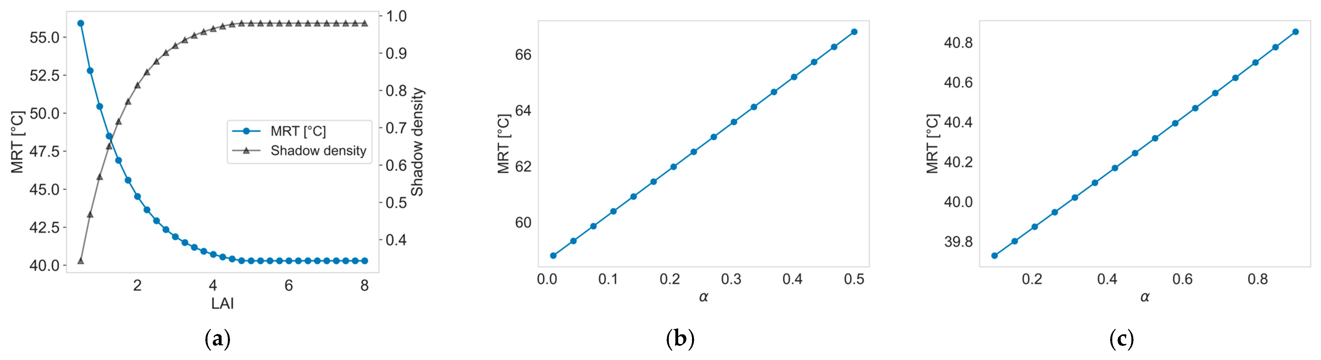
The obtained results are provided in Figure A1. Specifically, Figure A1a shows the sensitivity analysis for the LAI, Figure A1b for the ground albedo, and Figure A1c for the wall albedo.
Figure A1. Sensitivity analysis to quantify the impact of LAI (a), soil albedo (b), and wall albedo (c) on MRT predictions.
Atmosphere 17 00305 g0a1
It can be noted that increasing the LAI from values corresponding to bare trees (LAI = 0.5) to very dense canopies (LAI = 8), causes the MRT to decrease exponentially. This behavior consistently follows the increase in shadow density, also shown in Figure A1, which is modeled with a decreasing exponential trend according to the Lambert–Beer law (Equation (9)).
Conversely, the albedo variations result in a linear increase in the MRT. This trend emerges from the thermodynamic balance between the reflected shortwave radiation and the emitted longwave radiation; both of them depend linearly on the albedo parameter, but with opposite slopes. However, it is noteworthy that while an increase in the ground albedo from α = 0.05 to α = 0.5 leads to a substantial MRT increase on the order of ten degrees, the impact of the wall albedo is significantly less pronounced, resulting in an MRT increase on the order of only one degree.

References

  1. Huang, J.; Yu, H.; Guan, X.; Wang, G.; Guo, R. Accelerated dryland expansion under climate change. Nat. Clim. Change 2016, 6, 166–171. [Google Scholar] [CrossRef] [Scilit]
  2. Yuan, W.; Zheng, Y.; Piao, S.; Ciais, P.; Lombardozzi, D.; Wang, Y.; Ryu, Y.; Chen, G.; Dong, W.; Hu, Z.; et al. Increased Atmospheric Vapor Pressure Deficit Reduces Global Vegetation Growth. Sci. Adv. 2019, 5, eaax1396. [Google Scholar] [CrossRef] [Scilit] [PubMed]
  3. Hugonnet, R.; McNabb, R.; Berthier, E.; Menounos, B.; Nuth, C.; Girod, L.; Farinotti, D.; Huss, M.; Dussaillant, I.; Brun, F.; et al. Accelerated Global Glacier Mass Loss in the Early Twenty-First Century. Nature 2021, 592, 726–731. [Google Scholar] [CrossRef] [Scilit]
  4. Johnson, C.N.; Balmford, A.; Brook, B.W.; Buettel, J.C.; Galetti, M.; Guangchun, L.; Wilmshurst, J.M. Biodiversity Losses and Conservation Responses in the Anthropocene. Science 2017, 356, 270–275. [Google Scholar] [CrossRef] [Scilit]
  5. Díaz, S.; Settele, J.; Brondízio, E.S.; Ngo, H.T.; Agard, J.; Arneth, A.; Balvanera, P.; Brauman, K.A.; Butchart, S.H.M.; Chan, K.M.A.; et al. Pervasive Human-Driven Decline of Life on Earth Points to the Need for Transformative Change. Science 2019, 366, eaax3100. [Google Scholar] [CrossRef] [Scilit]
  6. Intergovernmental Panel On Climate Change (Ipcc). Climate Change 2021—The Physical Science Basis: Working Group I Contribution to the Sixth Assessment Report of the Intergovernmental Panel on Climate Change, 1st ed.; Cambridge University Press: Cambridge, UK, 2023. [Google Scholar]
  7. Diffenbaugh, N.S.; Singh, D.; Mankin, J.S.; Horton, D.E.; Swain, D.L.; Touma, D.; Charland, A.; Liu, Y.; Haugen, M.; Tsiang, M.; et al. Quantifying the Influence of Global Warming on Unprecedented Extreme Climate Events. Proc. Natl. Acad. Sci. USA 2017, 114, 4881–4886. [Google Scholar] [CrossRef] [Scilit]
  8. Mora, C.; McKenzie, T.; Gaw, I.M.; Dean, J.M.; Von Hammerstein, H.; Knudson, T.A.; Setter, R.O.; Smith, C.Z.; Webster, K.M.; Patz, J.A.; et al. Over Half of Known Human Pathogenic Diseases Can Be Aggravated by Climate Change. Nat. Clim. Change 2022, 12, 869–875. [Google Scholar] [CrossRef] [Scilit]
  9. Vicedo-Cabrera, A.M.; Scovronick, N.; Sera, F.; Royé, D.; Schneider, R.; Tobias, A.; Astrom, C.; Guo, Y.; Honda, Y.; Hondula, D.M.; et al. The Burden of Heat-Related Mortality Attributable to Recent Human-Induced Climate Change. Nat. Clim. Change 2021, 11, 492–500. [Google Scholar] [CrossRef] [Scilit]
  10. Watts, N.; Adger, W.N.; Agnolucci, P.; Blackstock, J.; Byass, P.; Cai, W.; Chaytor, S.; Colbourn, T.; Collins, M.; Cooper, A.; et al. Health and Climate Change: Policy Responses to Protect Public Health. Lancet 2015, 386, 1861–1914. [Google Scholar] [CrossRef] [Scilit] [PubMed]
  11. Obradovich, N.; Migliorini, R.; Paulus, M.P.; Rahwan, I. Empirical Evidence of Mental Health Risks Posed by Climate Change. Proc. Natl. Acad. Sci. USA 2018, 115, 10953–10958. [Google Scholar] [CrossRef] [Scilit] [PubMed]
  12. Dunne, J.P.; Stouffer, R.J.; John, J.G. Reductions in Labour Capacity from Heat Stress under Climate Warming. Nat. Clim. Change 2013, 3, 563–566. [Google Scholar] [CrossRef] [Scilit]
  13. Chen, L.; Ng, E. Outdoor Thermal Comfort and Outdoor Activities: A Review of Research in the Past Decade. Cities 2012, 29, 118–125. [Google Scholar] [CrossRef] [Scilit]
  14. Sherwood, S.C.; Huber, M. An Adaptability Limit to Climate Change Due to Heat Stress. Proc. Natl. Acad. Sci. USA 2010, 107, 9552–9555. [Google Scholar] [CrossRef] [Scilit]
  15. Stewart, I.D.; Oke, T.R. Local Climate Zones for Urban Temperature Studies. Bull. Am. Meteorol. Soc. 2012, 93, 1879–1900. [Google Scholar] [CrossRef] [Scilit]
  16. Ghoniem, M.; Fahmy, A.; Kamel, T.M. Evaluating Urban Surface Materials: Albedo Optimization and Shading for Pedestrian Thermal Comfort in Hot-Arid Environments. Architecture 2025, 13, 4331–4352. [Google Scholar] [CrossRef] [Scilit]
  17. Yang, J.; Yang, Y.; Sun, D.; Jin, C.; Xiao, X. Influence of Urban Morphological Characteristics on Thermal Environment. Sustain. Cities Soc. 2021, 72, 103045. [Google Scholar] [CrossRef] [Scilit]
  18. Iamarino, M.; Beevers, S.; Grimmond, C.S.B. High-resolution (Space, Time) Anthropogenic Heat Emissions: London 1970–2025. Int. J. Climatol. 2012, 32, 1754–1767. [Google Scholar] [CrossRef] [Scilit]
  19. Santamouris, M. Recent Progress on Urban Overheating and Heat Island Research. Integrated Assessment of the Energy, Environmental, Vulnerability and Health Impact. Synergies with the Global Climate Change. Energy Build. 2020, 207, 109482. [Google Scholar] [CrossRef] [Scilit]
  20. Cui, S.; Wang, X.; Yang, X.; Hu, L.; Jiang, Z.; Feng, Z. Mapping Local Climate Zones in the Urban Environment: The Optimal Combination of Data Source and Classifier. Sensors 2022, 22, 6407. [Google Scholar] [CrossRef] [Scilit]
  21. Chen, J.; Dong, Z.; Shi, R.; Sun, G.; Guo, Y.; Peng, Z.; Deng, M.; Chen, K. Urban Multi-Scenario Land Use Optimization Simulation Considering Local Climate Zones. Remote Sens. 2024, 16, 4342. [Google Scholar] [CrossRef] [Scilit]
  22. Chen, C.Y.; Chuang, Y.H.; Chen, H.W.; Teng, C.-S. Optimizing Ecological Corridors for Urban Sustainability by Using Remote Sensing and Decision Modeling. Int. J. Environ. Sci. Technol. 2025, 22, 10013–10028. [Google Scholar] [CrossRef] [Scilit]
  23. Hu, M.; Ghorbany, S.; Yao, S.; Wang, C. Micro-Urban Heatmapping: A Multi-Modal and Multi-Temporal Data Collection Framework. Buildings 2024, 14, 2751. [Google Scholar] [CrossRef] [Scilit]
  24. Guan, S.; Chen, Y.; Wang, T.; Hu, H. Mitigating Urban Heat Island through Urban-Rural Transition Zone Landscape Configuration: Evaluation Based on an Interpretable Ensemble Machine Learning Framework. Sustain. Cities Soc. 2025, 123, 106272. [Google Scholar] [CrossRef] [Scilit]
  25. Henn, K.A.; Peduzzi, A. Surface Heat Monitoring with High-Resolution UAV Thermal Imaging: Assessing Accuracy and Applications in Urban Environments. Remote Sens. 2024, 16, 930. [Google Scholar] [CrossRef] [Scilit]
  26. Zhang, S.; Zhang, X.; Niu, D.; Fang, Z.; Chang, H.; Lin, Z. Physiological Equivalent Temperature-Based and Universal Thermal Climate Index-Based Adaptive-Rational Outdoor Thermal Comfort Models. Build. Environ. 2023, 228, 109900. [Google Scholar] [CrossRef] [Scilit]
  27. Sharmin, T.; Steemers, K.; Humphreys, M. Outdoor Thermal Comfort and Summer PET Range: A Field Study in Tropical City Dhaka. Energy Build. 2019, 198, 149–159. [Google Scholar] [CrossRef] [Scilit]
  28. Kicovic, D.; Vuckovic, D.; Markovic, D.; Jovic, S. Assessment of Visitors’ Thermal Comfort Based on Physiologically Equivalent Temperature in Open Urban Areas. Urban Clim. 2019, 28, 100466. [Google Scholar] [CrossRef] [Scilit]
  29. Höppe, P. The Physiological Equivalent Temperature–a Universal Index for the Biometeorological Assessment of the Thermal Environment. Int. J. Biometeorol. 1999, 43, 71–75. [Google Scholar] [CrossRef] [Scilit] [PubMed]
  30. Vanos, J.; Guzman-Echavarria, G.; Baldwin, J.W.; Bongers, C.; Ebi, K.L.; Jay, O. A Physiological Approach for Assessing Human Survivability and Liveability to Heat in a Changing Climate. Nat. Commun. 2023, 14, 7653. [Google Scholar] [CrossRef] [Scilit] [PubMed]
  31. Li, N.; Shu, H.; Sun, D. Human Thermal Comfort Indicator in High-Temperature Environments in Deep Mining. J. Saf. Sustain. 2025, 2, 134–141. [Google Scholar] [CrossRef] [Scilit]
  32. Lopez-Cabeza, V.P.; Videras-Rodriguez, M.; Gomez-Melgar, S. An Open-Source Urban Digital Twin for Enhancing Outdoor Thermal Comfort in the City of Huelva (Spain). Smart Cities 2025, 8, 160. [Google Scholar] [CrossRef] [Scilit]
  33. Lindberg, F.; Grimmond, C.S.B.; Gabey, A.; Huang, B.; Kent, C.W.; Sun, T.; Theeuwes, N.E.; Järvi, L.; Ward, H.C.; Capel-Timms, I.; et al. Urban Multi-Scale Environmental Predictor (UMEP): An Integrated Tool for City-Based Climate Services. Environ. Model. Softw. 2018, 99, 70–87. [Google Scholar] [CrossRef] [Scilit]
  34. Zhong, X.; Voogt, J.; Bailey, B.; Zhang, X.; Krayenhoff, E.S. Evaluating High-Resolution Mean Radiant Temperature within an Urban Street Canopy: Resolving Spatiotemporal Variations with LiDAR/Thermal Infrared Scanning and Data-Driven Simulation. Build. Environ. 2025, 287, 113819. [Google Scholar] [CrossRef] [Scilit]
  35. Zhu, S.; Yan, Y.; Zhao, B.; Wang, H. Assessing the Impact of Adjacent Urban Morphology on Street Temperature: A Multisource Analysis Using Random Forest and SHAP. Build. Environ. 2025, 267, 112326. [Google Scholar] [CrossRef] [Scilit]
  36. Conigliaro, E.; Monti, P.; Leuzzi, G.; Cantelli, A. A Three-Dimensional Urban Canopy Model for Mesoscale Atmospheric Simulations and Its Comparison with a Two-Dimensional Urban Canopy Model in an Idealized Case. Urban Clim. 2021, 37, 100831. [Google Scholar] [CrossRef] [Scilit]
  37. Tian, G.; Ma, Y.; Chen, Y.; Wan, M.; Chen, S. Impact of Urban Canopy Characteristics on Turbulence Dynamics: Insights from Large Eddy Simulation. Build. Environ. 2024, 250, 111183. [Google Scholar] [CrossRef] [Scilit]
  38. Nazarian, N.; Krayenhoff, E.S.; Martilli, A. A One-Dimensional Model of Turbulent Flow through “Urban” Canopies (MLUCM v2.0): Updates Based on Large-Eddy Simulation. Geosci. Model Dev. 2020, 13, 937–953. [Google Scholar] [CrossRef] [Scilit]
  39. Mateen, S.A.; Giometto, M.G.; Biswal, B.; Tapper, N.J.; Parlange, M.B. Large Eddy Simulation Based Evaluation of an Urban Canopy Model. Bound. Layer Meteorol. 2025, 191, 34. [Google Scholar] [CrossRef] [Scilit]
  40. Snaiki, R.; Merabtine, A. Recent Advances on Machine Learning Techniques for Urban Heat Island Applications: A Review and New Horizons. Sustain. Cities Soc. 2025, 134, 106943. [Google Scholar] [CrossRef] [Scilit]
  41. Briegel, F.; Wehrle, J.; Schindler, D.; Christen, A. High-Resolution Multi-Scaling of Outdoor Human Thermal Comfort and Its Intra-Urban Variability Based on Machine Learning. Geosci. Model Dev. 2024, 17, 1667–1688. [Google Scholar] [CrossRef] [Scilit]
  42. Jia, S.; Wang, Y.; Hien Wong, N.; Liang Tan, C.; Chen, S.; Weng, Q.; Ming Mak, C. Estimation of Mean Radiant Temperature across Diverse Outdoor Spaces: A Comparative Study of Different Modeling Approaches. Energy Build. 2024, 310, 114068. [Google Scholar] [CrossRef] [Scilit]
  43. Rashtian, Z.; Manesh, M.T.; Tahsildoost, M.; Zomorodian, Z.S. Data-Driven Real-Time Visualization of Urban Heat Islands Using Mean Radiant Temperature for Urban Design. Energy Build. 2025, 333, 115470. [Google Scholar] [CrossRef] [Scilit]
  44. Nicol, F.; Humphreys, M. Derivation of the Adaptive Equations for Thermal Comfort in Free-Running Buildings in European Standard EN15251. Build. Environ. 2010, 45, 11–17. [Google Scholar] [CrossRef] [Scilit]
  45. Monteith, J.L. Evaporation and the Environment. In Proceedings of the 19th Symposium of the Society for Experimental Biology; Cambridge University Press: New York, NY, USA, 1965. [Google Scholar]
  46. Grimmond, C.S.B.; Oke, T.R. An Evapotranspiration-interception Model for Urban Areas. Water Resour. Res. 1991, 27, 1739–1755. [Google Scholar] [CrossRef] [Scilit]
  47. ISO 7726:2025; Ergonomics of the Thermal Environment—Instruments for Measuring and Monitoring Physical Quantities. International Organization for Standardization (ISO): Geneva, Switzerland, 2025.
  48. VDI. VDI 3787-2; VDI 3787 Part 2: Human Biometeorological Assessment of Climate for Urban and Regional Planning. VDI: Verein Deutscher Ingenieure: Düsseldorf, Germany, 2008.
  49. Li, Z.; Feng, X.; Chen, W.; Fang, Z. Quantifying the Effect of Ground View Factor and Ground Temperature on Outdoor Mean Radiant Temperature. Sustain. Cities Soc. 2022, 84, 104030. [Google Scholar] [CrossRef] [Scilit]
  50. IEC 61215-1:2021; Terrestrial Photovoltaic (PV) Modules—Design Qualification and Type Approval—Part 1: Test Requirements. International Electrotechnical Commission (IEC): Geneva, Switzerland, 2021.
  51. IEC 60904-3:2019; Photovoltaic Devices—Part 3: Measurement Principles for Terrestrial Photovoltaic (PV) Solar Devices with Reference Spectral Irradiance Data. International Electrotechnical Commission (IEC): Geneva, Switzerland, 2019.
  52. Campbell, G.S.; Norman, J.M. An Introduction to Environmental Biophysics; Springer: New York, NY, USA, 1998. [Google Scholar]
  53. Erbs, D.G.; Klein, S.A.; Duffie, J.A. Estimation of the Diffuse Radiation Fraction for Hourly, Daily and Monthly-Average Global Radiation. Sol. Energy 1982, 28, 293–302. [Google Scholar] [CrossRef] [Scilit]
  54. Pomerantz, M.; Akbari, H.; Chen, A.; Taha, H.; Rosenfeld, A.H. Paving Materials for Heat Island Mitigation; Report LBL-38074; Lawrence Berkeley National Laboratory: Berkeley, CA, USA, 1997. [Google Scholar]
  55. Santamouris, M. Cooling the Cities—A Review of Reflective and Green Roof Mitigation Technologies to Fight Heat Island and Improve Comfort in Urban Environments. Sol. Energy 2014, 103, 682–703. [Google Scholar] [CrossRef] [Scilit]
  56. Santamouris, M. Using Cool Pavements as a Mitigation Strategy to Fight Urban Heat Island—A Review of the Actual Developments. Renew. Sustain. Energy Rev. 2013, 26, 224–240. [Google Scholar] [CrossRef] [Scilit]
  57. Regulation (EU) 2016/2031 of the European Parliament of the Council of 26 October 2016 on Protective Measures against Pests of Plants, Amending Regulations (EU) No 228/2013, (EU) No 652/2014 and (EU) No 1143/2014 of the European Parliament and of the Council and Repealing Council Directives 69/464/EEC, 74/647/EEC, 93/85/EEC, 98/57/EC, 2000/29/EC, 2006/91/EC and 2007/33/EC. Available online: https://eur-lex.europa.eu/eli/reg/2016/2031/oj (accessed on 14 March 2026).
  58. Jones, H.G. Plants and Microclimate: A Quantitative Approach to Environmental Plant Physiology; Cambridge University Press: Cambridge, UK, 2014. [Google Scholar]
  59. Jarvis, P. The Interpretation of the Variations in Leaf Water Potential and Stomatal Conductance Found in Canopies in the Field. Philos. Trans. R. Soc. Lond. B Biol. Sci. 1976, 273, 593–610. [Google Scholar] [CrossRef] [Scilit]
  60. Fanger, P.O. Thermal Comfort. Analysis and Applications in Environmental Engineering; CABI Digital Library: Leusden, The Netherlands, 1970. [Google Scholar]
  61. Open Street Map. Available online: https://Www.Openstreetmap.Org (accessed on 16 January 2026).
  62. Photovoltaic Geographical Information System (PVGIS). Available online: https://Joint-Research-Centre.Ec.Europa.Eu/Photovoltaic-Geographical-Information-System-Pvgis_en (accessed on 16 January 2026).
  63. Balocco, C.; Grazzini, G. Thermodynamic Parameters for Energy Sustainability of Urban Areas. Sol. Energy 2000, 69, 351–356. [Google Scholar] [CrossRef] [Scilit]
  64. Beck, H.E.; Zimmermann, N.E.; McVicar, T.R.; Vergopolan, N.; Berg, A.; Wood, E.F. Present and Future Köppen-Geiger Climate Classification Maps at 1-Km Resolution. Sci. Data 2018, 5, 180214. [Google Scholar] [CrossRef] [Scilit]
  65. Kottek, M.; Grieser, J.; Beck, C.; Rudolf, B.; Rubel, F. World Map of the Köppen-Geiger Climate Classification Updated. Meteorol. Z. 2006, 15, 259–263. [Google Scholar] [CrossRef] [Scilit] [PubMed]
  66. Consorzio LAMMA. Available online: https://Www.Lamma.Toscana.It/Clima-e-Energia/Climatologia/Clima-Firenze (accessed on 16 January 2026).
  67. Pierucci, G.; Baia, M.; Balocco, C. Urban Area Sustainability Analysis by Means of Integrated Microclimatic Measurement Techniques Combined with Thermal Comfort Modelling—A Pilot Project Application. Energies 2025, 19, 217. [Google Scholar] [CrossRef] [Scilit]
  68. Palyvos, J.A. A Survey of Wind Convection Coefficient Correlations for Building Envelope Energy Systems’ Modeling. Appl. Therm. Eng. 2008, 28, 801–808. [Google Scholar] [CrossRef] [Scilit]
  69. Defraeye, T.; Blocken, B.; Carmeliet, J. Convective Heat Transfer Coefficients for Exterior Building Surfaces: Existing Correlations and CFD Modelling. Energy Convers. Manag. 2011, 52, 512–522. [Google Scholar] [CrossRef] [Scilit]
  70. Zhu, X.X.; Chen, S.; Zhang, F.; Shi, Y.; Wang, Y. GlobalBuildingAtlas: An Open Global and Complete Dataset of Building Polygons, Heights and LoD1 3D Models. Earth Syst. Sci. Data 2025, 17, 6647–6668. [Google Scholar] [CrossRef] [Scilit]
Figure 1. Schematic view of contributions used in the urban energy balance. In yellow color shortwave contribute, dashed line for direct radiation, dotted line for reflected radiation and dashed curve for diffuse radiation. In blue color is the longwave contribution.
Atmosphere 17 00305 g001
Figure 2. Top view of the study area in the North–East part of Florence—Google Maps web version source (enclosed by yellow line). In particular: red rectangle identifies drone flight zone above the Lippi’s Garden, blue rectangle the parking lot where the LUCIDiT model can be applied for suitable regenerative future scenarios.
Atmosphere 17 00305 g002
Figure 3. The studied area by drone in RGB (a) and in virtual representation of UDT (b).
Atmosphere 17 00305 g003
Figure 4. MRT maps for the real data test area predicted by LUCIDiT (a), Drone measurement (b) and the difference between LUCIDiT and Drone estimation (c). Areas in green color indicate the trees obstruction.
Atmosphere 17 00305 g004
Figure 5. MRT maps for the models test area predicted by LUCIDiT (a), UMEP (b), and the difference between LUCIDiT and UMEP predictions (c). Black areas indicate buildings; green areas indicate the trees obstruction. The spatial domain is titled due to the latitude–longitude orientation.
Atmosphere 17 00305 g005
Figure 6. Comparison of MRT calculation by LUCIDiT and UMEP for the extreme day of the TWY.
Atmosphere 17 00305 g006
Figure 7. The area studied for different suitable solutions in RGB (a) and in the UDT (b). In the UDT images, buildings are in black, and trees in green color.
Atmosphere 17 00305 g007
Figure 8. MRT map for the parking lot in the existing scenario. Black areas identify buildings; green areas the trees obstruction. The spatial domain is titled due to the latitude–longitude orientation.
Atmosphere 17 00305 g008
Figure 9. Difference of MRT in respect to the initial scenario: (a) adding turfgrass and (b) adding turfgrass and trees. Grey areas indicate buildings, and green areas color the trees obstruction. The spatial domain is titled due to the latitude–longitude orientation.
Atmosphere 17 00305 g009
Disclaimer/Publisher’s Note: The statements, opinions and data contained in all publications are solely those of the individual author(s) and contributor(s) and not of MDPI and/or the editor(s). MDPI and/or the editor(s) disclaim responsibility for any injury to people or property resulting from any ideas, methods, instructions or products referred to in the content.