GLKC-Net: Group Large Kernel Convolution for Short-Range Precipitation Forecasting

Abstract

Accurate short-range precipitation prediction plays a crucial role in daily life and disaster mitigation. However, the existing methods often suffer from inefficient large-scale feature extraction, severe redundant information interference, and insufficient attention to the problem of imbalanced data distributions, leading to unsatisfactory performance. To address these issues, in this paper, we first propose a novel spatiotemporal module called Group Large Kernel Convolution (GLKC) and develop a short-range precipitation forecasting model based on it, GLKC-Net, using multiple meteorological variables. Specifically, we use decomposed large-kernel convolution to enhance the ability to understand large-scale atmospheric processes. Meanwhile, we introduce the group convolution and channel shuffle operator to control the fusion of channel-wise information, enabling efficient information exchange and reducing redundancy in the channel dimension with multiple variables. Furthermore, we treat the causes of poor model performance for extreme precipitation events with an imbalanced data distribution perspective and design a Multi-threshold Adaptive Loss function (MTA Loss). This function strengthens the model’s focus on high-threshold precipitation events that are inherently difficult to forecast, aiming to improve model performance for extreme events. Finally, forecasting experiments for validation were conducted over southwestern China using ERA5-Land and CMPAS datasets. The results demonstrate that our proposed method outperforms several existing approaches in terms of forecasting accuracy.

1. Introduction

Short-range precipitation prediction refers to the timely and accurate prediction of precipitation intensity and spatial distribution within a specific region over a lead time of 2 to 12 h [1]. This plays a vital role in disaster prevention, agricultural production, and urban management [2]. Due to the inherent chaotic nature of weather systems, which are always influenced by surrounding weather changes and the complex interactions among various meteorological variables, precipitation is difficult to forecast [3,4]. Therefore, capturing the dynamic evolution of large-scale spatial relationships and effectively modeling the complex interactions among multiple meteorological variables remain key challenges in precipitation forecasting research. Meanwhile, under the influence of global warming, the instability of the climate system continues to intensify, leading to frequent occurrences of extreme events, and the precipitation distribution exhibits significant spatiotemporal heterogeneity [5]. Consequently, it is also necessary to account for this spatiotemporal imbalance in precipitation patterns to better address the occurrence of extreme precipitation events.

Traditional precipitation forecasting is primarily based on numerical weather prediction (NWP), which simulates future atmospheric states by numerically solving a set of atmospheric motion equations based on thermodynamic and dynamic principles [2]. This approach, implemented through high-performance computing systems, demonstrates excellent physical consistency. However, numerical models suffer from the “spin-up” problem, and various physical variables require a period of dynamic adjustment to reach a stable state at model initialization, making it difficult to meet the time requirements of short-range forecasting [6]. Moreover, constructing such models demands substantial domain expertise and prior knowledge. Under computational constraints, it becomes difficult for physical equations to consistently and precisely represent atmospheric dynamics, which can lead to accuracy degradation [7]. Finally, as the volume of historical data spatiotemporal resolution demands of short-range precipitation both increase, the computational cost of NWP models will rapidly escalate to prohibitively expensive levels [8,9]; as a result, it often fails to fully leverage the potential value contained in the big data [10].

With the rapid development and widespread application of deep learning (DL) techniques, these methods have been increasingly introduced to atmospheric sciences, including climate prediction and weather forecasting. Unlike NWP models, DL-based models are primarily data-driven, learning changes in data distribution from vast historical datasets [11]. Once trained, these models can rapidly generate forecasts based on input samples, effectively addressing the timeliness issues associated with numerical models. At the same time, DL methods can autonomously identify and model nonlinear variations in weather systems, including unknown patterns, without relying on complex physical knowledge [12]. This simplifies the design process and enables direct end-to-end data mapping. Such approaches exhibit strong compatibility with various types of data, allowing for the effective utilization of large volumes of meteorological data. Compared with traditional NWP models, these methods offer significant advantages in terms of computational efficiency and inference speed while achieving comparable or even superior forecast accuracy. For example, MetNet v3 [13] has extended the lead time for high-resolution (1 km) short-range forecasts in United States to 24 h and can provide probabilistic forecasts every 2 min, outperforming established forecasting systems such as High-Resolution Rapid Refresh (HRRR) [14] and High-Resolution Ensemble Forecast (HREF) [15]. Pangu-Weather [16] achieved, for the first time, superior performance to the traditional Integrated Forecasting System (IFS) [17] in the medium-range forecasting. In addition to improving accuracy, it increased the speed of forecast generation by 10,000 times, breaking the dominance of numerical models in medium-range weather prediction. GenCast [18], based on diffusion models, can generate probabilistic forecasts of atmospheric conditions up to 15 days in advance within 8 min, surpassing the European Centre for Medium-Range Weather Forecasts (ECMWF) Ensemble (ENS) in 97.2% of the evaluated tasks. These advances demonstrate the enormous potential of deep learning methods for weather forecasting tasks.

Initially, most studies relied on extrapolation methods using single radar images, estimating precipitation intensity and its evolution by analyzing the temporal variations of radar echoes [19,20,21]. Some additional studies have incorporated meteorological satellite data [1,12]. However, precipitation results from the combined effects of multiple complex environmental factors, such as temperature, air pressure, and moisture conditions. Prediction methods that rely exclusively on remote sensing data often struggle to accurately capture the fundamental state of atmospheric conditions, leading to prediction distortions and cumulative errors. Similarly, approaches based on ground station observations are frequently constrained by data quality issues and the inherently discrete distribution of stations, posing challenges for predictions in regions lacking observational infrastructure. In contrast, reanalysis datasets provide long-term, globally consistent, grid-based weather information with high spatiotemporal resolution. Moreover, they integrate data from multiple sources, including remote sensing, ground observations, and physical models, which enhances their reliability and accuracy. In recent years, advances in meteorological data monitoring, collection, and storage, together with the rapid development of data assimilation techniques, have provided a solid foundation for the application of Artificial Intelligence (AI) in the meteorological field. This has accelerated the research on multi-source data fusion forecasting and significantly improved the predictive performance of AI models [1,12,22]. Nonetheless, precipitation data exhibit a pronounced distributional imbalance. Except during the flood season, most times and regions experience low precipitation intensities (light rain or no rain) with heavy or torrential rainfall occurring only rarely in a few locations. Yet, these infrequent, high-intensity extreme weather events receive considerable attention. The long-tail distribution of such data differs markedly from common assumptions and typical scenarios in deep learning, posing substantial challenges for model prediction [23,24]. Given the limitations that exist in current short-range precipitation forecasting methods, this paper primarily focuses on the following two issues: (1) how to efficiently capture the large-scale variations of meteorological elements and achieve effective information exchange for different variables across channel dimension to improve feature extraction ability and (2) how to enhance the model’s ability to predict extreme precipitation events in the context of imbalanced data distribution.

To address these challenges, first, we propose a simple and efficient spatiotemporal sequence prediction module, GLKC, which forms the basis of our end-to-end, multi-step short-range precipitation forecasting model, GLKC-Net. In this model, we construct a lightweight large-kernel convolutional module using depthwise separable and dilated convolutions to extract spatial distribution features from the data. In contrast to transformer-based models, which capture global context via self-attention but lack inherent local inductive bias and incur quadratic complexity, our method retains the local inductive bias of convolutions while effectively enlarging the receptive field, enhancing the model’s ability to learn and understand crucial contextual information and compensating for the limitations of traditional convolutional networks in global information modeling. This is unlike standard large-kernel convolutions, which merely use larger convolutional kernels to obtain a larger receptive field while still maintaining a fully connected structure in the channel dimension. Our approach employs group convolution and channel shuffle operation, which can achieve fine-grained channel information fusion for multi-element data and mitigate the redundant information typically introduced by fully connected structures in standard convolutional networks. This structured approach strengthens channel-wise information representation, enabling the model to learn more discriminative visual features. Furthermore, to address the underperformance in forecasting extreme events due to data imbalance, we are designing an adaptive loss function. Our method adopts a classification-based perspective, employing soft thresholds for continuous value categorization and adaptively weighting the model’s loss according to performance across different precipitation intensities, boosting the prediction accuracy on hard samples.

To evaluate the effectiveness of our new approach, we conducted forecasting experiments over southwestern China, where the traditional models often fail to forecast complex weather, based on the ERA5-Land [25] and CMPAS [26] datasets. The results demonstrate that our method surpasses current popular deep learning approaches in capturing the spatiotemporal evolution of precipitation, focusing better on intense precipitation events, and achieving superior accuracy.

The main contributions of this paper are as follows:

(1)  

We propose a novel spatiotemporal convolutional module, GLKC, designed to overcome the limited receptive field of traditional convolutional networks, reduce redundant information along the channel dimension, and efficiently integrate both spatial and channel-wise correlations to strengthen the model’s ability to capture complex spatiotemporal features.

(2)  

Building on the GLKC module, we further introduce a short-range precipitation forecasting model, GLKC-Net. This model is based on an Encoder–Translator–Decoder architecture and fuses the multiple meteorological variables in the channel dimension to model spatiotemporal information in precipitation processes, enabling a better understanding of precipitation evolution and improving the accuracy of forecasting.

(3)  

To mitigate the prediction bias toward majority classes caused by imbalanced data distributions in precipitation forecasting, we design an adaptive weighting loss function based on classification accuracy, which is termed MTA Loss. This loss function automatically adjusts loss weights at different thresholds to emphasize poorly predicted precipitation categories and particularly challenging extreme events, thereby effectively enhancing the model’s performance on minority samples and improving overall forecast accuracy on heavy rainfall.

2. Related Work

2.1. DL-Based Precipitation Forecasting Models

In recent years, deep learning methods based on neural networks have been successfully applied across a wide range of fields, demonstrating high efficiency and low computational cost in solving nonlinear problems and processing large volumes of complex historical data, which gives them broad application prospects in weather forecasting [12]. Notably, many DL approaches have been applied to precipitation forecasting and have achieved significant progress. Commonly used methods include recurrent neural networks (RNNs) and convolutional neural networks (CNNs) [9]. For example, ConvLSTM [21] extended the fully connected layers in FC-LSTM [27] by replacing them with 2D convolutional modules, combining the temporal modeling capacity of RNNs with the spatial feature extraction ability of CNNs to simultaneously capture information across temporal and spatial dimensions, which demonstrated remarkable performance in precipitation forecasting tasks using radar echo extrapolation. However, the convolutional recurrent structure in ConvLSTM is position-invariant and exhibits limited ability to recognize motion patterns. To address this limitation, TrajGRU [20] was subsequently proposed by employing sub-networks that output the state-to-state connection structure before state transitions, which allows the network to learn position changes in the spatiotemporal state transition process along certain trajectories. Additionally, PredRNN [28] uses an ST-LSTM module, where spatiotemporal memory cells process information independently and communicate features along different paths, allowing the hidden states to interact across various cells. This design effectively mitigates prediction distortion and achieves higher forecast accuracy. Building on the PredRNN architecture, PredRNN++ [29] was introduced, which enhances the model’s ability to capture complex spatiotemporal contextual information and improves gradient propagation efficiency by incorporating causal LSTMs and gradient highway units (GHUs). Despite the natural advantage of RNN-based recursive solutions for time series problems, issues such as gradient vanishing remain persistent. Moreover, the limited parallelism of RNNs results in substantial computational overhead when handling long-sequence, high-resolution spatiotemporal forecasting tasks.

CNNs possess the characteristics of parameter sharing, local connectivity, and high-frequency filtering, making them well suited for processing two-dimensional grid-structured data and extracting abrupt changes during precipitation events [1,30]. They offer greater flexibility and scalability, and, compared to RNN-based models, can process large volumes of historical data in parallel with higher computational efficiency and lower memory consumption. As a result, CNNs have garnered considerable attention. The UNet [31] architecture is composed of a symmetric U-shaped structure featuring encoders and decoders at various levels. This design ensures that the output and input at each layer maintain the same spatial resolution, while skip connections aggregate low-level detail features from the encoder with high-level semantic features from the decoder at different scales. Due to its simple structure, low computational requirements, and ease of deployment, UNet has gained widespread application [22,32]. For example, SmaAt-UNet [33] integrates a convolutional block attention module (CBAM) and depthwise separable convolutions into the UNet framework, achieving precise 30-minute precipitation forecasts and improving both model efficiency and accuracy. SimVP [34], on the other hand, attempts to fuse variables and temporal information along the channel dimension and employs a purely convolutional architecture for spatiotemporal sequence prediction. The model is divided into three parts: Encoder, Translator, and Decoder. The Translator is based on a UNet backbone and incorporates inception modules to enable the parallel computation of convolutional kernels of different sizes, thus capturing spatiotemporal features at multiple scales. By encoding temporal information in the channel dimension, SimVP enhances performance in various spatiotemporal prediction tasks. Nevertheless, traditional convolutional networks often expand their receptive fields by stacking small kernels, which can lead to difficulties in optimizing deep models. Although residual connections are commonly introduced to mitigate optimization challenges, they may significantly reduce the model’s effective depth, thereby constraining the effective receptive field (ERF) [35] and limiting the ability to capture broad spatial information, ultimately diminishing spatial feature extraction capabilities [36]. Additionally, while standard convolution can be regarded as a special case of a fully connected layer-featuring local spatial connections and parameter sharing, it retains dense connectivity across the channel dimension [37]. As the model scale increases, this often results in redundancy among channels, making it challenging for the model to extract meaningful features effectively [38].

In this paper, we extend the receptive field of the model by adding dilated convolutions after deep separable convolutions with smaller kernel sizes, thereby reducing computational parameters. To lessen the interference from redundant information across different variables in the channel dimension, we introduced sparse connections by replacing standard convolutions with group convolutions and adding channel shuffle operations between them. This approach not only enhances intra-group or intra-variables information exchange but also maintains the learning of inter-group or inter-variables features, resulting in more structured representations.

2.2. Imbalanced Data Distribution

Imbalanced data distributions are prevalent in the real world. Unlike ideal uniform or Gaussian distributions, they often exhibit “long-tail distribution” characteristics, where data predominantly concentrate in specific intervals or categories, leaving other intervals or categories with minimal data [23,39]. This causes models to favor learning and optimizing categories with abundant samples while neglecting equally important minority samples, posing significant challenges for effective anomaly detection [40,41]. Existing solutions can be categorized into the data-based and model-based approaches. The former aims to eliminate the “long-tail distribution” by adjusting data distributions, enabling models to learn from more balanced or idealized distributions. Examples include undersampling majority classes, oversampling minority classes, synthesizing similar samples, or using kernel functions to smooth data distributions [41,42,43]. While straightforward, these methods often result in information loss, increased overfitting risk, additional computational costs, and uncontrollable errors. Moreover, they are generally ineffective in addressing pixel-level imbalance problems inherent in tasks such as grid-based precipitation forecasting [44]. In contrast, model-based approaches typically involve modifying training strategies or loss functions. A particularly effective and widely adopted strategy is to design task-specific loss functions to enhance model performance [45].

For precipitation forecasting, traditional regression losses fail to adequately address category differences in precipitation intensity, making it difficult to overcome model biases from imbalanced distributions. This can lead to models overlooking rare but devastating heavy rainfall events. To address this issue, ref. [20] proposed B-MSE and B-MAE, which apply static weights to different magnitude data in samples. Results showed improved performance on metrics for stronger echo intensities but decreased performance for light rain forecasting. This experience-based static weighting lacks adaptive adjustment capability for dynamic model performance, resulting in suboptimal overall performance. Other improvements based on image quality or meteorological scores include [46], which introduced SSIM as a regularization term to penalize optimization processes and generate results more aligned with human visual perception. Ref. [47] incorporated IOU to focus on specific precipitation levels, improving performance at designated thresholds. Ref. [48] extended this to multi-task learning under multiple thresholds through joint conditional constraints, but lacked attention to penalty differences across thresholds, and fixed threshold settings potentially caused training instability.

Inspired by Focal Loss [40], we propose a new adaptive loss function that dynamically adjusts thresholds across different batches using percentiles and applies adaptive weighting based on model performance differences at various thresholds, better helping the model focus on difficult forecasting results.

3. Methods

3.1. Formulation of Precipitation Forecasting Task

Short-range precipitation forecasting is generally defined as a spatiotemporal sequence prediction task, which predicts future precipitation conditions by comprehensively analyzing historical atmospheric state data. Assuming the current time is t, given historical observational data from T previous timestamps $X^{t-T+1,t}={\left\{x_i\right\}}_{t-T+1}^t\in {\mathbb{R}}^{C\times T\times H\times W}$, the model outputs precipitation forecast results ${\hat{Y}}^{t+1,t+1+T^{\prime }}={\left\{y_i\right\}}_{t+1}^{t+1+T^{\prime }}\in {\mathbb{R}}^{T^{\prime }\times H\times W}$ for each moment in the future period starting from t + 1 while learning model parameters ${\theta }^{*}$ that make the forecast results as approximate as possible to ground truth $Y^{t+1,t+1+T^{\prime }}$. In this paper, our goal is to use hourly data of six meteorological elements from the past 12 h to forecast hourly precipitation for the next 12 h. $x_i\in {\mathbb{R}}^{C\times 1\times H\times W}$ represents historical data at a past moment i in the model input, where C represents different variables contained in the input data, such as 2 m temperature, surface pressure, total precipitation, etc., and H and W represent the height and width of the grid data. This task can be represented by the following formula:

$${\hat{Y}}^{t+1,t+1+T^{\prime }}={\mathcal{F}}_{\theta }\left({\mathcal{X}}^{t-T+1,t}\right)$$

(1)

$${\theta }^{*}=\underset{\theta }{argmin}\mathcal{L}({\mathcal{F}}_{\theta }\left({\mathcal{X}}^{t-T+1,t}\right),Y^{t+1,t+1+T^{\prime }})$$

(2)

3.2. Overview Framework of the Model

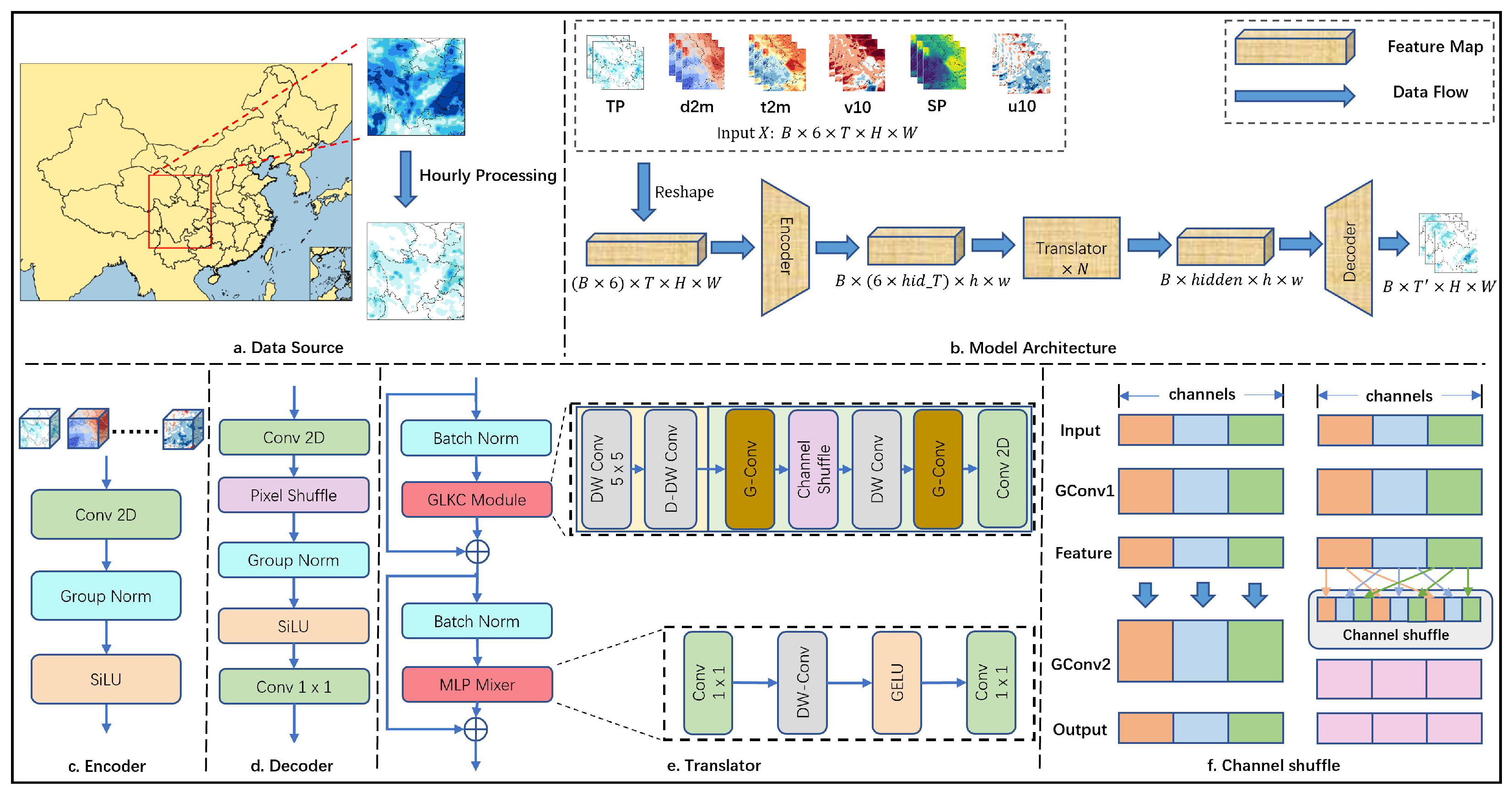
To address the deficiencies in current short-range precipitation forecasting models and further improve forecasting accuracy, we propose an advanced multi-step short-range precipitation forecasting model, GLKC-Net. The overall framework is shown in Figure 1b, which includes three parts: the encoder, spatiotemporal translator, and decoder.

Specifically, the encoder consists of a two-dimensional convolution module, with input $X\in {\mathbb{R}}^{B\times C\times T\times H\times W}$, where B, C, T, H, and W represent the batch size, number of input variables, time length, height, and width, respectively. Considering the complex spatiotemporal characteristics of meteorological data, we first merge the variable and batch dimensions to ensure the independence between different variables and obtain $X_0\in {\mathbb{R}}^{(B\times C)\times T\times H\times W}$; then, we perform spatiotemporal feature encoding for each variable in $X_0$, compressing spatial resolution while increasing the number of feature maps in time dimension, mapping them to different feature spaces, resulting in encoded output $X_{enc}\in {\mathbb{R}}^{(B\times C)\times hid\_T\times h\times w}$ which are fed into the translator to learn the spatiotemporal evolutionary relationships between data. The decoder is responsible for separating mixed spatiotemporal information from the evolved results, mapping $hid\_T$ to the target lead time length and upsampling spatial resolution back to the original size, integrating different variable in channels dimension, and finally decoding to obtain the required forecast results.

3.3. Spatial–Temporal Translator

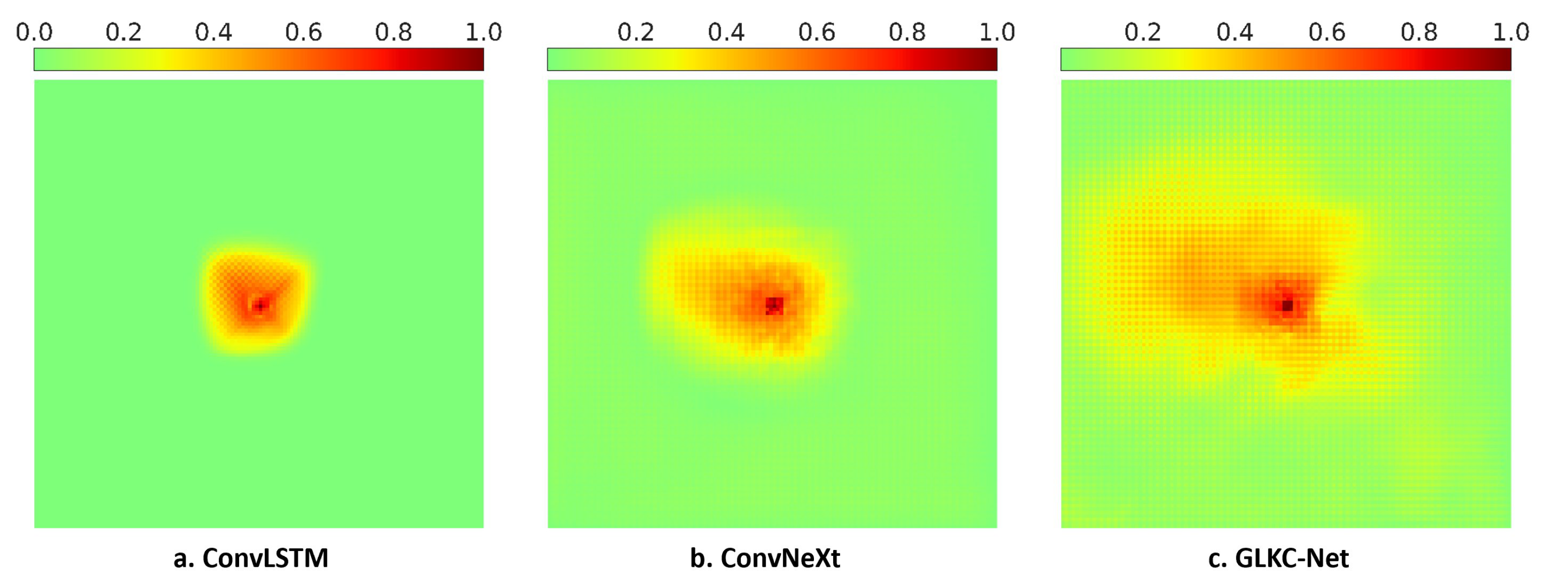
Weather systems are inherently complex and exhibit intricate spatiotemporal relationships among multiple variables across different regions. Traditional convolutional neural networks have many limitations in processing complex spatiotemporal relationships: for example, they are often constrained by relatively small effective receptive fields, as shown in Figure 2, unable to efficiently learn large-scale spatial information, and cannot model long-distance dependencies. This limitation leads to insufficient model sensitivity to changes in the global atmospheric state information from different regions, overly relying on the extraction of precipitation signals in local regions, which is not conducive to the model’s understanding of the evolution of the entire precipitation process and fails to effectively represent the spatial coherence of organized precipitation systems. Furthermore, the channel’s fully-connected approach of standard convolutions are likely to introduce unnecessary redundant information and noise, which can interfere with the model’s ability to extract key features, especially when dealing with the complex precipitation features that are coordinated by multi-variables.

Inspired by MetaFormer [49], we constructed a new spatiotemporal translator to capture complex spatiotemporal variation patterns in precipitation processes, which are primarily composed of GLKC modules and MLP−Mixer modules. The GLKC module includes a series of lightweight convolution operations that can capture long-range spatial relationships while reducing channel redundancy and strengthening the ability of the model to capture structured information. The MLP−Mixer module has a global receptive field in the channel dimension; thus, it is used for the global integration of the features obtained from the previous consecutive group module to further control channel information. This combination effectively improves the model’s understanding of spatiotemporal evolutionary relationships of meteorological variables, enhancing forecasting performance for short-range precipitation. The spatiotemporal translator can be represented by the following formula:

$$H_0=GLKC\left(Norm\left(Z\right)\right)+Z$$

(3)

$$H_1=MLP-Mixer\left(Norm\left(H_0\right)\right)+H_0$$

(4)

As shown in Figure 1e, the GLKC module contains two main components: a depth-separable large kernel convolution module and a group convolution module. Specifically, we decompose the depth-separable large kernel convolution with kernel size $K\times K$ into two lightweight convolutions: spatial long-distance convolution (depth-separable dilated convolution), with size $⌈{\displaystyle \frac{K}{d}}⌉\times ⌈{\displaystyle \frac{K}{d}}⌉$ and dilation rate d, and spatial local convolution (depth-separable convolution [50]) with size $(2d-1)\times (2d-1)$. In our experiments, K equals 21, and d equals 3, because small convolution kernels lack the necessary contextual information, while too large convolution kernels may introduce additional interfering information and lose the modeling ability for local information. The depth-separable dilated convolution enhances the spatial receptive field of the convolutional kernel by increasing the distance between each point on the convolutional kernel and filling the gaps with 0 values. However, this defect might lead to a loss of continuous information or small-scale features, which play a vital role in representing how local convection governs precipitation formation. Therefore, we added depth-separable convolution before this to fill the gap, which can ensure that while understanding the changes in the global atmospheric state, as much attention as possible is paid to the interactions of local small-scale weather systems. This can be represented as shown below:

$$LK\left(Z\right)=DW-DConv\left(DWConv\right(Z\left)\right)$$

(5)

Unlike conventional large kernel convolutions, this part only focuses on large-scale two-dimensional spatial information in each independent channel of the input feature map, with input and output channel numbers always remaining consistent, ensuring independence from time and variable information. Through this decomposition, we can obtain long-distance spatial dependency relationships with minimal parameters and computational overhead while maintaining some of the excellent characteristics originally possessed by convolutional networks.

For precipitation forecasting tasks, information interaction across different times from multi-variables is equally important. However, in traditional deep convolutional networks, using channel fully-connected approaches to learn temporal relationships for different variables would lead to most weights becoming redundant or introduce lots of noise to interfere with the learning of key patterns. Some studies [37,38,51] have shown that sparse connection methods can serve as regularization, reducing parameter sharing, redundant information, and overfitting risk while also improving generalization performance. Thus, to fully utilize position information at the same spatial locations across feature maps from different variables and reduce channel redundancy, we choose to use channel-local convolution (group convolution) for channel dimension modeling. Furthermore, we set the number of groups to match the number of selected variables. This design ensures an effective communication of information and a smooth transition between the temporal encoding performed by the encoder and the joint temporal–variable encoding within the spatiotemporal translator.

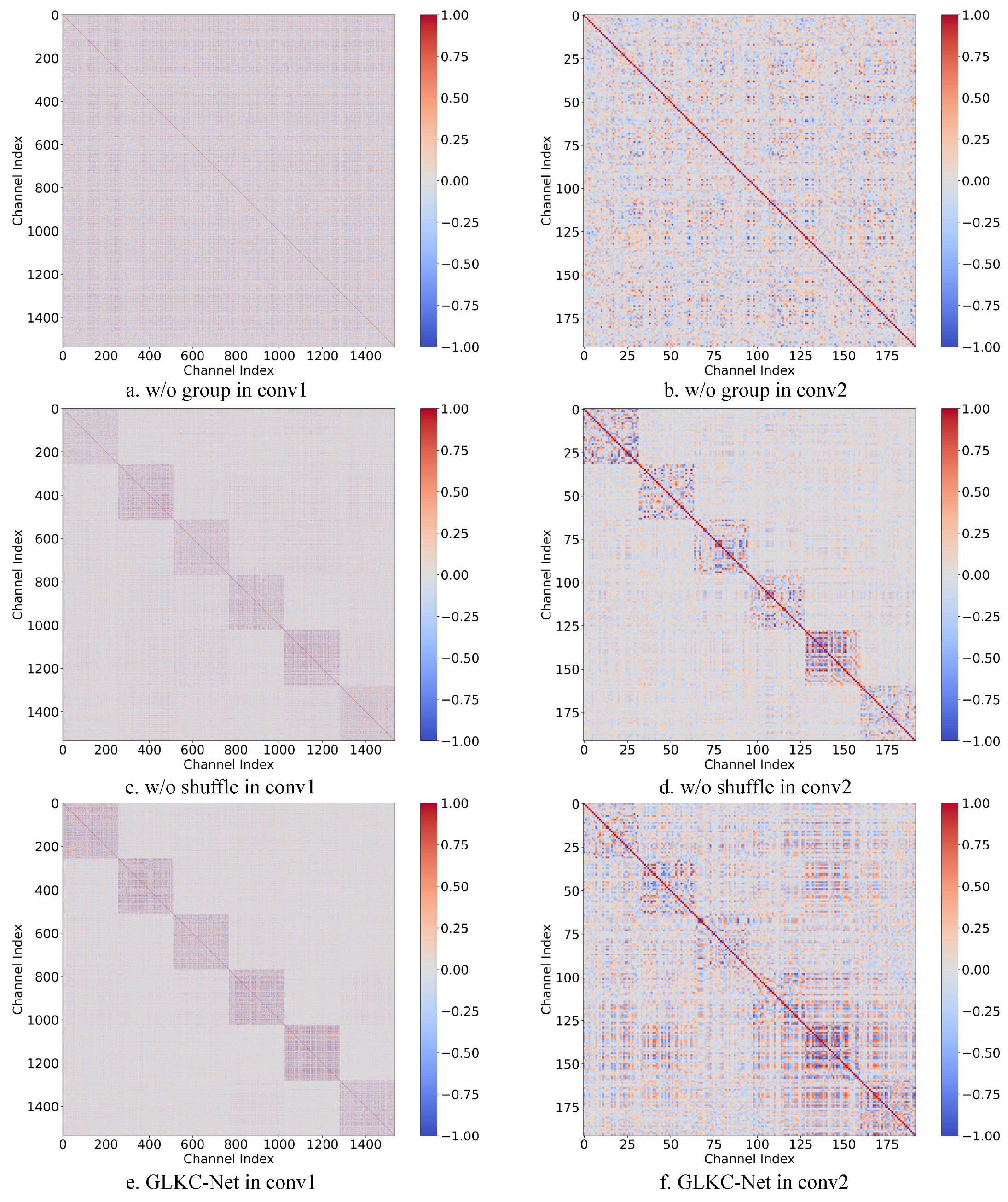
As shown in Figure 1f, we maintain the local interaction between channels in a grouped manner, weakening the correlation between feature maps in the network and making convolution kernels compute only on corresponding groups. This will be conducive to the model selectively learning more discriminative features and enhancing the channel correlations limited in the same group to reduce the introduction of redundant information and noise caused by integrating different meteorological variables at different times, as shown in Figure 3c,e. However, this is not beneficial to information interaction between features, especially in the context of various variables that have obvious correlations in atmospheric movement. Figure 1f and Figure 3d show that when stacking two group convolution together, outputs from a certain channel are only derived from a small fraction of input channels and block the information flow between channel groups, which would easily cause expression deficiencies in the model. To handle this, we introduced channel shuffle operations between two group convolutions, allowing the model to benefit more from two consecutive group convolution. First, it separates feature maps output from the previous layer’s group convolution along channels, recombines each of the feature maps from different groups to form new groupings, and then sends them to the next group convolution for computation. This enables the model to obtain a global channel sensing field of view from the previous grouping information and avoids the interference of noise or redundant information generated when directly performing full channel connection, thereby demonstrating better performance. From Figure 3, our proposed GLCK module can learn different pattern features in the first group convolution. After channel shuffle, the different features from different groups in the previous layer can be obtained through grouping, thereby extracting the global channel features. Compared with continuous ordinary convolution, it can effectively address the problem of inconsistency and improve the model’s ability to recognize complex precipitation features from multiple variables at different times.

To further enhance the representation capability of grouped features, we added an MLP-Mixer module after the GLKC module, aggregating feature information between channels through pointwise convolution. Specifically, we first expand the input feature map in the channel dimension through pointwise convolution to enrich feature content; then, we extract spatial features through depth-separable convolution and finally use pointwise convolution to fuse features from different channels and compress them back to their original size.

3.4. Multi-Thresholds Adaptive Loss Function

The Mean Squared Error (MSE) and Mean Absolute Error (MAE) are commonly used loss functions for optimizing regression problems in deep learning. From a statistical perspective, they can be viewed as the result of the maximum likelihood estimation of model parameters under the assumption that data follow Gaussian and Laplace distributions, respectively, by minimizing the negative log-likelihood function. However, this significantly differs from the “long-tail distribution” present in precipitation data. To enhance the model’s ability to handle imbalanced data, we propose MTA Loss, which is an adaptive loss function based on multiple percentile threshold divisions. This loss function efficiently measures precipitation errors at different magnitudes, adaptively weighting losses across thresholds by mining hard samples and thereby weakening the weights of simple samples, increasing the contribution of hard samples to the loss function value, strengthening the model’s focus on it, and improving forecasting performance for extreme anomalous precipitation events.

The Probability of Detection (POD), also known as recall, ranges from 0 to 1 and represents the proportion of correctly forecasted precipitation areas to actual precipitation areas at a specified threshold. Specifically, we designed a continuously differentiable adaptive weighting loss function based on multiple thresholds. We use the sigmoid function to measure the distance between predicted results and thresholds to achieve the categorical division of continuous values, expressing the loss function as an approximation of 1-POD, thereby maximizing the POD and improving the model’s hit rate. Thresholds corresponding to different data in each batch are selected according to set percentiles to adapt to the abrupt characteristics of precipitation. Finally, by using the ratio of incorrectly forecasted samples (FP and FN) to grid points exceeding the threshold in true samples at each threshold for re-weighting the loss function at corresponding thresholds, the model’s focus can be dynamically adjusted based on its forecasting performance for precipitation of different intensities. This increases attention to loss terms with higher false alarm proportions and decreases attention to those with lower false alarm proportions, effectively enhancing the forecasting capability for hard samples. This method can be represented by the following equation:

$$MTALoss=W_{0.7}·L_{0.7}^c+W_{0.95}·L_{0.95}^c+W_{0.99}·L_{0.99}^c$$

(6)

$$W_i=(F{P}_i+F{N}_i)/(T{P}_i+F{N}_i)$$

(7)

$$L_i^c={(1-\sum _k(\sigma (c\ast (I_k-i))\times \sigma (c\ast ({\hat{I}}_k-i)))/N)}^2$$

(8)

In this paper, we select 70%, 95%, and 99% as the threshold percentiles for the function on each batch. $L_i^c$ represents the magnitude of the loss function under threshold i, c equals 20 as a scaling factor, $\sigma$ is the sigmoid function, and N equals $T{P}_i+F{N}_i$. $I_k$ and $\widehat{I_k}$ represent the true value and predicted value of pixel k. When the true value exceeds the threshold to a certain extent, the scaling factor can make $\sigma (c\ast (I_k-i))$ approach 1, and conversely approach 0, similarly for $\widehat{I_k}$. Only when both $\sigma (c\ast (I_k-i))$ and $\sigma (c\ast (\widehat{I_k}-i))$ are 1 will their product be 1; in all other cases, it is 0. Thus, the numerator can be considered an approximation of TP, achieving the minimization of 1-POD through back propagation and parameter updates. This loss function can be added as a regularization term after the MSE loss to compensate for performance deficiencies caused by data distribution imbalance at specific thresholds, as shown in the following formula, where $\alpha$ is a weighting factor:

$$Loss=MSE+\alpha ·MTALoss$$

(9)

4. Experiments

4.1. Datasets Description

To evaluate the effectiveness and generalization capability of our proposed methods, we selected precipitation data from two distinct datasets, ERA5-Land and CMPAS, as prediction targets, while utilizing the extensive meteorological variables from ERA5-Land as auxiliary covariates. The details of the datasets employed are described below:

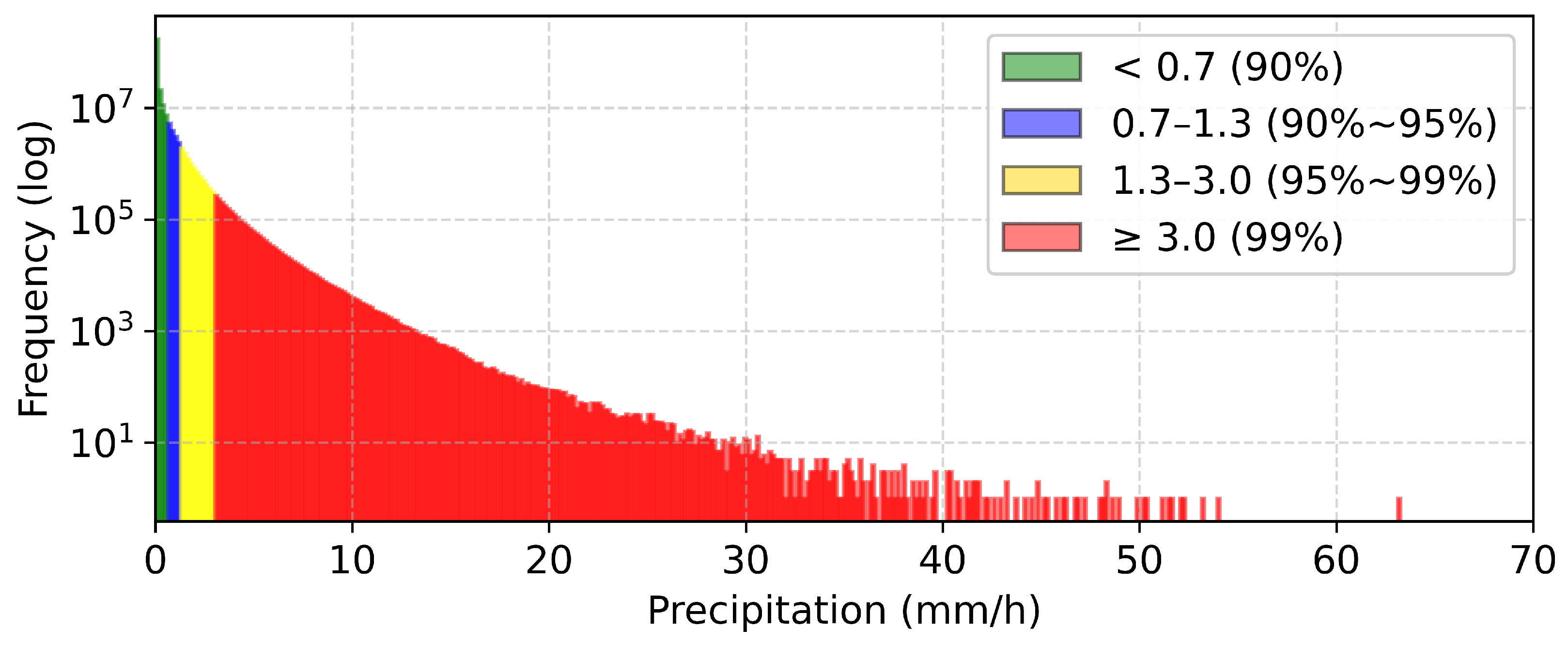
(1) ERA5-Land: ECMWF Reanalysis v5-Land (ERA5-Land) is a global reanalysis dataset developed by ECMWF based on ERA5 reanalysis data [52]. It further improves the spatial resolution of ERA5, enhances the accuracy of land surface results, and provides consistent reconstruction results for multiple meteorological variables on an hourly, 0.1° latitude–longitude grid from 1950 to the present. In this paper, we select 25.2–37.9° N, 96.4–109.1° E as the study area, as shown in Figure 1a, mainly covering southwestern China, including Sichuan, Chongqing, Guizhou, and other provinces and cities, with a spatial size of 128 × 128 after cropping. Using a sliding window approach to construct the dataset, data from May to September 2018 to 2021 were used for model training, while 2022 and 2023 for model validation and testing, respectively. The training set contains 14,688 consecutive hourly observation samples, while the validation and test sets contain 3672 samples each. One sample covers six variables: the total precipitation, u-component of wind, v-component of wind, temperature, dew point temperature, and surface pressure, which are closely related to the precipitation formation. To further illustrate the long-tail distribution characteristics of precipitation data, we visualized the distribution of precipitation intensity in the training set, as shown in Figure 4. It should be noted that the total precipitation in the original data of ERA5-Land denotes the cumulative total precipitation for the future 24 h starting from 00:00 on a given day; i.e., 01 represents cumulative precipitation between 00 and 01, 02 represents cumulative precipitation between 00 and 02, and so on. Therefore, we calculated hourly total precipitation representations by differencing adjacent time points for use in our task of forecasting hourly precipitation for the next 12 h.

$$t{p}_{\left[mm\right]}=\left\{\begin{array}{c}t{p}_h\left[m\right]·1000,h=01UTC\hfill \\ (t{p}_h\left[m\right]-t{p}_{h-1}\left[m\right])·1000,otherwise\hfill \end{array}\right.$$

(10)

(2) CMPAS: The CMPAS is an advanced multi-source analysis product developed by the China Meteorological Administration (CMA), combining satellite, radar, and gauge observations to provide comprehensive, high-resolution, and precise data for weather forecasting research. It includes four types of precipitation products: CMPAS_5km_FAST, CMPAS_5km_FRT, CMPAS_1km_RT, and CMAPS_1km_NRT. In this paper, we select CMPAS_1km_NRT, which provides near-real-time hourly precipitation observations with a 0.01° latitude–longitude grid from 2020 to 2023. To harmonize the spatial resolution, we crop CMPAS to the same area as ERA5-Land and utilize bilinear interpolation to interpolate it to the same size. Due to the varying degrees of missing and abnormal data in some time periods, we conducted preprocessing on this and split it into three parts. May to September 2020 to 2022 were used for model training, May to July 2023 were used for validation, and August to September were used for result testing.

Finally, to eliminate the differences in numerical magnitude and distribution between variables caused by dimensions, enhance model training stability and improve the convergence speed, we standardized different variables using min–max normalization:

$${\chi }^{\prime }={\displaystyle \frac{x-x_{min}}{x_{max}-x_{min}}}$$

(11)

4.2. Implementation Details

This paper uses multiple meteorological elements from the ERA5-Land and the CMPAS datasets to make a precipitation forecast for 12 h. All experiments were conducted based on the Linux operating system and the PyTorch-2.5.1 deep learning framework. During model training, Adaptive Moment Estimation (Adam) was selected as the optimizer, with an initial learning rate set at 0.0001 and a linear decay strategy adopted to adjust it based on changes in validation set loss during training, with a decay rate of 0.5. The batch size was set to 12, the maximum number of training epochs was set to 200, and an early stopping strategy was used to obtain a model with stable performance.

4.3. Evaluating Metrics

To evaluate the performance of our method, in addition to MSE and PCC (Pearson Correlation Coefficient), this paper also selected various classification-based skill scores commonly used in precipitation forecasting, including the Critical Success Index (CSI), Heidke Skill Score (HSS), Probability of Detection (POD), and False Alarm Rate (FAR), to conduct more comprehensive and integrated quantitative assessments of the model’s forecasting results from different perspectives. For classification metrics, three different levels of precipitation intensity—0.1 mm/h, 1.0 mm/h, and 2.5 mm/h—were selected as thresholds for category division. As shown in

Table 1. Confusion matrix.

	Prediction = 1	Prediction = 0
Observation = 1	TP	FN
Observation = 0	FP	TN

, for classification skill scores under a certain threshold, pixel values of forecasted and true results are first compared with the corresponding threshold with values greater or less than the threshold converted to 1 or 0. Subsequently, TP, FN, FP, and TN are calculated in sequence. These performance evaluation metrics can be defined as shown below:

$$CSI={\displaystyle \frac{TP}{TP+FP+FN}}$$

(12)

$$POD={\displaystyle \frac{TP}{TP+FN}}$$

(13)

$$FAR={\displaystyle \frac{FP}{TP+FP}}$$

(14)

$$HSS={\displaystyle \frac{2\times (TP\times TN-FP\times FN)}{(TP+FN)(TN+FN)+(TP+FP)(FP+TN)}}$$

(15)

$$MSE={\displaystyle \frac{1}{N}}\sum _{i=1}^N{(y_{pred}^i-y_{obs}^i)}^2$$

(16)

$$PCC={\displaystyle \frac{{\sum }_{i=1}^N(y_{pred}^i-{\overline{Y}}_{pred})(y_{obs}^i-{\overline{Y}}_{obs})}{\sqrt{{\sum }_{i=1}^N{(y_{pred}^i-{\overline{Y}}_{pred})}^2}\sqrt{{\sum }_{i=1}^N{(y_{obs}^i-{\overline{Y}}_{obs})}^2}}}$$

(17)

4.4. Comparative Experiments

To validate the effectiveness of our proposed method, we selected eight models that have demonstrated outstanding performance in precipitation forecasting and spatiotemporal sequence prediction tasks as baseline models for comprehensive evaluation on the test set. Due to the inequality of training resources and the limitations of open-source code, this paper does not compare them with the large models mentioned in the introduction. These baseline models in this paper can be classified into three types of models: the ConvLSTM [19] and TrajGRU [20] models based on the RNN framework, the SimVP [34], ConvNeXt [53], and MogaNet [54] models based on the CNN framework, and the RainFormer [55], RainHCNet [56], and STAA [1] models based on the Transformer framework.

Table 2. ERA5-Land: Comparison of performance indicators of each model on ERA5-Land datasets (↑ means the higher the better and ↓ means the lower the better, Bold indicates the best results, underlined values are the suboptimal ones, and ‘Rank’ is the average rank of the model on each metric).

Models	CSI ↑			POD ↑			FAR ↓			HSS ↑			MSE ↓	PCC ↑	Rank ↓
	0.1	1.0	2.5	0.1	1.0	2.5	0.1	1.0	2.5	0.1	1.0	2.5
ConvLSTM	0.4949	0.2057	0.0897	0.8196	0.2684	0.1103	0.4495	0.4685	0.2832	0.4431	0.2802	0.1297	0.2347	0.5463	7.07
TrajGRU	0.4913	0.2108	0.0893	0.8194	0.2754	0.1110	0.4557	0.4382	0.2605	0.4407	0.2863	0.1293	0.2301	0.5557	6.07
SimVP	0.4609	0.2152	0.0869	0.9006	0.2893	0.1070	0.5174	0.4579	0.2660	0.3633	0.2914	0.1252	0.2300	0.5594	6.00
ConvNeXt	0.4453	0.2252	0.0957	0.9094	0.3023	0.1190	0.5371	0.4620	0.2700	0.3333	0.3047	0.1379	0.2258	0.5668	4.07
MogaNet	0.5075	0.2218	0.0988	0.8265	0.2956	0.1247	0.4359	0.4630	0.3132	0.4644	0.3016	0.1431	0.2283	0.5693	3.64
RainFormer	0.4407	0.2186	0.0928	0.8959	0.3108	0.1175	0.5352	0.5441	0.3535	0.3265	0.2969	0.1351	0.2415	0.5398	6.21
RainHCNet	0.5170	0.2115	0.0899	0.7685	0.2764	0.1093	0.3943	0.4573	0.2738	0.4957	0.2883	0.1306	0.2314	0.5595	5.07
STAA	0.5055	0.2106	0.0928	0.7850	0.2754	0.1148	0.4171	0.4466	0.2471	0.4704	0.2868	0.1337	0.2272	0.5630	4.57
GLKC-Net (Ours)	0.5092	0.2334	0.1062	0.8365	0.3114	0.1353	0.4396	0.4543	0.3036	0.4625	0.3151	0.1529	0.2219	0.5792	2.29

and

Table 3. CMPAS: Comparison of performance indicators of each model on CMPAS datasets (↑ means the higher the better and ↓ means the lower the better, Bold indicates the best results, underlined values are the suboptimal ones, and ‘Rank’ is the average rank of the model on each metric).

Models	CSI ↑			POD ↑			FAR ↓			HSS ↑			MSE ↓	PCC ↑	Rank ↓
	0.1	1.0	2.5	0.1	1.0	2.5	0.1	1.0	2.5	0.1	1.0	2.5
ConvLSTM	0.2102	0.1063	0.0460	0.8175	0.1580	0.0620	0.7799	0.5633	0.2492	0.1752	0.1497	0.0693	0.7365	0.2490	5.05
TrajGRU	0.2097	0.1027	0.0440	0.7529	0.1494	0.0579	0.7758	0.5239	0.1822	0.1794	0.1446	0.0656	0.7315	0.2546	6.14
SimVP	0.2235	0.1091	0.0446	0.7614	0.1544	0.0586	0.7620	0.4312	0.1681	0.2084	0.1540	0.0669	0.7254	0.2729	3.93
ConvNeXt	0.2385	0.1081	0.0446	0.7216	0.1502	0.0572	0.7408	0.4553	0.1696	0.2343	0.1534	0.0672	0.7211	0.2794	3.93
MogaNet	0.1646	0.1176	0.0456	0.9038	0.1663	0.0586	0.8320	0.5771	0.2655	0.0875	0.1666	0.0694	0.7367	0.2654	5.21
RainFormer	0.2007	0.0992	0.0380	0.6137	0.1287	0.0462	0.7616	0.5527	0.3548	0.1824	0.1426	0.0589	0.7529	0.2324	8.07
RainHCNet	0.2412	0.0975	0.0404	0.6456	0.1286	0.0500	0.6900	0.4255	0.1929	0.2436	0.1380	0.0612	0.7357	0.2641	5.79
STAA	0.2276	0.1125	0.0423	0.7868	0.1587	0.0546	0.7588	0.4680	0.1806	0.2105	0.1593	0.0639	0.7273	0.2730	4.21
GLKC-Net (Ours)	0.2467	0.1235	0.0511	0.7589	0.1769	0.0674	0.7352	0.5275	0.2325	0.2428	0.1743	0.0769	0.7216	0.2798	2.21

present the average performance of each model across different evaluation metrics for 12 h precipitation forecasting on ERA5-Land and CMPAS, respectively.

As shown in Table 2, our model demonstrates superior performance in MSE and PCC compared to the baseline models, indicating better consistency between forecasted results and ground truth values across the global range. Regarding threshold-based binary classification skill scores, our model maintains excellent performance, achieving the best results on CSI, POD, and HSS for higher precipitation intensities with improvements of 7.49%, 8.5%, and 6.85%, respectively, at the 2.5 mm/h precipitation threshold compared to the second-best model. However, for the POD at the 0.1 mm/h precipitation threshold, the GLKC-Net shows a noticeable gap compared to the SimVP, ConvNeXt, and RainFormer, decreasing by 7.12%, 8.02%, and 6.63%. This primarily occurs because these models have the problem of “more light rain and less heavy rain”, which tends to inflate forecast values to achieve higher hit rates, substantially increasing false alarm risks, with the FAR increasing by 17.70%, 22.18%, and 21.75%. This ultimately leads to significant performance degradation in comprehensive metrics that combine hits, misses, and false alarms, such as HSS (decreased by 21.45%, 27.94%, and 29.41%) and CSI (decreased by 9.49%, 12.55%, and 13.45%), indicating lower actual forecasting skill. Overall, in comparison with the baseline models, our model achieved the best average rank among all metrics, demonstrating more comprehensive and superior forecasting capabilities, particularly for relatively higher-intensity precipitation events. Similar to the results on the ERA5-Land dataset, our model also achieved the best average rank on the CMPAS dataset compared with baseline models, as shown in Table 3. The proposed model GLKC-Net shows an excellent advantage on CSI, POD, and HSS, except for POD at 0.1 mm/h, with improvements of 5.02%, 6.37%, and 4.62% at 1.0 mm/h, and 11.09%, 8.71%, and 10.81% at 2.5 mm/h.

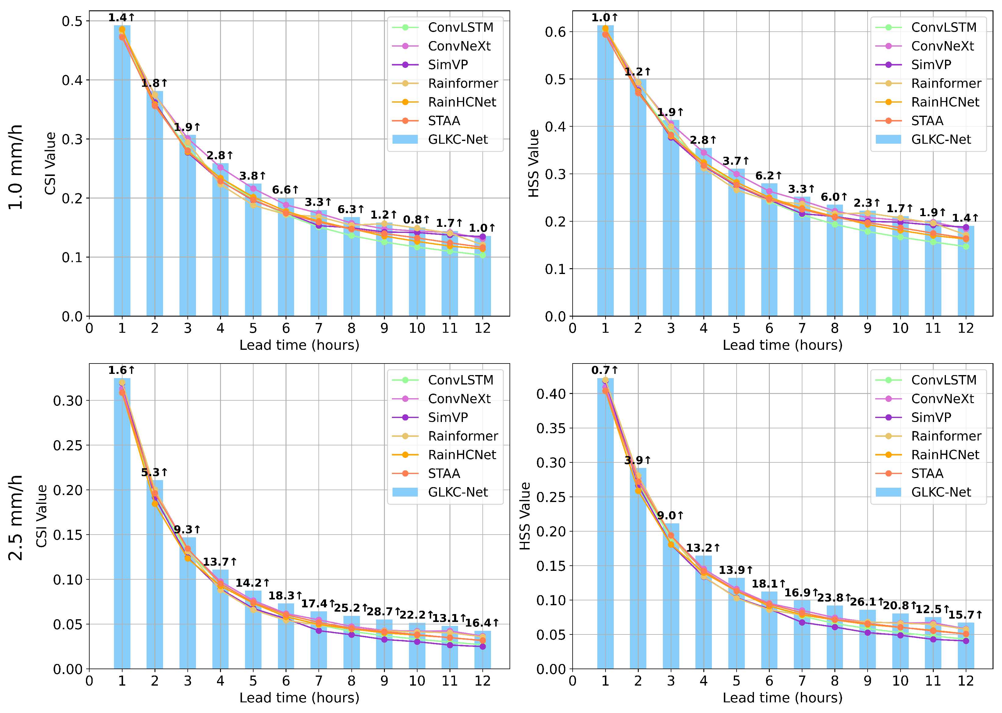
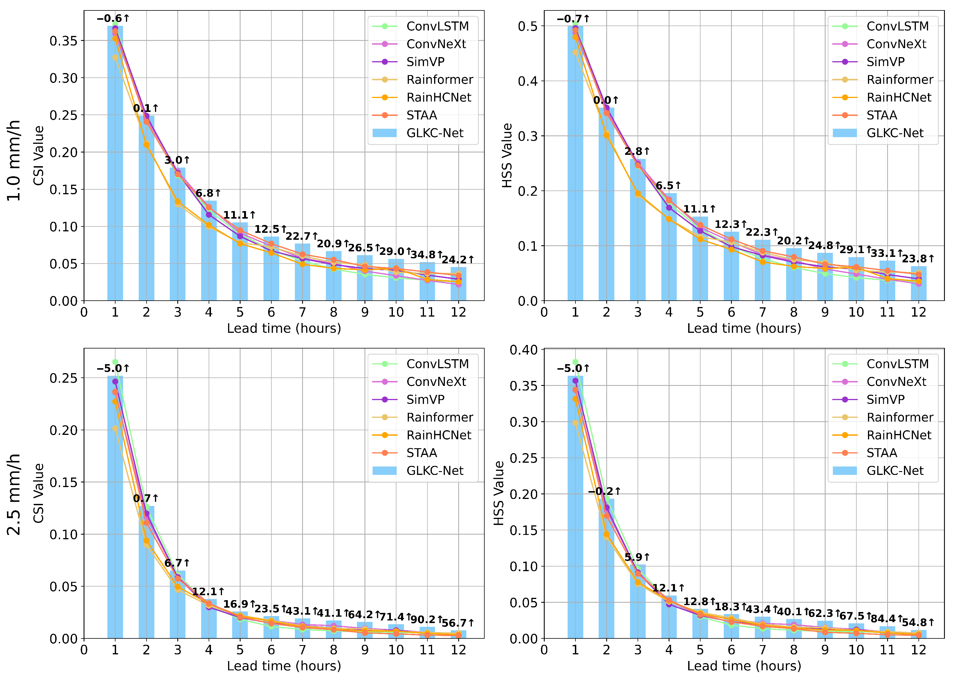
Additionally, we selected six representative models based on various frameworks to calculate CSI and ETS at different time points corresponding to precipitation intensities of 1.0 mm/h and 2.5 mm/h to investigate how systematic errors from varying forecast lead times affect different models’ forecasting capabilities under different thresholds and compare these with the proposed GLKC-Net model on ERA5-Land and CMPAS datasets, as shown in Figure 5 and Figure 6. From these figures, we can observe that as time progresses, the CSI and HSS for all models have rapidly decreased, especially for metrics at 2.5 mm/h and the CMPAS dataset, and the rate of decline gradually slows. These indicate that with the extension of lead time, the model forecasting skill has a significant decrease, and this change has a greater impact on the precipitation intensity of higher thresholds, which could be due to the fact that all models, which are affected by precipitation data distribution, exhibit deficiencies in forecasting stronger precipitation events and are more sensitive to lead times.

For the process shown in Figure 5, the GLKC-Net model consistently maintains a relatively higher level of forecasting skill. This suggests that while the forecasting capabilities of all models weaken with extended lead times, our model demonstrates better stability in this regard, achieving good accuracy at all time points. Specifically, in the initial stages, performance differences among models are not particularly pronounced. After three hours, the lines begin to diverge with skill scores showing more significant disparities. Meanwhile, the improvements of our model were also constantly growing until they began to decline in the last two hours. At 1.0 mm/h, the CNN-based models gradually stabilize in performance around the seventh hour, while the RNN-based recurrent models continue to decline, highlighting the limitations of autoregressive modeling approaches, which lead to more severe error accumulation in long-range forecasting, and the transformer-based model is somewhere in between. At 2.5 mm/h, the transformer-based models perform better than SimVP and ConvLSTM, and they have comparable skill with ConvNeXt. Overall, our model maintains superior forecasting performance from the initial to final stages with particularly notable advantages between 3 and 10 h. For the CMPAS dataset, shown in Figure 6, the proposed model GLKC-Net seems to perform worse than ConvLSTM at the first hour. However, after the second hour, the advantages of our model are gradually becoming obvious, the performance of baseline models deteriorates more quickly, and there is a very significant gap compared with the transformer-based models. Therefore, on the whole, our model can still achieve a higher forecasting skill compared to baseline models.

4.5. Case Study

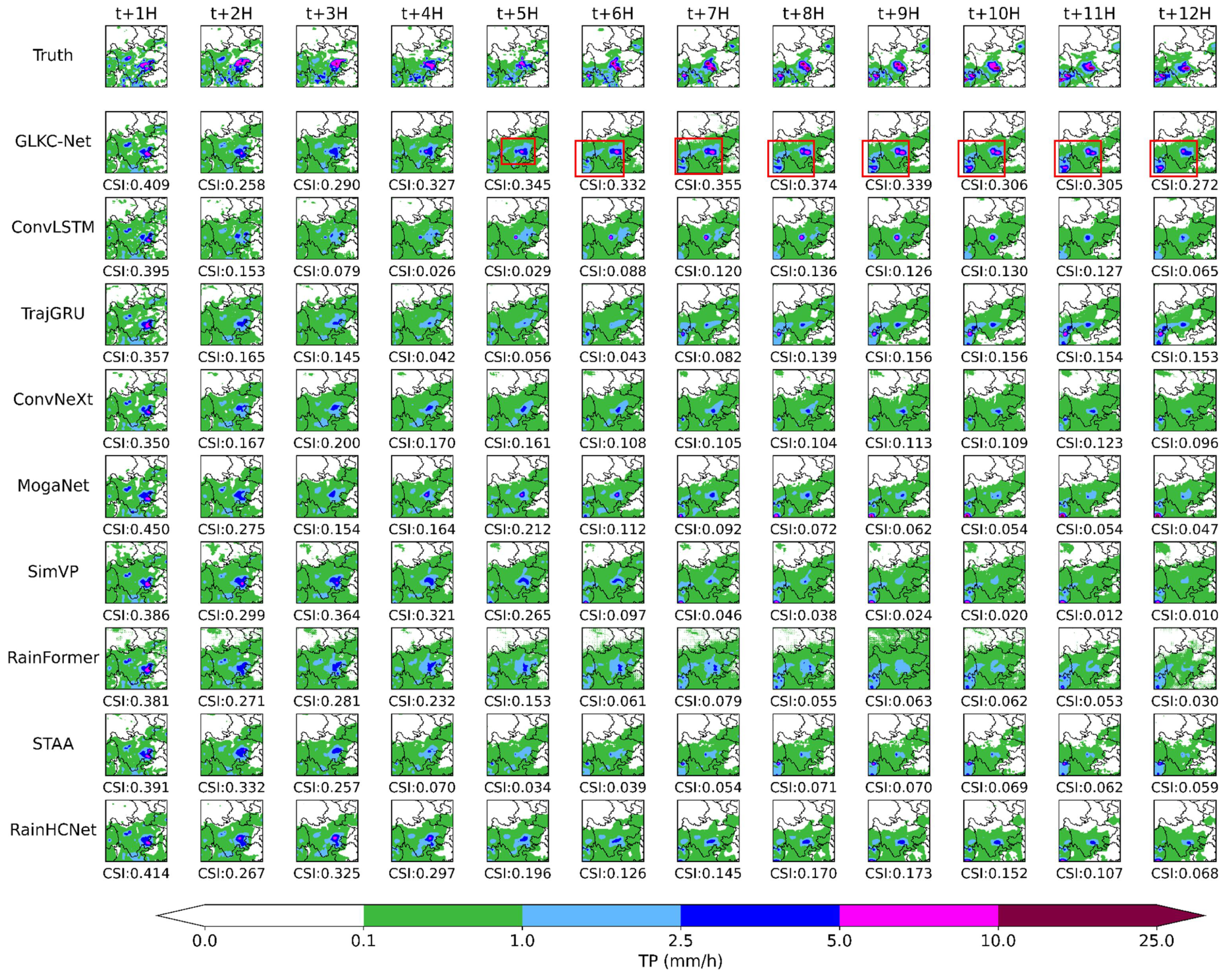
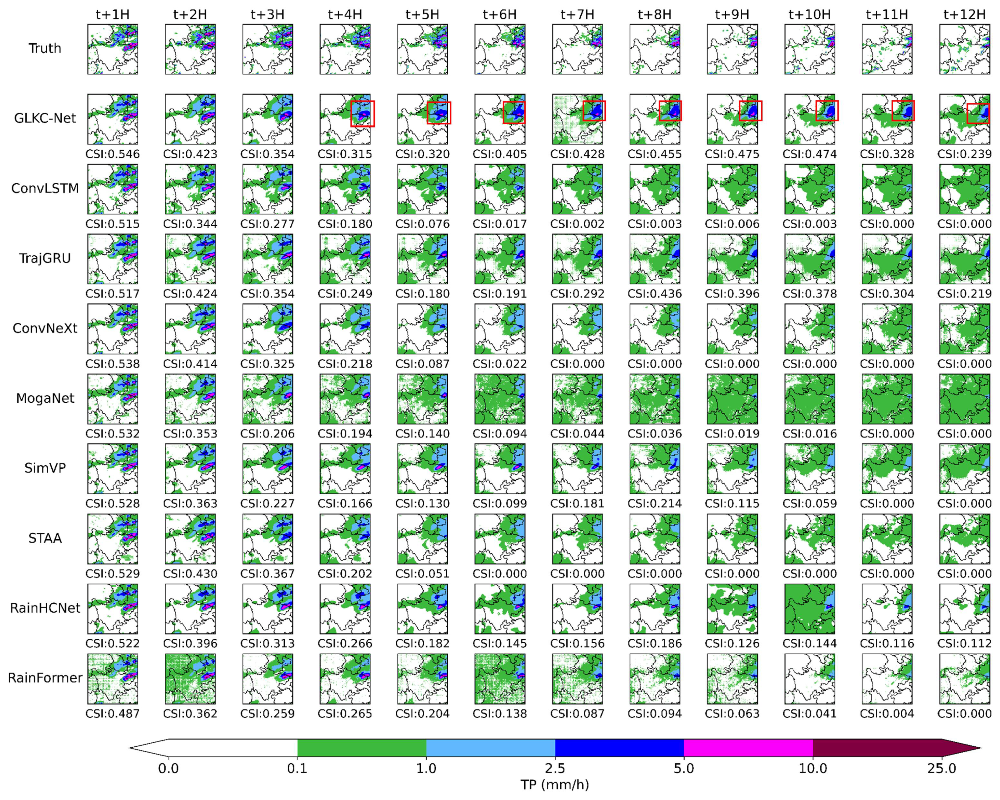
As shown in Figure 7, we use a development process of strong precipitation in the study area from 13:00 UTC on 11 August 2023 to 00:00 UTC on 12 August 2023 as an example, where the maximum precipitation reached 26.94 mm/h. We further analyze the performance of different models, annotating CSI values at the 2.5 mm/h precipitation intensity threshold to quantify the models’ forecasting capabilities for relatively strong precipitation events. In the first hour of forecasting, a strong precipitation center appeared in southeastern Sichuan, and all models were able to simulate its main characteristics well. However, as the forecast lead time increased, forecasting performance rapidly declined. Between 2 and 5 h, the precipitation characteristics continuously changed, generally moving toward central Sichuan with a weakening trend. During this period, the ConvLSTM and TrajGRU failed to identify changes in the intensity and position of precipitation centers spatially. Meanwhile, ConvNeXt and MogaNet, although able to identify precipitation with greater intensity, were too conservative in estimating precipitation coverage, resulting in low CSI skill scores. At the 6 h time point, the precipitation characteristics in the region underwent dramatic changes, with two areas exceeding 10 mm/h suddenly appearing in central and southeastern Sichuan, posing significant challenges for model forecast. Nevertheless, our model maintained good forecasting performance, capturing the main features of the overall distribution. From 7 to 12 h, our model continued to maintain effective predictions for the two main precipitation areas, especially for local precipitation events with intensities greater than 5 mm/h. While ConvLSTM and TrajGRU could also predict the existence of strong precipitation features, they showed significant deviations in predicting precipitation locations. The CNN-based models like ConvNeXt completely lost or deviated from the true distribution characteristics. Throughout the entire process, as time increased, our model showed some overestimation in Guizhou and the northwestern Sichuan, but it captured the main strong precipitation features and change processes well, demonstrating significant advantages compared to the baseline models. Similar to Figure 7, we select a process of the gradual dissipation of heavy precipitation in CMPAS from 22:00 UTC on 18 September to 09:00 UTC on 19 September 2023, as shown in Figure 8. For the first two hours, two precipitation centers appeared in Shaanxi Province and at the junction of Shaanxi Province and Sichuan Province. The proposed model GLKC-Net had comparable prediction performance with TrajGRU, ConvNeXt, and STAA, and it can predict the shape and location of precipitation distribution accurately. From three to seven hours, the two precipitation centers start to approach each other. All the models failed to accurately capture this gradual change and estimated the fusion of the precipitation center too early at three or four hours, and the forecasting results of the model have now declined to varying degrees. Among them, the performances of ConvLSTM, ConvNeXt, and STAA have declined most significantly, losing the prediction of precipitation centers and resulting in a relatively low precision. In addition, the remaining models have certain predictive capabilities for this process, but our model has demonstrated the most accurate results. Over the last five hours, the center of precipitation began to move eastward and gradually disappeared in the study area. Only GLKC-Net, RainHCNet, and TrajGRU can predict the distribution of precipitation greater than 2.5 mm/h, and GLKC-Net achieved the highest CSI value, which covered a large area of precipitation, greatly reducing the number of false negatives.

4.6. Results for MTA Loss

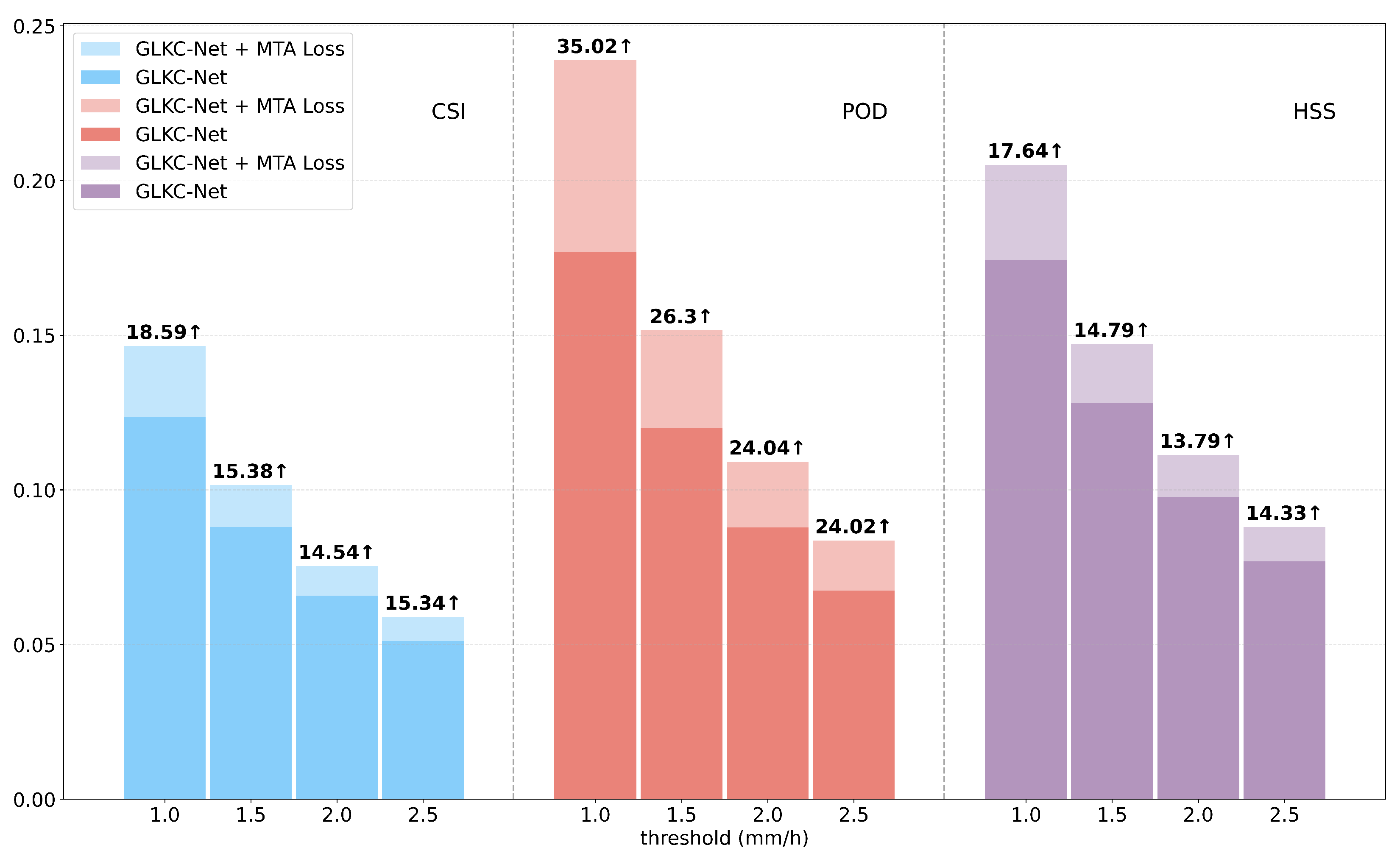
To evaluate the ability of MTA Loss for alleviating the significant decline in the accuracy of extreme precipitation forecasts caused by imbalanced data distribution, we conducted a comprehensive experiment on both ERA5-Land and CMPAS datasets. Firstly, we compare it with several loss functions, which are dealing with imbalanced data distributions, including Multisigmoid Loss [48], Focal-R [41], B-Huber [23], and B-MSE [20], to show the advantages of our method. And then, by visualizing the error map and comparing the CSI and HSS values for four thresholds from 1.0 mm/h to 2.5 mm/h, we show the improvements of the model’s predictive ability for extreme precipitation events before and after using the loss function.

As shown in

Table 4. Comparison of different performance indicators of different loss function on ERA5-Land (↑ means the higher the better and ↓ means the lower the better, Bold indicates the best results, underlined values are the suboptimal ones).

Methods	CSI ↑		POD ↑		HSS ↑		MSE ↓
	1.0	2.5	1.0	2.5	1.0	2.5
MSE	0.2334	0.1062	0.3114	0.1353	0.3151	0.1529	0.2219
Multisigmoid Loss	0.2279	0.1009	0.2957	0.1252	0.3102	0.1461	0.2258
Focal-R	0.2174	0.0957	0.2751	0.1154	0.2965	0.1384	0.2208
B-Huber	0.2082	0.0838	0.2578	0.0973	0.2843	0.1201	0.2224
B-MSE	0.2359	0.1397	0.6304	0.4070	0.3039	0.2054	0.5669
MTA Loss (Ours)	0.2384	0.1173	0.3307	0.1575	0.3209	0.1694	0.2301

and

Table 5. Comparison of different performance indicators of different loss function on CMPAS (↑ means the higher the better and ↓ means the lower the better, Bold indicates the best results, underlined values are the suboptimal ones).

Methods	CSI ↑		POD ↑		HSS ↑		MSE ↓
	1.0	2.5	1.0	2.5	1.0	2.5
MSE	0.1235	0.0511	0.1769	0.0674	0.1743	0.0769	0.7216
Multisigmoid Loss	0.0640	0.0327	0.0761	0.0398	0.0920	0.0490	0.7768
Focal-R	0.1069	0.0383	0.1401	0.0462	0.1521	0.0579	0.7234
B-Huber	0.0844	0.0293	0.1015	0.0334	0.1210	0.0443	0.7381
B-MSE	0.1105	0.0772	0.7049	0.4819	0.1314	0.1125	2.7943
MTA Loss (Ours)	0.1465	0.0589	0.2389	0.0836	0.2051	0.0880	0.7245

, the MTA Loss we proposed outperforms other loss functions in most metrics, especially for the Multisigmoid Loss, Focal-R, and B-Huber. Although they are relatively better in terms of MSE, this is mainly due to the underestimation of intense precipitation events, resulting in significant declines in CSI, POD, and HSS. Compared to B-MSE, our method exhibits a noticeable gap in POD as well as in CSI and HSS at the precipitation intensity threshold of 2.5 mm/h. However, it does not outperform our approach in terms of CSI and HSS at the 1.0 mm/h threshold, especially on the CMPAS dataset. This discrepancy may stem from the fixed large weights assigned to high-threshold precipitation events in B-MSE, which likely leads to an overforecasting of precipitation magnitudes and consequently results in a substantial degradation of the MSE metric. In fact, the MSE quantitatively measures the overall error between forecasted and observed precipitation. A larger MSE usually indicates that the model has significant numerical errors and also suggests that there may be a large magnitude difference. Combining the results of classification metrics, it becomes evident that although B-MSE achieves a high POD for low-threshold precipitation, its CSI and HSS degrade relative to the baseline model, indicating no genuine enhancement in forecasting skill. Consequently, the apparent improvement at high thresholds comes at the expense of predictive accuracy for routine precipitation events. In operational contexts, this trade-off may manifest as an overestimation of precipitation coverage area, resulting in a large number of false alarms in areas without precipitation and deviations in the intensity of areas with precipitation. This can cause significant misguidance in task scheduling and resource allocation in practical applications. Overall, our method can significantly improve the performance of the model in classification metrics while sacrificing very little in terms of MSE. It can maintain the balance between regression and classification accuracy. Therefore, MTA Loss is more practical and effective compared to other loss functions.

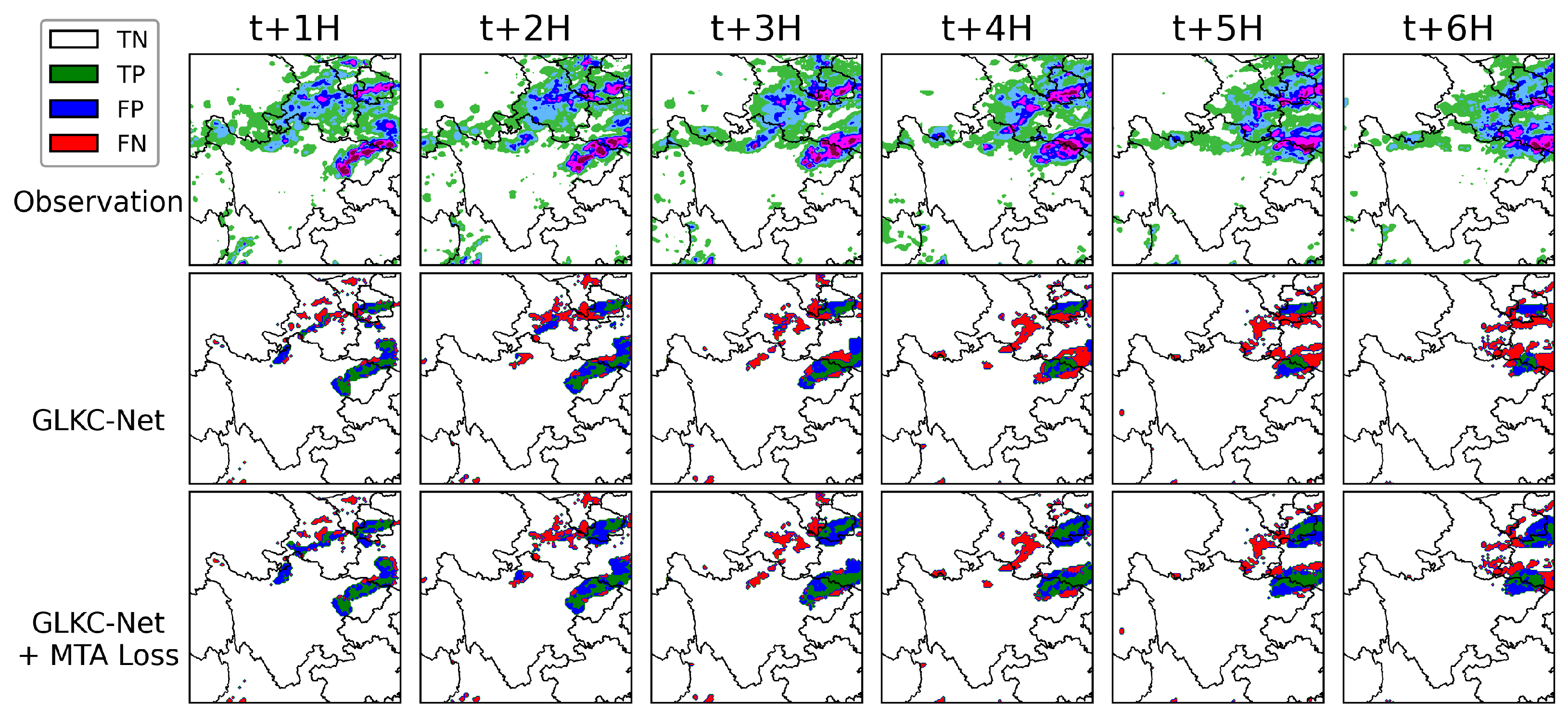
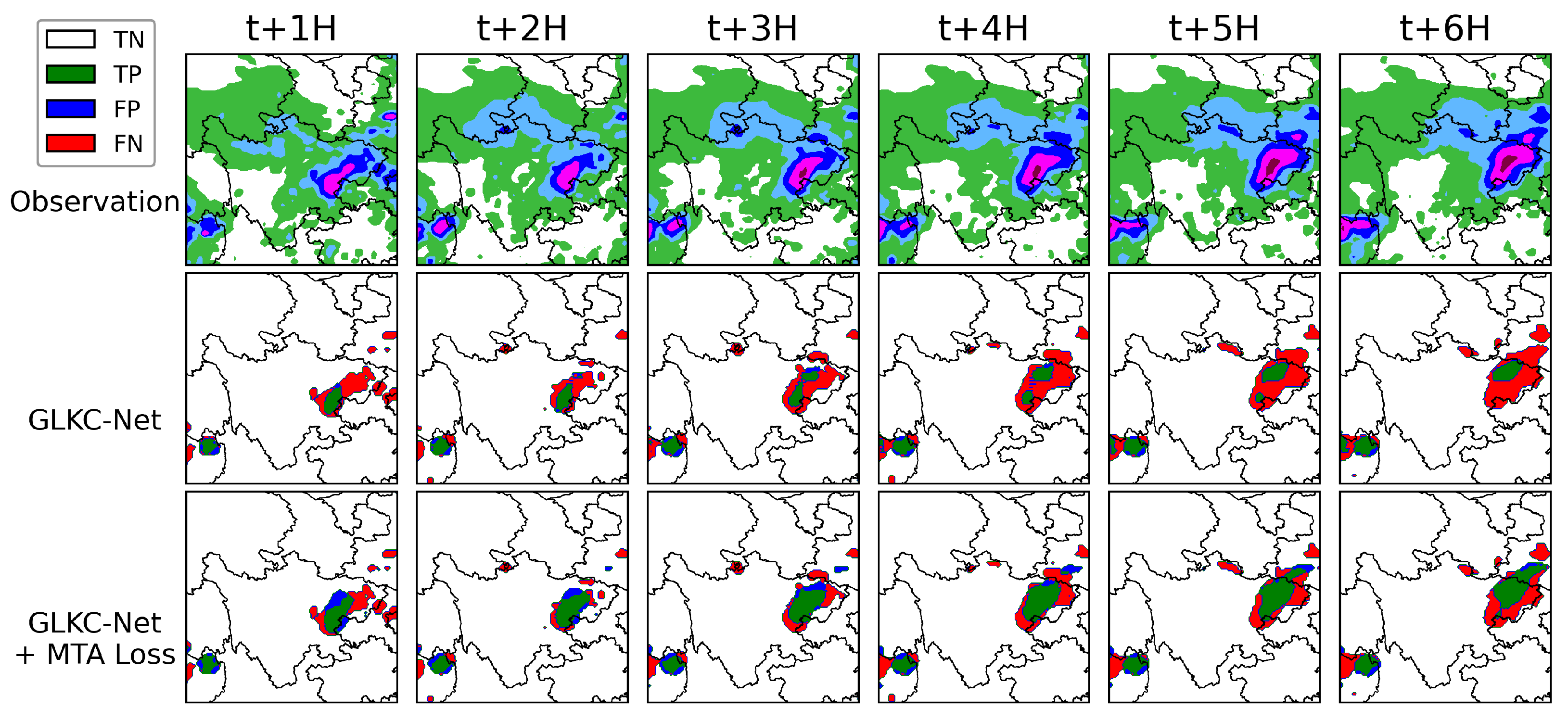
In Figure 9 and Figure 10, we visualize the hits (green), missed alarms (red), and false alarms (blue) under a precipitation intensity of 2.5 mm/h. Although the original model has a certain predictive ability for this heavy precipitation process, there are still large areas of missed forecasts. In contrast, the model, after adding the loss function, can make up for this defect and greatly improve the hit rate of the model.

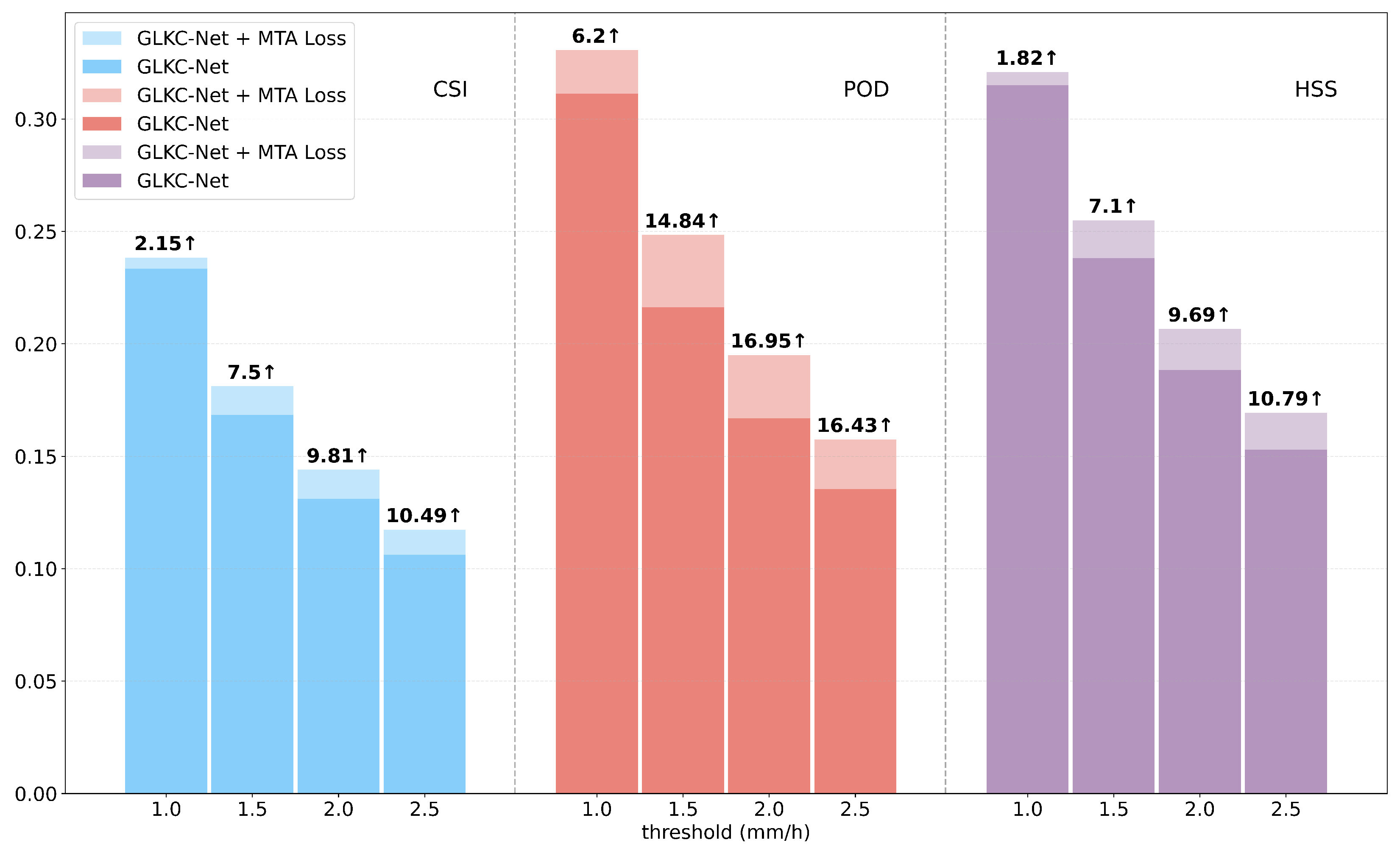
As clearly shown in Figure 11, we demonstrate the improvement in forecasting capability for heavy precipitation after adding the loss function to the original model on the ERA5-Land dataset. With the increase in precipitation intensity, the performance improvement brought by MTA Loss to the model becomes more obvious, and at the threshold of 2.5 mm/h, CSI, POD, and HSS reach 10.49%, 16.43%, and 10.79%, respectively. For the results on the CMPAS dataset, in Figure 12, we can draw a similar conclusion. Among them, the improvement of POD was the most significant, reaching an average of 27.35% at different thresholds. CSI and HSS also increased by an average of 15.96% and 15.14%, respectively. These indicate that our proposed MTA Loss automatically adjusts focus on hard samples, can address forecast biases from data imbalance problems in precipitation tasks, and strengthens forecasting skills for extreme precipitation.

4.7. Ablation Studies

To analyze the impacts of different model components on learning precipitation features for forecasting results, we conducted ablation experiments by comparing different model configurations on the two test datasets. Specifically, we take the MLP module with only the inverted bottleneck structure as the baseline model (first row in

Table 6. ERA5-Land: ablation studies results (↑ means the higher the better, Bold indicates the best results).

LK	Group	Channel Shuffle	CSI ↑		POD ↑		HSS ↑
			1.0	2.5	1.0	2.5	1.0	2.5
–	–	–	0.2108	0.0963	0.2741	0.1191	0.2867	0.1376
–	✓	–	0.2236	0.0987	0.2926	0.1217	0.3030	0.1419
✓	–	–	0.2089	0.0950	0.2638	0.1156	0.2848	0.1367
–	✓	✓	0.2248	0.1023	0.2967	0.1291	0.3039	0.1465
✓	–	✓	0.2249	0.0985	0.2960	0.1215	0.3051	0.1420
✓	✓	–	0.2278	0.0984	0.2992	0.1203	0.3084	0.1426
✓	✓	✓	0.2334	0.1062	0.3114	0.1353	0.3151	0.1529

and

Table 7. CMPAS: ablation studies results (↑ means the higher the better, Bold indicates the best results).

LK	Group	Channel Shuffle	CSI ↑		POD ↑		HSS ↑
			1.0	2.5	1.0	2.5	1.0	2.5
–	–	–	0.1113	0.0444	0.1578	0.0574	0.1577	0.0669
–	✓	–	0.1181	0.0482	0.1707	0.0630	0.1667	0.0727
✓	–	–	0.1135	0.0418	0.1594	0.0532	0.1611	0.0631
–	✓	✓	0.1122	0.0469	0.1571	0.0612	0.1587	0.0702
✓	–	✓	0.1161	0.0436	0.1628	0.0559	0.1639	0.0655
✓	✓	–	0.1211	0.0480	0.1767	0.0625	0.1704	0.0722
✓	✓	✓	0.1235	0.0511	0.1769	0.0674	0.1743	0.0769

). By sequentially incorporating the large kernel convolution, group convolution, and channel shuffle methods, we construct GLKC-Net. With results shown in Table 6 and Table 7, the full model (last row, with all three components) achieves the best performance in CSI, POD, and HSS scores. Conversely, ablating any of these components from the full model leads to performance degradation, as demonstrated in the table. The reason is that without the large-kernel convolution module, the receptive field of the model will be limited by the small convolutional kernels and thus be unfavorable for understanding the characteristics of the large-scale pattern change process of different variables during precipitation. Deleting group convolution and channel shuffle operations will also lead to the model being affected by redundant information and noise generated during continuous stacking and thus hinder the information exchange, making it fail to learn useful features from complex spatiotemporal patterns among multi-variables. For example, at the threshold of 2.5 mm/h for the w/o group in Table 7, the CSI, POD, and HSS decreased by 1.80%, 2.61% and 2.09% compared with the baseline. The ablation study suggests that these various convolution modules in our proposed GLCK module have a better collaborative ability that can improve the overall performance on the two datasets and gain 11.97%, 14.18%, and 11.63% improvements for the CSI, POD, and HSS, respectively, on average, compared with the baseline.

5. Conclusions

In this paper, we proposed a deep learning model called GLKC-Net, which utilizes the multi-variables of meteorological data for multi-step short-range precipitation forecasting. Based on an encoder–translator–decoder network architecture, this model combines large kernel convolution with channel-local convolution to construct the GLCK module, achieving an efficient extraction of wide-range spatial information, alleviating the redundancy problem caused by channel fully-connected structures in traditional convolutional networks, and accurately extracting complex spatiotemporal precipitation features. Compared with some currently popular deep learning methods, it improves the overall forecasting skills across various precipitation scenarios. Additionally, we designed a new multi-threshold adaptive loss function to address the imbalanced distribution of precipitation data, enhancing the model’s forecasting capability for less frequent, difficult-to-forecast heavy precipitation events specially over southwestern China, where the traditional models often failed. The forecast experiments have clearly validated our new model’s superior ability in improving prediction skills over there. Future work will focus on how to effectively integrate multi-source data such as satellite imagery, radar, and even numerical weather prediction results, optimize network structures to improve forecasting accuracy, and enhance model interpretability to deal with the increasing challenges brought about by climate change.

References

1. Chen, M.; Yang, H.; Li, S.; Qin, X. STAA: Spatio-Temporal Alignment Attention for Short-Term Precipitation Forecasting. IEEE Geosci. Remote Sens. Lett. 2024, 21, 1003105. [Google Scholar] [CrossRef] [Scilit]
2. Fang, W.; Shen, L.; Sheng, V.S. VRNet: A Vivid Radar Network for Precipitation Nowcasting. IEEE Trans. Geosci. Remote Sens. 2024, 62, 4103811. [Google Scholar] [CrossRef] [Scilit]
3. Choi, H.; Choi, J.; Hwang, J.; Lee, K.; Lee, D.; Park, N. Climate modeling with neural advection–diffusion equation. Knowl. Inf. Syst. 2023, 65, 2403–2427. [Google Scholar] [CrossRef] [Scilit]
4. Huang, R.; Chen, W.; Wei, K.; Wang, L.; Huangfu, J. Atmospheric dynamics in the stratosphere and its interaction with tropospheric processes: Progress and problems. Chin. J. Atmos. Sci. 2018, 42, 463–487. [Google Scholar]
5. AghaKouchak, A.; Chiang, F.; Huning, L.S.; Love, C.A.; Mallakpour, I.; Mazdiyasni, O.; Moftakhari, H.; Papalexiou, S.M.; Ragno, E.; Sadegh, M. Climate extremes and compound hazards in a warming world. Annu. Rev. Earth Planet. Sci. 2020, 48, 519–548. [Google Scholar] [CrossRef] [Scilit]
6. Ashok, S.P.; Pekkat, S. A systematic quantitative review on the performance of some of the recent short-term rainfall forecasting techniques. J. Water Clim. Change 2022, 13, 3004–3029. [Google Scholar] [CrossRef] [Scilit]
7. Zhao, S.; Wang, F.; Huang, X.; Yang, X.; Jiang, N.; Peng, J.; Ban, Y. Mamba-UNet: Dual-Branch Mamba Fusion U-Net With Multiscale Spatio-Temporal Attention for Precipitation Nowcasting. IEEE Trans. Ind. Inform. 2025, 21, 4466–4475. [Google Scholar] [CrossRef] [Scilit]
8. Lorenc, A.C. Analysis methods for numerical weather prediction. Q. J. R. Meteorol. Soc. 1986, 112, 1177–1194. [Google Scholar] [CrossRef]
9. Song, D.; Wang, D.; Li, W.; Wang, L.; Liu, R.W.; Wei, Z.; Liu, A.A. MMPFormer: A Memory-Aware Multi-Scale Predictive Transformer for Precipitation Nowcasting. IEEE Trans. Geosci. Remote Sens. 2025, 63, 4105415. [Google Scholar] [CrossRef] [Scilit]
10. Huang, Q.; Chen, S.; Tan, J. TSRC: A deep learning model for precipitation short-term forecasting over China using radar echo data. Remote Sens. 2022, 15, 142. [Google Scholar] [CrossRef] [Scilit]
11. Hu, Y.; Chen, L.; Wang, Z.; Li, H. Swinvrnn: A data-driven ensemble forecasting model via learned distribution perturbation. J. Adv. Model. Earth Syst. 2023, 15, e2022MS003211. [Google Scholar] [CrossRef] [Scilit]
12. Niu, D.; Li, Y.; Wang, H.; Zang, Z.; Jiang, M.; Chen, X.; Huang, Q. FsrGAN: A satellite and radar-based fusion prediction network for precipitation nowcasting. IEEE J. Sel. Top. Appl. Earth Obs. Remote Sens. 2024, 17, 7002–7013. [Google Scholar] [CrossRef] [Scilit]
13. Andrychowicz, M.; Espeholt, L.; Li, D.; Merchant, S.; Merose, A.; Zyda, F.; Agrawal, S.; Kalchbrenner, N. Deep learning for day forecasts from sparse observations. arXiv 2023, arXiv:2306.06079. [Google Scholar] [CrossRef] [Scilit]
14. Benjamin, S.G.; Weygandt, S.S.; Brown, J.M.; Hu, M.; Alexander, C.R.; Smirnova, T.G.; Olson, J.B.; James, E.P.; Dowell, D.C.; Grell, G.A.; et al. A North American hourly assimilation and model forecast cycle: The Rapid Refresh. Mon. Weather. Rev. 2016, 144, 1669–1694. [Google Scholar] [CrossRef] [Scilit]
15. Roberts, B.; Gallo, B.T.; Jirak, I.L.; Clark, A.J. The High Resolution Ensemble Forecast (HREF) system: Applications and performance for forecasting convective storms. Authorea Prepr. 2022. [Google Scholar] [CrossRef] [Scilit]
16. Bi, K.; Xie, L.; Zhang, H.; Chen, X.; Gu, X.; Tian, Q. Accurate medium-range global weather forecasting with 3D neural networks. Nature 2023, 619, 533–538. [Google Scholar] [CrossRef] [Scilit] [PubMed]
17. Bougeault, P.; Toth, Z.; Bishop, C.; Brown, B.; Burridge, D.; Chen, D.H.; Ebert, B.; Fuentes, M.; Hamill, T.M.; Mylne, K.; et al. The THORPEX interactive grand global ensemble. Bull. Am. Meteorol. Soc. 2010, 91, 1059–1072. [Google Scholar] [CrossRef] [Scilit]
18. Price, I.; Sanchez-Gonzalez, A.; Alet, F.; Andersson, T.R.; El-Kadi, A.; Masters, D.; Ewalds, T.; Stott, J.; Mohamed, S.; Battaglia, P.; et al. Probabilistic weather forecasting with machine learning. Nature 2025, 637, 84–90. [Google Scholar] [CrossRef] [Scilit]
19. Shi, X.; Chen, Z.; Wang, H.; Yeung, D.Y.; Wong, W.K.; Woo, W.C. Convolutional LSTM network: A machine learning approach for precipitation nowcasting. Adv. Neural Inf. Process. Syst. 2015, 28, 802–810. [Google Scholar]
20. Shi, X.; Gao, Z.; Lausen, L.; Wang, H.; Yeung, D.Y.; Wong, W.k.; Woo, W.C. Deep learning for precipitation nowcasting: A benchmark and a new model. Adv. Neural Inf. Process. Syst. 2017, 30, 5622–5632. [Google Scholar]
21. Kim, S.; Hong, S.; Joh, M.; Song, S.K. Deeprain: Convlstm network for precipitation prediction using multichannel radar data. arXiv 2017, arXiv:1711.02316. [Google Scholar]
22. Fang, Z.; Li, M.; Xia, W. PF-UNet: A Short-term Precipitation Correction Model Integrating Multiple Meteorological Elements. In Proceedings of the 2024 2nd International Conference on Computer, Vision and Intelligent Technology (ICCVIT); IEEE: Piscataway, NJ, USA, 2024; pp. 1–9. [Google Scholar]
23. Li, W.; Chen, H.; Han, L.; Lee, W.C. StarNet: A deep learning model for enhancing Polarimetric radar quantitative precipitation estimation. IEEE Trans. Geosci. Remote Sens. 2024, 62, 4106513. [Google Scholar] [CrossRef] [Scilit]
24. Ren, J.; Zhang, M.; Yu, C.; Liu, Z. Balanced mse for imbalanced visual regression. In Proceedings of the IEEE/CVF Conference on Computer Vision and Pattern Recognition; IEEE: Piscataway, NJ, USA, 2022; pp. 7926–7935. [Google Scholar]
25. Muñoz-Sabater, J.; Dutra, E.; Agustí-Panareda, A.; Albergel, C.; Arduini, G.; Balsamo, G.; Boussetta, S.; Choulga, M.; Harrigan, S.; Hersbach, H.; et al. ERA5-Land: A state-of-the-art global reanalysis dataset for land applications. Earth Syst. Sci. Data 2021, 13, 4349–4383. [Google Scholar] [CrossRef] [Scilit]
26. Wang, D.; Yang, S.; Li, X.; Peng, J.; Ma, H.; Wu, X. Multiscale Attention-UNet-Based Near-Real-Time Precipitation Estimation From FY-4A/AGRI and Doppler Radar Observations. IEEE J. Sel. Top. Appl. Earth Obs. Remote. Sens. 2024, 17, 19998–20011. [Google Scholar] [CrossRef] [Scilit]
27. Graves, A. Long short-term memory. In Supervised Sequence Labelling with Recurrent Neural Networks; Springer: Berlin/Heidelberg, Germany, 2012; pp. 37–45. [Google Scholar]
28. Wang, Y.; Long, M.; Wang, J.; Gao, Z.; Yu, P.S. Predrnn: Recurrent neural networks for predictive learning using spatiotemporal lstms. Adv. Neural Inf. Process. Syst. 2017, 30, 879–888. [Google Scholar]
29. Wang, Y.; Gao, Z.; Long, M.; Wang, J.; Yu, P.S. Predrnn++: Towards a resolution of the deep-in-time dilemma in spatiotemporal predictive learning. In Proceedings of the International Conference on Machine Learning; PMLR; Association for Computing Machinery: New York, NY, USA, 2018; pp. 5123–5132. [Google Scholar]
30. Park, N.; Kim, S. How do vision transformers work? arXiv 2022, arXiv:2202.06709. [Google Scholar] [CrossRef] [Scilit]
31. Ronneberger, O.; Fischer, P.; Brox, T. U-net: Convolutional networks for biomedical image segmentation. In Proceedings of the International Conference on Medical Image Computing and Computer-Assisted Intervention; Springer: Berlin/Heidelberg, Germany, 2015; pp. 234–241. [Google Scholar]
32. Han, L.; Liang, H.; Chen, H.; Zhang, W.; Ge, Y. Convective precipitation nowcasting using U-Net model. IEEE Trans. Geosci. Remote Sens. 2021, 60, 4103508. [Google Scholar] [CrossRef] [Scilit]
33. Trebing, K.; Staczyk, T.; Mehrkanoon, S. SmaAt-UNet: Precipitation nowcasting using a small attention-UNet architecture. Pattern Recognit. Lett. 2021, 145, 178–186. [Google Scholar] [CrossRef] [Scilit]
34. Gao, Z.; Tan, C.; Wu, L.; Li, S.Z. Simvp: Simpler yet better video prediction. In Proceedings of the IEEE/CVF Conference on Computer Vision and Pattern Recognition; IEEE: Piscataway, NJ, USA, 2022; pp. 3170–3180. [Google Scholar]
35. Luo, W.; Li, Y.; Urtasun, R.; Zemel, R. Understanding the effective receptive field in deep convolutional neural networks. Adv. Neural Inf. Process. Syst. 2016, 29, 4905–4913. [Google Scholar]
36. Ding, X.; Zhang, X.; Han, J.; Ding, G. Scaling up your kernels to 31 × 31: Revisiting large kernel design in cnns. In Proceedings of the IEEE/CVF Conference on Computer Vision and Pattern Recognition; IEEE: Piscataway, NJ, USA, 2022; pp. 11963–11975. [Google Scholar]
37. Ioannou, Y.; Robertson, D.; Cipolla, R.; Criminisi, A. Deep roots: Improving cnn efficiency with hierarchical filter groups. In Proceedings of the IEEE Conference on Computer Vision and Pattern Recognition; IEEE: Piscataway, NJ, USA, 2017; pp. 1231–1240. [Google Scholar]
38. Zhang, X.; Zhou, X.; Lin, M.; Sun, J. Shufflenet: An extremely efficient convolutional neural network for mobile devices. In Proceedings of the IEEE Conference on Computer Vision and Pattern Recognition; IEEE: Piscataway, NJ, USA, 2018; pp. 6848–6856. [Google Scholar]
39. Yan, C.W.; Foo, S.Q.; Trinh, V.H.; Yeung, D.Y.; Wong, K.H.; Wong, W.K. Fourier amplitude and correlation loss: Beyond using l2 loss for skillful precipitation nowcasting. Adv. Neural Inf. Process. Syst. 2024, 37, 100007–100041. [Google Scholar]
40. Lin, T.Y.; Goyal, P.; Girshick, R.; He, K.; Dollár, P. Focal loss for dense object detection. In Proceedings of the IEEE International Conference on Computer Vision; IEEE: Piscataway, NJ, USA, 2017; pp. 2980–2988. [Google Scholar]
41. Yang, Y.; Zha, K.; Chen, Y.; Wang, H.; Katabi, D. Delving into deep imbalanced regression. In Proceedings of the International Conference on Machine Learning; PMLR; Association for Computing Machinery: New York, NY, USA, 2021; pp. 11842–11851. [Google Scholar]
42. Korkmaz, S. Deep learning-based imbalanced data classification for drug discovery. J. Chem. Inf. Model. 2020, 60, 4180–4190. [Google Scholar] [CrossRef] [Scilit] [PubMed]
43. Chawla, N.V.; Bowyer, K.W.; Hall, L.O.; Kegelmeyer, W.P. SMOTE: Synthetic minority over-sampling technique. J. Artif. Intell. Res. 2002, 16, 321–357. [Google Scholar] [CrossRef] [Scilit]
44. Chawla, N.V.; Japkowicz, N.; Kotcz, A. Special issue on learning from imbalanced data sets. ACM SIGKDD Explor. Newsl. 2004, 6, 1–6. [Google Scholar] [CrossRef] [Scilit]
45. Gao, X.; Xie, D.; Zhang, Y.; Wang, Z.; He, C.; Yin, H.; Zhang, W. A Comprehensive Survey on Imbalanced Data Learning. arXiv 2025, arXiv:2502.08960. [Google Scholar] [CrossRef] [Scilit]
46. Tran, Q.K.; Song, S.k. Computer vision in precipitation nowcasting: Applying image quality assessment metrics for training deep neural networks. Atmosphere 2019, 10, 244. [Google Scholar] [CrossRef] [Scilit]
47. Song, K.; Yang, G.; Wang, Q.; Xu, C.; Liu, J.; Liu, W.; Shi, C.; Wang, Y.; Zhang, G.; Yu, X.; et al. Deep learning prediction of incoming rainfalls: An operational service for the city of Beijing China. In Proceedings of the 2019 International Conference on Data Mining Workshops (ICDMW); IEEE: Piscataway, NJ, USA, 2019; pp. 180–185. [Google Scholar]
48. Chen, L.; Cao, Y.; Ma, L.; Zhang, J. A deep learning-based methodology for precipitation nowcasting with radar. Earth Space Sci. 2020, 7, e2019EA000812. [Google Scholar] [CrossRef] [Scilit]
49. Yu, W.; Luo, M.; Zhou, P.; Si, C.; Zhou, Y.; Wang, X.; Feng, J.; Yan, S. Metaformer is actually what you need for vision. In Proceedings of the IEEE/CVF Conference on Computer Vision and Pattern Recognition; IEEE: Piscataway, NJ, USA, 2022; pp. 10819–10829. [Google Scholar]
50. Chollet, F. Xception: Deep Learning with Depthwise Separable Convolutions. In Proceedings of the 2017 IEEE Conference on Computer Vision and Pattern Recognition (CVPR); IEEE: Piscataway, NJ, USA, 2017; pp. 1800–1807. [Google Scholar] [CrossRef] [Scilit]
51. Yang, L.; Jiang, H.; Cai, R.; Wang, Y.; Song, S.; Huang, G.; Tian, Q. CondenseNet V2: Sparse Feature Reactivation for Deep Networks. In Proceedings of the 2021 IEEE/CVF Conference on Computer Vision and Pattern Recognition (CVPR); IEEE: Piscataway, NJ, USA, 2021; pp. 3568–3577. [Google Scholar] [CrossRef] [Scilit]
52. Hersbach, H.; Bell, B.; Berrisford, P.; Hirahara, S.; Horányi, A.; Muñoz-Sabater, J.; Nicolas, J.; Peubey, C.; Radu, R.; Schepers, D.; et al. The ERA5 global reanalysis. Q. J. R. Meteorol. Soc. 2020, 146, 1949–2049. [Google Scholar] [CrossRef] [Scilit]
53. Liu, Z.; Mao, H.; Wu, C.Y.; Feichtenhofer, C.; Darrell, T.; Xie, S. A convnet for the 2020s. In Proceedings of the IEEE/CVF Conference on Computer Vision and Pattern Recognition; IEEE: Piscataway, NJ, USA, 2022; pp. 11976–11986. [Google Scholar]
54. Li, S.; Wang, Z.; Liu, Z.; Tan, C.; Lin, H.; Wu, D.; Chen, Z.; Zheng, J.; Li, S.Z. MogaNet: Multi-order Gated Aggregation Network. In Proceedings of the The Twelfth International Conference on Learning Representations; ICLR: Toronto, ON, Canada, 2024. [Google Scholar]
55. Bai, C.; Sun, F.; Zhang, J.; Song, Y.; Chen, S. Rainformer: Features Extraction Balanced Network for Radar-Based Precipitation Nowcasting. IEEE Geosci. Remote Sens. Lett. 2022, 19, 4023305. [Google Scholar] [CrossRef] [Scilit]
56. Wang, L.; Wang, Z.; Hu, W.; Bai, C. RainHCNet: Hybrid High-Low Frequency and Cross-Scale Network for Precipitation Nowcasting. IEEE J. Sel. Top. Appl. Earth Obs. Remote Sens. 2025, 18, 8923–8937. [Google Scholar] [CrossRef] [Scilit]
Figure 1. GLKC-Net workflows: (a) The spatial coverage of the study area primarily encompasses southwestern China; for cumulative precipitation data, the hourly conversion is required before input to the model. The model framework is shown in (b), where “×N” indicates N-fold stacking of the module. (ce) represent the encoder, decoder, and spatiotemporal translator, respectively. (f) example of channel shuffle operator between two group convolutions, where GConv represents standard group convolution. The left shows two stacked ordinary group convolutions, where each output channel is only related to channels within its group, and the right achieves global interaction between channels, which were equipped with channel shuffle operation.
Atmosphere 17 00287 g001
Figure 2. The ERF visualization of ConvLSTM, ConvNeXt, and GLKC-Net. The widespread distribution of the heatmap indicates the larger model’s ERF; compared with the two traditional convolution neural networks with small kernels, our model gains the larger ERF.
Atmosphere 17 00287 g002
Figure 3. Intra-layer channel correlation of the feature map for two consecutive convolutions. The structured block diagonal sparsity pattern can be learned by group convolution and extend to global by channel shuffle.
Atmosphere 17 00287 g003
Figure 4. Distribution of hourly precipitation data in the ERA5-Land training dataset, where precipitation intensity has been divided according to different percentiles and represented with different colors, as shown in the upper right corners.
Atmosphere 17 00287 g004
Figure 5. ERA5-Land: temporal variations of CSI and HSS for the different prediction models at the precipitation intensity thresholds of 1.0 mm/h and 2.5 mm/h. Line graphs and bar graphs are used to show the temporal evolution of forecasting accuracy for other models in comparison with our model, respectively. The numbers on bars indicate the performance improvement percentage (%) of our model relative to the suboptimal baseline model at the current time point.
Atmosphere 17 00287 g005
Figure 6. CMPAS: temporal variations of CSI and HSS for the different prediction models at the precipitation intensity thresholds of 1.0 mm/h and 2.5 mm/h. Line graphs and bar graphs are used to show the temporal evolution of forecasting accuracy for other models in comparison with our model, respectively. The numbers on bars indicate the performance improvement percentage (%) of our model relative to the suboptimal baseline model at the current time point.
Atmosphere 17 00287 g006
Figure 7. ERA5-Land: comparisons of performance differences among the different models during a strong precipitation process in the study area over southwestern China from 13:00 UTC on August 11 to 00:00 UTC on 12 August 2023, and the annotation of CSI is under 2.5 mm/h. The red frame demonstrates the advantages in the prediction of our model over other forecasts.
Atmosphere 17 00287 g007
Figure 8. CMPAS: comparisons of performance differences among the different models during a strong precipitation process in the study area over southwestern China from 22:00 UTC on 18 September to 09:00 UTC on 19 September 2023, and the annotation of CSI is under 2.5 mm/h. The red frame demonstrates the advantages in the prediction of our model over other forecasts.
Atmosphere 17 00287 g008
Figure 9. Forecast errors maps on ERA5-Land. The first row shows the ERA5-Land precipitation distribution from 14:00 UTC to 19:00 UTC on 25 August 2023. The second and third rows show the distribution of TN, TP, FP, and FN at the 2.5 mm/h threshold for our model predictions during this period before and after adding the loss function, respectively.
Atmosphere 17 00287 g009
Figure 10. Forecast errors maps on CMPAS. The first row shows the CMPAS precipitation distribution from 20:00 UTC on 18 September to 01:00 UTC on 19 September 2023. The second and third rows show the distribution of TN, TP, FP, and FN at the 2.5 mm/h threshold for our model predictions during this period before and after adding the loss function, respectively.
Atmosphere 17 00287 g010
Figure 11. Comparation of the impact of adding MTA Loss on model performance on ERA5-Land. The three panels, from left to right, depict the CSI, POD, and HSS under precipitation intensities of 1.0 mm/h, 1.5 mm/h, 2.0 mm/h, and 2.5 mm/h, respectively. The values annotated on the bars represent the percentage improvement in model performance achieved by integrating the MTA Loss.
Atmosphere 17 00287 g011
Figure 12. Comparation of the impact of adding MTA Loss on model performance on CMPAS. The three panels, from left to right, depict the CSI, POD, and HSS under precipitation intensities of 1.0 mm/h, 1.5 mm/h, 2.0 mm/h, and 2.5 mm/h, respectively. The values annotated on the bars represent the percentage improvement in model performance achieved by integrating the MTA Loss.
Atmosphere 17 00287 g012