Machine Learning-Based Prediction of High-Level Clouds: Integrating Meteorological Observations with Independent Lidar Validation

Abstract

This study develops a machine learning-based predictive model for identifying high-level clouds (HLCs). The model uses meteorological parameters as input features and is trained against human-recorded meteorological observations. A statistical analysis of the relationship between two independent methods of registering HLCs—lidar and meteorological observations—has been performed. Optimal thresholds for the total amount of cloud cover, at which meteorological data are consistent with lidar data, have been determined. The results demonstrate the promising performance of ML models in identifying the links between weather conditions and the probability of HLC detection, which is confirmed by ROC AUC (Area Under the Curve of the Receiver Operating Characteristic) values in the range of 0.87–0.88 for the presence and 0.77–0.78 for the absence of clouds, as well as balanced metrics Precision, Recall, and F1. The XGBoost (eXtreme Gradient Boosting) model proved to be the most robust, demonstrating the ability to effectively integrate data of various types for reliable prediction in various conditions.

1. Introduction

It is well known that clouds exert a strong influence on radiative energy fluxes in the atmosphere by reflecting shortwave solar radiation back into space and trapping longwave (thermal) radiation emitted by the underlying surface and the lower layers of the atmosphere. As a result, clouds affect the Earth’s energy balance [1,2]. In various scientific and applied tasks, clouds hinder the acquisition of high-quality satellite imagery of Earth’s surface, complicating accurate observation and analysis of natural and anthropogenic processes. Cloud detection is a key stage of Earth remote sensing data preprocessing, necessary to improve the accuracy of subsequent data interpretation and application, including environmental monitoring, cartography, the agricultural sector, climatological studies, and other applied tasks [3,4,5,6,7].

According to the data of the International Satellite Cloud Climatology Project (ISCCP), clouds cover more than 66% of the Earth’s surface, which significantly limits the quality and volume of available data [8,9,10,11]. The large number of satellite platforms has increased the amount of available information, while simultaneously raising the demand for automated and efficient satellite data processing methods [3,4]. Traditional approaches based on thresholding techniques and classical machine learning (ML) algorithms often prove insufficiently universal and accurate, especially under conditions of increased scene complexity or limited spectral information [12,13,14]. Modern technologies based on deep learning allow for cloud detection quality to be improved significantly and successfully address current challenges in automated satellite image processing. Progress in this field is evidenced by the development of traditional methods (e.g., Fmask, Sen2Cor, CloudMask, MFC) based on spectral channel thresholds, which remain widely adopted due to their simplicity and low computational complexity [15,16,17]. Multitemporal algorithms exploit changes in time series data to improve the detection of dense clouds and to characterize cloud dynamics [18]. ML based methods such as Support Vector Machine (SVM) [19,20], Random Forest [21], and Bayesian classifiers [22] achieve good performance by using training datasets and more complex feature representations, thereby increasing algorithm robustness and accuracy. Significant progress has also been achieved through the application of deep learning methods; architectures such as Fully Convolutional Networks (FCN) [23,24,25], encoder–decoder systems, attention mechanisms, and generative adversarial networks (GANs) demonstrate superior accuracy and processing speed, especially in challenging cases involving thin clouds, shadows, and heterogeneous scenes [26,27].

Despite substantial progress in cloud detection using deep learning, a few pressing challenges and limitations remain and require further investigation. First, achieving a balance between accuracy and generalization remains difficult; in particular, detecting thin or semi-transparent clouds and complex layered cloud structures under diverse climatic conditions is especially challenging [11,28]. Second, modern models often require large volumes of labeled training data for effective learning, which is constrained by the practical difficulties of manual annotation and the creation of large datasets. The study of clouds using limited spectral information presents another challenge: many traditional and ML-based methods exhibit low efficiency when applied to data covering a narrow spectral range, for example, only the visible spectrum. Multitemporal methods that rely on image sequences to improve accuracy require many stable observations, reducing their effectiveness in cases of data scarcity or significant changes in acquisition conditions and the environment. The issues of accurately identifying cloud boundaries and thin clouds remain particularly acute, as detection quality for such features is often insufficient—clouds with minimal shadows or diffuse boundaries are frequently missed or misclassified. Additional challenges include the risk of overfitting in the absence of appropriate regularization techniques, as well as the limited interpretability of complex neural network models, which hinders their adoption in applied systems and raises concerns for use in critical applications. After cloud detection, there is also a need to address the issues of cloud shadow identification and removal, which constitutes a separate and complex task in satellite data processing. Finally, the integration of different approaches (traditional and ML-based) and the development of universal systems adaptable to various sensors and operational conditions have not yet been fully realized. The development of such hybrid and universal solutions remains an important task for improving the efficiency and scalability of automated cloud detection systems.

Ground-based meteorological and radiosonde observations (measurements) provide reliable, regular data on the temporal and vertical variability of key meteorological variables and cloud parameters (cloud amount score, types, morphological characteristics, etc.) at specific locations. These observations complement satellite information, improving the accuracy of cloud cover determination, especially for thin and complex layered clouds, and provide up-to-date atmospheric state information for numerical weather prediction and climate models. Long-term datasets obtained through manual observations [29,30,31] and automated ground-based systems [32,33], enable retrospective analyses of atmospheric conditions (weather) and climatological studies [31,34].

Another powerful tool for atmospheric studies are lidar (Light Identification, Detection, and Ranging) systems, which are based on remote sensing methods for aerosol detection. It should be noted that classical (contact) local measurement methods generally provide only a limited set of data on atmospheric particles (shape, mass, electric charge). Moreover, during air sampling, the orientation of non-spherical particles is disturbed [35]; therefore, no contact methods exist for measuring the orientation of ice crystals in clouds [36]. The spatial orientation of ice particles in clouds can be assessed by analyzing the transformation of the polarization state of sensing radiation during its scattering by such particles. Measurements of the polarization of sunlight reflected by a planet’s atmosphere are widely used in planetary composition studies [37,38]. This concept was further developed in studies of laser polarization sensing beginning in the 1970s [39,40,41,42]. Interest in this effect is explained by its sensitivity to particle shape and orientation. Ref. [43] investigated the relationships between scattering matrices of particle ensembles and their symmetries. Ref. [44] was the first to highlight the importance of studying scattering matrices in the atmosphere, demonstrating that angular and spectral dependencies provide maximum information about particle microphysical parameters.

Among the variety of clouds, high-level clouds (HLCs)—cirrus (Ci), cirrostratus (Cs), and cirrocumulus (Cc)—stand out. They are located at altitudes above 6 km and consist of ice crystals of various shapes. Although HLCs are significantly inferior in optical thickness to cumulonimbus (thunderstorm) clouds and low-level clouds, due to their relatively frequent occurrence (especially in equatorial latitudes) and large spatial extent, their influence on longwave radiation fluxes in the Earth’s atmosphere is comparable to that of the latter, while their influence on shortwave radiation fluxes even exceeds it [45]. HLCs have a vast horizontal extent, reaching thousands of kilometers, and therefore can cover up to half of the Earth’s surface [46,47]. The contribution of such clouds to the greenhouse effect is significant, despite their low optical thickness [48,49,50].

The aim of this work is to develop a machine learning-based predictive model for identifying HLCs. The study performs a statistical analysis of the relationship between two independent methods of high-level cloud registration—lidar measurements and meteorological observations—and determines optimal thresholds for total cloud cover at which the data from both methods are consistent. The primary goal is to demonstrate the effectiveness of machine learning models for reliable HLC presence prediction through the integration of various data types. This approach ensures a reliable monitoring system for HLC characteristics, which is of exceptional importance for atmospheric dynamics and environmental monitoring.

2. Materials and Methods

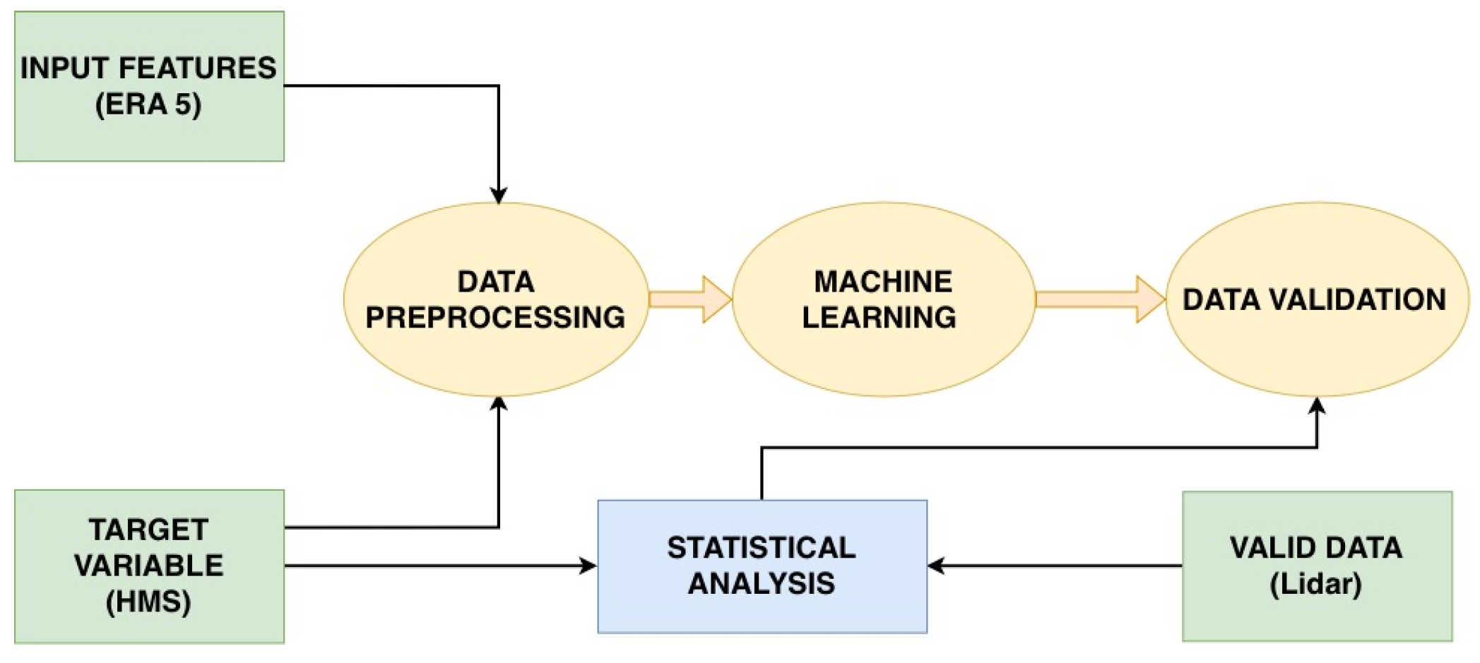
The methodology of this study is built upon a data partitioning strategy to ensure the reliable evaluation of high-level cloud (HLC) identification (see Figure 1). First, the training and internal testing phase utilized meteorological parameters (temperature, absolute and relative humidity, pressure, and wind direction and speed) derived from the ERA5 reanalysis data (Fifth Generation European Centre for Medium-Range Weather Forecasts Reanalysis) [51] as input features, with surface-based meteorological observations (presence/absence of HLCs) [52] serving as the target variable. Second, to assess the model’s reliability in a real-world experimental context, we employed atmospheric lidar sensing data. Crucially, the lidar data were not involved in the training process, providing an objective physical benchmark to verify the predictive accuracy and generalization capability of the trained ML models.

In accordance with the study’s conceptual framework two functionally distinct datasets were utilized. The first dataset, comprising 25,865 observations from meteorological stations and ERA5 reanalysis, served as the primary data for the training and internal testing of the ML models. The second dataset, consisting of 2258 ground-based lidar sensing observations, was employed strictly as an independent dataset for the external validation of the trained models. Within this set, 1476 cases were identified where lidar data and meteorological observations were fully synchronized in time. The integration of lidar sensing data necessitated a preliminary statistical analysis. The objective of this analysis was to confirm the feasibility of combining these diverse data types and to determine the conditions under which both experimental samples could be considered as drawn from the same population.

2.1. Data from the Hydrometeorological Station

In the study, the data from standard meteorological observations for the period 2010–2024 at the “Tomsk” Hydrometeorological Station (HMS) (ID 29430). The station is in the southwestern part of Tomsk, Russia (Tomsk Oblast), at coordinates 56°26′50″ N and 84°58′28″ E. Situated at an elevation of 141 m above sea level, the station is positioned on the right bank of the Tom River within the southeastern part of the West Siberian Plain. The data were obtained from the server of the Russian Research Institute of Hydrometeorological Information—World Data Centre (RIHMI–WDC) [52]. This data included information on cloud amount (total and low-level), morphological cloud types (families and forms), and atmospheric phenomena in the vicinity of the HMS, including information on the presence of various forms of HLCs and their combinations. Observations of clouds and phenomena at the “Tomsk” HMS are performed using visual–auditory methods every 3 h at standard synoptic times (00:00, 03:00, 06:00, 09:00, 12:00, 15:00, 18:00, and 21:00 UTC) [53]. The total cloud amount and the low-level cloud amount are determined as the fraction of the sky (on a 10-point scale) covered by clouds of all forms and by clouds of only the low-level and vertically developed families, respectively.

Only information regarding the presence and number of high-level clouds was utilized. Due to the absence of cloud base height measurement instruments (ceilometers) at the HMS, such data were not included in this study.

The presence of HLC (Cirrus, Cirrostratus, Cirrocumulus) at meteorological stations is determined by comparing the morphological characteristics of observed clouds (shape, texture, size, color, etc.) with the diagnostic features of specific cloud types [54]. Each major cloud genus has a unique set of diagnostic criteria, which minimizes the probability of error in visual identification. Cloud cover at meteorological stations is estimated as the fraction of the sky covered by all clouds or by clouds of a specific layer (including the high layer) and is expressed in oktas or tenths of the sky [55]. The error margin for this method does not exceed 1 okta (10%).

The distance between the HMS and ground-based lidar is less than 1 km, ensuring that the station data are representative of the study site. Data from other regional meteorological stations were not used, as the distance to them exceeds 50 km.

To exclude HLC passing at a distance from the lidar (i.e., those observed near the horizon), cases with cloud cover of less than 4 tenths were omitted. To verify the presence of high-level clouds over the study site, a comparison was performed between visual observations and lidar sounding data (Section 3.2).

2.2. Ground-Based Lidar Sensing Data

Lidar methods are the most promising for solving operational control and atmospheric monitoring tasks, as they provide real-time determination of the vertical profiles of atmospheric optical characteristics, microphysical parameters of clouds and aerosols, as well as some meteorological quantities. Furthermore, the use of polarized laser radiation and determining the polarization characteristics of radiation backscattered by the examined medium provides an estimate of its microstructural parameters. This idea is the basis of the design of the High-Altitude Matrix Polarization Lidar (HAMPL) developed at the National Research Tomsk State University (NR TSU).

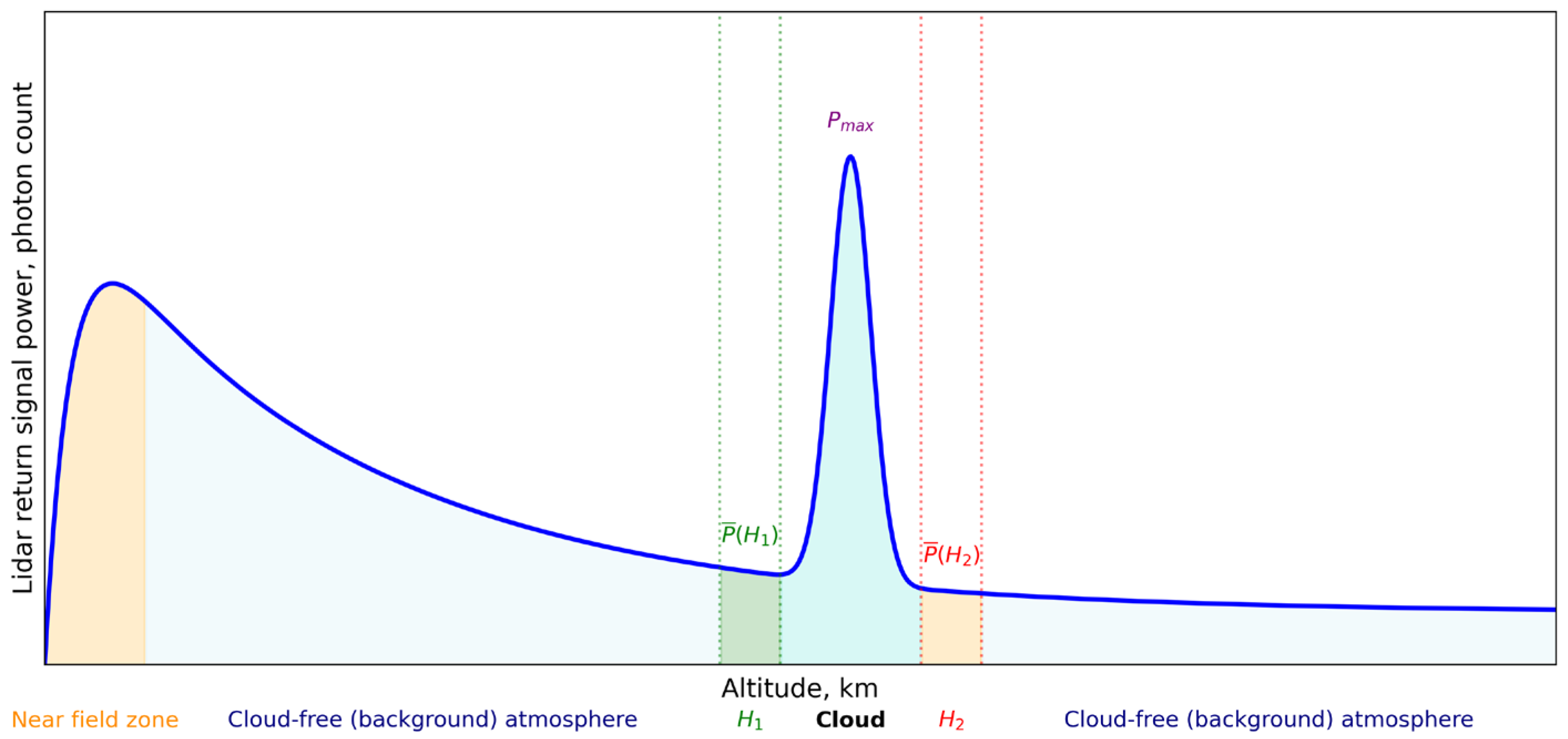
The method for estimating the lower boundary height H₁ is like that described in [56]. First, the pre-processed lidar return profiles are visualized using the developed software (Figure 2). Then, the operator visually identifies an altitude region in the sub-cloud layer where a change in the sign of the vertical gradient of the lidar return profile is observed and analyzes the sequence of signal power samples P(h_i) in this layer. After that, a pair of consecutive range gates, h_k and h_k+1, is selected such that in the second one (corresponding to a higher altitude) the lidar return value increases by more than 10% relative to the value in the previous range gate. The altitude h_k of the first of these range gates is taken as the location of the point where the vertical gradient of the lidar signal profile is zero. Then the height of the cloud base H₁ can be estimated as the average value of the altitudes of 4 consecutive range gates [57]:

H₁ = 1/4 (h_k + h_k–1 + h_k–2 + h_k–3)

(1)

This algorithm is adopted to exclude possible cases of false H₁ estimation when there is no cloud aerosol at that altitude, but only background aerosol characteristic of a cloud-free atmosphere. The height H₂ of the cloud top is determined in a similar manner, with the difference that for the considered pairs of adjacent range gates, the analysis focuses on the decrease in the lidar return [36].

To quantitatively characterize the scattering properties of particles in HLCs, the scattering ratio R is used. It is calculated as the ratio of the sum of the aerosol $\left({\beta }_{\pi }^a\right)$ and molecular backscattering coefficients ${\beta }_{\pi }^m$ to the latter: $R=({\beta }_{\pi }^m+{\beta }_{\pi }^a)/{\beta }_{\pi }^m$.

As a rule, the HLC thickness ΔH = H₂ − H₁ is small (ΔH/H₁ << 1), and the value of ${\beta }_{\pi }^m$ at the HLC upper and lower boundaries differs insignificantly (within 10%). Therefore, the parameter R can be estimated as the ratio of the maximum lidar return power P_max(h_m) from the cloud to the lidar return power P(H₁) from the atmospheric layer at the cloud lower boundary height H₁: $R=P_{\max }(h_m)/P\left(H_1\right)$ [36].

We can find the integral optical thickness of the cloud ${\tau }_h={\displaystyle \underset{H_1}{\overset{H_2}{\int }}\alpha (z)dz}$ using the lidar sensing equation:

$${\displaystyle \frac{P\left(H_2\right)}{P\left(H_1\right)}}={\displaystyle \frac{{\sigma }_{\pi }\left(H_2\right)H_1^2}{{\sigma }_{\pi }\left(H_1\right)H_2^2}}{e}^{-2{\tau }_h}$$

(2)

As mentioned above, for HLCs the relation ΔH/H₁ << 1 holds true. Therefore, it can be assumed that ${\tau }_h={\displaystyle \underset{H_1}{\overset{H_2}{\int }}\alpha (z)dz}$, and then the estimation of τ_h simplifies to:

$${\tau }_h\approx {\displaystyle \frac{1}{2}}\ln {\displaystyle \frac{P\left(H_1\right)H_1^2}{P\left(H_2\right)H_2^2}}$$

(3)

Clouds with predominantly horizontally oriented ice particles (specular clouds) are identified [55,56,57] according to the criterion: scattering ratio R ≥ 10, optical thickness τ_h ≤ 1, and the backscattering phase matrix element m₄₄ ≤ –0.4.

2.3. Predictive Models for HLC Identification

While previous studies [19,20,21,22,23] primarily focused on image segmentation and cloud detection using computer vision techniques (e.g., FCN and CNN), our research adapts the core machine learning principles to tabular geophysical data. Instead of analyzing spatial patterns from satellite or ground-based imagery, we focus on identifying complex thermodynamic relationships between vertical atmospheric profiles (from ERA5) and HLC occurrence. This approach allows for a physical interpretation of cloud formation conditions rather than just visual identification. Our validation approach follows the methodology established in recent studies, such as [58], where high-precision lidar data (CALIOP) is used as the ‘ground truth’ to evaluate machine learning models based on atmospheric observations. Similarly, we employ ground-based lidar sensing to independently verify the accuracy of our ML-based HLC identification. Ref. [59] have demonstrated that machine learning algorithms, specifically gradient boosting decision trees (GBDT), significantly outperform traditional threshold-based methods in cloud detection. Following this approach, we utilize XGBoost to capture the complex relationships between vertical atmospheric profiles and HLC occurrence. The choice of XGBoost, LightGBM, and CatBoost for HLC identification is driven by their efficiency in modeling non-linear dependencies and feature interactions in tabular geophysical data [60,61,62].

Cloud Detection Assessment Metrics

Evaluation metrics are crucial for accurately assessing the effectiveness of cloud detection models. In this work, the HLC detection was considered as a classification task using standard evaluation metrics: True Positives (TPs), True Negatives (TNs), False Positives (FPs), and False Negatives (FNs). Derived metrics such as Precision (P) and Recall (R) were also used. Furthermore, ROC curves and the F1-score were analyzed. These metrics are calculated as follows:

P = TP/(TP + FP)

(4)

R = TP/(TP + FN)

(5)

F1 score = 2(P × R/(P + R))

(6)

For calculating the area under the ROC curve, numerical methods such as the trapezoidal rule, which integrates the TP values at various threshold levels arranged in ascending order of FP rates are typically used. Overall, the ROC curve is a numerical metric that takes a value in the range from 0 to 1: the closer it is to 1, the better the model, as it more effectively separates the classes.

2.4. Statistical Methodology for Data Consistency Assessment

To test the hypothesis of independence between the surface-based meteorological observations and lidar sensing data, the Pearson’s chi-squared (χ²) test was implemented [63]. The null hypothesis (H₀) was formulated as follows: the two types of observations are independent of each other. Under this assumption, the test statistic (Equation (7)) calculated from the contingency table (see Section 3.2) follows a distribution with the appropriate number of degrees of freedom. This test allowed us to determine whether the lidar measurements and meteorological reports can be considered as representing the same atmospheric phenomena.

$${\chi }^2=\sum _{i,j}{\displaystyle \frac{{\left(O_{i,j}-E_{i,j}\right)}^2}{E_{i,j}}},$$

(7)

where O_ij is the observed frequency of the two different HLC detection methods (0—not observed, 1—observed), and E_ij is the expected frequency under the assumption of independence. In this case, the number of degrees of freedom is 1. If the calculated χ² value exceeds the critical value, the null hypothesis (H₀) is rejected, indicating a statistically significant association between the datasets. Furthermore, to quantify the strength of this relationship, the odds ratio (OR) test was implemented [63]. The OR is a measure of association that quantifies the odds of HLC detection by one method (e.g., lidar) given the presence of HLC according to the other method (meteorological observation). The formula for the odds ratio used in this study is as follows:

$$OR={\displaystyle \frac{O_{00}\cdot O_{11}}{O_{01}\cdot O_{10}}},$$

(8)

where (1, 1) represents cases where both methods detected clouds, (0, 0) denotes cases where both methods did not detect clouds, and (0, 1) and (1, 0) represent discrepancies between the two methods.

If our observations are not independent, we need to check hypothesis that both datasets are drawn from the same general distribution. Under this assumption, the statistic is calculated as follows:

$${\chi }^2={\displaystyle \frac{{\left(l_0-m_0\right)}^2}{m_0}}+{\displaystyle \frac{{\left(l_1-m_1\right)}^2}{m_1}},$$

(9)

where l₀ and l₁ represent the observed frequencies of cloud presence and absence detected by the lidar, respectively, while m1 and m0 denote the corresponding observed frequencies from the meteorological observations. The procedure of test as same as above.

3. Results

To solve the problem of predicting the HLC detectability, a preliminary analysis of meteorological data was performed. The initial data are presented in the form of a feature table derived from the ERA5 climate reanalysis and observations, including parameters such as temperature, relative and absolute humidity, pressure, and wind speed. A distinctive characteristic of the meteorological data used is their vertical organization: atmospheric parameters are presented as vertical profiles from the Earth’s surface up to an altitude of 14,000 m with a step of 500 m.

It should be noted that in the initial ERA5 reanalysis data, vertical levels are specified not by geometric height, but in pressure coordinates (isobaric levels). For the purposes of analysis and visualization, the data were converted to a height scale using the standard barometric formula: Z = RT/g ln(p₀/p), where Z is the height (in meters), R is the universal gas constant for air, (R≈8.314 J/(mol·K)), T is the absolute temperature (in Kelvin), g is the acceleration due to gravity (approximately 9.80665 m/s²), p₀ is the standard or reference sea-level pressure (typically 1013.25 hPa or 101,325 Pa), and p is the pressure at the considered level (Pa).

Since the original data dimensionality makes direct analysis challenging, it was decided to aggregate the meteorological parameter values within the altitude range of 6000 to 12,000 m—it is at these altitudes, according to observations, that HLCs are most frequently form. Thus, the subsequent analysis was performed on the averaged feature values within this atmospheric layer.

3.1. Data Preprocessing and Visualization

At the initial stage, data loading and preliminary verification were performed: analysis of the table structure, assessment of missing values, and examination of the target feature distribution (presence or absence of HLCs). After preliminary cleaning and removal of invalid entries, aggregated values for the specified altitude interval were calculated, and the data were prepared for visualization.

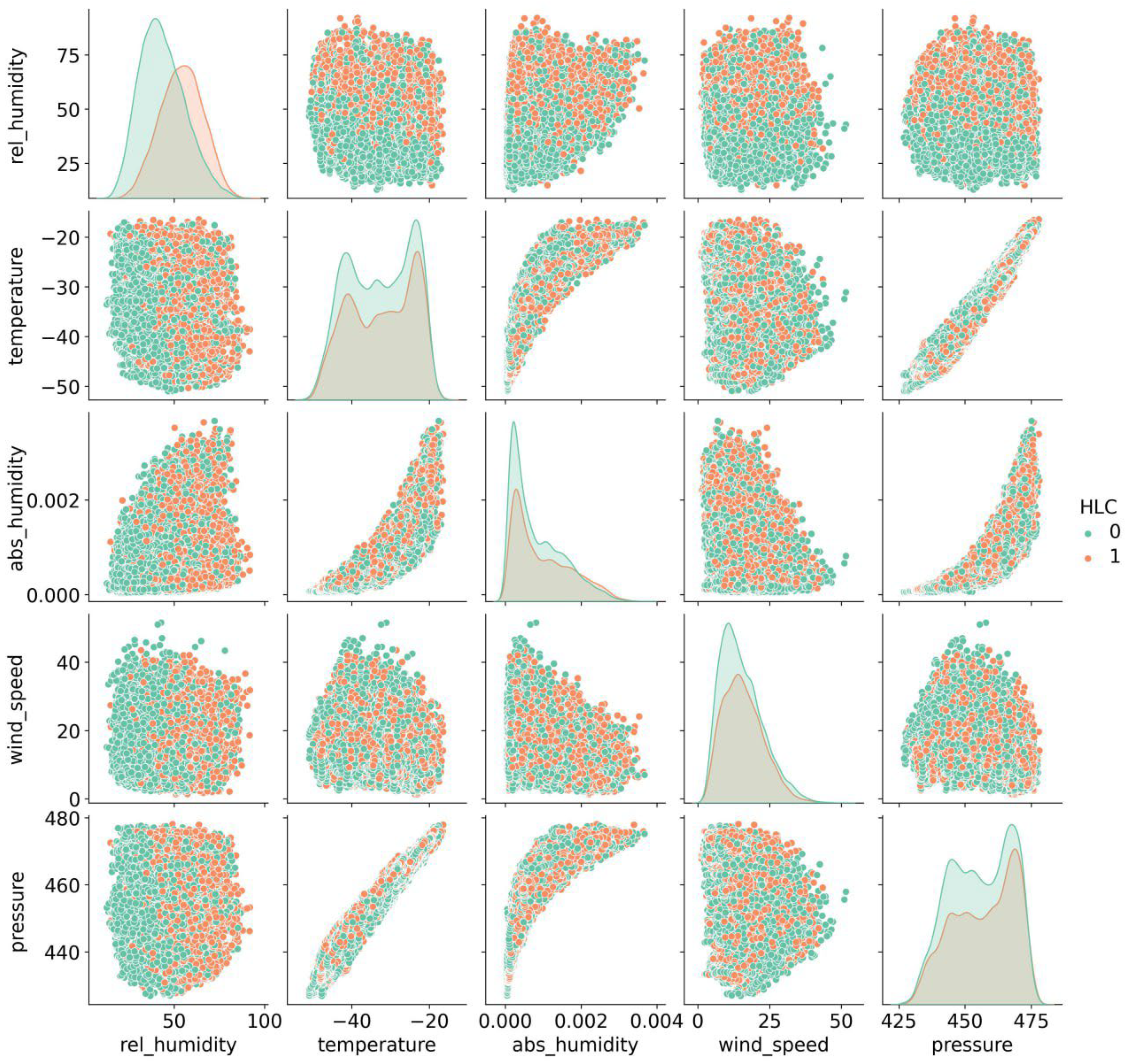
Figure 3 presents a pairplot, where each point corresponds to an averaged observation for a single case. Color coding reflects class membership—the presence (red) or absence (green) of HLCs.

An understandable physical relationship among temperature, absolute humidity, and relative humidity (as air temperature increases, its capacity to hold moisture in absolute terms rises, while relative humidity may decrease) is observed. The classes of hydrometeorological conditions are not strictly separated by any single specific meteorological parameter; however, shifts in mean values (for wind speed, temperature, and humidity) are apparent. These shifts are not pronounced enough to visually separate the set, but they indicate that when accounted for multifactorially (within a model), they can indeed be used for classification.

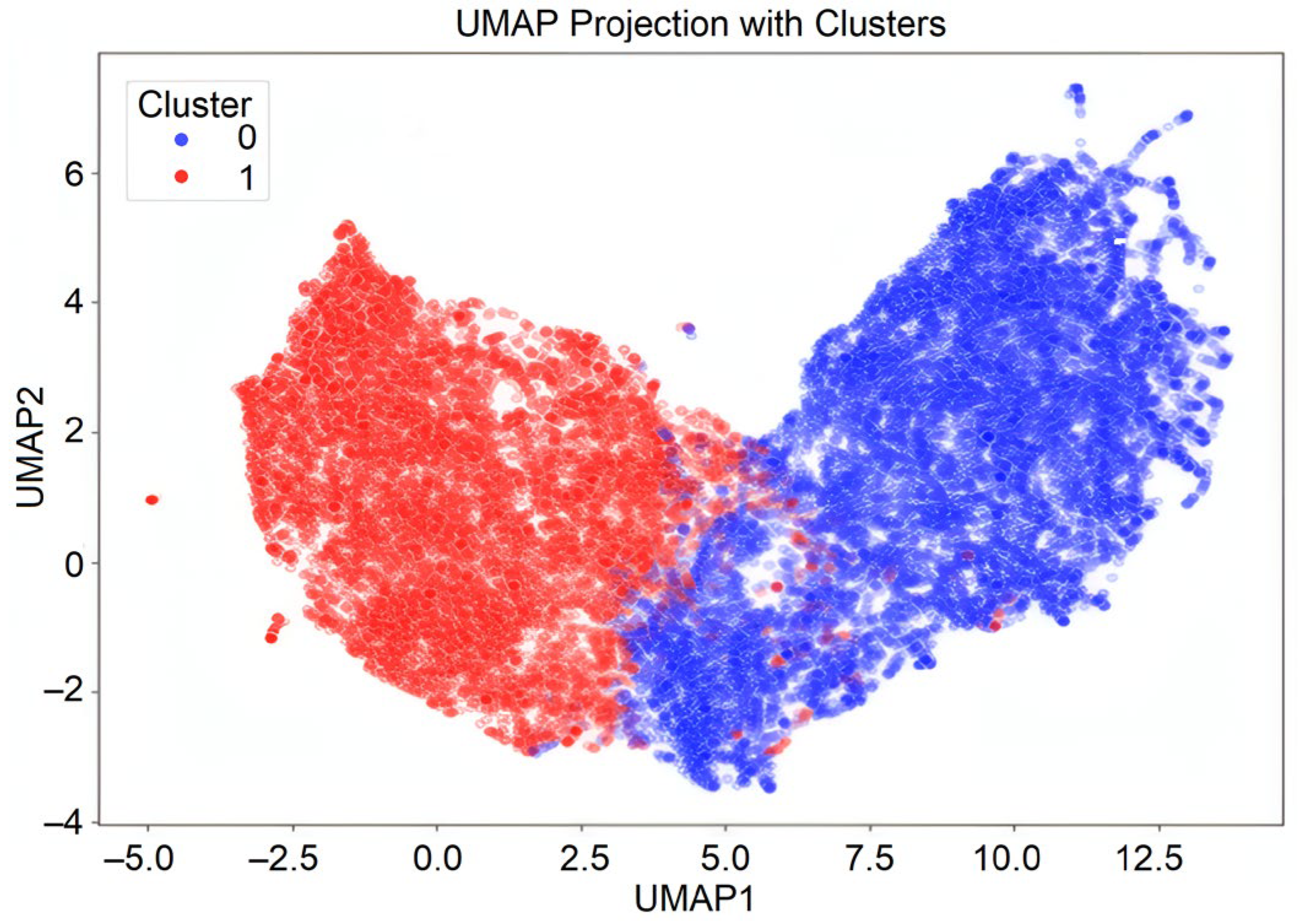
To analyze the multidimensional structure of the data and potential clustering, the UMAP algorithm, which allows the data to be visualized in two-dimensional space, was applied. The resulting projections showed a reasonably clear separation between observations with and without HLCs, further confirming the distinction between the classes.

The UMAP visualization, presented in Figure 4, shows that the observations form two well-distinguished clusters, color-coded for clarity. The blue and red clusters (Cluster 0 and Cluster 1) correspond to the data for the absence and presence of HLCs, respectively. A clear separation between the clusters is evident, despite a slight area of overlap between them.

This indicates the existence of two distinctly different atmospheric states that correspond to the absence and presence of HLCs. The clear separation in the feature space demonstrates that the used meteorological parameters are indeed sensitive to the physical differences between these atmospheric states, making them promise for further prediction of HLC formation probability.

3.2. Investigation of the Possibility of Simultaneous Use of Meteorological Observations and Lidar Sensing Data

Data collection and preparation from the HMS for the period from 2010 to 2024 were implemented [52]. The data were collocated in place and time with the lidar experiment. The data meet the established accuracy criteria for time, while different thresholds were considered depending on the state of ground-based observations. The specific thresholds are as follows: for observations with a start altitude of less than 8000 m (the conventional boundary for the formation of cirrostratus and cirrocumulus), a deviation of up to 3720 s (approximately 62 min) is allowed, and for observations with a start altitude of 8000 m and above (primarily cirrus), a twofold smaller deviation is allowed—up to 1920 s (approximately 32 min). The logic for selecting the time thresholds was as follows: cirrus has a complex structure and consists of individual cloud elements with gaps in between. If the time interval exceeds half an hour, the data becomes unrepresentative. At the same time, cirrostratus is more homogeneous and spread over large distances (up to hundreds of kilometers), so the time interval increased to one hour [1,55]. While atmospheric conditions can fluctuate within an hour, especially with the strong wind, the threshold of 62 min was selected based on the typical horizontal scale, which can easily reach more than a thousand kilometers.

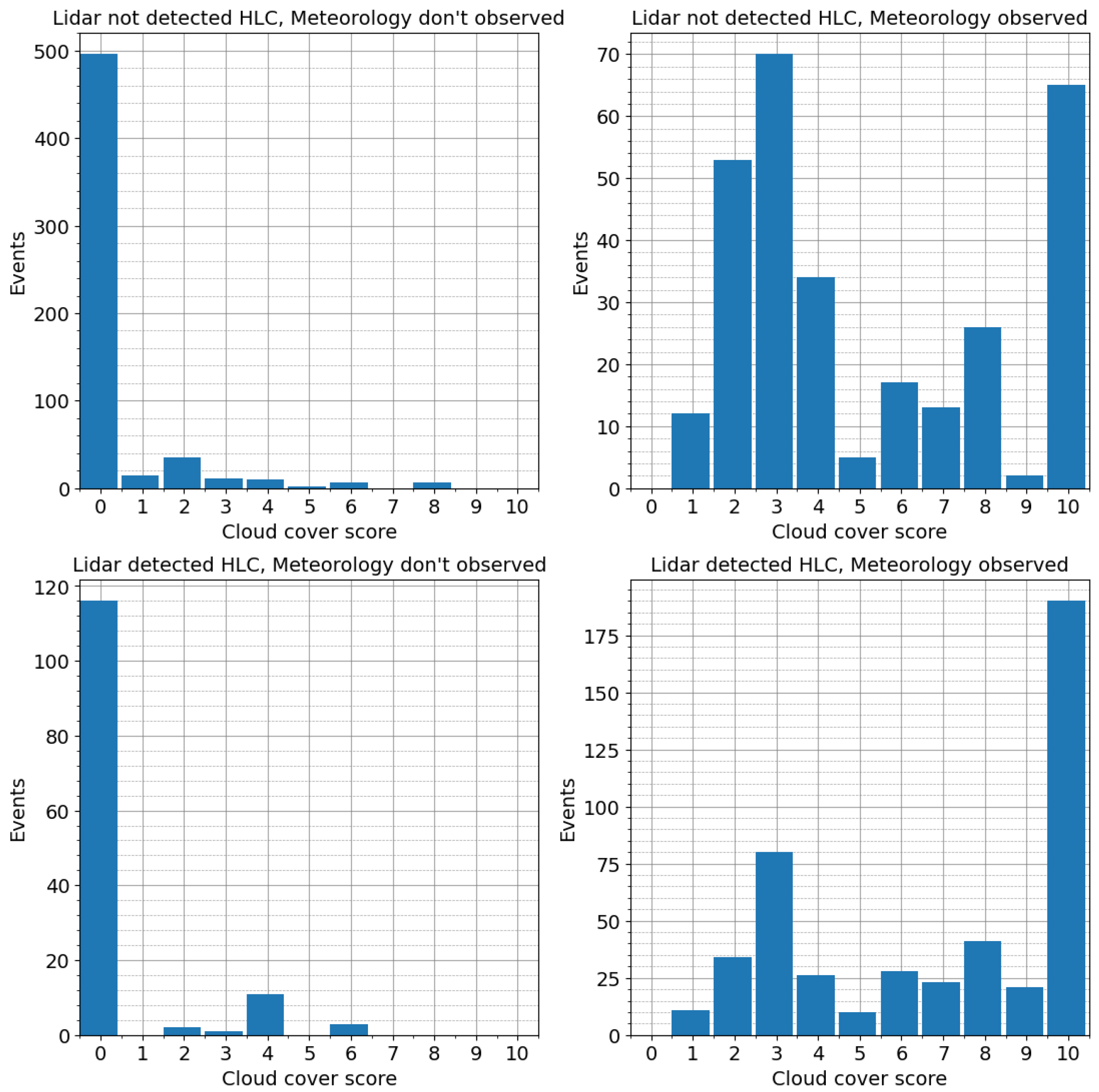
Total cloud amount characterizes the degree of sky coverage by clouds and is expressed as a numerical estimate. In meteorology, cloud amount is measured in tenths, where one tenth corresponds to one-tenth of the sky, and oktas are also used, each corresponding to one-eighth of the celestial sphere. Detailed studies of atmospheric sensing data and observations at the HMS have shown that the lidar has greater sensitivity for registering HLCs and detects their presence at low cloud amounts, which a meteorologist cannot do visually (Figure 5). However, the lidar registers HLCs located strictly vertically within a narrow Field of View (FOV) at a 90° angle. Meteorologists’ observations include data on the presence of HLCs, including when they are located on the periphery of the sky.

In cases where the lidar registered HLCs but meteorologists did not observe them (133 cases), the cloud amount was very low (0.52), indicating sparse cloudiness or localized HLCs that meteorologists failed to record. This result can be explained by two main reasons: first, the lidar is a more advanced sensor. It can detect weak backscatter signals from cloud particles (crystals) at very low concentrations, which are indistinguishable to the human eye. Second, imperfections in the observation methodology at meteorological stations. According to the guiding documents of Roshydromet/WMO, during cloud observations at meteorological stations, observer-meteorologists do not record (do not enter the database) clouds (including HLCs) with an amount score of less than 1 (less than 10% of the sky). Thus, a cloud amount score of 0 indicates either a complete absence of clouds or a cloud cover of less than 1/10 of the sky.

In cases where meteorologists observed HLCs but the lidar did not (297 cases), the cloud amount score was high (5.25). Under broken or scattered cloudiness, the laser beam may pass through gaps between individual cloud elements due to the narrow spatial sampling of the zenith-pointing sensor, and as a result, the lidar fails to register the HLCs. The coincidence of observations (464 cases) is associated with a high cloud amount score (6.94). The absence of HLCs in both observation methods (582 cases) corresponds to a low cloud amount score (0.44). The results are presented in

Table 1. Numerical description of situations during HLC registration by two sources: Tomsk Meteorological Station and HAMPL.

Situation	Number of Cases	Mean Cloud Amount Score	Description (Total Amount of Cloud Cover)
Lidar YES/Meteorologists NO	133 (9%)	0.52	2 and below—118 measurements
Lidar NO/Meteorologists YES	297 (20%)	5.25	5 and above—128 measurements, 4 and below—169 measurements
Lidar YES/Meteorologists YES	464 (31%)	6.94	5 and above—313 measurements, 4 and below—151 measurements
Lidar NO/Meteorologists NO	582 (40%)	0.44	5 and above—15 measurements, 4 and below—567 measurements

.

The first stage of the analysis involved testing for dependence between observations obtained by different measurement methods. To assess the relationship between meteorological observations and lidar sensing data, two statistical tests were applied: Pearson’s χ² test for contingency tables and the calculation of the Odds Ratio [63].

To construct the contingency table based on the meteorological set, observations closest in time to the lidar measurements were selected (according to the temporal criteria specified earlier). As a result, two sets of 1476 observations each were formed: one meteorological and one lidar. Both sets contain binary features reflecting the absence or presence of HLCs at the corresponding time. A contingency table, displaying the number of coincidences and discrepancies between meteorological assessments of HLC presence and the results of lidar sensing (

Table 2. Contingency table of lidar and meteorological observations for HLCs, where 0 indicates absence, and 1 indicates presence.

Observations	Meteo_0	Meteo_1
Lidar_0	582	297
Lidar_1	133	464

), was then constructed. This allows for a statistical evaluation of the relationship between the two HLC identification methods and for determining whether the data obtained by two independent observation methods are dependent on each other.

Based on the methodology described in Section 2.4, the calculated χ² (Equation (7)) is 245.7. The critical value of χ² at a significance level of α = 0.01 is 6.635. Therefore, based on Pearson’s chi-squared test, the null hypothesis is rejected, indicating a statistically significant dependence between the two datasets.

The obtained OR value of 15.47 (Equation (8)) indicates that the odds of the observations matching are 15.47 times higher than the odds of them not matching. The statistical significance of this result is confirmed by the 95% confidence interval for the odds ratio [15.15, 15.76], which does not include the value of 1. This means that the result is statistically significant and further demonstrates a strong association between the measured features.

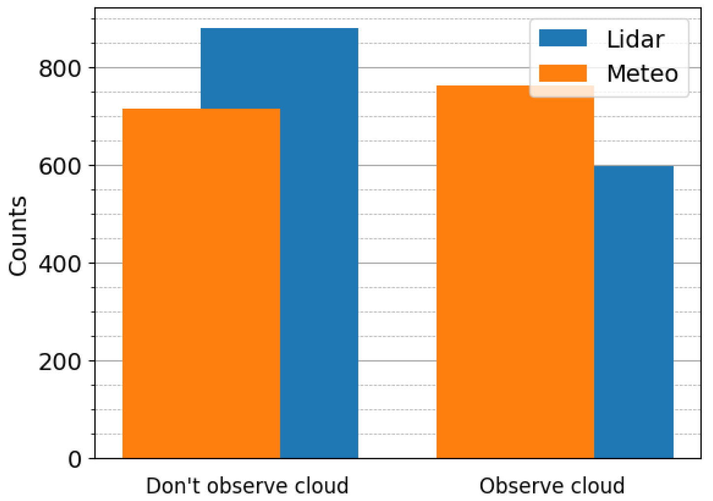
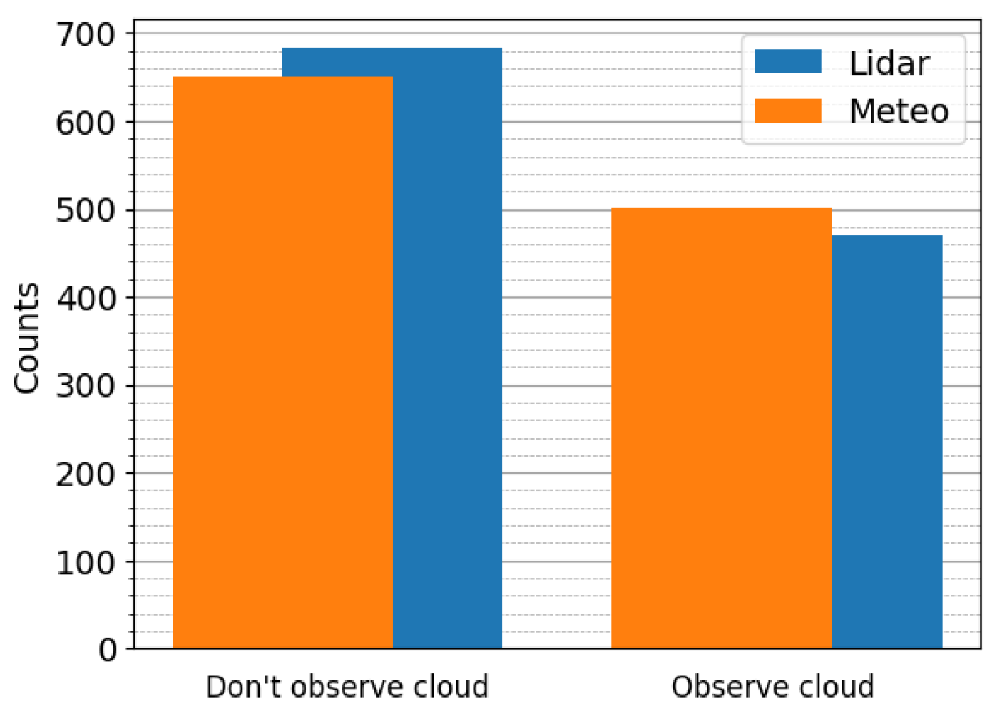
Finally, to determine whether the two datasets belong to the same distribution, Pearson’s χ² goodness-of-fit test was used [63]. The test is based on comparing the observed frequencies from one detection method with the observed frequencies obtained by the other method under the assumption of H₀. The visualization of the distributions is presented in Figure 6. The histograms are constructed based on the observed values, allowing a visual assessment of the degree of overlap. The performed analysis combines statistical evidence of both dependency and distribution similarity, which is important for interpreting and drawing further conclusions about the relationship between the measurements.

However, the data can be adjusted to make the distributions match. For this purpose, a filter based on cloud amount scores is applied. Only observations where the cloud amount score is 0 (less than 10% of the sky is covered) or greater than or equal to 4 (more than 40% of the sky is covered) are retained. These threshold values were determined through an optimization process to ensure maximum sample size while maintaining statistical homogeneity of the distributions. The visualization of the probability distributions for detecting HLCs by different methods using the presented filters is shown in Figure 7.

The difference in height between the orange and blue bars corresponding to the different methods of HLC detection has decreased. The calculated χ² value is 3.61, meaning that at the specified significance level, there is no statistically significant difference between the sets.

3.3. Development of an ML Model for Predicting the Absence and Presence of HLCs

The following meteorological parameters were used as input features: temperature, relative and absolute humidity, pressure, and wind speed. The presence of HLCs was encoded as a binary variable (0—absence, 1—presence). The model was trained on meteorological observation data. When preparing data for training ML models, the specifics of each algorithm were considered. Feature scaling was implemented for distance-based and linear methods, such as SVM, k-Nearest Neighbors (k-NN), and logistic regression. For this purpose, Standard Scaler and Principal Component Analysis (PCA) methods were used.

The initial dataset was split in a 70/15/15% ratio, where 70% was used for model training, 15% for validation, and the remaining 15% served as the control set, defined as the last values in the overall dataset. The validation set was used for hyperparameter tuning, while the control set was used to evaluate the model’s accuracy and quality. This approach allows for considering current conditions and dynamic parameter changes, ensuring a more relevant model evaluation and testing its ability to correctly predict the absence/presence of HLCs in real weather situations. Furthermore, verification of the developed model was performed using experimental data obtained from atmospheric lidar sensing to assess its applicability in real monitoring conditions. A hyperparameter search approach was used for feature engineering, followed by training the final model. This enhances the model’s generalization ability, improving its accuracy and robustness.

The article presents the results of the top three models (

Table 3. Comparison of ML model performance metrics for the HLC presence/absence using the standard meteorological observations and lidar sensing data.

Model	Absence (Class 0)/Presence (Class 1) of HLC	Meteorology				Lidar
		ROC AUC	Precision	Recall	F1	ROC AUC	Precision	Recall	F1
XGBoost	0	0.88	0.8410	0.7428	0.7889	0.78	0.8282	0.7281	0.7749
	1		0.7537	0.8486	0.7984		0.6121	0.7396	0.6698
CatBoost	0	0.88	0.8351	0.7635	0.7977	0.77	0.8127	0.7538	0.7821
	1		0.7666	0.8375	0.8005		0.6227	0.7005	0.6593
LightGBM	0	0.87	0.8389	0.7546	0.7946	0.78	0.8180	0.7266	0.7696
	1		0.7613	0.8438	0.8005		0.6048	0.7214	0.6580

), among which the models based on gradient boosting (over decision trees) proved most successful.

Their selection is justified by high accuracy, stability, good performance with tabular data, and effectiveness in classification tasks, ensuring a balance between prediction precision and recall. In the present study, the effectiveness of ML models for classifying the absence/presence of HLCs based on meteorological parameters and atmospheric lidar sensing data was evaluated. For determining the absence of HLCs (class 0), the XGBoost model proved to be the most effective when analyzing meteorological observations, achieving a binary classification model performance of 0.88 (ROC AUC), a proportion of correctly classified instances among all instances of 85% (Precision, Formula (4)), and a proportion of correctly identified instances of the negative class among all actual cases of that class of 75% (Recall, Formula (5)). This model also demonstrated robustness when validated on real experimental atmospheric lidar sensing data. Similar robustness was shown by the LightGBM and CatBoost models when using both meteorological and lidar data.

When classifying the presence of HLCs (class 1), the performance metrics show some decline, particularly for models validated on real lidar data. This is due to differences in HLC registration by each method: the lidar detects clouds in the zenith, located strictly vertically at a 90° angle, while meteorological observations account for cloud presence across the entire sky, including its periphery. Such data creates disparities in feature characteristics, which affects the effectiveness of the methods. Specifically, integral characteristics representing large areas are better predicted by ML methods than localized fluctuations associated with the restricted zenithal FOV of lidar measurements. This is especially relevant for inhomogeneous clouds, such as cirrus, with complex structures consisting of individual elements and gaps. These specific features explain the decrease in classification accuracy, particularly under conditions of high cloud structural complexity.

Models trained on meteorological data demonstrate a stable ROC AUC of 0.87–0.88, while Precision varies within the range of 76–77% and Recall within 84–85%. The harmonic mean between Precision and Recall—the F1-score (Formula (6))—shows relatively stable and balanced performance: 77–78% for class 0 and 66–68% for class 1. Specifically, the XGBoost and CatBoost models exhibit higher metrics, indicating the ability to predict both cloud conditions while minimizing both false positives and missed cases. 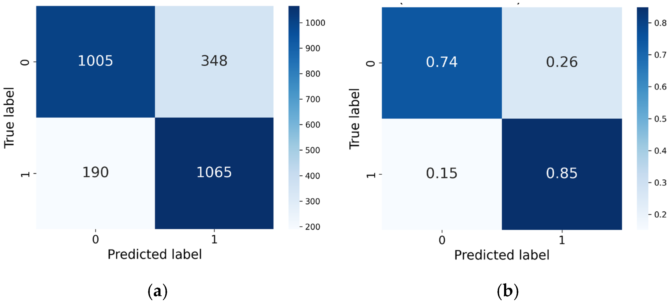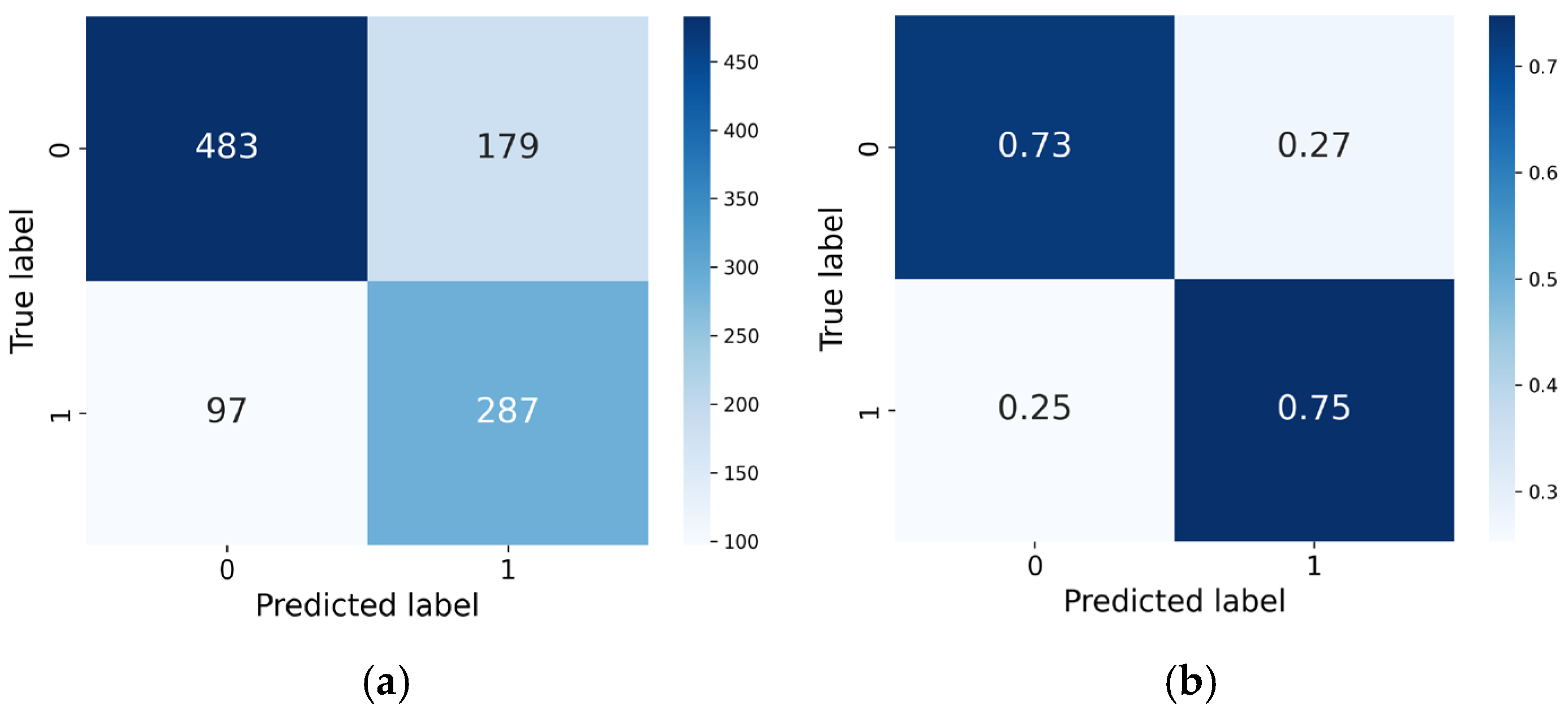Figure 7 (meteorological data) and 8 (lidar sensing data) present confusion matrices for the XGBoost method in two forms: as absolute counts (Figure 8a and Figure 9a) and as row-normalized values (Figure 8b and Figure 9b).

Absolute values show the exact number of instances for each combination of the true and predicted class, allowing for an assessment of the model’s numerical errors. In other words, they show how many times the model correctly predicted the absence of HLCs and their presence, as well as how many cases were erroneous. Row-normalized values demonstrate the relative proportions of errors and correct predicts within each true class, which facilitates model comparison across different classes and allows for accounting for class imbalance. The use of both forms provides a more comprehensive understanding of the model’s performance: absolute metrics demonstrate the actual quantities of errors, while normalized ones show its effectiveness under different data distributions.

The performance metrics of the evaluated machine learning models are summarized in

Table A1. Comparison of ML model performance metrics for the HLC presence/absence using the standard meteorological observations and lidar sensing data.

Model	Absence (Class 0)/Presence (Class 1) of HLC	Meteorology				Lidar
		ROC AUC	Precision	Recall	F1	ROC AUC	Precision	Recall	F1
XGBoost	0	0.88	0.8410	0.7428	0.7889	0.78	0.8282	0.7281	0.7749
	1		0.7537	0.8486	0.7984		0.6121	0.7396	0.6698
CatBoost	0	0.88	0.8351	0.7635	0.7977	0.77	0.8127	0.7538	0.7821
	1		0.7666	0.8375	0.8005		0.6227	0.7005	0.6593
LightGBM	0	0.87	0.8389	0.7546	0.7946	0.78	0.8180	0.7266	0.7696
	1		0.7613	0.8438	0.8005		0.6048	0.7214	0.6580
SVM-RBF	0	0.86	0.8260	0.7369	0.7789	0.77	0.7886	0.7946	0.7916
	1		0.7459	0.8327	0.7869		0.6412	0.6328	0.6370
Log-reg	0	0.83	0.7901	0.7539	0.7716	0.72	0.7316	0.7825	0.7562
	1		0.7472	0.7841	0.7652		0.5740	0.5052	0.5374
Gaussian-NB	0	0.82	0.8078	0.6741	0.7349	0.73	0.7886	0.6707	0.7249
	1		0.7018	0.8271	0.7593		0.5487	0.6901	0.6113
kNN	0	0.83	0.7957	0.7398	0.7668	0.77	0.8239	0.7704	0.7963
	1		0.7393	0.7952	0.7662		0.6440	0.7161	0.6782

(Appendix A). While we primarily report results for XGBoost, it should be noted that modern gradient boosting frameworks—including LightGBM and CatBoost—yielded comparable predictive performance during our tests. These implementations share similar underlying principles, and any of them can be effectively utilized for HLC identification with consistent accuracy. The choice of XGBoost for the final analysis was based on its widespread adoption in atmospheric studies and its robust handling of sparse meteorological features.

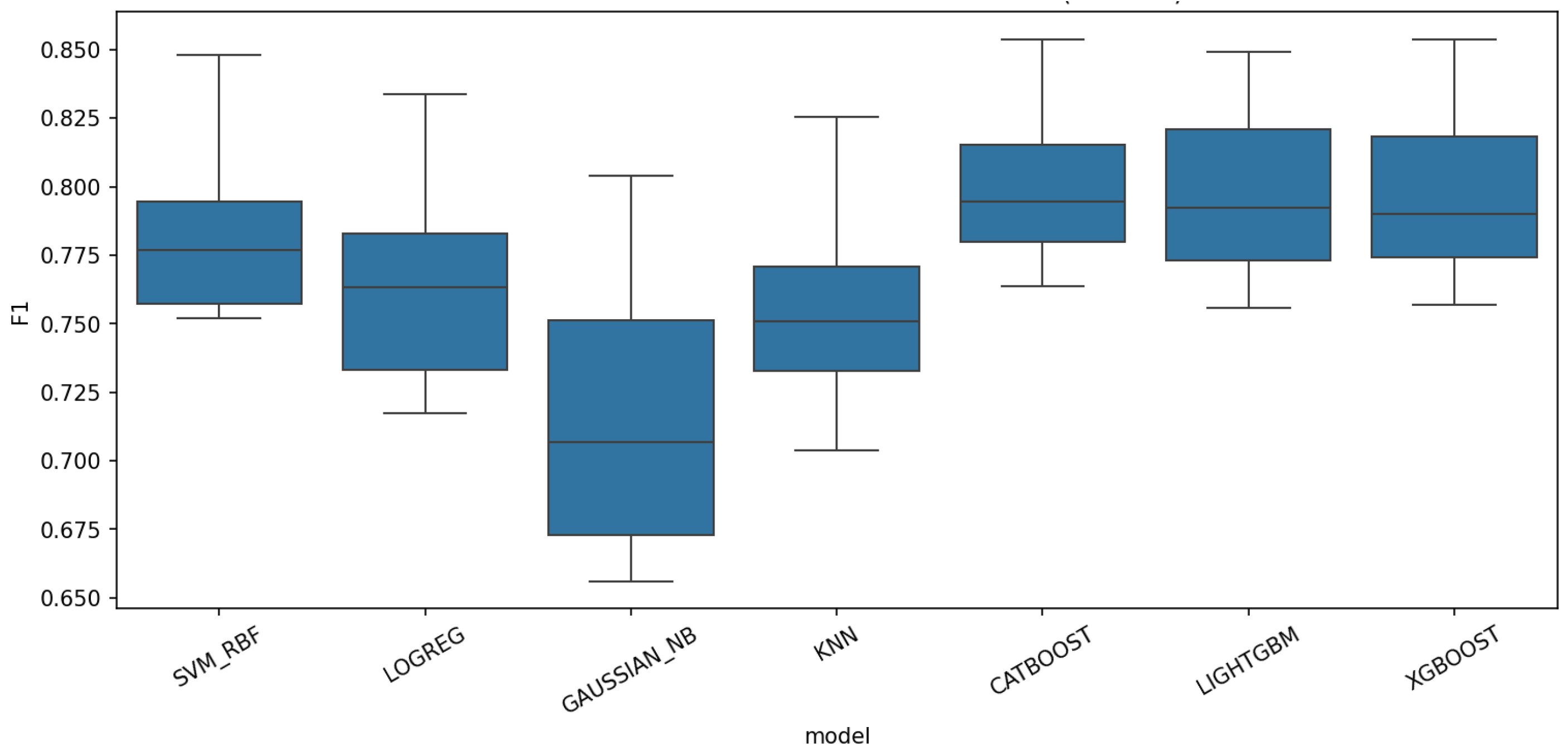
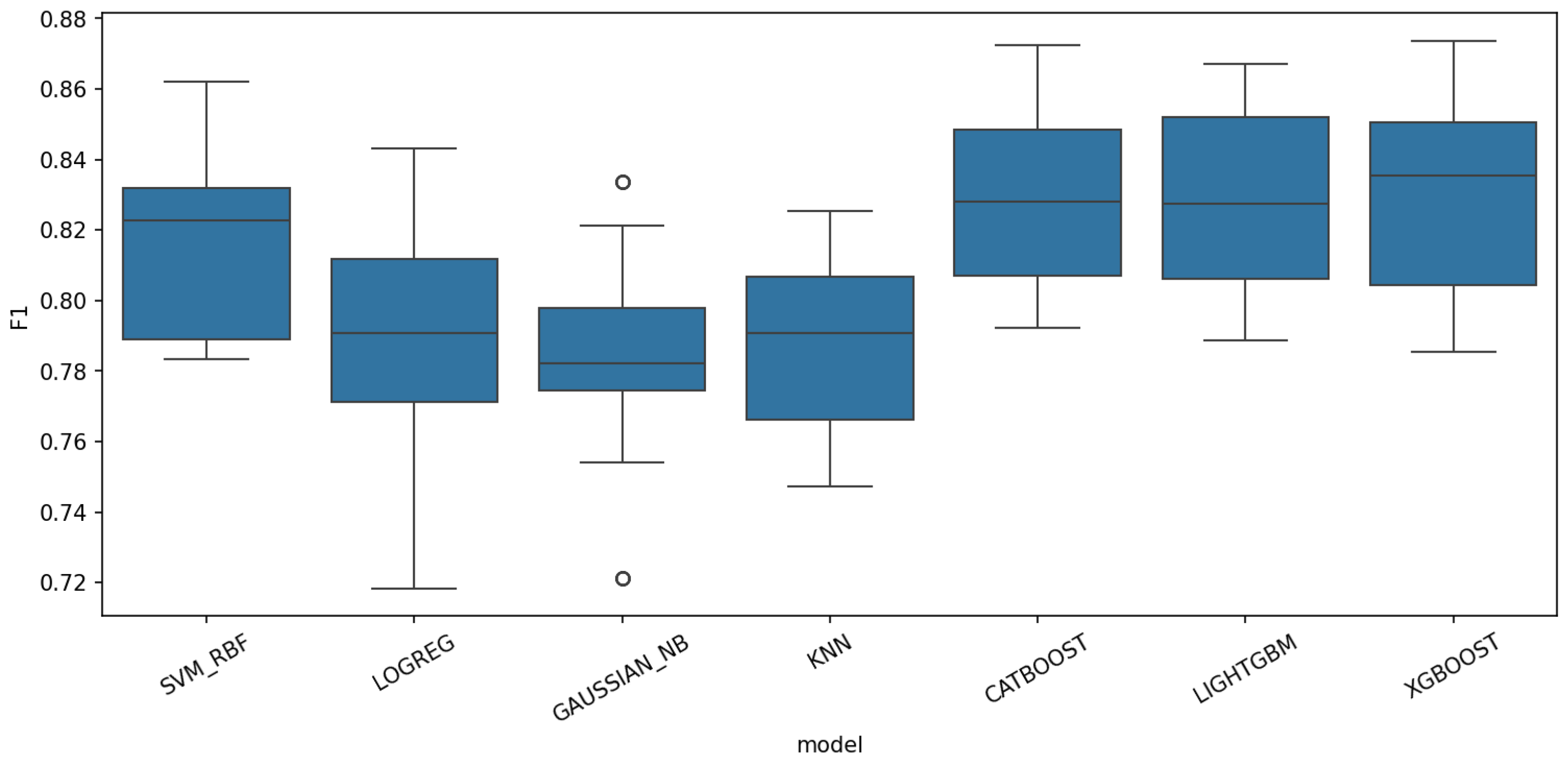
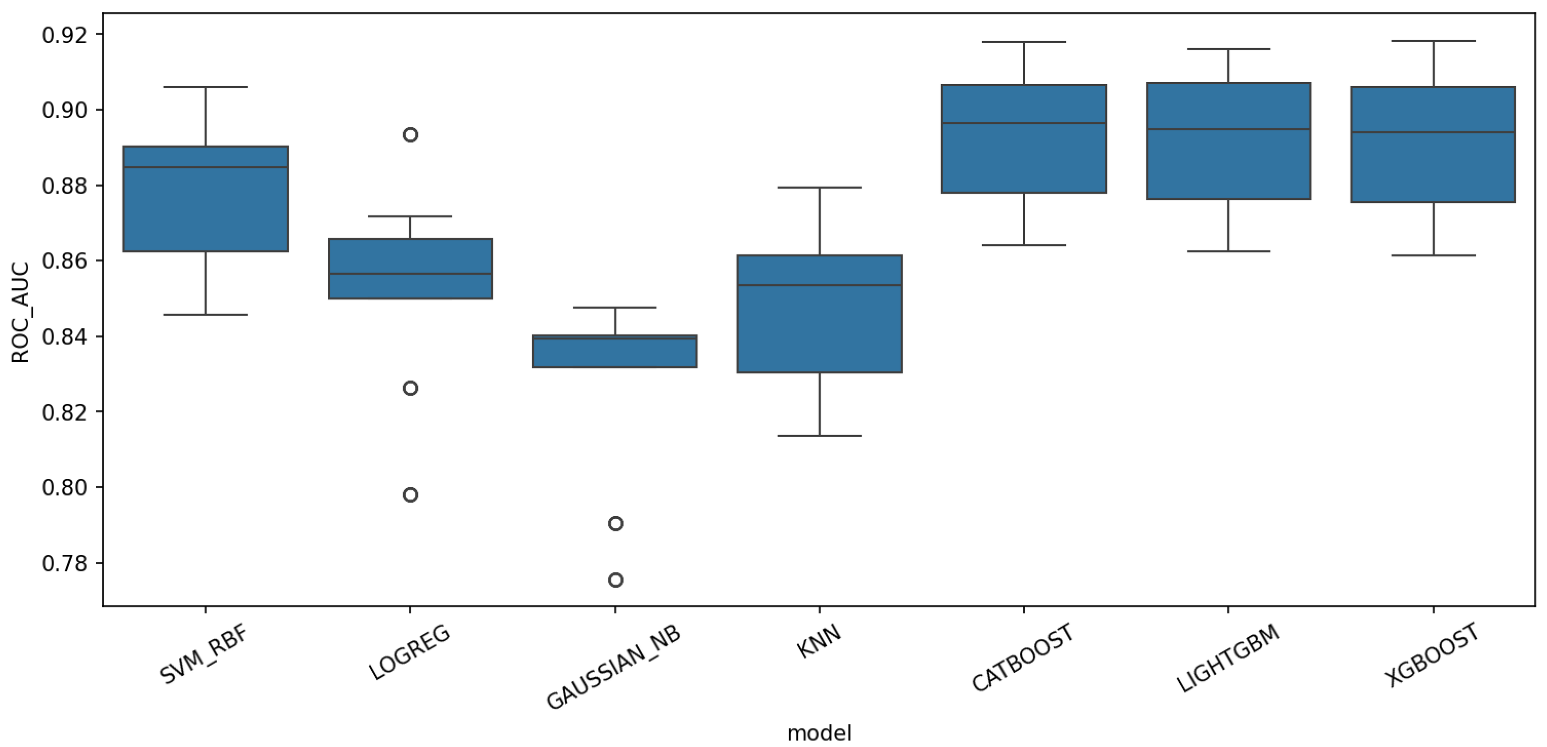
To evaluate model stability and the sensitivity of the results to random data partitioning, cross-validation was employed. The experimental setup utilized a scheme with k = 10 folds and 5 repetitions, resulting in 50 independent training and testing iterations for each of the seven algorithms (totaling 350 cycles). At each stage, a new split was performed, and the random_state parameter was varied to account for both the impact of random sampling and the internal stochasticity of the learning algorithms. For each iteration, ROC-AUC, Precision, Recall, and F1-score metrics were calculated. Visualizations of these distributions are provided in Appendix A, Figure A1, Figure A2 and Figure A3. The use of boxplots enables a clear comparison between the models: a narrow range of values indicates high stability, whereas the presence of outliers or a wide spread suggests sensitivity to variations in the training data and potential instability in the model’s generalization capacity.

4. Existing Issues and Future Directions

The study was conducted in Tomsk, located in the southeastern part of the West Siberian Plain. This region is one of the world’s largest lowland plains, situated in temperate latitudes and characterized by flat terrain with minimal elevation variations (0–200 m). Climatic conditions across this territory are relatively homogeneous and change gradually in the latitudinal direction. Consequently, our findings and derived thresholds are representative of a significant portion of this region, excluding its northern polar areas. Furthermore, the developed methodology and model are potentially applicable to other global regions with similar physiographic and continental climatic conditions. However, we acknowledge that in regions with significantly different characteristics (e.g., tropical latitudes or mountainous terrain), the model parameters may require recalibration to account for different cloud base heights and atmospheric profiles.

By organizing and summarizing the tasks related to the detection of HLCs and their subsequent processing using classical ML methods, the potential for the combined use of meteorological observation data and lidar sounding becomes evident, promising improved accuracy in estimating the probability of HLC occurrence. Current research has focused on evaluating the effectiveness of various ML algorithms and identifying key features that influence the likelihood of HLC formation. There has also been interest in exploring the relationship between meteorological conditions and HLC emergence—determining patterns that could be used to enhance predicts and identify the most robust and accurate algorithms under different conditions. At the same time, several challenges in the developed HLC detection methods have been identified that require further investigation. First, the acceptable levels of cloud cover, at which lidar and meteorological observations are considered reliable, do not fully account for observations covering (excluding the total amount of cloud cover for the case of 10–30%). To address this, there are plans to integrate satellite sounding data (for example, MODIS spectroradiometer) and, based on the values of specific ice and water content in the atmosphere, to establish criteria to identify when data from different sources may provide erroneous cloud assessments. Second, analysis of the dynamics of HLC characteristics and meteorological parameters has shown the need to consider not only current data but also preceding conditions to improve the accuracy of prediction formation [64,65]. However, increasing the number of features, especially across different altitudes and time intervals, leads to a high-dimensional feature space, creating difficulties for standard ML algorithms due to limited experimental data. To overcome this, a short-term prediction model based on the analysis of meteorological time series from ERA5 and MERRA-2 [66] reanalysis is being developed and trained. The proposed architecture involves using Time Fusion Transformers [67], which provide effective modeling of temporal dynamics and interdependencies in the data. The joint implementation of these approaches can significantly enhance the reliability and informativeness of atmospheric monitoring systems, facilitating more accurate predicts and a deeper understanding of the processes involved in the formation and spread of HLCs.

5. Conclusions

In general, the results indicate a high ability of the selected models to find relationships between meteorological conditions and the probability of HLC detection, which is confirmed by high values of ROC AUC and balanced metrics for Precision, Recall, and F1 measures. A systematic analysis is conducted on various categories of ML HLC detection algorithms, including models based on gradient boosting, logistic regression, SVM with RBF kernel, Gaussian Naive Bayes, and the k-NN method. The XGBoost model proved to be the most robust, demonstrating the ability to effectively integrate data of various types for reliable prediction in various conditions.

A statistical correlation analysis was conducted between two methods of HLC detection—ground-based remote sensing data and measurements from a nearby hydrometeorological station. As a result, optimal threshold values for the overall cloud cover were identified, at which the meteorological data correspond to the lidar experiment results.