Abstract
The objective of this study is to assess and understand the NH3 recent trends and to identify the key components driving its concentrations. We have simulated the seasonal cycle, the interannual variability, and the trends in NH3 vertical column densities (VCD) from 2008 to 2015 over Europe, with the CHIMERE regional chemistry–transport model. We have also confronted the simulations against the Infrared Atmospheric Sounding Interferometer (IASI) satellite observations. IASI often shows a strong maximum in summer in addition to the spring peak, whereas CHIMERE only shows a slight peak in summer some years. This result could point to a misrepresentation of the temporal profile of the NH3 emissions, i.e., to missing emission sources during summertime either due to more than expected fertilizer use or to increased volatilization under warmer conditions. The simulated NH3 VCDs present an increasing trend over continental Europe (+2.7 ± 1.0 %/yr) but also at the national scale for Spain, Germany, UK, France, and Poland. Sensitivity tests indicate that these simulated positive trends are mainly due to (i) the trends in NH3 emissions, found heterogeneous in the EMEP NH3 emissions with strong disparities depending on the country, and (ii) the negative trends in NOx and SOx emissions. The impact of reductions in NO2 and SO2 emissions on NH3 concentrations should therefore be taken into account in future policies. This simulated NH3 VCD increase at the European scale is confirmed by IASI-v3R satellite observations in spring and summer, when ammonia emissions strongly contribute to the annual budget in accordance with crop requirements. Nevertheless, there are remaining differences about the significance and magnitude between the simulated and observed trends at the national scale, and it warrants further investigation.
1. Introduction
Ammonia (NH3) is the primary alkaline gas in the atmosphere, mainly emitted by agricultural activities. As it is involved in both the acidification and eutrophication of environments due to N deposition [1,2], and in the degradation of air quality due to its strong contribution to the formation of particulate pollution [3], its emissions have been subject to regulations. They have been covered by the Gothenburg protocol under the United Nations Convention on Long-Range Transboundary Air Pollution and by the EU National Emission Ceilings Directive [4]. In this context, annual national total and sectoral emissions of air pollutants and associated activity data must be reported by cooperating European countries to the European Monitoring and Evaluation Programme/Centre on Emission Inventories Projection (EMEP/CEIP). The EU Directive 2001/81/EC has been revised in 2016 [5], updating the target for reducing NH3 emissions by 2030 compared to 2005 depending on the country (i.e., set at −13% for France, at −24% for Denmark, or at −29% for Germany). Despite these international commitments, reported total NH3 emissions present only a slow decrease from 3824 Gg.yr−1 to 3613 Gg.yr−1 in EU-28 between 2005 and 2018, corresponding to a decrease of around 6% [6].
Evaluating these emission changes could be achieved with NH3 measurements at the surface. Nevertheless, this is challenging at relevant mixing ratios (<10 ppbv) [7,8], and only few countries maintain an operational network for now (i.e., National Air Quality Monitoring Network LML and the Measuring Ammonia in Nature MAN in the Netherlands, and the National Ammonia Monitoring Network NAMN in UK). As a result, there is no extended and operational measurement network for NH3 at the European scale as there are for other air pollutants(such as ozone, PM10, and PM2.5), and international monitoring strategies are restricted to a few campaigns [9]. The lack of long-term measurements of NH3 fluxes consequently prevents from evaluating the bottom-up quantification of NH3 emissions over Europe.
In this context, recent studies have used the long-term archive of satellite observations to monitor the NH3 spatial and temporal variability [10,11]. Satellite observations of NH3 indeed (i) offer complete coverage over Europe in the absence of clouds and under good retrieval conditions, and (ii) the atmospheric Vertical Column Density (VCD) observed by satellites is typically due to NH3 at or near the surface [12].
However, the following studies using satellite observations have shown an increase in atmospheric NH3 concentrations over Europe, contradictory with nearly constant NH3 emissions. Using the Atmospheric Infrared Sounder (AIRS), Warner et al. [10] have shown evidence of substantial increase in atmospheric NH3 concentrations of about +1.83%/yr over Europe from 2002 to 2016. Using satellite observations from the Infrared Atmospheric Sounding Interferometer (IASI, [13]), Van Damme et al. [11] also found a significant increase of +1.90 ± 0.43 %/yr over Western and Southern Europe from 2008 to 2018 in the NH3 VCD. Different reasons have been raised to explain this NH3 increase in the atmosphere, also observed over other parts of the world [14,15,16,17], including:
- an impact of meteorology,
- a misrepresentation in the reported NH3 emission trends,
- the reported decrease in anthropogenic SOx and NOx emissions [6]–precursors of sulfuric acid H2SO4 and nitric acid HNO3, respectively–providing less H2SO4 and HNO3 for neutralization of NH3 in the atmosphere.
Nevertheless, the increase in the AIRS-NH3 trends over 2002–2016 [10] is mainly explained by the 2002–2008 period, and less by the more recent 2008–2016 period. A non-negligible part of the increase detailed by Van Damme et al. [11] seems to be explained by a sharp increase in the NH3 VCDs in 2018 due to exceptionally warm and dry weather conditions, favoring NH3 volatilization.
The objective of our study is to assess and understand the recent NH3trends and to identify the key components driving its concentrations. We simulate the seasonal cycle, the interannual variability (IAV) and the trends in NH3 VCD from 2008 to 2015 over Europe. We use the CHIMERE regional chemistry–transport model (CTM) [18,19,20], widely used to monitor and study air quality [21,22,23,24,25,26]. We performed different sensitivity tests to assess the impact of meteorology, and of NH3, NOx and SOx emissions. We then confront and evaluate the simulated seasonal cycles, IAV, and trends in NH3 VCDs against the IASI satellite observations. Data and methods used for this study are presented in Section 2, and the results are given and discussed in Section 3.
2. Data Set/Tools
2.1. Chemistry Transport Model CHIMEREv2013b
CHIMERE simulates hourly fields of concentrations of gaseous and particulate chemical species, from the urban scale to the hemispheric scale [18,19].This model is driven by the European Centre for Medium-Range Weather Forecasts global meteorological fields [27]. The horizontal resolution is given as follows: 0.5° × 0.5° over 14° W/25.5° E–35° N/58° N (Figure 1). The vertical grid contains 17 layers from the surface to 200 hPa. We use biogenic emissions from the Model of Emissions of Gases and Aerosols from Nature MEGAN [28] and anthropogenic emissions based on the official annual emission data submitted by countries to EMEP/CEIP, from 2008 to 2015 ([29] EMEP/CEIP website). The seasonal profile of these anthropogenic emissions is prescribed according to the typical national factors provided by the Generation of European Emission Data for Episodes (GENEMIS) [30], also described in Couvidat et al. [31]. This seasonal temporal profile used for the temporalization of emissions—the same one applied to the entire country—leads to a maximum in NH3 emissions systematically in April [32]. NH3 emissions probably present a diurnalvariability, especially due to higher afternoon temperatures favoring ammonium evaporation [33]. This feature is however not included in our emission database, which keeps daily and monthly constant values. The annual budget for NH3 emissions over our domain is 4114 ktNH3 in 2008.
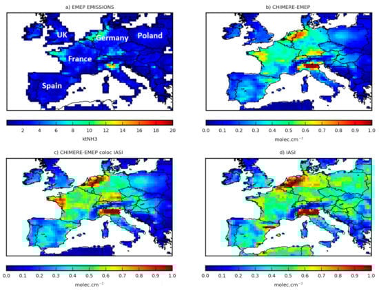
Figure 1.
(a) Mean EMEP NH3 emissions, in ktNH3, and mean average of (b) the simulated CHIMERE-EMEP NH3VCD, (c) the CHIMERE-EMEP-colocIASI NH3 VCD and (d) the IASI-v3R observations, over the continental domain, in molec.cm−2, for the period 2008–2015.
The chemical scheme used in CHIMERE is MELCHIOR-2, with more than 100 reactions [18], including 24 for inorganic chemistry. For inorganic species, aerosol thermodynamic equilibrium is achieved using the ISORROPIA model [34]. The parameterization of NH3 dry deposition is unidirectional in CHIMERE. However, Azouz et al. [35] assessed that such regional models usually operating with large grid cell sizes simulate the average NH3 dry deposition flux over a large domain of simulation quite well when comparing to a small-scale Gaussian model with unidirectional deposition.
Three sets of 8-year simulations, described in Table 1, have been performed to evaluate the impact of the meteorology and of NH3, NOx, and SOx European emission changes on the NH3 VCD trends. To this end, climatological values from the LMDZ-INCA global model [36] are used to prescribe the NH3, NO2, and SO2concentrations at the lateral and top boundaries. First, we have run reference simulations from 2008 to 2015, called “CHIMERE-EMEP” in the following. Then, we have performed sensitivity tests. We have run simulations with all the anthropogenic EMEP emissions kept constant at the 2008 levels, called “CHIMERE-EMEPconst” in the following. The objective of this sensitivity test is to assess the impact of the changes in meteorology on the NH3 VCD trend. We have also run simulations with only NOx and SOx anthropogenic EMEP emissions kept constant at the 2008 levels, called “CHIMERE-EMEPconstNS” in the following. The objective of this sensitivity test is to assess the impact of the changes in NOx and SOx emissions on the NH3 VCD trend.

Table 1.
Description of the CHIMERE simulations performed in this study.
2.2. IASI-v3R NH3 VCD
To quantify and understand the recent variability of NH3 over the 2008–2015 period, we use data from the IASI-A instrument, flying on a low sun-synchronous polar orbit since October 2006, with equator crossing times of 09:30 (descending mode) and 21:30 (ascending mode) LST [37]. The algorithm used to retrieve NH3 columns from the radiance spectra is described in Whitburn et al. [38], Van Damme et al. [39], and Franco et al. [40]. We use the ANNI-NH3-v3R-ERA5 dataset, called IASI-v3R in the following, which is relevant for inter-annual comparison and trend analyses [11]. It relies on ERA5 ECMWF meteorological input data [41].
The IASI total columns are averaged into “super-observations” (average of all IASI data within the 0.5° × 0.5° resolution and within the physical time step of CHIMERE). We have followed the recommendations formulated in Van Damme et al. [39] for post-filtering and for averaging data in time and space. We also only consider land measurements from the morning overpass. The analysis of the uncertainty distribution reveals uncertainties generally below 30% over source areas for the morning overpass time measurements. For regions with low NH3 columns in contrast, the uncertainty is typically larger than 150% [38]. We first consider the IASI-v3R data over the whole year (see Section 3). Nevertheless, there is a strongly lower number of super-observations during autumn and winter than in spring and summer (e.g., 41,526 super-observations in January against 77,400 in March 2015, Table 2). In addition, some studies have shown that the IASI observations are subject to large errors because of the lower spectral signal to noise ratio in autumn and in winter than in spring and summer [42,43]. As in these studies, we consequently also perform the analysis excluding the IASI-v3R data for autumn and winter.
Table 2.
Monthly number of IASI-v3R super-observations, in 2015.
2.3. Time Series Analysis Method
We calculate the gridded monthly budgets of NH3, NOx, and SOx EMEP emissions. We also compute gridded monthly averages of NH3, NO2, and SO2 VCDs simulated with CHIMERE over land. We compute the gridded monthly averages of NH3 IASI-v3R VCD, from daily gridded super-observations.
To derive the trends, we first calculate the monthly time series using these gridded monthly averages or monthly budgets at the CHIMERE resolution. National trends are calculated from monthly averages by taking into account the grid cells covered by each country only.
The monthly mean time series are used to calculate a mean 2008–2015 seasonal cycle. This cycle is then used to deseasonalize the monthly mean time series by calculating the anomalies. The linear trend is then calculated based on the monthly anomalies and a linear regression, as in Dufour et al. [44]. It is presented in percent per year in the following. As an ordinary linear regression is used for trend calculation, the trends uncertainties are calculated as the t test value multiplied with the standard error of the trends, which correspond to the 95 % confidence interval.
3. Results
3.1. Spatial Variability and Seasonal Cycles of Simulated and Observed NH3 VCD
Figure 1a presents the spatial variability of the annual EMEP NH3 emissions, showing strong hot-spots particularly over the Netherlands, the Po Valley and the French Brittany region, known as major European animal husbandry sources [23,33,45]. Figure 1b, presenting the average of NH3 VCDs simulated by CHIMERE over the period 2008-2015, shows similar patterns. When the CHIMERE-EMEP NH3 VCDs are collocated with the IASI-v3R observations (i.e., by considering the model only where and when IASI super-observations are available), the VCDs are called “CHIMERE-EMEP-colocIASI NH3 VCDs”. The simulated CHIMERE-EMEP-colocIASI NH3 VCD present different patterns with higher values over France and Germany than those of the CHIMERE-EMEP NH3 VCDs (Figure 1c). This indicates that the sampling linked to the IASI-v3R observations (i.e., morning overpass, cloud-free scenes) has a strong impact on the simulated NH3 VCD spatial patterns. Figure 1d presents the spatial variability of the average of the NH3 IASI-v3R super-observations over the entire period 2008–2015. Compared to these super-observations, the CHIMERE-EMEP-colocIASI simulation often under-estimates the NH3 VCDs (e.g., over Spain, over Eastern Europe). On the contrary, the simulated CHIMERE-EMEP-colocIASI NH3 VCDs are higher than IASI over northern France, particularly over the Bretagne region, and over southern Germany. This is probably due to a misrepresentation of livestock emissions. Bretagne in France [32] and Southern Germany are indeed regions known for their livestock activity.
The simulated CHIMERE-EMEP and CHIMERE-EMEP-colocIASI NH3 VCDs show a similar monthly variability (Figure 2). CHIMERE-EMEP, CHIMERE-EMEP-colocIASI and IASI-v3R, NH3 VCD also present similar seasonal cycles (Figure 2), the latter ones presenting a temporal correlation of 0.59 from 2008 to 2015. Maximums are seen in spring, when ammonia emissions are enhanced due to mineral fertilizer use in accordance with crop requirements [23,32,46,47,48], and a minimum in winter. However, it should be noted that IASI often shows a strong peak in summer in addition to the spring peak, whereas CHIMERE only shows a slight peak in summer some years (e.g., in 2009, in 2011). This result could point to a misrepresentation of the temporal profiles by GENEMIS, to missing emission sources during summertime, either due to more than expected fertilizer use in summertime or to increased volatilization from soils (not including in CHIMERE). Marais et al. [43], estimating the UK ammonia emission from satellite observations including IASI, consistently showed a summer peak associated with dairy cattle farming.
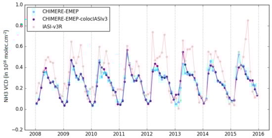
Figure 2.
Monthly means of NH3 VCD simulated by CHIMERE-EMEP (in cyan) and by CHIMERE-EMEP-colocIASI (in purple) and observed by IASI-v3R (in pink) over the continental domain, in molec.cm−2, from January 2008 to December 2015. Units are in 1016 molec.cm−2.
The spring peak simulated by CHIMERE occurs in April, due to the GENEMIS seasonal temporal profile used for the temporalization of emissions. These peaks sometimes present a gap of 1month compared to the IASI observations (e.g., peak in March 2012 and in March 2014 for IASI).
The amplitude of these seasonal cycles can also be different. IASI shows higher NH3 VCDs than CHIMERE mainly in spring and in summer, explaining a mean negative bias of CHIMERE compared to IASI of about −32% over the 2008–2015 period. These features can be probably explained by a misrepresentation of the amplitude of NH3 emissions in the bottom-up inventory [23,32], using a fixed and meteorology independent monthly emission profiles as mentioned previously.
3.2. Trends of Simulated and Observed NH3 VCDs
To answer the questions raised in the introduction about diverging trends in the NH3 emissions and observed NH3, we have analyzed the trendsin NH3 VCD simulated by the CHIMERE and we have performed sensitivity tests to assess the impact of meteorology, and of NH3, NOx, and SOx emissions on these trends. We have then confronted the simulated trends against the trends observed by the IASI satellite observations.
3.2.1. Disparities between the Trends in EMEP Ammonia Emissions Reported by Countries
According to the study of EEA [6], based on the EMEP emissions, NH3 emissions have seen no or only very small changes over Europe as a whole from 2008 to 2015. Nevertheless, as seen in Figure 3a, the trends in reported NH3 EMEP emissions from 2008 to 2015 exhibit strong disparities depending on the countries, with significant decreases especially over the Netherlands, Denmark, France, and Poland. On the contrary, significant increases are seen over other countries such as Germany, UK, and Spain. These disparities have also been noticed in the EDGAR-v5inventory [11].
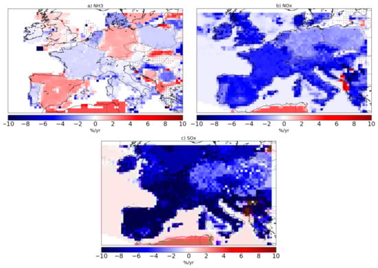
Figure 3.
Eight-year trends of (a) NH3, (b) NOx, and (c) SOx emissions in the EMEP inventory. Pixels with insignificant trend, with a p-value higher than 0.05, are shown with a cross symbol. Units are in%/yr.
Only few statistics are available to evaluate these reported trends. As livestock and spreading emissions strongly contribute to NH3 emissions, the trends in NH3 emissions could be partly due to the evolution of the bovine herd or to the evolution of the fertilizer consumption. Nevertheless, European statistics do not show a decrease in the bovine population in France, Germany, Poland, the Netherlands, and Spain for example, at least from 2011 to 2015 (data since 2008 are not available to our knowledge) [49]. It is, however, interesting to note that the fertilizer consumption has increased in France, Germany, Poland, Spain, and UK [50]. From 2008 to 2015, the fertilizer consumption has indeed increased from 152 to 170 kg per hectare of arable land in France, from 160 to 202 kg per hectare of arable land in Germany, from 158 to 174 kg per hectare of arable land in Poland, and from 106 to 151 kg per hectare of arable land in Spain. Over UK, the fertilizer consumption has strongly dropped from 2008 to 2009 (257 against 212 kg per hectare of arable land, respectively) and has then increased to 252 kg per hectare of arable land in 2015, due to increased use of urea-based fertilizers [51]. In the Netherlands, the fertilizer consumption seems to remain similar between 268 kg per hectare of arable land in 2008, and 267 in 2015 [50]. These statistics on the evolution of the bovine herd from EUROSTAT [49] and of the fertilizer consumption from World Bank [50] do not support our analysis of the geographic disparity for the NH3 emission trends in the EMEP bottom-up inventory. As these bottom-up inventories are based on countries reporting, the disparities can be explained by different procedures between countries to calculate and report the ammonia emissions [11]. This feature is one of the limitations from bottom-up inventories to estimate consistent long-term trends in NH3 emissions and consequently in NH3 VCDs.
3.2.2. Strong Increase of Simulated European NH3 VCDs
Over the continental domain, the CHIMERE-EMEP simulated NH3 VCDs show a significant positive trend of +2.7 ± 1.0%/yr (Table 3). At the national scale, the CHIMERE-EMEP VCD significantly positive trends over Spain, Germany, UK, France, and Poland are of about +4.9 ± 1.9%/yr, + 3.2 ± 1.6 %/yr, +2.7 ± 2.4%/yr, +2.4 ± 1.0%/yr, and +2.6 ± 2.2%/yr, respectively (Table 3). The CHIMERE-EMEP simulated NH3 VCDs indeed show significant positive trends over large parts of Spain, Germany, UK, and Poland (Figure 4a). Over large parts of France, Italy, and Eastern Europe, however, the CHIMERE-EMEP simulated NH3 VCDs show insignificant trends (Figure 4a).
Table 3.
Eight-year trends of NH3 VCD simulated by CHIMERE with the different sensitivity tests detailed in Section 2.1 and observed by IASI-V3R, for different European countries. The statistical method provides 2σ uncertainties of the trend values. Trends with a p-value equal or lower than 0.05, with change exceeding the uncertainty, are shown in bold. Units are in %/yr.
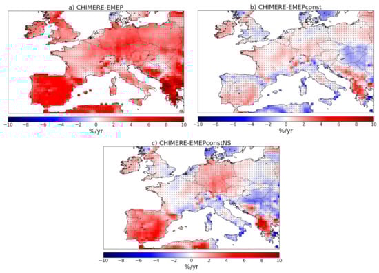
Figure 4.
Eight-year trends of NH3 VCD (a) with the CHIMERE-EMEP simulations, (b) simulated by CHIMERE with all anthropogenic EMEP emissions kept constant at the 2008 levels, and (c) simulated by CHIMERE with NOx and SOx anthropogenic EMEP emissions kept constant at the 2008 levels, over Europe for the period 2008–2015. Pixels with insignificant trend, with a p-value higher than 0.05, are shown with a cross symbol. Units are in %/yr.
3.2.3. Simulated NH3 VCD Increase Driven by NH3, SO2 and NOx Emissions
The NH3 VCD 8-year trends simulated by CHIMERE could be driven by meteorology and by trends in anthropogenic NH3, SOx, and NOx emissions. Different sensitivity tests have been performed to understand these trends. First, the CHIMERE-EMEPconst simulation is run with all anthropogenic EMEP emissions kept constant at the 2008 levels for the 2008–2015 period to assess the impact of the changes in meteorology on the NH3 VCD trend. The trends of the CHIMERE-EMEPconst simulated VCDs often become close to zero or slightly positive. These trends are considered as insignificant everywhere in Europe (except over parts of Albania and Greece, Figure 4b). This demonstrates that the impact of meteorology changes between 2008 and 2015 on NH3 VCD trends may be weak over Europe, as already shown for other parts of the world (by WichinkKruit et al., [15] for the Netherlands, by Yu et al. [16] for the United States, and by Lachatre et al. [17] for Eastern China).
The differences between the CHIMERE-EMEPconst and the CHIMERE-EMEPconstNS simulations—between Figure 4b,c—can only be explained by changes in NH3 emissions. When the variability of NH3 emissions is considered in the CHIMERE-EMEPconstNS simulation, the NH3 VCD trends become stronger and significantly positive over large parts of Spain and Germany (Figure 4c), consistently with the significant positive trends of their NH3 emissions in the EMEP inventory (Figure 3a). On the contrary, when the trends in NH3 emissions are significantly negative in the EMEP inventory (Figure 3a), the NH3 VCD trends mainly remain small and insignificant over large parts of Europe (e.g., over France, Italy, Poland, Figure 4c).
However, the evolution of NH3 emissions between 2008 and 2015 alone does not fully explain the strong and significantly positive simulated NH3 surface and VCD CHIMERE-EMEP trends over Europe. The strong difference in the trend estimates between the CHIMERE-EMEPconstNS (Figure 4c), with constant NOx and SOx emissions through the 2008–2015 period, and the CHIMERE-EMEP simulations (Figure 4a) demonstrate the strong impact of the decrease in NOx (Figure 3b) and SOx (Figure 3c) emissions estimated in the EMEP inventory on the NH3 surface and VCD trends. The most significant reaction of ammonia in the atmosphere is indeed its neutralization of acidic species–sulfuric acid H2SO4 and nitric acid HNO3, for which SO2 and NOx are precursors, respectively. This mainly determines the amount of ammonia that remains in the gas phase and the amount that becomes particulate NH4+. When NOx and SOx emissions are decreased, it leads to (i) a decrease in NO2 (Figure 5a) and SO2 concentrations (Figure 5b), and then to (ii) an increase in NH3 concentrations in the atmosphere. Our results are consistent with previous studies over the US and over Eastern China [16,17,52].
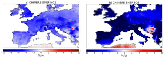
Figure 5.
Eight-year trends of (a) NO2VCD and (b) SO2VCD, simulated by CHIMERE with the set-up described in Section 2.1, for the period 2008–2015. Pixels with insignificant trend are shown with a cross symbol. Units are in %/yr.
3.2.4. Comparison of the Simulated NH3 VCD Trends to the IASI-v3R Satellite Observations
As for the spatial variability (Section 3.1), it is important to note that the sampling linked to the IASI-v3R observations (i.e., morning overpass, cloud-free scenes) has a strong impact on the simulated NH3 VCD trends. When the CHIMERE-EMEP VCDs are collocated with the IASI-v3R observations, the simulated CHIMERE-EMEP-colocIASI VCDs remain positive and significant over large parts of Spain, northeastern France, Germany, and Greece, but become mainly insignificant over Eastern Europe (Figure 6a). It is interesting to see that a lower number of pixels show a significant trend, even over Western Europe (e.g., in France or in Italy). This is probably due to the lower sampling frequency.
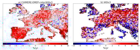
Figure 6.
Eight-year trends of NH3 VCD (a) simulated by CHIMERE with the set-up described in Section 2.1 and collocated with IASI-v3R observations, and (b) observed by IASI-v3R observations. Pixels with insignificant trend, with a p-value higher than 0.05, are shown with a cross symbol. Units are in%/yr.
The IASI-v3R observations show stronger positive trends over northern France, Germany, and Poland than for the simulated CHIMERE-EMEP-colocIASI VCDs, confirming their signs. However, the IASI-v3R observations present contradictory trends over Spain, southern France, Italy, and southeastern Europe.
In addition, the trends shown by the IASI-v3R observations are found insignificant almost everywhere in Europe (Figure 6b) and therefore complicate the comparison. This is not in agreement with Van Damme et al., [11], showing significant positive trends at the national scale for different European countries, but for a different period focusing on the evolution of the NH3 IASI VCDs between 2008 and 2018. Nevertheless, as recalled in the introduction, a non-negligible part of this2008–2018 increase in Europe seems to be mainly due to exceptionally warm and dry weather conditions in 2018, favoring the NH3 volatilization [11] and perhaps explaining the differences in terms of significance between the two studies.
The simulated NH3 VCD increase is confirmed by IASI-v3R satellite observations in spring and summer, whenammonia emissions strongly contribute to the annual budget in accordance with crop requirements and when NH3 VCDs are high (Figure 2). When analyzing the inter-annual seasonal variations (Figure 7), we can see that the disagreements between IASI and CHIMERE-EMEP-colocIASI VCD trends seem to be particularly due to the winter period. CHIMERE indeed shows a slight increase whereas IASI shows a strong decrease in the winter NH3 VCDs, by more than a factor of two (Figure 7). Nevertheless, the IASI observations are subject to large errors because of low spectral signal to noise ratio in winter and they are often removed from the analysis [32,42,43]. However, when the IASI super-observations of autumn and winter are excluded, both IASI and CHIMERE show an increase in NH3 VCDs from 2008 to 2015 (Figure 7). Over the entire domain, this significant increase is even higher with IASI (+2.9 ± 2.6 %/yr, Table 4) than with CHIMERE (+2.3 ± 1.4 %/yr, Table 4), due to higher IASI trends over Germany, Czech Republic, and Poland (Figure 8). At the national scale, CHIMERE-EMEP-colocIASI and IASI both show insignificant trends over France and UK, when taking into account spring and summer only (Table 4). They both show significant trends over Germany, with stronger trends estimated by IASI compared to CHIMERE-EMEP-colocIASI (Table 4). However, they still show divergences about significance over Spain: CHIMERE-EMEP-colocIASI estimates a strong significant increase in NH3 VCDs (+4.4 ± 2.2 %/yr, Table 4) while the IASI trend remains positive but insignificant. Over Poland, IASI estimates a strong significant increase in NH3 VCDs (+6.0 ± 3.9 %/yr, Table 4) while the CHIMERE-EMEP-colocIASI trend are also positive (+2.8 ± 3.0 %/yr, Table 4) but insignificant.
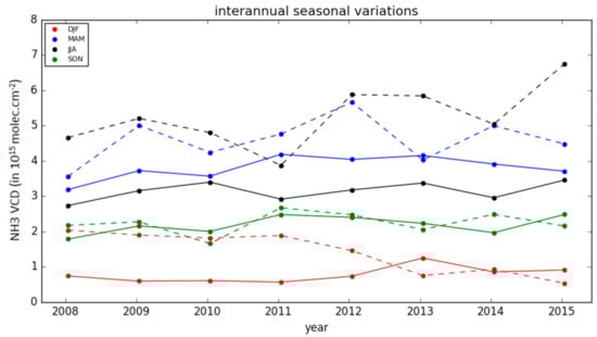
Figure 7.
Inter-annual seasonal variations of NH3 VCD, for the months of December, January, and February DJF in winter (in red), for the months of March, April, and May MAM in spring (in blue), for the months of June, July, and August JJA in summer (in black), for the months of September, October, and November SON in autumn (in green), from 2008 to 2015, in 1015molec.cm−2. Solid lines represent the simulated NH3 VCDs whereas the dotted lines represent the observed NH3 IASI VCDs.
Table 4.
Eight-year trends of NH3 VCD simulated by CHIMERE-EMEP-colocIASI and observed by IASI-V3R for different European countries, taking into account the months of March, April, and May MAM in spring and the months of June, July, and August JJA in summer only. Trends with a p-value equal or lower than 0.05 with change exceeding the uncertainty are shown in bold. Units are in %/yr.
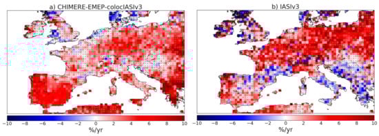
Figure 8.
Eight-year trends of NH3 VCD (a) simulated by CHIMERE-EMEP-colocIASI and (b) observed by IASI-v3R observation, taking into account the months of March, April, and May in spring and the months of June, July, and August in summer only. Pixels with insignificant trend, with a p-value higher than 0.05, are shown with a cross symbol. Units are in %/yr.
The remaining differences about the significance and magnitude between the simulated and observed trends can have several possible explanations. It may be due to a misrepresentation of the NH3 emission trends in the EMEP inventory. It may also be explained by a misrepresentation of the NOx and SOx emission trends in the EMEP inventory and consequently of the NO2 and SO2 simulated VCD trends. Indeed, the NO2 and SO2 VCDs observed by the Monitoring Ozone Instrument (OMI) between 2008 and 2015 do not show a decrease at the European scale in the study of Evangeliou et al. [53]. Over urban areas in Western Europe, satellite observations from OMI confirm the drop in the simulated CHIMERE NO2 tropospheric columns from 2008 to 2017 but OMI hardly show significant negative trends over Central and Eastern Europe urban areas and over rural areas [54]. In the framework of the EURODELTA multi-model experiment, the study of Ciarelli et al. [25] investigated the capability of the models to reproduce observed long-term air quality trends, at rural background EMEP stations, mainly located over Northern and Central Europe. With emissions estimated using the Greenhouse gas Air Pollution Interactions and Synergies (GAINS) model, they have shown that regional CTMs including CHIMERE tend to overestimate the fraction of significantly decreasing NO2 trend compared to 25 EMEP stations, for the period 2000-2010, while the SO2 trends seems to be better represented by CHIMERE. Finally, it can be due to a misrepresentation of the ammonia phase partitioning in the CHIMERE model, and warrant further investigation.
4. Conclusions
In this study, we have first analyzed the seasonal cycle in NH3 VCD simulated by the CHIMERE regional CTM from 2008 to 2015 and we have confronted this seasonality against the IASI satellite observations. CHIMERE and IASI present seasonal cycles with maximum in spring, and minimum in winter. The spring maximum simulated by CHIMERE, occurring in April due to the GENEMIS seasonal temporal profile used for the temporalization of emissions, sometimes presents a 1-month gap compared to the IASI observations. IASI often shows a strong peak in summer in addition to the spring peak, whereas CHIMERE only shows a slight peak in summer some years. This result could point to a misrepresentation of the temporal profile by GENEMIS, to missing emission sources during summertime (e.g., from dairy cattle farming as identified by Marais et al. [43] over UK), either due to more than expected fertilizer use or to increased volatilization under warmer conditions.
Then, we have analyzed the recent trends in NH3 VCDs simulated by the CHIMERE and we have performed sensitivity tests to assess the impact of meteorology, and of NH3, NOx, and SOx emissions on these trends. Over the entire European domain, the simulated NH3 VCDs show a significant positive trend of +2.7 ± 1.0%/yr. This simulated NH3 VCD increase at the European scale is confirmed by IASI-v3R satellite observations in spring and summer, whenammonia emissions strongly contribute to the annual budget in accordance with crop requirements. Nevertheless, there are remaining differences about the significance and magnitude between the simulated and observed trends at the national scale and it warrants further investigation.
Our simulations indicate that the simulated positive trends over Europeare mainly due to i) to the trends in NH3emissions and ii) to the negative trends in NOx and SOxemissions. The impact of reductions in NO2 and SO2 emissions on NH3 concentrations should therefore be taken into account in future policies. The quantification of these relative contributions would warrant further investigation. In addition,these conclusions are dependent to the accuracy of the reported NOx, SOx, and NH3 emissions by countries to EMEP/CEIP and their trends. For the development of efficient policies, the respective impact of NOx and SO2 emission trends on NH3 levels should be further investigated.As we have shown heterogeneous trends over Europe in the EMEP NH3 emissions with strong disparities depending on the country, the procedures to calculate and report ammonia emissions also warrant further investigation. This is critical for assessing reliability of European mitigation strategies for air quality.
Author Contributions
Conceptualization, A.F.-C.; methodology, A.F.-C. and G.D.; formal analysis, A.F.-C., G.D. and M.B.; investigation, A.F.-C. and G.D.; data curation, G.S., M.V.D., P.-F.C., L.C. and C.C.; writing—original draft preparation, A.F.-C., G.D., M.B., G.S., G.F., M.V.D., P.-F.C., L.C. and C.C.; writing—review and editing, A.F.-C., G.D. and M.B.; All authors have read and agreed to the published version of the manuscript.
Funding
This research received no external funding.
Institutional Review Board Statement
Not applicable.
Informed Consent Statement
Not applicable.
Data Availability Statement
The CHIMERE regional chemistry transport model [18,19] and its technical documentation can be found here: www.lmd.polytechnique.fr/chimere/ (accessed on 1 June 2019). The ANNI-NH3-v3.0R NH3 total columns [39] can be found here: https://iasi.aeris-data.fr/nh3/ (accessed on 1 June 2019).
Acknowledgments
This research has been supported by the Centre National d’Etudes Spatiales, CNES. The research in Belgium was funded by the Belgian Science Policy Office (BELSPO) (Prodex HIRS and FED-tWIN ARENBERG) and the Air Liquide Foundation (TAPIR project). L. Clarisse is Research Associate supported by the Belgian F.R.S.-FNRS. This work was granted access to the HPC resources of TGCC under the allocation A0070107232 and A0080107232. IASI is a joint mission of EUMETSAT and the Centre National d’Etudes Spatiales (CNES, France). The authors acknowledge the AERIS data infrastructure for providing access to the IASI data in this study and ULB-LATMOS for the development of the retrieval algorithms.
Conflicts of Interest
The authors declare no conflict of interest.
References
- Erisman, J.W.; Bleeker, A.; Galloway, J.; Sutton, M.S. Reduced nitrogen in ecology and the environment. Environ. Pollut. 2007, 150, 140–149. [Google Scholar] [CrossRef] [Green Version]
- EEA European Environment Agency: Effects of Air Pollution on European Ecosystems-Past and Future Exposure of European Freshwater and Terrestrial Habitats to Acidifying and Eutrophying Air Pollutants; Technical Report. 2014. Available online: https://www.eea.europa.eu/publications/effects-of-air-pollution-on (accessed on 1 June 2021).
- Lelieveld, J.; Evans, J.S.; Fnais, M.; Giannadaki, D.; Pozzer, A. The contribution of outdoor air pollution sources to premature mortality on a global scale. Nature 2015, 525, 367–371. [Google Scholar] [CrossRef] [PubMed]
- Directive (EU) 2001/81/EC of the European Parliament and of the Council of 23 October 2001 on National Emission Ceilings for Certain Atmospheric Pollutants. 2001. Available online: https://eur-lex.europa.eu/eli/dir/2001/81/oj (accessed on 1 September 2021).
- Directive (EU) 2016/2284 of the European Parliament and of the Council of 14 December 2016 on the Reduction of National Emissions of Certain Atmospheric Pollutants, Amending Directive 2003/35/EC and Repealing Directive 2001/81/EC. 2016. Available online: http://data.europa.eu/eli/dir/2016/2284/oj (accessed on 1 September 2021).
- EEA European Environment Agency: Air Quality in Europe—2020 Report. 2020. Available online: https://www.eea.europa.eu/publications/air-quality-in-europe-2020-report (accessed on 1 September 2021).
- Von Bobrutzki, K.; Braban, C.F.; Famulari, D.; Jones, S.K.; Blackall, T.; Smith, T.E.L.; Blom, M.; Coe, H.; Gallagher, M.; Ghalaieny, M.; et al. Field inter-comparison of eleven atmospheric ammonia measurement techniques. Atmos. Meas. Technol. 2010, 3, 91–112. [Google Scholar] [CrossRef] [Green Version]
- Hertel, O.; Skjøth, C.A.; Reis, S.; Bleeker, A.; Harrison, R.M.; Cape, J.N.; Fowler, D.; Skiba, U.; Simpson, D.; Jickells, T.; et al. Governing processes for reactive nitrogen compounds in the European atmosphere. Biogeosciences 2012, 9, 4921–4954. [Google Scholar] [CrossRef] [Green Version]
- Flechard, C.R.; Nemitz, E.; Smith, R.I.; Fowler, D.; Vermeulen, A.T.; Bleeker, A.; Erisman, J.W.; Simpson, D.; Zhang, L.; Tang, Y.S.; et al. Dry deposition of reactive nitrogen to European ecosystems: A comparison of inferential models across the NitroEurope network. Atmos. Chem. Phys. 2011, 11, 2703–2728. [Google Scholar] [CrossRef] [Green Version]
- Warner, J.X.; Dickerson, R.R.; Wei, Z.; Strow, L.L.; Wang, Y.; Liang, Q. Increased atmospheric ammonia over the world’s major agricultural areas detected from space. Geophys. Res. Lett. 2017, 44, 2875–2884. [Google Scholar] [CrossRef]
- Van Damme, M.; Clarisse, L.; Franco, B.; A Sutton, M.; Erisman, J.W.; Kruit, R.W.; van Zanten, M.; Whitburn, S.; Hadji-Lazaro, J.; Hurtmans, D.; et al. Global, regional and national trends of atmospheric ammonia derived from a decadal (2008–2018) satellite record. Environ. Res. Lett. 2021, 16, 055017. [Google Scholar] [CrossRef]
- Clarisse, L.; Shephard, M.; Dentener, F.; Hurtmans, D.; Cady-Pereira, K.; Karagulian, F.; Van Damme, M.; Clerbaux, C.; Coheur, P.-F. Satellitemonitoringofammonia:Acasestudyof the San Joaquin Valley. J. Geophys. Res. 2010, 115, D13302. [Google Scholar] [CrossRef] [Green Version]
- Clarisse, L.; Clerbaux, C.; Dentener, F.; Hurtmans, D.; Coheur, P. Global ammonia distribution derived from infrared satellite observations. Nat. Geosci. 2009, 2, 479–483. [Google Scholar] [CrossRef]
- Sutton, M.A.; Asman, W.A.H.; Ellermann, T.; Van Jaarsveld, J.A.; Acker, K.; Aneja, V.; Duyzer, J.; Horvath, L.; Paramonov, S.; Mitosinkova, M.; et al. Establishing the Link between Ammonia Emission Control and Measurements of Reduced Nitrogen Concentrations and Deposition. Environ Monit Assess 2003, 82, 149–185. [Google Scholar] [CrossRef]
- WichinkKruit, R.J.; Aben, J.; de Vries, W.; Sauter, F.; van der Swaluw, E.; van Zanten, M.C.; van Pul, W.A.J. Modelling trends in ammonia in the Netherlands over the period 1990–2014. Atmos. Environ. 2017, 154, 20–30. [Google Scholar] [CrossRef]
- Yu, F.; Nair, A.A.; Luo, G. Long-term trend of gaseous ammonia over the United States: Modeling and comparison with observations. J. Geophys. Res. Atmos. 2018, 123, 8315–8325. [Google Scholar] [CrossRef] [PubMed] [Green Version]
- Lachatre, M.; Fortems-Cheiney, A.; Foret, G.; Siour, G.; Dufour, G.; Clarisse, L.; Clerbaux, C.; Coheur, P.-F.; Van Damme, M.; Beekmann, M. The unintended consequence of SO2 and NO2 regulations over China: Increase of ammonia levels and impact on PM2.5 concentrations. Atmos. Chem. Phys. 2019, 19, 6701–6716. [Google Scholar] [CrossRef] [Green Version]
- Menut, L.; Bessagnet, B.; Khvorostyanov, D.; Beekmann, M.; Blond, N.; Colette, A.; Coll, I.; Curci, G.; Foret, G.; Hodzic, A.; et al. CHIMERE 2013: A model for regional atmospheric composition modelling. Geosci. Model Dev. 2013, 6, 981–1028. [Google Scholar] [CrossRef] [Green Version]
- Mailler, S.; Menut, L.; Khvorostyanov, D.; Valari, M.; Couvidat, F.; Siour, G.; Turquety, S.; Briant, R.; Tuccella, P.; Bessagnet, B.; et al. CHIMERE-2017: From urban to hemispheric chemistry-transport modeling. Geosci. Model Dev. 2017, 10, 2397–2423. [Google Scholar] [CrossRef] [Green Version]
- Menut, L.; Bessagnet, B.; Briant, R.; Cholakian, A.; Couvidat, F.; Mailler, S.; Pennel, R.; Siour, G.; Tuccella, P.; Turquety, S.; et al. The CHIMERE v2020r1 online chemistry-transport model. Geosci. Model Dev. 2021, 14, 6781–6811. [Google Scholar] [CrossRef]
- Marécal, V.; Peuch, V.-H.; Andersson, C.; Andersson, S.; Arteta, J.; Beekmann, M.; Benedictow, A.; Bergström, R.; Bessagnet, B.; Cansado, A.; et al. A regional air quality forecasting system over Europe: The MACC-II daily ensemble production. Geosci. Model Dev. 2015, 8, 2777–2813. [Google Scholar] [CrossRef] [Green Version]
- Terrenoire, E.; Bessagnet, B.; Rouïl, L.; Tognet, F.; Pirovano, G.; Létinois, L.; Beauchamp, M.; Colette, A.; Thunis, P.; Amann, M.; et al. High-resolution air quality simulation over Europe with the chemistry transport model CHIMERE. Geosci. Model Dev. 2015, 8, 21–42. [Google Scholar] [CrossRef] [Green Version]
- Fortems-Cheiney, A.; Dufour, G.; Hamaoui-Laguel, L.; Foret, G.; Siour, G.; Van Damme, M.; Meleux, F.; Coheur, P.-F.; Clerbaux, C.; Clarisse, L.; et al. Unaccounted variability in NH3 agricultural sources detected by IASI contributing to European spring haze episode. Geophys. Res. Lett. 2016, 43, 5475–5482. [Google Scholar] [CrossRef] [Green Version]
- Cholakian, A.; Beekmann, M.; Coll, I.; Ciarelli, G.; Colette, A. Biogenic secondary organic aerosol sensitivity to organic aerosol simulation schemes in climate projections. Atmos. Chem. Phys. 2019, 19, 13209–13226. [Google Scholar] [CrossRef] [Green Version]
- Ciarelli, G.; Theobald, M.R.; Vivanco, M.G.; Beekmann, M.; Aas, W.; Andersson, C.; Bergström, R.; Manders-Groot, A.; Couvidat, F.; Mircea, M.; et al. Trends of inorganic and organic aerosols and precursor gases in Europe: Insights from the EURODELTA multi-model experiment over the 1990–2010 period. Geosci. Model Dev. 2019, 12, 4923–4954. [Google Scholar] [CrossRef] [Green Version]
- Menut, L.; Bessanet, B.; Siour, G.; Mailler, S.; Pennel, R.; Cholakian, A. Impact of lockdown measures to combat COVID-19 on air quality over western Europe. Sci. Total Environ. 2020, 741, 140426. [Google Scholar] [CrossRef] [PubMed]
- Owens, R.G.; Hewson, T. ECMWF Forecast User Guide, Reading. 2018. Available online: https://software.ecmwf.int/wiki/display/FUG/Forecast+User+Guide (accessed on 1 September 2019).
- Guenther, A.; Karl, T.; Harley, P.; Wiedinmyer, C.; Palmer, P.I.; Geron, C. Estimates of global terrestrial isoprene emissions using MEGAN (Model of Emissions of Gases and Aerosols from Nature). Atmos. Chem. Phys. 2006, 6, 3181–3210. [Google Scholar] [CrossRef] [Green Version]
- Vestreng, V.; Breivik, K.; Adams, M.; Wagner, A.; Goodwin, J.; Rozovskaya, O.; Oacyna, J. Inventory Review 2005-Emission Data Reported to CLRTAP and under the NEC Direc-Tive-Initial Review for HMs and POPs. In EMEP Status report; Norwegian Meteorological Institute: Oslo, Norway, 2005. [Google Scholar]
- Ebel, A.; Friedrich, R.; Rodhe, H. (Eds.) Tropospheric Modelling and Emission Estimation. Transport and Chemical Transformation of Pollutants in the Troposphere, chap. In GENEMIS: Assessment, Improvement, and Temporal and Spatial Disaggregation of European Emission Data; Springer: Berlin, Germany, 1997. [Google Scholar]
- Couvidat, F.; Bessagnet, B.; Garcia-Vivanco, M.; Real, E.; Menut, L.; Colette, A. Development of an inorganic and organic aerosol model (CHIMERE 2017β v1.0): Seasonal and spatial evaluation over Europe. Geosci. Model Dev. 2018, 11, 165–194. [Google Scholar] [CrossRef] [Green Version]
- Fortems-Cheiney, A.; Dufour, G.; Dufossé, K.; Couvidat, F.; Gilliot, J.-M.; Siour, G.; Beekmann, M.; Foret, G.; Meleux, F.; Clarisse, L.; et al. Do alternative inventories converge on the spatiotemporal representation of spring ammonia emissions in France? Atmos. Chem. Phys. 2020, 20, 13481–13495. [Google Scholar] [CrossRef]
- Hamaoui-Laguel, L.; Meleux, F.; Beekmann, M.; Bessagnet, B.; Genermont, S.; Cellier, P.; Letinois, L. Improving ammonia emissions in air quality modelling for France. Atmos. Environ. 2014, 92, 584–595. [Google Scholar] [CrossRef]
- Nenes, A.; Pandis, S.N.; Pilinis, C. ISORROPIA: A new thermodynamic equilibrium model for multiphase multicomponent inorganic aerosols. Aquat. Geochem. 1998, 4, 123–152. [Google Scholar] [CrossRef]
- Azouz, N. Comparison of spatial patterns of ammonia concentration and dry deposition flux between a regional Eulerian chemistry-transport model and a local Gaussian plume model. Air Qual. Atmos. Health 2019, 12, 719–729. [Google Scholar] [CrossRef]
- Szopa, S.; Foret, G.; Menut, L.; Cozic, A. Impact of large-scale circulation on European summer surface ozone: Consequences for modeling. Atmos. Environ. 2008, 43, 1189–1195. [Google Scholar] [CrossRef]
- Clerbaux, C.; Boynard, A.; Clarisse, L.; George, M.; Hadji-Lazaro, J.; Herbin, H.; Hurtmans, D.; Pommier, M.; Razavi, A.; Turquety, S.; et al. Monitoring of atmospheric composition using the thermal infrared IASI/MetOp sounder. Atmos. Chem. Phys. 2009, 9, 6041–6054. [Google Scholar] [CrossRef] [Green Version]
- Whitburn, S.; Van Damme, M.; Clarisse, L.; Bauduin, S.; Heald, C.L.; Hadji-Lazaro, J.; Hurtmans, D.; Zondlo, M.A.; Clerbaux, C.; Coheur, P.-F. A flexible and robust neural network IASI-NH3 retrieval algorithm. J. Geophys. Res. Atmos. 2016, 121, 6581–6599. [Google Scholar] [CrossRef]
- Van Damme, M.; Whitburn, S.; Clarisse, L.; Clerbaux, C.; Hurtmans, D.; Coheur, P.-F. Version 2 of the IASI NH3 neural network retrieval algorithm: Near-real-time and reanalysed datasets. Atmos. Meas. Technol. 2017, 10, 4905–4914. [Google Scholar] [CrossRef] [Green Version]
- Franco, B.; Clarisse, L.; Stavrakou, T.; Müller, J.F.; Van Damme, M.; Whitburn, S.; Hadji-Lazaro, J.; Hurtmans, D.; Taraborrelli, D.; Clerbaux, C.; et al. A general framework for global retrievals of trace gases from IASI: Application to methanol, formic acid, and PAN. J. Geophys. Res. Atmos. 2018, 123, 13963–13984. [Google Scholar] [CrossRef] [Green Version]
- Hersbach, H.; Bell, B.; Berrisford, P.; Hirahara, S.; Horányi, A.; Muñoz-Sabater, J.; Nicolas, J.; Peubey, C.; Radu, R.; Schepers, D.; et al. The ERA5 global reanalysis. Q J R Meteorol. Soc. 2020, 146, 1999–2049. [Google Scholar] [CrossRef]
- Viatte, C.; Wang, T.; Van Damme, M.; Dammers, E.; Meleux, F.; Clarisse, L.; Shephard, M.W.; Whitburn, S.; Coheur, P.F.; Cady-Pereira, K.E.; et al. Atmospheric ammonia variability and link with particulate matter formation: A case study over the Paris area. Atmos. Chem. Phys. 2020, 20, 577–596. [Google Scholar] [CrossRef] [Green Version]
- Marais, E.A.; Pandey, A.K.; Van Damme, M.; Clarisse, L.; Coheur, P.F.; Shephard, M.W.; Cady-Pereira, K.E.; Misselbrook, T.; Zhu, L.; Luo, G.; et al. UK ammonia emissions estimated with satellite observations and GEOS-Chem. J. Geophys. Res. Atmos. 2021, 126, e2021JD035237. [Google Scholar] [CrossRef]
- Dufour, G.; Hauglustaine, D.; Zhang, Y.; Eremenko, M.; Cohen, Y.; Gaudel, A.; Siour, G.; Lachatre, M.; Bense, A.; Bessagnet, B.; et al. Recent ozone trends in the Chinese free troposphere: Role of the local emission reductions and meteorology. Atmos. Chem. Phys. 2021, 21, 16001–16025. [Google Scholar] [CrossRef]
- Van Damme, M.; Clarisse, L.; Heald, C.L.; Hurtmans, D.; Ngadi, Y.; Clerbaux, C.; Dolman, A.J.; Erisman, J.W.; Coheur, P.F. Global distributions, time series and error characterization of atmospheric ammonia (NH3) from IASI satellite observations. Atmos. Chem. Phys. 2014, 14, 2905–2922. [Google Scholar] [CrossRef] [Green Version]
- Skjøth, C.A.; Hertel, O.; Gyldenkærne, S.; Ellerman, T. Implementing a dynamical ammonia emission parameterization in thelarge-scale air pollution model ACDEP. J. Geophys. Res. 2004, 109, D06306. [Google Scholar] [CrossRef]
- Ramanantenasoa, M.M.J.; Gilliot, J.-M.; Mignolet, C.; Bedos, C.; Mathias, E.; Eglin, T.; Makowski, D.; Génermont, S. A new framework to estimate spatio-temporal ammonia emissions due to nitrogen fertilization in France. Sci. Total Environ. 2018, 645, 205–219. [Google Scholar] [CrossRef]
- Génermont, S.; Ramanantenasoa, M.M.J.; Dufossé, K.; Maury, O.; Mignolet, C.; Gilliot, J.-M. Data on spatio-temporal representation of mineral N fertilization and manure N application as well as ammonia volatilization in French regions for the crop year 2005/06. Data Brief 2018, 21, 1119–1124. [Google Scholar] [CrossRef] [PubMed]
- EUROSTAT. Bovine Population. Available online: https://ec.europa.eu/eurostat/databrowser/view/apro_mt_lscatl/default/table?lang=en (accessed on 1 June 2021).
- World Bank. Available online: https://data.worldbank.org/indicator/AG.CON.FERT.ZS?view=chart (accessed on 1 June 2021).
- Ricardo. UK Informative Inventory Report (1990 to 2018). 2020. Available online: https://uk-air.defra.gov.uk/assets/documents/reports/cat07/2003131327_GB_IIR_2020_v1.0.pdf (accessed on 1 June 2021).
- Schiferl, L.D.; Heald, C.L.; Van Damme, M.; Clarisse, L.; Clerbaux, C.; Coheur, P.-F.; Nowak, J.B.; Neuman, J.A.; Herndon, S.C.; Roscioli, J.R.; et al. Interannual variability of ammonia concentrations over the United States: Sources and implications. Atmos. Chem. Phys. 2016, 16, 12305–12328. [Google Scholar] [CrossRef] [Green Version]
- Evangeliou, N.; Balkanski, Y.; Eckhardt, S.; Cozic, A.; Van Damme, M.; Coheur, P.F.; Clarisse, L.; Shephard, M.W.; Cady-Pereira, K.E.; Hauglustaine, D. 10-year satellite-constrained fluxes of ammonia improve performance of chemistry transport models. Atmos. Chem. Phys. 2021, 21, 4431–4451. [Google Scholar] [CrossRef]
- Fortems-Cheiney, A.; Broquet, G.; Pison, I.; Saunois, M.; Potier, E.; Berchet, A.; Dufour, G.; Siour, G.; Denier van der Gon, H.; Dellaert, S.N.C.; et al. Analysis of the anthropogenic and biogenic NOx emissions over 2008–2017: Assessment of the trends in the 30 most populated urban areas in Europe. Geophys. Res. Lett. 2021, 48, e2020GL092206. [Google Scholar] [CrossRef]
Publisher’s Note: MDPI stays neutral with regard to jurisdictional claims in published maps and institutional affiliations. |
© 2022 by the authors. Licensee MDPI, Basel, Switzerland. This article is an open access article distributed under the terms and conditions of the Creative Commons Attribution (CC BY) license (https://creativecommons.org/licenses/by/4.0/).