Predictive Analysis of In-Vehicle Air Quality Monitoring System Using Deep Learning Technique

Abstract

In-vehicle air quality monitoring systems have been seen as promising paradigms for monitoring drivers’ conditions while they are driving. This is because some in-vehicle cabins contain pollutants that can cause drowsiness and fatigue to drivers. However, designing an efficient system that can predict in-vehicle air quality has challenges, due to the continuous variation in parameters in cabin environments. This paper presents a new approach, using deep learning techniques that can deal with the varying parameters inside the vehicle environment. In this case, two deep learning models, namely Long-short Term Memory (LSTM) and Gated Recurrent Unit (GRU) are applied to classify and predict the air quality using time-series data collected from the built-in sensor hardware. Both are compared with conventional methods of machine learning models, including Support Vector Regression (SVR) and Multi-layer Perceptron (MLP). The results show that GRU has an excellent prediction performance with the highest coefficient of determination value (R²) of 0.97.

1. Introduction

According to the World Health Organization (WHO), approximately 1.35 million fatal accidents have occurred around the world, and the number is increasing annually [1]. Within this number, the study states that 15% of these accidents are caused by driver drowsiness and impaired cognition ability. Moreover, agencies such as the American Automobile Association (AAA) predict that one out of eight accidents in the United States which require hospitalization happen because of driver drowsiness and fatigue [2]. Thus, this condition can be seen as a life-threatening event, especially when the driver is cruising at a high speed, and the damage caused by these accidents is even more severe to public lives and property.

Drowsiness can be caused by many factors. Among them are chronic driver fatigue, lack of sleep, and increased CO₂ concentration in the vehicle [3]. Some studies show that the cabin inside a vehicle contains different pollutants that can affect human health such as carbon monoxide (CO), carbon dioxide (CO₂), nitrogen dioxide (NO₂) and volatile organic compounds (VOC) [4,5]. They can cause various health concerns including impaired vision and physical coordination while driving, as well as dizziness and fatigue to the occupants [6]. Furthermore, these combinations make it difficult for drivers to operate vehicles on the road [7,8].

Over time, a new generation of vehicle manufacturers have concentrated on Heating, Ventilation and Air Conditioning (HVAC) systems to provide a fresh air mode or re-circulation (RC) mode options for the occupants. Most HVAC systems use RC modes to help in reducing the distribution of pollutants and gases which come from the exhaust system. However, since most of the major air pollutants cannot be seen with human eyes, drivers are not aware of the air quality inside the vehicle cabin. Nevertheless, they inhale oxygen and then replace it with carbon dioxide (CO₂), which acts as a part of contamination known as human bio-effluents [9]. The elevated concentration of CO₂ reduces individuals’ cognitive ability, which results in drowsiness, dizziness and fatigue [10].

Thus, there is a need to provide monitoring systems that can measure in-vehicle air pollutants and ultimately monitor drivers’ conditions while driving. Previous studies used monitoring technologies such as cameras and in-vehicle sensors that are difficult to install and may constrain the driver’s behavior. Most of the existing systems have employed artificial intelligence techniques to provide decision-making processes on air quality [11]. Such approaches include rule-based systems. Although they have made significant contributions in this area, real-time monitoring systems are still immature and remain challenging. This may be due to the need to provide various rules in order to allow the system to work efficiently. Detection accuracy also depends on the parameters inside the in-vehicle environment, which always vary continuously. Furthermore, these studies only focused on classifying the air quality in real-time, without having the ability to predict future conditions [12].

In order to provide accurate prediction tasks, real-time information on various pollutants in the vehicle is required. Up to this date, the information has not been available in an online and public repository, nor in a constantly updated database. There are only a few published works which focus on driver drowsiness and its relationship with air pollutants inside the vehicle. Furthermore, there is little information on the available systems on the market that can classify and predict the future state of in-vehicle conditions and visualize them in an interactive visualization mode.

This paper recognizes the above-mentioned limitations and addresses them by proposing a new approach to classify in-vehicle air quality and predict the future state of its conditions. In this respect, two deep learning models are used to handle the time-series data, which are Long Short-term Memory (LSTM) and Gated Recurrent Units (GRU). These methods are then compared with the conventional approaches of machine learning algorithms such as Support Vector Regression (SVR) and Multi-Layer Perceptron (MLP) to evaluate their performances in terms of performance metrics such as Root Mean Square Error (RMSE), Mean Absolute Error (MAE) and coefficient of determination (R²).

The remainder of the paper is organized as follows: Section 2 describes the previous work related to this study. Section 3 gives detailed explanations of the data used and the methodology applied to predict the future state. Section 4 presents the experimental results. Finally, Section 5 concludes the study and provides directions for future research.

2. Related Work

Studies in indoor air quality prediction have increased considerably in recent years. However, most of the main topics have focused on indoor or outdoor environments. It can be seen that most air quality indexes and standards are introduced for outdoors in the selected environment. Up to this date, air quality inside the vehicle cabin has not been included in any standards [13]. Over time, driver monitoring systems have been developed to monitor and measure drivers’ conditions while they are driving [14]. This is due to the progression in autonomous driving technologies, which promote precision driver safety and health [15]. One of the concerns in the driver monitoring system is drowsiness, a condition due to lack of oxygen and increase of air pollutants from the outside environment, such as CO, CO₂, and NO₂ [16]. Furthermore, air pollution is also a major concern that can affect drivers’ ability to focus on the road [17]. Studies show that long-term exposure to air pollution puts a high risk on human health, and results in respiratory and cardiovascular problems, neuropsychiatric complications, skin diseases and chronic illnesses such as cancer [18].

Several studies found that a high concentration of CO₂ could affect human decision-making performance. Although not immediately life-threatening, it had a significant impact, particularly when driving. Ref. [19] reported that seven out of nine cognitive function domains could be affected by the increase of CO₂ concentration in the vehicle cabin. Prolonged exposure to a high concentration of CO₂ (1400 ppm) affected human cognitive performance significantly, compared with 100% outdoor air ventilation and a moderate CO₂ (~945 ppm) condition. Meanwhile, ref. [20] conducted an experiment by collecting CO₂ concentrations every 5 min with two different air circulation modes. It found that the CO₂ concentration reached 3200 ppm after one hour and human subjects reported an unpleasant sensation occurring after 25 min. Table 1 presents the rest of the related work focusing on in-vehicle air quality systems.

Table 1. Related Work on In-vehicle Air Quality System.

Authors	Aim	Analysis Methods	Comments
[13]	Study the air quality inside the vehicle cabin during driving and engine idling.	T-test and Pearson Correlation model	The authors measured the in-vehicle air quality during driving and engine idling. They do not clearly state the difference between the driving and idling data. However, they found that CO2 and VOC gases exceeded the recommendation value of the Hong Kong Environmental Protection Department (HKEPD) AQI guidelines.
[21]	Use a fractional air recirculation system to improve the in-vehicle air quality	Mathematical model	The authors investigated the ideal ratio based on the open windows condition to measure the accumulation of CO2 and reduction of particle concentration. They state that the ideal CO2 concentration is from 1500 ppm to 2500 ppm.
[22]	Test self-pollution inside cabin vehicle	Mathematical model	The authors found a high occurrence of in-vehicle self-pollution in the test set. PM2.5 contributed a lot to the in-cabin exposure. The data logging used a laptop as the database. The study lacked real-time cloud-based monitoring.
[23]	Apply mobile sensing system to study the air quality inside the vehicle cabin	Time-based presentation	The authors presented the work by using the local database using a smartphone to record and show the level of air quality inside the vehicle cabin. Data collection using several vehicles showed that the system had worked successfully.
[24]	Visualize environmental air quality using software ExpoLIS	Linear regression	The work utilized installed sensors on vehicles to measure air quality of the drivers’ environment. All the collected data were analyzed using ExpoLIS and visualized using a web-based display.
[25]	Characterize air quality and thermal profile for electric vehicle cabin	Time-based data series	The presented work used particulate matter and VOC as the main parameters. The results compared recirculation and fresh air modes in the electric car cabin.

Air Quality Index (AQI) is used as a standard to measure the current air quality in the surrounding environments. In particular, it measures the state of each air quality parameter relative to human need or purposes [26]. This helps to show the public the current air quality and determine whether it has an impact on their health. Several AQIs have been established in different countries with different names, limit ranges and observation parameters. For example, the Air Quality Health Index (AQHI) has been introduced in Canada and Hong Kong [27]. Singapore utilizes the Pollutant Standard Index (PSI) while Malaysia uses the Air Pollution Index (API).

Several techniques have been introduced to predict air quality in the in-vehicle environment. Some use electronic devices that are attached to the driver’s skin to measure biological signals such as electrocardiography, electrooculography and electromyography [28]. They monitor variations in the brain signal and determine cognitive ability and psychological state for driving. Another approach involves the use of cameras, where visual information is obtained on the driver’s behavior [29]. Visual characteristics including the eyes and mouth are analyzed to detect signs of drowsiness or distraction such as yawning and eye activity. In recent years, new technology involving multi-modal sensors that can analyze drivers’ bio-signals has been emerging [30]. This includes the concentration of air pollutants in the car as well as particulate matter. The method is very convincing, as these gases can affect decision-making ability and information usage. Table 2 represents examples of pollutant gases that can affect a driver’s ability to drive properly in the in-vehicle cabin.

Table 2. Common Air Pollutants Found in In-vehicle cabin [31,32,33].

Air Pollutant	Health Effect
Carbon Dioxide (CO2)	Fatigue, drowsiness, headaches, dizziness, restlessness, a tingling or pins and needles feeling, difficulty breathing, sweating, tiredness, increased heart rate, elevated blood pressure, coma, asphyxia and convulsions.
Carbon Monoxide (CO)	Headache, fatigue, dizziness, drowsiness, nausea, confusion, and collapse, in addition to loss of consciousness and muscle weakness.
Ozone (O3)	Chest pain, coughing, throat irritation and congestion or worsening bronchitis, emphysema and asthma.
Particulate Matter (PM)	Premature death in people with heart and lung diseases. Aggravated asthma, decreased lung function and increased respiratory symptoms such as coughing and difficulty breathing.
Temperature	Heat cramps, heat exhaustion, heatstroke and hyperthermia.
Humidity	Excessive sweating, increased rate and depth of blood circulation and increased respiration.

With respect to the prediction system, artificial intelligence approaches have been widely used. Other traditional prediction methods use statistical techniques and mathematical models such as linear regression, principal component analysis (PCA) and multiple linear regression [34]. In addition, machine learning approaches such as Support Vector Machine (SVM) and Decision Tree (DT) are also used to classify air quality [30]. However, traditional prediction techniques are ill-suited for time-series applications, and prediction results always depend on the historical data [35]. Furthermore, features have to be selected and manually handcrafted each time the environment changes. This contributes to time-consuming and ineffective classification systems [36].

In recent years, studies have shown that deep learning models have an excellent capability of dealing with time-series data as well as with long-term dependencies of air quality prediction data. In particular, deep learning has gained increasing interest in the prediction field. The model contains hidden layers that have the capability of learning data patterns autonomously [37]. Furthermore, deep learning has advantages compared with other traditional approaches. These include the ability to extract features automatically without having to undergo handcrafted feature extraction. Moreover, deep learning utilizes the use of shallow features which are difficult to use with traditional methods. With respect to this study, researchers have applied a deep learning model to predict air quality. For example, ref. [38] applied an LSTM and Deep Autoencoder model to predict air quality in Seoul, South Korea. The study showed high prediction results using parameters such as PM₁₀ and PM_2.5. Moreover, ref. [39] also used particulate matter as the main parameter. The study applied LSTM and GRU models to predict air quality, and found that GRU had the highest performance rates compared to the LSTM model. Most of the studies only focused on indoor or outdoor air quality. In addition, the learning models were performed post-analysis, rather than in real-time systems.

From the review, it can be seen that most of the presented work focused on air quality prediction for indoor or outside environments. This paper has a different viewpoint, from which it investigates the capability of deep learning algorithms to predict air quality inside the vehicle cabin. The work compares the performance of deep learning with traditional machine learning algorithms using several parameters such as CO₂, particulate matter, temperature and humidity. This is important to ensure the safety of driver and passengers when driving vehicles on the road.

3. Proposed Method

3.1. Overall System Design

An integrated in-vehicle air quality monitoring system was developed for this study. The system is composed of multi-modal sensors that are integrated together to monitor gasses components in the vehicle cabin. Figure 1 presents the overall system architecture. It consists of three main sensors and one communication module. These sensors are used to monitor several parameters, including CO₂, PM_2.5 and PM₁₀, temperature and humidity. In addition, the SIM808 GSM communication module is used to provide the speed and location of the vehicle.

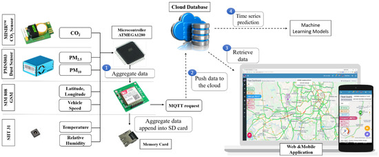
Figure 1. Overall System Design for Air Quality Prediction.

The data collection process starts by initializing elements and peripherals on the multiple sensors in the device node. The initialization time is set to thirty seconds to make sure that all the sensors are properly connected to the cloud server. The connection between the sensor device and the cloud database is performed using the Message Queuing Telemetry Transport (MQTT) messaging protocol. Once established, the process of collecting data using a microprocessor starts. The sensor data is divided into different buffers and encapsulated into the MQTT protocol format. The data is then pushed to the cloud. In the case of an unsuccessful connection, the microcontroller checks the MQTT network connection and continues the collection process so that there are no data left unsampled. Figure 2 presents the complete flowchart of the process sequence.

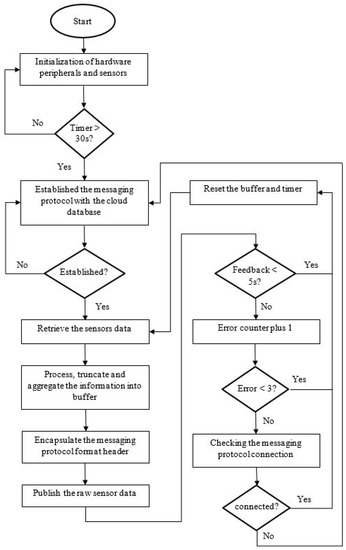
Figure 2. Flow Process of the Overall Operation Sequence.

The collected data is processed and sorted in the cloud database. Device nodes located in the vehicle cabin are assigned their unique identifier (ID) to avoid any mislocation of data entry. Furthermore, a database handler is developed to reject distorted data entry and invalid device ID. Finally, a web page display is developed to view the real-time sensor data of air quality status in the vehicle cabin. The visualization helps users to learn the data patterns of the in-vehicle air quality system.

3.2. Sensor Development

Figure 3 presents the hardware of the device node. The hardware power supply is supplied using the in-car charger, where the voltage ranges from 11.9 V to 14.8 V. From the experiment, it can be seen that the voltage value is not fixed. The value fluctuates from time to time within the voltage range. A step-down process is then performed using a transformer in the device, to allow the use of different voltage supplies from the sensors. These sensors only need 3.8 V to operate. Therefore, a step-down process is important to avoid a short circuit and subsequently damaging the device node.

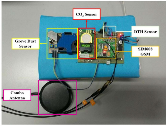
Figure 3. Development of Sensors in the Device Node.

3.3. Air Quality Prediction

In this study, the output of the prediction system is based on the air quality index (AQI). It acts as an indicator to determine whether the environment is composed of air pollutants that can affect human health. The study selects several parameters such as CO₂ and particulate matter (PM_2.5 and PM₁₀) as well as time, latitude, longitude and speed. Based on the identified parameters, the study proposes to predict the future index of air quality inside the vehicle cabin, using an established indoor air quality standard as a guide. Table 3 shows the pollutants concentration guidelines used to obtain the AQI value.

Table 3. Concentration Value for Measuring AQI.

CO2 (ppm)	PM2.5 (µg/m3)e	PM10 (µg/m3)e	AQI	Five Bands of AQI
BPlow-BPhigh	BPlow-BPhigh	BPlow-BPhigh	Ilow-Ihigh
400–600	0.0–12.0	0–54	0–50	Good
601–1000	12.1–35.4	55–154	51–100	Moderate
1001–1500	35.5–55.4	155–254	101–150	Unhealthy for sensitive group
1501–2500	55.5–150.4	255–354	151–200	Unhealthy
2501–5000	150.5–250.4	355–424	201–500	Very unhealthy

The function of the value concentration is to classify and indicate the risk of adverse health effects on the occupants. Using Table 3, the in-vehicle air quality parameters can be categorized into five bands to form their own class of AQI. Each of the bands has a value to represent the air quality of a specific air parameter. The value of AQI can be calculated using Equation (1). For example, the air sensor reading is recorded as CO₂ = 1600 ppm, PM_2.5 = 11.3 µg/m³ and PM₁₀ = 39 µg/m³. Each of the parameters will be calculated using Equation (1). After the calculation, CO₂, PM_2.5 and PM₁₀ fall into the AQI of band four (155.8), band one (12.1) and band one (36.1), respectively.

$$\mathrm{AQI}=\frac{I_{Hi}-I_{Lo}}{B{P}_{Hi}-B{P}_{Lo}} \left(C_p-B{P}_{Lo}\right)+I_{Lo}$$

(1)

where

$C_p$ = the rounded concentration of pollutant p

$B{P}_{Hi}$ = the breakpoint that is greater than or equal to $C_p$

$B{P}_{Lo}$ = the breakpoint that is less than or equal to $C_p$

$I_{Hi}$ = the AQI value corresponding to $B{P}_{Hi}$

$I_{Lo}$ = the AQI value corresponding to $B{P}_{Lo}$

3.4. Data Collection

The data collection is conducted inside the vehicle cabin. The duration of the data collection process is approximately two months, with an average usage of two hours each day. The experiments are performed using built-in sensors located in the car cabin, as in Figure 4.

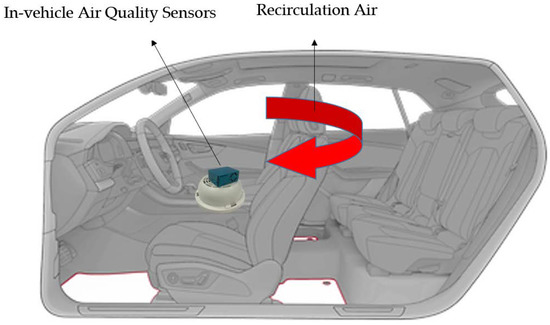
Figure 4. Representation of Sensor Device in Vehicle Cabin.

The sensors are powered up using an in-car adapter charger and placed between the driver seat and passenger seat. The cabin condition is set to recirculation mode with the air conditioner always turned on. This is to make sure that it represents the real-life scenarios of drivers while driving the car. The experiment is then separated into two different time slots. Firstly, data is taken in the morning, between 06:00 and 08:00. Another set of experiments is then conducted in the evening, between 13:00 and 15:00. Overall, the traveling distance during the experiments reached a total of 875 km for 19 days (between June 2019 and July 2019). Figure 5 shows the average daily traveling distance, which was approximately 46.1 km per day. Meanwhile, Table 4 depicts the overall size of data samples that were collected, based on monthly and periodic sections throughout the data collection process.

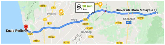
Figure 5. Daily Traveling Distance for Data Collection.

Table 4. Description of data features and sample sizes for data collection process.

Collection Site		Parameter
Monthly	Number of records	48,816
	Size	3,593,866 bytes (3.59 MB)
One section	Number of records	1184
	Size	92,160 bytes (0.09 MB)
Value types		Twelve air quality variables (time, latitude, longitude, speed, CO2, temperature, humidity, PM1, PM2.5, PM10, count, label)

4. Prediction Models

4.1. Data Pre-Processing

The initial stage of developing an efficient prediction model is the data pre-processing, which consists of data cleaning, data labelling and data normalization. Data pre-processing is needed as it can help to clean the data and take significant patterns before giving them to the prediction models. This is because the collected sensor data consists of noisy and meaningless information and sensor errors which are known as outliers, as well as missing data. Thus, improper processing of the datasets can lead to inaccurate and unreliable prediction models which result in underperformed performance rates of the predictive or classification model.

In the data pre-processing, the data cleaning process is first performed. The task uses the nearest-neighbor interpolation method. The method is suitable for datasets that have missing values or outlier conditions. Equation (2) shows the mathematical formula for the nearest-neighbor method [40]. When any of the outlier values occur in position x_i, the value of the closest known neighbor is then used to substitute the outlier value. Moreover, if the number of outliers is greater than five, the average of the five previous data will then be used to substitute back in the original outlier values.

$$x_i=\{\begin{array}{c} \frac{x_{i-1}+x_{i-2}}{2} , if i=2;\\ \frac{x_{i-1}+x_{i-2}+x_{i-3}}{3} , if i=3;\\ \frac{x_{i-1}+x_{i-2}+x_{i-3}+x_{i-4}}{4} , if i=4;\\ \frac{x_{i-1}+x_{i-2}+x_{i-3}+x_{i-4}+x_{i-5}}{5} , otherwise \end{array}$$

(2)

where $x_i$ is the outlier value.

Data labelling is the second part of the data pre-processing step. The process is needed as the prediction model uses the supervised learning approach, in which the model should have a ground truth or a set of labelling output data. The labelled data functions for the orientation of the training and testing process for the target in the AI predictive model. Multiple raw data from the device node in the vehicle cabin such as CO₂, PM_2.5, PM₁₀, vehicle speed, temperature, and humidity are used as the input data. The output data is calculated using the air quality index stated in [41]. Subsequently, data normalization is implemented to help the prediction model to capture the significant patterns. The function of the normalization process is to convert the numeric values in the dataset into a set with 0 to 1 range. The process is conducted without changing the original characteristics of the dataset. In this study, the normalization procedure uses the Min-Max method.

4.2. Deep Learning Models

The study uses two types of algorithms from machine learning and two algorithms from deep learning methods. The models are used to predict the state of the air quality index inside the car cabin. They are built based on historical data collected over two months.

The proposed approach is divided into machine learning algorithms of SVR and MLP, while deep learning methods are composed of LSTM and GRU models. These models are chosen as they provide a good performance when dealing with time-series data. Furthermore, the real-world dataset that is used in this study is composed of a three-dimensional data structure with timestamps associated with each of the sensor readings. Therefore, the use of LSTM and GRU is the most suitable learning model that can handle the time-series data.

The learning model utilizes data from sensors such as CO₂, PM_2.5, PM₁₀, vehicle speed, temperature, and humidity. Firstly, the data from these sensors are presented in the two-dimensional data representation. After this, multiple rows are combined to create a set of three-dimensional data, as shown in Figure 6.

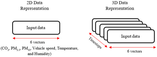
Figure 6. Input Data Representation.

The structure of this multiple sequence prediction method is used to predict air quality in a step-by-step sequence. To predict value X ̂_(t + 1) at timestamp t + 1, previous historical data X_1, X_2, X_3, …, X_t, which are known as time lags, are required. When generating the next prediction value of X ̂_(t + 2), X ̂_(t + 1), data is fed back into the dataset. The process flow will continue until the designed moving windows are completed. The GRU model is composed of three hidden layers with a sigmoid activation function applied to each layer. The output layer is computed using a dense function, which compresses the three-dimensional data to one-dimensional data. Adam optimization is then implemented in the training model to calculate the probabilistic errors between the ground truth and output of the prediction model. Figure 7 shows the proposed overall structure for the deep learning model. It is implemented in the multiple sequence prediction task.

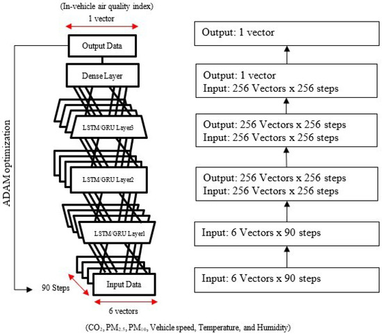
Figure 7. Prediction of Multiple Sequence using GRU and LSTM.

4.3. Hyperparameter Testing

The next step is to set the hyper-parameters for the prediction model to work effectively. The efficiency of the model could be affected based on the parameter settings of the model. For example, learning rate, number of hidden nodes and hidden layers play an important part in building an effective prediction model. If the value is not in the optimum mode, the output of the learning model may contribute to overfitting problems. In this study, the grid-search method is utilized to find the optimum parameters of the learning model that can be used. The method employs an optimization algorithm that can select the best parameters by dividing the domain of the hyper-parameters into a discrete grid. Then, the performance metrics of the model are calculated in each grid, using the cross-validation tool. Table 5 presents the range of hyperparameters that are determined and applied in the predictive models.

Table 5. Range of Hyperparameters of the Predictive Model.

Hyperparameter	Value
Hidden layer	{1–5}
Hidden node	{23–210}
Learning rate	{0.001, 0.005, 0.01, 0.05, 0.1, 0.5}
Iteration	{23–212}
Split	{0.7, 0.8}

5. Experimental Results

The comparison process was performed to evaluate which approaches gave the best performances. It was carried out between the machine learning and deep learning models. The machine learning algorithm was represented by SVR and MLP, while deep learning models were comprised of LSTM and GRU, which are the variant models from Recurrent Neural Network (RNN). In this paper, SVR and MLP are regarded as the machine learning approach because they have not been provided with the recurrence feedback to update the weight and bias. However, for the deep learning approach, both the LSTM and GRU models were provided with recurrent feedback to improve the weight and bias values that were used.

The hyperparameter values were decided using the grid-search method. Table 6 presents the specific value of the hyperparameters that were applied using the grid-search method. It can be seen that tuning in these parameters impacts greatly the prediction results. The structures of MLP, LSTM and GRU are much more similar, as they are composed of a similar branch of learning model, while SVR is different in terms of different parameters such as kernel, kernel coefficient, and regularization parameter.

Table 6. Hyperparameters Implemented in the Prediction Task.

Hyperparameters	Machine Learning		Deep Learning
	SVR	MLP	LSTM	GRU
Kernel	RBF	-	-	-
Regularization	501.19	-	-	-
Hidden layer	1	1	3	3
Hidden node	-	128	64 + 512 + 128	64 + 512 + 256
Learning rate	0.001	0.001	0.01	0.001
Iteration	10,000	2000	1500	1800
Split	0.8	0.8	0.8	0.8
Optimizer	-	Gradient descent	Adam	Adam
Activation Function	-	Sigmoid	Hyperbolic tangent	Hyperbolic tangent

The next process was to build the prediction models with the predefined hyperparameters that were determined in the previous process. The collected data was used to build the proposed models. The input for the training and validation model was divided into 80% and 20%, respectively. The training data were also based on the section and monthly data. Table 7 presents the performance of the proposed models validated by the section and monthly data. The result clearly shows that the SVR with RBF kernel and GRU models had almost the same performance index in the evaluation results. However, the proposed GRU prediction model presented much higher performance rates in terms of prediction accuracy and reduced error rates. The GRU model obtained the R² value of 0.83 for the section data and 0.97 for the monthly data.

Table 7. Overall Results of Proposed Model based on Section and Monthly Data.

Data	Evaluation	Machine Learning		Deep Learning
		SVR	MLP	LSTM	GRU
Section	R2	0.83	0.57	0.65	0.83
	MSE	126.43	453.31	263.48	121.84
	RMSE	11.24	37.23	16.23	11.04
	MAE	1.52	21.98	1.93	1.55
Monthly	R2	0.96	0.72	0.96	0.97
	MSE	23.62	212.48	28.18	6.45
	RMSE	4.86	14.58	5.31	2.54
	MAE	0.97	11.57	0.82	0.95

Lastly, the final step was to evaluate the performance of the prediction of in-vehicle air quality. Table 8 shows the results of the future prediction data. It compares the three types of time periods: five minutes, ten minutes and twenty minutes. It can be seen that the prediction of the five-minute data had a slightly higher performance rate, compared with the ten- and twenty-minute data predictions. The results also show that the proposed GRU prediction model gave a very stable evaluation performance across the three types of data. Meanwhile, Figure 8 shows the graph visualization of the prediction results, using the proposed GRU prediction models compared with the actual data.

Table 8. Results of Prediction Data for Three Types of data.

Time (min)	Evaluation	Machine Learning		Deep Learning
		SVR	MLP	LSTM	GRU
5	R2	0.02	0.00077	0.81	0.97
	MSE	833.67	249.43	160.49	23.63
	RMSE	28.87	16.08	12.67	4.86
	MAE	23.48	248.77	248.77	0.95
10	R2	0.0005	0.013	0.76	0.96
	MSE	865.99	251.09	205.02	26.93
	RMSE	29.51	16.08	12.67	5.19
	MAE	23.39	248.77	248.77	1.01
20	R2	0.0003	0.013	0.74	0.92
	MSE	923.8	251.09	189.62	55.78
	RMSE	30.39	16.08	13.77	7.47
	MAE	24.18	248.77	2.1	1.18

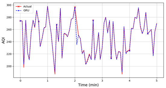
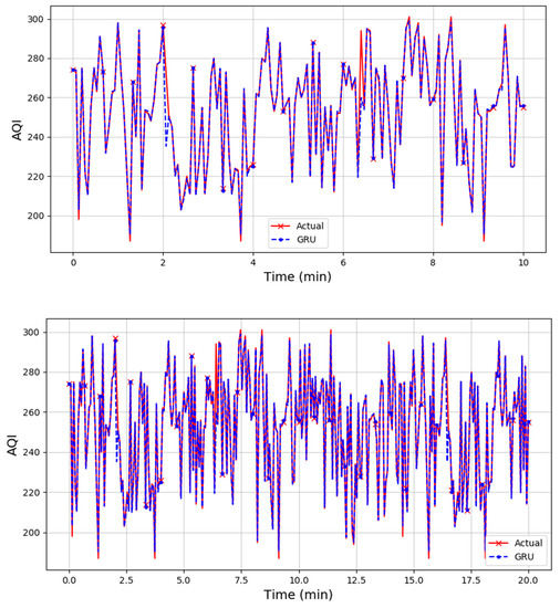
Figure 8. Comparison of Prediction Results using GRU Prediction Model with Actual Data.

6. Conclusions

After an extensive series of experiments, it can be concluded that the GRU model from the deep learning approach gives a good performance in predicting in-vehicle air quality. The model was compared with the LSTM model as well as with SVR and MLP from the traditional machine learning models. The proposed model achieved the highest prediction error of 0.97 for R². Furthermore, the GRU model also showed the lowest error in terms of MSE, RMSE and MAE. From these experiments, it can be seen that the performance of the prediction system depends on the time taken to collect the data. From the result, the GRU model with five-minute data had the highest performance compared with the ten- and twenty-minute data.

Moreover, the model’s hyperparameters were also optimized using the grid-search method. This allowed the optimum value to be used for the model to predict air quality. The overall results showed that the GRU model was able to capture the historical data of installed sensors and predict them successfully. However, some limitations were noted throughout the study. It can be seen that some data are missing due to the loss of internet connectivity. Furthermore, the in-vehicle system needs to be provided with reliable communication systems in order to provide an efficient prediction system

For future work, the model will be embedded in the cloud database for faster data processing. This task can be extended to various applications of prediction systems for smart mobility applications. Furthermore, the feature extraction process can be conducted before performing the prediction task. The goal is to autonomously extract relevant features for representing environmental conditions and to compare the performance rates with non-extracted feature methods.

References

- World Health Organization (WHO). World Health Statistics 2017; WHO: Geneva, Switzerland, 2017; Volume 91. [Google Scholar]
- Gross, A. New Study Reveals When, Where and How Much Motorists Drive; American Automobile Association: Washington, DC, USA, 2015. [Google Scholar]
- Hudda, N.; Fruin, S.A. Carbon dioxide accumulation inside vehicles: The effect of ventilation and driving conditions. Sci. Total Environ. 2018, 610–611, 1448–1456. [Google Scholar] [CrossRef] [PubMed]
- Brodzik, K.; Faber, J.; Łomankiewicz, D.; Gołda-Kopek, A. In-vehicle VOCs composition of unconditioned, newly produced cars. J. Environ. Sci. 2014, 26, 1052–1061. [Google Scholar] [CrossRef]
- Harik, G.; El-Fadel, M.; Shihadeh, A.; Alameddine, I.; Hatzopoulou, M. Is in-cabin exposure to carbon monoxide and fine particulate matter amplified by the vehicle’s self-pollution potential? Quantifying the rate of exhaust intrusion. Transp. Res. Part D Transp. Environ. 2017, 54, 225–238. [Google Scholar] [CrossRef]
- Thriumani, R.; Zakaria, A.; Hashim YZ, H.Y.; Jeffree, A.I.; Helmy, K.M.; Kamarudin, L.M.; Omar, M.I.; Shakaff, A.Y.M.; Adom, A.H.; Persaud, K.C. A study on volatile organic compounds emitted by in-vitro lung cancer cultured cells using gas sensor array and SPME-GCMS. BMC Cancer 2018, 18, 362. [Google Scholar] [CrossRef]
- Mathur, G. Use of Partial Recirculation to Limit Build-Up of Cabin Carbon Dioxide Concentrations to Safe Limits per ASHRAE Standard-62; SAE Technical Paper; SAE International: Warrendale, PA, USA, 2020. [Google Scholar] [CrossRef]
- Szczurek, A.; Maciejewska, M. Categorisation for air quality assessment in car cabin. Transp. Res. Part D Transp. Environ. 2016, 48, 161–170. [Google Scholar] [CrossRef]
- Zhang, X.; Wargocki, P.; Lian, Z. Human responses to carbon dioxide, a follow-up study at recommended exposure limits in non-industrial environments. Build. Environ. 2016, 100, 162–171. [Google Scholar] [CrossRef]
- Permentier, K.; Vercammen, S.; Soetaert, S.; Schellemans, C. Carbon dioxide poisoning: A literature review of an often forgotten cause of intoxication in the emergency department. Int. J. Emerg. Med. 2017, 10, 17–20. [Google Scholar] [CrossRef]
- Sánchez-Corcuera, R.; Nuñez-Marcos, A.; Sesma-Solance, J.; Bilbao-Jayo, A.; Mulero, R.; Zulaika, U.; Azkune, G.; Almeida, A. Smart cities survey: Technologies, application domains and challenges for the cities of the future. Int. J. Distrib. Sens. Netw. 2019, 15, 1–36. [Google Scholar] [CrossRef]
- Dass, A.; Srivastava, S.; Chaudhary, G. Air pollution: A review and analysis using fuzzy techniques in Indian scenario. Environ. Technol. Innov. 2021, 22, 101441. [Google Scholar] [CrossRef]
- Barnes, N.M.; Ng, T.; Ma, K.K.; Lai, K.M. In-cabin air quality during driving and engine idling in air-conditioned private vehicles in Hong Kong. Int. J. Environ. Res. Public Health 2018, 15, 611. [Google Scholar] [CrossRef]
- Baldi, T.; Delnevo, G.; Girau, R.; Mirri, S. On the Prediction of Air Quality within Vehicles using Outdoor Air Pollution: Sensors and Machine Learning Algorithms. Assoc. Comput. Mach. 2022, NET4us ’22, 14–19. [Google Scholar]
- Pushpam, V.S.E.; Kavitha, N.S.; Karthik, A.G. IoT Enabled Machine Learning for Vehicular Air Pollution Monitoring. In Proceedings of the 2019 International Conference on Computer Communication and Informatics, ICCCI, Coimbatore, India, 23–25 January 2019. [Google Scholar] [CrossRef]
- Angelova, R.A.; Markov, D.G.; Simova, I.; Velichkova, R.; Stankov, P. Accumulation of metabolic carbon dioxide (CO2) in a vehicle cabin. IOP Conf. Ser. Mater. Sci. Eng. 2019, 664, 012010. [Google Scholar] [CrossRef]
- Kirimtat, A.; Krejcar, O.; Kertesz, A.; Tasgetiren, M.F. Future Trends and Current State of Smart City Concepts: A Survey. IEEE Access 2020, 8, 86448–86467. [Google Scholar] [CrossRef]
- Xu, B.; Chen, X.; Xiong, J. Air quality inside motor vehicles’ cabins: A review. Indoor Built Environ. 2018, 27, 452–465. [Google Scholar] [CrossRef]
- Satish, U.; Mendell, M.J.; Shekhar, K.; Hotchi, T.; Sullivan, D.; Streufert, S.; Fisk, W.J. Is CO2 an indoor pollutant? direct effects of low-to-moderate CO2 concentrations on human decision-making performance. Environ. Health Perspect. 2012, 120, 1671–1677. [Google Scholar] [CrossRef]
- Kadiyala, A.; Ashok, K. Vector Time Series-Based Radial Basis Function Neural Network Modeling of Air Quality Inside a Public Transportation Bus Using Available Software. Environ. Prog. Sustain. Enegy 2017, 36, 4–10. [Google Scholar] [CrossRef]
- Hable-Khandekar, V.; Srinath, P. Machine Learning Techniques for Air Quality Forecasting and Study on Real-Time Air Quality Monitoring. In Proceedings of the 2017 International Conference on Computer, Communication, Control and Automatisation, ICCUBEA, Pune, India, 17–18 August 2017. [Google Scholar] [CrossRef]
- Jung, H. Modeling CO2 concentrations in vehicle cabin. SAE Tech. Pap. 2013, 2, 1–6. [Google Scholar] [CrossRef]
- Lohani, D.; Acharya, D. Real time in-vehicle air quality monitoring using mobile sensing. In Proceedings of the 2016 IEEE Annual India Conference INDICON, Bangalore, India, 16–18 December 2016; pp. 1–5. [Google Scholar] [CrossRef]
- Santana, P.; Almeida, A.; Mariano, P.; Correia, C.; Martins, V.; Almeida, S.M. Air quality mapping and visualisation: An affordable solution based on a vehicle-mounted sensor network. J. Clean. Prod. 2021, 315, 128194. [Google Scholar] [CrossRef]
- Russi, L.; Guidorzi, P.; Pulvirenti, B.; Aguiari, D.; Pau, G.; Semprini, G. Air Quality and Comfort Characterisation within an Electric Vehicle Cabin in Heating and Cooling Operations. Sensors 2022, 22, 543. [Google Scholar] [CrossRef]
- Rani, N.L.A.; Azid, A.; Khalit, S.I.; Juahir, H.; Samsudin, M.S. Air pollution index trend analysis in Malaysia, 2010-15. Pol. J. Environ. Stud. 2018, 27, 801–808. [Google Scholar] [CrossRef]
- Rahman, N.H.A.; Lee, M.H. Air pollutant index calendar-based graphics for visualizing trends profiling and analysis. Sains Malays. 2020, 49, 201–209. [Google Scholar] [CrossRef]
- Cui, Y.; Xu, Y.; Wu, D. EEG-Based Driver Drowsiness Estimation Using Feature Weighted Episodic Training. IEEE Trans. Neural Syst. Rehabil. Eng. 2019, 27, 2263–2273. [Google Scholar] [CrossRef] [PubMed]
- Verma, B.; Choudhary, A. Deep Learning Based Real-Time Driver Emotion Monitoring. In Proceedings of the 2018 IEEE International Conference on Vehicular Electronics and Safety, ICVES, Madrid, Spain, September 2018; pp. 12–14. [Google Scholar] [CrossRef]
- Lohani, D.; Barthwal, A.; Acharya, D. Modeling vehicle indoor air quality using sensor data analytics. J. Reliab. Intell. Environ. 2022, 8, 105–115. [Google Scholar] [CrossRef]
- EPA. NAAQS Table; US Environmental Protection Agency: Washington, DC, USA, 2016.
- Manisalidis, I.; Stavropoulou, E.; Stavropoulos, A.; Bezirtzoglou, E. Environmental and Health Impacts of Air Pollution: A Review. Front. Public Health 2020, 8, 14. [Google Scholar] [CrossRef] [PubMed]
- DOSH. Industry Code of Practice on Indoor Air Quality 2010; Ministry of Human Resources Department of Occupational Safety and Health: Putrajaya, Malaysia, 2010; pp. 1–50.
- Hussein, W.N.; Kamarudin, L.M.; Hussain, H.N.; Hamzah, M.R.; Jadaa, K.J. Technology elements that influence the implementation success for big data analytics and IoT-oriented transportation system. Int. J. Adv. Trends Comput. Sci. Eng. 2019, 8, 2347–2352. [Google Scholar] [CrossRef]
- Sukor, A.S.A.; Zakaria, A.; Rahim, N.A. Activity recognition using accelerometer sensor and machine learning classifiers. In Proceedings of the 2018 IEEE 14th International Colloquim on Signal Processing & Its Application, Penang, Malaysia, 9–10 March 2018; pp. 233–238. [Google Scholar] [CrossRef]
- Sukor, A.S.A.; Zakaria, A.; Rahim, N.A.; Kamarudin, L.M.; Nishizaki, H. Abnormality Detection Approach using Deep Learning Models in Smart Home Environments. In Proceedings of the International Conference on Communications and Broadband Networking, ICCBN, Nagoya, Japan, 12–15 April 2019; pp. 22–27. [Google Scholar] [CrossRef]
- Almaleeh, A.S.; Zakaria, A.A.A. A Review on the efficiency and accuracy of localization of moisture distributions sensing in agricultural silos. IOP Conf. Ser. Mater. Sci. Eng. 2019, 705, 012054. [Google Scholar] [CrossRef]
- Xayasouk, T.; Lee, H.M.; Lee, G. Air pollution prediction using long short-term memory (LSTM) and deep autoencoder (DAE) models. Sustainability 2020, 12, 2570. [Google Scholar] [CrossRef]
- Athira, V.; Geetha, P.; Vinayakumar, R.; Soman, K.P. DeepAirNet: Applying Recurrent Networks for Air Quality Prediction. Procedia Comput. Sci. 2018, 132, 1394–1403. [Google Scholar] [CrossRef]
- Lepot, M.; Aubin, J.B.; Clemens, F.H.L.R. Interpolation in time series: An introductive overview of existing methods, their performance criteria and uncertainty assessment. Water 2017, 9, 796. [Google Scholar] [CrossRef]
- Goh, C.C.; Kamarudin, L.M.; Zakaria, A.; Nishizaki, H.; Ramli, N.; Mao, X.; Zakaria, S.M.M.S.; Kanagaraj, E.; Sukor, A.S.A.; Elham, M.F. Real-time in-vehicle air quality monitoring system using machine learning prediction algorithm. Sensors 2021, 21, 4956. [Google Scholar] [CrossRef]
Publisher’s Note: MDPI stays neutral with regard to jurisdictional claims in published maps and institutional affiliations. |
© 2022 by the authors. Licensee MDPI, Basel, Switzerland. This article is an open access article distributed under the terms and conditions of the Creative Commons Attribution (CC BY) license (https://creativecommons.org/licenses/by/4.0/).