
Review of Long-Term Trends in the Equatorial Ionosphere Due the Geomagnetic Field Secular Variations and Its Relevance to Space Weather

 , and
, and 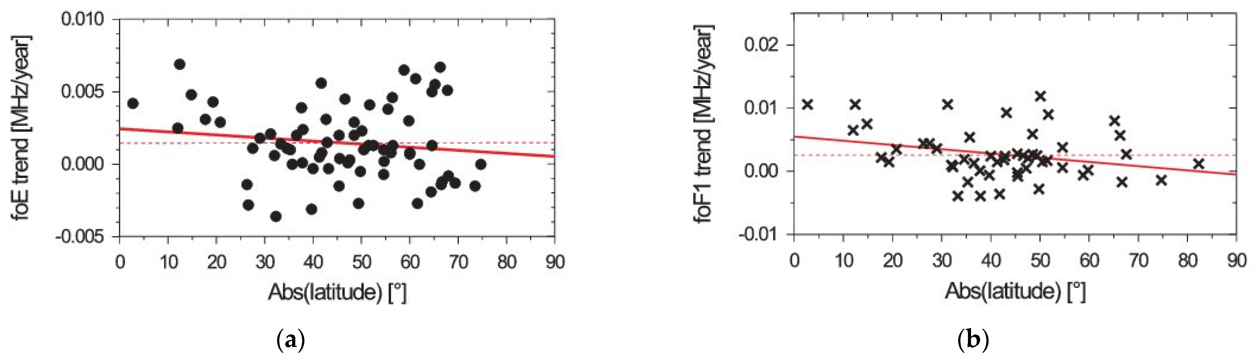
Abstract
1. Introduction
2. Setting the Scene
2.1. Equatorial and Low-Latitude Ionosphere Distinctive Characteristics
- the equatorial ionization anomaly (EIA) in the F2 region which consists of a trough of ionization density centered on the magnetic equator and crests at 15 to 20° to the north and south;
- possible additional stratification: F3 layer;
- the strong enhancement of the horizontal conductance at the dynamo region (E-region) which results in a strong current: the equatorial electrojet (EEJ), and also in an enhanced daily variation in H at the Earth’s surface (ΔH); and
- equatorial spread F or equatorial plasma bubbles (EPBs).
2.2. Secular Variation of the Earth’s Magnetic Field at Geographic Low Latitudes
2.3. Simple Mechanisms Linking Geomagnetic Field Variation to Ionospheric Consequences
2.3.1. Transport Effects
2.3.2. Conductivity Effects
2.3.3. Equatorial Electrojet Current Effects
2.3.4. Magnetic Daily Variation Due to the Equatorial Electrojet Effects
3. Long-Term Trends Based on Experimental Data
3.1. Ionospheric D Layer
3.2. Ionospheric E and F1 Layers Peak Electron Density and Height
- Changes in the auroral ovals, which may result in an increase or decrease of a station’s position relative to the auroral oval. This is linked to an increase or decrease, respectively, of energetic charged particles’ precipitation from the magnetosphere which in turn generate nitric oxide (NO) that at E-region altitudes can produce an increase in ionization loss rate and hence a decrease in the E-region electron concentration.
- The ratio of the geomagnetic field strength at 110 km to that at equatorial minimum on the same field line determines the particle loss cone, which could affect foE also through changes in charged particle precipitation.
- The dip angle and declination could have a more direct effect on foE because they have some controlling influence over plasma motion, even though they really become effective at the F2 layer, where transport processes gain importance in the continuity equation.
- Geomagnetically, conjugate points to a given station may be changing their latitude in the opposite hemisphere and hence altering the secondary ionization being transported along the field line between hemispheres.
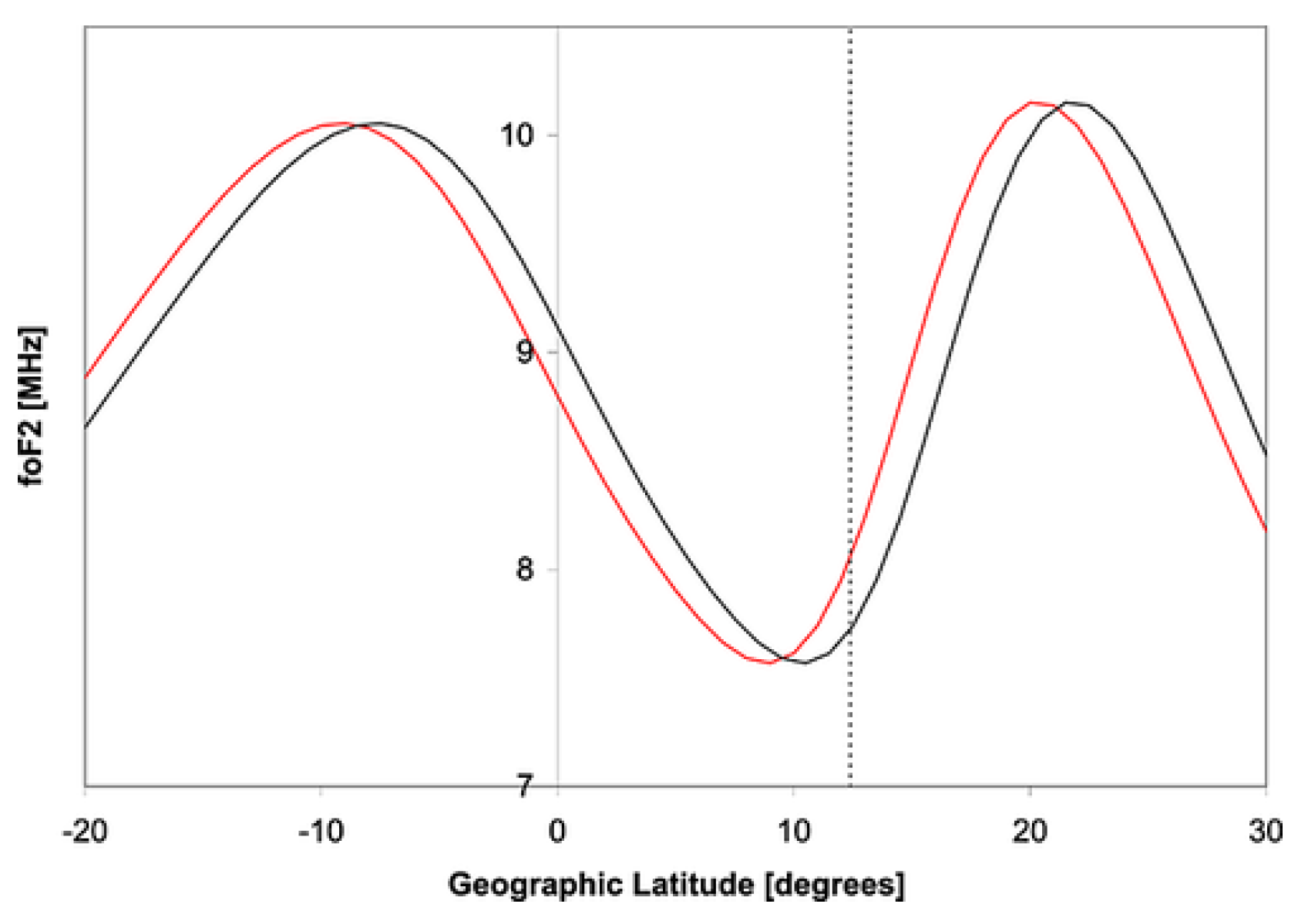
3.3. Ionospheric F2-Layer Peak Electron Density and Height
3.4. Topside Ionosphere
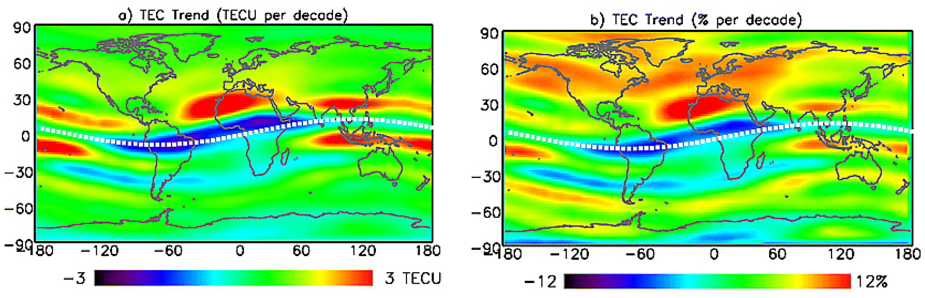
3.5. Ionosphere Total Electron Content (TEC)
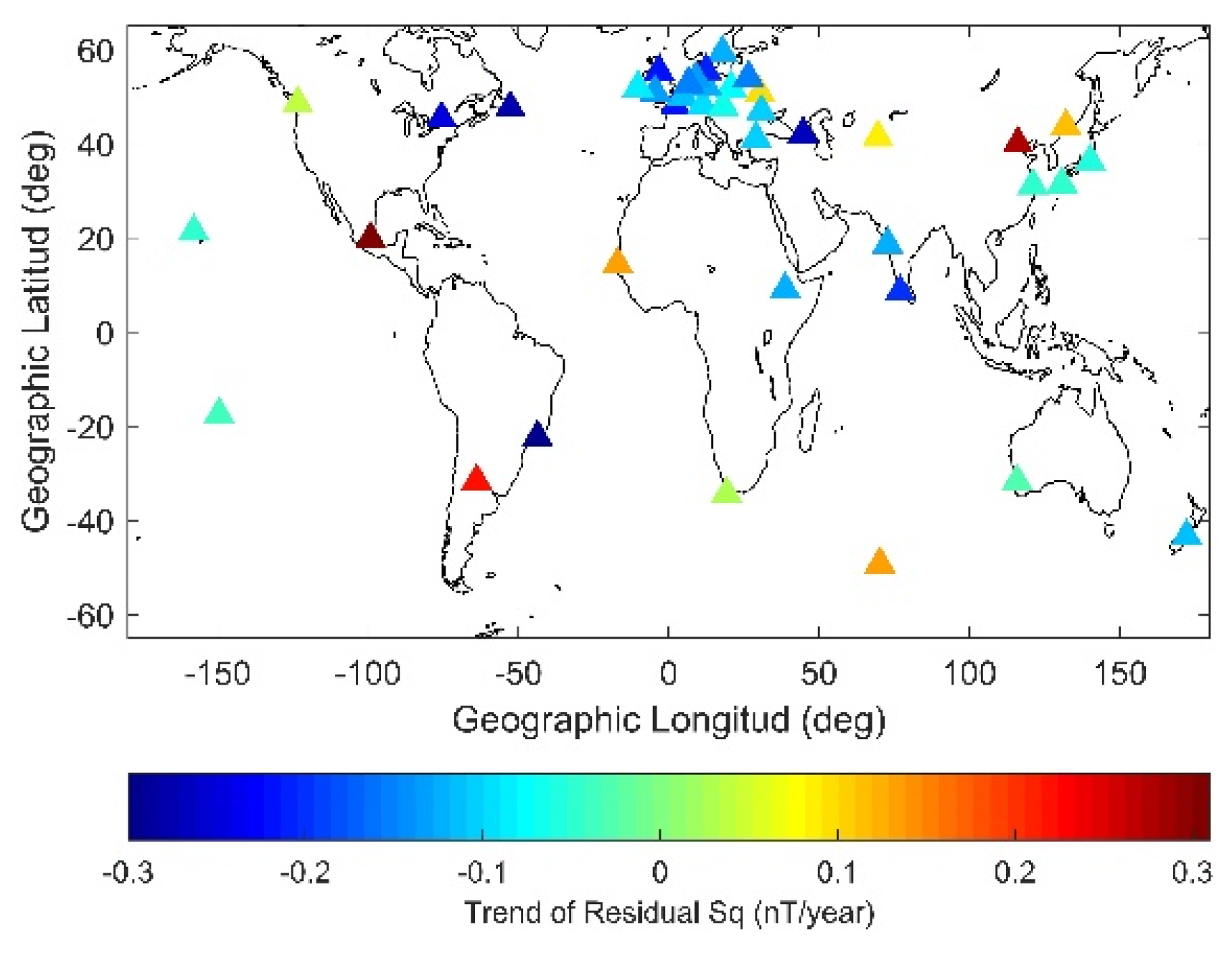
3.6. Ionospheric Currents: Sq and EEJ
3.7. F3 and Sporadic E Layers
3.8. Warnings for Experimental Trends’ Assessment
4. Long-Term Trends Based on Theoretical Analysis and Modeling
4.1. Modeling Using IGRF
4.2. Modeling Using a Pure Dipolar field
4.3. Warnings for Theoretical and Model Trends Assessment and Simulations
5. Conclusions
- (1)
- the relatively low number of equatorial and low-latitude stations with long-enough data records in order to obtain statically significant results, and
- (2)
- the important role played by dynamics due to the special geometry of the Earth’s magnetic field at this very special region, which combines with feedbacks and neutral winds and tides complicating models and making it difficult to obtain reliable results.
5.1. Controversies and Gaps
- (1)
- On one side, that linked to experimental data. As already mentioned, the number of equatorial and low-latitude stations with long data series is not enough to obtain a thorough picture of trend spatial pattern at these zonal regions.
- (2)
- On the other side, that linked with modeling. The consideration of the magnetic equator displacement as a trend source should sometimes be considered separately from the effect of secular variations in traditional geomagnetic field parameters, such as its intensity, I and D.
- (3)
- In addition, there are gaps dealing with the complexity of models needed to simulate the scenario of the ionosphere at equatorial and low-latitudes and the complexity of the magnetic field variation itself, which is not easy to consider fully. The proof of this is that most of the models consider a pure dipolar magnetic field instead of the “true” field.
5.2. Recommendations for Future Studies
- (1)
- Obtaining a regional picture from experimental data: even though trend investigations in the equatorial and low-latitude ionosphere suffer from insufficient geographical coverage, a regional picture can be obtained through a comprehensive analysis of the data available, with the help of new and better statistical tools.
- (2)
- Smaller scale analysis of the spatial distribution of trends: this should be done taking into account the different velocity and directions of the magnetic equator displacement along the last decades, which seems to induce stronger trends than those induced by changes in I, D, and/or B.
- (3)
- Analysis of the geomagnetic activity effect in long term trends: this is closely linked to space weather and refers to considering not only trends in the activity itself, but in its efficiency in producing ionospheric modifications based on geomagnetic position secular changes of a given geographic position.
- (4)
- More detailed, quantitative comparisons between simulated and observed trends: this is still needed to determine more precisely the relative contribution of magnetic field changes to observed trends compared to other drivers. Especially the increase in greenhouse gas concentrations, whose region of effectiveness is much wider than the region assumed to be more strongly affected by the Earth’s magnetic field.
- (5)
- Analysis of possible connection with high geomagnetic latitudes: since other regions expected to be strongly affected by the secular variation of the Earth’s magnetic field are those close to the auroral zones and polar caps through the changes expected in charged particles precipitation. It would be interesting to analyze if there is any association between changes at low and high latitudes considering a common forcing trend mechanism.
- (6)
- Analysis of the dipole center displacement effect isolated from other Earth’s magnetic field variations. Considering that there are studies which analyze the isolated effect of the Earth’s magnetic field dipolar moment decrease, and of the variation in the main dipole axis inclination, it would be interesting to see the effect of the isolated variation of the main dipole axis center displacement from the Earth’s center, besides its known effect on the South Atlantic Anomaly.
- (7)
- The incorporation of more sophisticated computational models in the interaction of the Sun–Earth system for trend studies: in fact, considering that computational advances are so prosperous since the last years, they will surely serve to deepen the study of secular geomagnetic field effects over the ionosphere and its competing role with the anthropogenic effect at low latitudes, a topic that is still current and more interesting than ever, taking into account the accelerated decline of the dipole field in recent decades.
Author Contributions
Funding
Institutional Review Board Statement
Informed Consent Statement
Data Availability Statement
Acknowledgments
Conflicts of Interest
References
- Rishbeth, H.; Garriott, O.K. Introduction to Ionospheric Physics; Academic Press: New York, NY, USA, 1969. [Google Scholar]
- Roble, R.G.; Dickinson, R.E. How will changes in carbon dioxide and methane modify the mean structure of the mesosphere and thermosphere? Geophys. Res. Lett. 1989, 16, 1441–1444. [Google Scholar] [CrossRef]
- Rishbeth, H. A greenhouse effect in the ionosphere? Planet. Space Sci. 1990, 38, 945–948. [Google Scholar] [CrossRef]
- Laštovička, J.; Solomon, S.; Qian, L. Trends in the Neutral and Ionized Upper Atmosphere. Space Sci. Rev. 2012, 168, 113–145. [Google Scholar] [CrossRef]
- Laštovička, J.; Beig, G.; Marsh, D.R. Response of the mesosphere-thermosphere-ionosphere system to global change-CAWSES-II contribution. Prog. Earth Planet. Sci. 2014, 1, 21. [Google Scholar] [CrossRef]
- Laštovička, J. A review of recent progress in trends in the upper atmosphere. J. Atmos. Solar-Terr. Phys. 2017, 163, 2–13. [Google Scholar] [CrossRef]
- Lastovicka, J. Long-Term Trends in the Upper Atmosphere, in Upper Atmosphere Dynamics and Energetics; Wang, W., Zhang, Y., Paxton, L.J., Eds.; American Geophysical Union: Washington, DC, USA, 2021; pp. 325–344. [Google Scholar]
- Elias, A.G. Trends in the F2 ionospheric layer due to long-term variations in the Earth’s magnetic field. J. Atmos. Solar Terr. Phys. 2009, 71, 1602–1609. [Google Scholar] [CrossRef]
- Cnossen, I. The importance of geomagnetic field changes versus rising CO2 levels for long-term change in the upper atmos-phere. J. Space Weather Space Clim. 2014, 4, A18. [Google Scholar] [CrossRef]
- Cnossen, I. Analysis and attribution of climate change in the upper atmosphere from 1950 to 2015 simulated by WACCM-X. J. Geophys. Res. 2020, 125, e2020JA028623. [Google Scholar] [CrossRef]
- Matzka, J.; Siddiqui, T.A.; Lilienkamp, H.; Stolle, C.; Veliz, O. Quantifying solar flux and geomagnetic main field influence on the equatorial ionospheric current system at the geomagnetic observatory Huancayo. J. Atmos. Solar-Terr. Phys. 2017, 163, 120–125. [Google Scholar] [CrossRef]
- Zossi, B.S.; Elias, A.G.; Fagre, M. Ionospheric Conductance Spatial Distribution During Geomagnetic Field Reversals. J. Geophys. Res. Space Phys. 2018, 12, 2379–2397. [Google Scholar] [CrossRef]
- Fagre, M.; Zossi, B.S.; Yiğit, E.; Amit, H.; Elias, A.G. High frequency sky wave propagation during geomagnetic field reversals. Stud. Geophys. Geod. 2019, 64, 130–142. [Google Scholar] [CrossRef]
- Appleton, E.V. Two Anomalies in the Ionosphere. Nature 1946, 157, 691. [Google Scholar] [CrossRef]
- Balan, N.; Liu, L.; Le, H. A brief review of equatorial ionization anomaly and ionospheric irregularities. Earth Planet. Phys. 2018, 2, 257–275. [Google Scholar] [CrossRef]
- Cai, X.; Burns, A.G.; Wang, W.; Qian, L.; Liu, J.; Solomon, S.C.; Eastes, R.W.; Daniell, R.E.; Martinis, C.R.; McClintock, W.E.; et al. Observation of postsunset OI 135.6 nm radiance enhancement over South America by the GOLD mission. J. Geophys. Res. 2021, 126, e2020JA028108. [Google Scholar] [CrossRef]
- Eastes, R.W.; Solomon, S.C.; Daniell, R.E.; Anderson, D.N.; Burns, A.G.; England, S.L.; Martinis, C.R.; McClintock, W.E. Global-Scale Observations of the Equatorial Ionization Anomaly. Geophys. Res. Lett. 2019, 46, 9318–9326. [Google Scholar] [CrossRef]
- Cnossen, I.; Richmond, A.D. How changes in the tilt angle of the geomagnetic dipole affect the coupled magneto-sphere-ionosphere-thermosphere system. J. Geophys. Res. 2012, 117, A10317. [Google Scholar]
- Balan, N.; Batista, I.S.; Abdu, M.A.; MacDougall, J.; Bailey, G.J. Physical mechanism and statistics of occurrence of an additional layer in the equatorial ionosphere. J. Geophys. Res. 1998, 103, 29169–29181. [Google Scholar] [CrossRef]
- Chapman, S. The equatorial electrojet as detected from the abnormal electric current distribution above Huancayo, Peru, and elsewhere. Arch. Met. Geoph. Biokl. 1951, 4, 368–390. [Google Scholar] [CrossRef]
- Baumjohann, W.; Treumann, R.A. Basic Space Plasma Physics; Imperial College Press: London, UK, 1997. [Google Scholar]
- Yamazaki, Y.; Maute, A. Sq and EEJ—A Review on the Daily Variation of the Geomagnetic Field Caused by Ionospheric Dynamo Currents. Space Sci. Rev. 2016, 206, 299–405. [Google Scholar] [CrossRef]
- Kil, H. The Morphology of Equatorial Plasma Bubbles: A review. J. Astron. Space Sci. 2015, 32, 13–19. [Google Scholar] [CrossRef]
- Huba, J.D. Theory and Modeling of Equatorial Spread F. In Ionosphere Dynamics and Applications; Huang, C., Lu, G., Zhang, Y., Paxton, L.J., Eds.; American Geophysical Union and John Wiley and Sons Inc.: Hoboken, NJ, USA, 2021; pp. 185–200. [Google Scholar]
- Abdu, M.A. Equatorial F region irregularities. In The Dynamical Ionosphere; Materassi, M., Forte, B., Coster, A.J., Skone, S., Eds.; Elsevier: Amsterdam, The Netherlands, 2020; pp. 169–178. [Google Scholar]
- Kil, H.; Kwak, Y.S.; Lee, W.K.; Miller, E.S.; Oh, S.J.; Choi, H.S. The causal relationship between plasma bubbles and blobs in the low-latitude F region during a solar minimum. J. Geophys. Res. 2015, 120, 3961–3969. [Google Scholar] [CrossRef]
- Kim, V.P.; Hegai, V.V. Low Latitude Plasma Blobs: A Review. J. Astron. Space Sci. 2016, 33, 13–19. [Google Scholar] [CrossRef]
- Jacobs, J.A. Reversals of the Earth’s Magnetic Field; Cambridge University Press: Cambridge, UK, 1994. [Google Scholar]
- Glassmeier, K.H.; Soffel, H.; Negendank, J.F.W. Geomagnetic Field Variations; Springer: Berlin/Heidelberg, Germany, 2009. [Google Scholar]
- Olson, P.; Amit, H. Changes in Earth’s dipole. Naturwissenschaften 2006, 93, 519–542. [Google Scholar] [CrossRef] [PubMed]
- Finlay, C.C. Historical variation of the geomagnetic axial dipole. Phys. Earth Planet. Inter. 2008, 170, 1–14. [Google Scholar] [CrossRef]
- Brown, M.; Korte, M.; Holme, R.; Wardinski, I.; Gunnarson, S. Earth’s magnetic field is probably not reversing. Proc. Natl. Acad. Sci. USA 2018, 115, 5111–5116. [Google Scholar] [CrossRef]
- Panovska, S.; Korte, M.; Constable, C.G. One hundred thousand years of geomagnetic field evolution. Rev. Geophys. 2019, 57, 1289–1337. [Google Scholar] [CrossRef]
- Tarduno, J.A. Subterranean clues to the future of our planetary magnetic shield. Proc. Natl. Acad. Sci. USA 2018, 115, 13154–13156. [Google Scholar] [CrossRef]
- Mandea, M.; Purucker, M. The Varying Core Magnetic Field from a Space Weather Perspective. Space Sci. Rev. 2018, 214, 11. [Google Scholar] [CrossRef]
- Rishbeth, H. How the thermospheric circulation affects the ionospheric F2-layer. J. Atmos. Solar-Terr. Phys. 1998, 60, 1385–1402. [Google Scholar] [CrossRef]
- Elias, A.G.; Ortiz de Adler, N. Earth magnetic field and geomagnetic activity effects on long term trends in the F2 layer at mid-high latitudes. J. Atmos. Solar Terr. Phys. 2006, 68, 1871–1878. [Google Scholar] [CrossRef]
- Cnossen, I.; Richmond, A.D. Modelling the effects of changes in the Earth’s magnetic field from 1957 to 1997 on the ionospheric hmF2 and foF2 parameters. J. Atmos. Solar Terr. Phys. 2008, 70, 1512–1524. [Google Scholar] [CrossRef]
- Laštovička, J.; Bremer, J. An Overview of Long-Term Trends in the Lower Ionosphere Below 120 km. Surv. Geophys. 2004, 25, 69–99. [Google Scholar] [CrossRef]
- Friedrich, M.; Pock, C.; Torkar, K. Long-term trends in the D-and E-region based on rocket-borne measurements. J. Atmos. Solar-Terr. Phys. 2017, 163, 78–84. [Google Scholar] [CrossRef]
- Bremer, J. Long-term trends in the ionospheric E and F1 regions. Ann. Geophys. 2008, 26, 1189–1197. [Google Scholar] [CrossRef]
- Jarvis, M. Longitudinal variation in E- and F-region ionospheric trends. J. Atmos. Solar-Terr. Phys. 2009, 71, 1415–1429. [Google Scholar] [CrossRef]
- Ratnam, M.V.; Raj, S.A.; Qian, L. Long-Term Trends in the Low-Latitude Middle Atmosphere Temperature and Winds: Observations and WACCM-X Model Simulations. J. Geophys. Res. 2019, 124, 7320–7331. [Google Scholar] [CrossRef]
- Scott, C.J.; Stamper, R. Global variation in the long-term seasonal changes observed in ionospheric F region data. Ann. Geophys. 2015, 33, 449–455. [Google Scholar] [CrossRef][Green Version]
- Millward, G.H.; Moffet, R.J.; Quegan, S.; Fuller-Rowell, T.J. Ionospheric F2 layer seasonal and semi-annual variations. J. Geophys. Res. 1996, 101, 5149–5156. [Google Scholar] [CrossRef]
- Danilov, A. Time and spatial variations in the ratio of nighttime and daytime critical frequencies of the F2 layer. J. Atmos. Solar-Terr. Phys. 2008, 70, 1201–1212. [Google Scholar] [CrossRef]
- Danilov, A.D. Time and spatial variations of the foF2 (night)/foF2 (day) values. Adv. Space Res. 2009, 43, 1786–1793. [Google Scholar] [CrossRef]
- Danilov, A.D.; Vanina-Dart, L.B. Spatial and time variations in the foF2 (night)/foF2 (day) ratio: Specification of some effects. Geomagn. Aeron. 2008, 48, 220–231. [Google Scholar] [CrossRef]
- Danilova, A.D.; Vanina-Dart, L.B. Parameters of the Ionospheric F2 Layer as a Source of Information on Trends in Thermospheric Dynamics. Geomagn. Aeron. 2011, 50, 187–200. [Google Scholar] [CrossRef]
- Gnabahou, D.A.; Elias, A.G.; Ouattara, F. Long-term trend of foF2 at a West African equatorial station linked to greenhouse gas increase and dip equator secular displacement. J. Geophys. Res. 2013, 118, 3909–3913. [Google Scholar] [CrossRef]
- Ouattara, F. foF2 Long Term Trends at Ouagadougou Station. Br. J. Appl. Sci. Technol. 2012, 2, 240–253. [Google Scholar] [CrossRef]
- Pham Thi Thu, H.; Amory-Mazaudier, C.; Le Huy, M.; Elias, A.G. foF2 long-term trend linked to Earth’s magnetic field secular variation at a station under the northern crest of the equatorial ionization anomaly. J. Geophys. Res. 2016, 121, 719–726. [Google Scholar] [CrossRef]
- Upadhyay, H.O.; Mahajan, K.K. Atmospheric greenhouse effect and ionospheric trends. Geophys. Res. Lett. 1998, 25, 3375–3378. [Google Scholar] [CrossRef]
- Thu, H.P.T.; Amory-Mazaudier, C.; Le Huy, M. Time variations of the ionosphere at the northern tropical crest of ionization at Phu Thuy, Vietnam. Ann. Geophys. 2011, 29, 197–297. [Google Scholar] [CrossRef][Green Version]
- Cai, Y.; Yue, X.; Wang, W.; Zhang, S.; Liu, L.; Liu, H.; Wan, W. Long-Term Trend of Topside Ionospheric Electron Density Derived From DMSP Data During 1995–2017. J. Geophys. Res. Space Phys. 2019, 124, 10708–10727. [Google Scholar] [CrossRef]
- Lean, J.L.; Emmert, J.T.; Picone, J.M.; Meier, R. Global and regional trends in ionospheric total electron content. J. Geophys. Res. 2011, 116, A00H04. [Google Scholar] [CrossRef]
- Lean, J.L.; Meier, R.R.; Picone, J.M.; Sassi, F.; Emmert, J.T.; Richards, P.G. Ionospheric total electron content: Spatial patterns of variability. J. Geophys. Res 2016, 121, 10367–10402. [Google Scholar] [CrossRef]
- Lastovicka, J. Are trends in total electron content (TEC) really positive? J. Geophys. Res. 2013, 118, 3831–3835. [Google Scholar] [CrossRef]
- Lastovicka, J.; Urbar, J.; Kozubek, M. Long-term trends in the total electron content. Geophys. Res. Lett. 2017, 44, 8168–8172. [Google Scholar] [CrossRef]
- Andima, G.; Amabayo, E.B.; Jurua, E.; Cilliers, P.J. Modeling of GPS total electron content over the African low-latitude region using empirical orthogonal functions. Ann. Geophys. 2019, 37, 65–76. [Google Scholar] [CrossRef]
- Sellek, R. Secular trends in daily geomagnetic variations. J. Atmos. Terr. Phys. 1980, 42, 689–695. [Google Scholar] [CrossRef]
- Schlapp, D.M.; Sellek, R.; Butcher, E.C. Studies of worldwide secular trends in the solar daily geomagnetic variation. Geophys. J. Int. 1990, 100, 469–475. [Google Scholar] [CrossRef]
- Elias, A.G.; Zossi de Artigas, M.; de Haro Barbas, B.F. Trends in the solar quiet geomagnetic field variation linked to the Earth’s magnetic field secular variation and increasing concentrations of greenhouse gases. J. Geophys. Res. 2010, 115, A08316. [Google Scholar] [CrossRef]
- de Haro Barbas, B.F.; Elias, A.G.; Cnossen, I.; Zossi de Artigas, M. Long-term changes in solar quiet (Sq) geomagnetic variations related to Earth’s magnetic field secular variation. J. Geophys. Res. 2013, 118, 3712–3718. [Google Scholar] [CrossRef]
- Shinbori, A.; Koyama, Y.; Nose, M.; Hori, T.; Otsuka, Y.; Yatagai, A. Long-term variation in the upper atmosphere as seen in the geomagnetic solar quiet daily variation. Earth Planets Space 2014, 66, 133. [Google Scholar] [CrossRef]
- Soares, G.; Yamazaki, Y.; Cnossen, I.; Matzka, J.; Pinheiro, K.J.; Morschhauser, A.; Alken, P.; Stolle, C. Evolution of the geomagnetic daily variation at Tatuoca, Brazil, from 1957 to 2019: A transition from Sq to EEJ. J. Geophys. Res. 2020, 125, e2020JA028109. [Google Scholar] [CrossRef]
- Moro, J.; Denardini, C.M.; Resende, L.C.A.; Chen, S.; Schuch, N.J. Equatorial E region electric fields at the dip equator: 2. Seasonal variabilities and effects over Brazil due to the secular variation of the magnetic equator. J. Geophys. Res. 2016, 121, 10231–10240. [Google Scholar] [CrossRef]
- Batista, I.; Abdu, M.; MacDougall, J.; Souza, J. Long term trends in the frequency of occurrence of the F3 layer over Fortaleza, Brazil. J. Atmos. Solar-Terr. Phys. 2002, 64, 1409–1412. [Google Scholar] [CrossRef]
- Abdu, M.A.; Batista, I.S.; Muralikrishna, P.; Sobral, J.H.A. Long term trends in sporadic E layers and electric fields over For-taleza, Brazil. Geophys. Res. Lett. 1996, 23, 757–760. [Google Scholar] [CrossRef]
- Elias, A.G. Filtering ionosphere parameters to detect trends linked to anthropogenic effects. Earth, Planets Space 2014, 66, 113. [Google Scholar] [CrossRef]
- Lastovicka, J. Is the Relation Between Ionospheric Parameters and Solar Proxies Stable? Geophys. Res. Lett. 2019, 46, 14208–14213. [Google Scholar] [CrossRef]
- Laštovička, J. The best solar activity proxy for long-term ionospheric investigations. Adv. Space Res. 2021, 68, 2354–2360. [Google Scholar] [CrossRef]
- Laštovička, J. What is the optimum solar proxy for long-term ionospheric investigations? Adv. Space Res. 2021, 67, 2–8. [Google Scholar] [CrossRef]
- Mikhailov, A.V.; Marin, D. Geomagnetic control of the foF2 long-term trends. Ann. Geophys. 2000, 18, 653–665. [Google Scholar] [CrossRef]
- Danilov, A.D. The method of determination of the long-term trends in the F2 region independent of geomagnetic activity. Ann. Geophys. 2002, 20, 511–521. [Google Scholar] [CrossRef][Green Version]
- Mikhailov, A. The geomagnetic control concept of the F2-layer parameter long-term trends. Phys. Chem. Earth Parts A/B/C 2002, 27, 595–606. [Google Scholar] [CrossRef]
- Mikhailov, A.V.; Perrone, L. Geomagnetic control of the midlatitude daytime foF1 and foF2 long-term variations: Physical interpretation using European observations. J. Geophys. Res. 2016, 121, 7193–7203. [Google Scholar] [CrossRef]
- Mikhailov, A.V.; Perrone, L.; Nusinov, A.A. Thermospheric parameters’ long-term variations over the period including the 24/25 solar cycle minimum. Whether the CO2 increase effects are seen? J. Atmos. Solar Terr. Phys. 2021, 223, 105736. [Google Scholar] [CrossRef]
- Foppiano, A.; Cid, L.; Jara, V. Ionospheric long-term trends for South American mid-latitudes. J. Atmospheric Solar-Terrestrial Phys. 1999, 61, 717–723. [Google Scholar] [CrossRef]
- Thebault, E.; Finlay, C.C.; Beggan, C.; Alken, P.; Aubert, J.; Barrois, O.; Bertrand, F.; Bondar, T.; Boness, A.; Brocco, L.; et al. International Geomagnetic Reference Field: The 12th generation. Earth Planets Space 2015, 67–79. [Google Scholar] [CrossRef]
- Cnossen, I.; Richmond, A.D. Changes in the Earth’s magnetic field over the past century: Effects on the iono-sphere-thermosphere system and solar quiet (Sq) magnetic variation. J. Geophys. Res. 2013, 118, 849–858. [Google Scholar] [CrossRef]
- Yue, X.; Liu, L.; Wan, W.; Wei, Y.; Ren, Z. Modeling the effects of secular variation of geomagnetic field orientation on the ionospheric long term trend over the past century. J. Geophys. Res. 2008, 113, A10301. [Google Scholar] [CrossRef]
- Batista, I.S.; Diogo, E.M.; Souza, J.R.; Abdu, M.A.; Bailey, G.J. Equatorial Ionization Anomaly: The Role of Thermospheric Winds and the Effects of the Geomagnetic Field Secular Variation. In Aeronomy of the Earth’s Atmosphere and Ionosphere; IAGA Special Sopron Book Series; Abdu, M., Pancheva, D., Eds.; Springer: Berlin/Heidelberg, Germany, 2011; Volume 2, pp. 317–328. [Google Scholar]
- Tao, C.; Jin, H.; Shinagawa, H.; Fujiwara, H.; Miyoshi, Y. Effect of intrinsic magnetic field decrease on the low- to mid-dle-latitude upper atmosphere dynamics simulated by GAIA. J. Geophys. Res. 2017, 122, 9751–9762. [Google Scholar] [CrossRef]
- Zossi, B.; Fagre, M.; Amit, H.; Elias, A.G. Polar caps during geomagnetic polarity reversals. Geophys. J. Int. 2019, 216, 1334–1343. [Google Scholar] [CrossRef]
- Yizengaw, E. The Potential Impacts of the Erratic Motion of Dip Equator and Magnetic Poles. J. Geophys. Res. 2020, 125, e2020JA028129. [Google Scholar] [CrossRef]


Publisher’s Note: MDPI stays neutral with regard to jurisdictional claims in published maps and institutional affiliations. |
© 2021 by the authors. Licensee MDPI, Basel, Switzerland. This article is an open access article distributed under the terms and conditions of the Creative Commons Attribution (CC BY) license (https://creativecommons.org/licenses/by/4.0/).
Share and Cite
Elias, A.G.; de Haro Barbas, B.F.; Zossi, B.S.; Medina, F.D.; Fagre, M.; Venchiarutti, J.V. Review of Long-Term Trends in the Equatorial Ionosphere Due the Geomagnetic Field Secular Variations and Its Relevance to Space Weather. Atmosphere 2022, 13, 40. https://doi.org/10.3390/atmos13010040
Elias AG, de Haro Barbas BF, Zossi BS, Medina FD, Fagre M, Venchiarutti JV. Review of Long-Term Trends in the Equatorial Ionosphere Due the Geomagnetic Field Secular Variations and Its Relevance to Space Weather. Atmosphere. 2022; 13(1):40. https://doi.org/10.3390/atmos13010040
Chicago/Turabian StyleElias, Ana G., Blas F. de Haro Barbas, Bruno S. Zossi, Franco D. Medina, Mariano Fagre, and Jose V. Venchiarutti. 2022. "Review of Long-Term Trends in the Equatorial Ionosphere Due the Geomagnetic Field Secular Variations and Its Relevance to Space Weather" Atmosphere 13, no. 1: 40. https://doi.org/10.3390/atmos13010040
APA StyleElias, A. G., de Haro Barbas, B. F., Zossi, B. S., Medina, F. D., Fagre, M., & Venchiarutti, J. V. (2022). Review of Long-Term Trends in the Equatorial Ionosphere Due the Geomagnetic Field Secular Variations and Its Relevance to Space Weather. Atmosphere, 13(1), 40. https://doi.org/10.3390/atmos13010040