Wake of Elongated Low-Rise Building at Oblique Incidences

Abstract

We investigated the turbulent wake of an elongated low-rise building at oblique wind incidence via wind tunnel experiments and numerical simulations. The deflection phenomenon of mean building wake is clearly supported by the downwind trajectory of the point of maximum velocity deficit. A two-step mechanism is proposed for the understanding of the wake deflection process and its evolution in the building wake. The oblique wind incidence leads to a location shift of shear layer flow competition in the near-wake region (“WD1”) and then the deflected prevailing wind extends its effect in the far-wake region (“WD2”). The streamwise development of lateral wake deflection predicted from this mechanism, as well as the variations with height due to the three-dimensional wake structure, compares well with the measurement and simulation results. For aviation safety assessment of wake effect of the present building on aircraft landing, the data are compared to the “1:35 rule” and “7-knot criterion”. In addition, the importance of velocity fluctuation is demonstrated with an exceedance probability analysis.

1. Introduction

The turbulent wake of a surface-mounted finite-length rectangular prism has been extensively investigated in the past decades. The paramount parameters affecting the wake flow topologies and dynamics include the obstacle geometry size [1,2,3,4,5,6,7,8], incident angle of incoming wind flow [9,10,11,12], Reynolds number [13], and boundary layer conditions [14,15,16,17,18,19,20,21]. It is noted that previous studies mostly focused on the scenarios where the symmetry flow feature is well reserved, such as normal flow incidence to the prism or flow along the diagonal of the square-section prism. Despite the complexity of turbulent wake structures, under this reflectional symmetry, the inherited flow activities are relatively well-organized and better revealed. Among these flow activities, the classical Kármán vortex shedding is the most popular flow phenomenon.

A variation of the wind incidence angle obviously will break the symmetry feature permanently and complicates our understanding of its wake structures. Essentially, the separation and reattachment of shear layer flows are fundamental phenomena at the bluff body surfaces as well their interactions, especially at the sharp edges of a rectangular prism. In a recent study, Unnikrishnan et al. [12] investigated the effects of wind incident angle (0° ≤ θ ≤ 45°) on the mean wake pattern of finite surface-mounted square prisms. The greatest asymmetry of near wake occurs at the critical incidence of about 15°. On the whole, there still lacks consensus on the classification of wake types varying with the wind incidence, even for simple square cylinders [9,10,11]. The identification of the most asymmetrical wake largely depends on the selecting indicator, such as drag/lift force, vortex shedding frequency, or wake flow distribution.

Another limitation of past studies is that they are mostly focused on square prisms or rectangular prisms of aspect ratios not greater than 2. For the present problem of the wake behind an elongated low-rise building, the wake has a significant lateral extension in geometry and understandings from the existing literature understandings would barely be sufficient. The particular low-rise building is a proposed new building at Hong Kong International Airport (HKIA). It has a near rectangular section of the aspect ratio of about seven and the height is only about half that of the shorted width. The present study arises from a low-level airflow study of building wake effect targeting aviation safety. The wind incidence effect is considered as one important aspect of this project. To the authors’ best knowledge, there seem to be few studies in the literature on the turbulent wake flow over the elongated rectangular prism at oblique wind incidences. Referable works include the illustration of the flow patterns around single wide and narrow rectangular buildings with wind incidence normal to the wall surface and a building with a through-passage for oblique wind at 45° by Blocken and Carmeliet [22] and CFD simulation and sand-erosion wind tunnel measurements of pedestrian level wind flow for three configurations of parallel buildings at incident angles of 0° and 45° [23,24]. More recently, Zargar et al. [25] numerically investigated the unsteady wake of a long wall-mounted rectangular prism for a range of incident angles between 0° to 45° at a low Reynolds number. For pollutant dispersion, the effects of elongated rectangular buildings were examined experimentally [26] and numerically [27], but without flow velocity data.

In aviation safety, the turbulent wake of a nearby building may impose risks to aircraft during take-off or landing on the airport runways due to changes in airflow speeds, especially the crosswind speeds [28]. The sudden change of crosswind speed along the runway over a short distance is closely related to the obstacle-induced velocity deficits in the wake region. For wake effect assessments of building development near the runways, the “7-knot criterion” and “1:35 rule” are often adopted by the airport. The former one stipulates that an airplane upon landing should not experience a crosswind change of 7 knots or more in short time intervals under a background velocity of 25 knots while the latter suggests that notable wind speed deficits will only occur within a downwind distance of 35 times the height of an upwind building [29,30]. Nevertheless, it is worth noting that these assessment strategies on wake flow effects are mostly applied to the time-averaged mean characteristics of building wakes while lacking enough emphasis paid on the temporal flow fluctuations.

In this work, wind tunnel experiments and numerical simulations are employed to characterize the wind incidence effects on the wake of the target elongated low-rise rectangular building. Moreover, the application of the existing “7-knot criterion” and “1:35 rule” for aviation safety assessment is also discussed and the importance of considering velocity fluctuations is greatly highlighted. The paper is organized as follows. In Section 2, the details of the experimental setup and numerical simulations are introduced. Section 3 starts with the characterization of the mean wake pattern and wind speed recovery process at different wind incident angles. The three-dimensional characteristics of wake deflection are investigated in detail. Afterward, the limitation of aviation safety assessment based on mean flow speeds alone is presented. In the end, some conclusions are drawn from the results and discussions.

2. Methodology

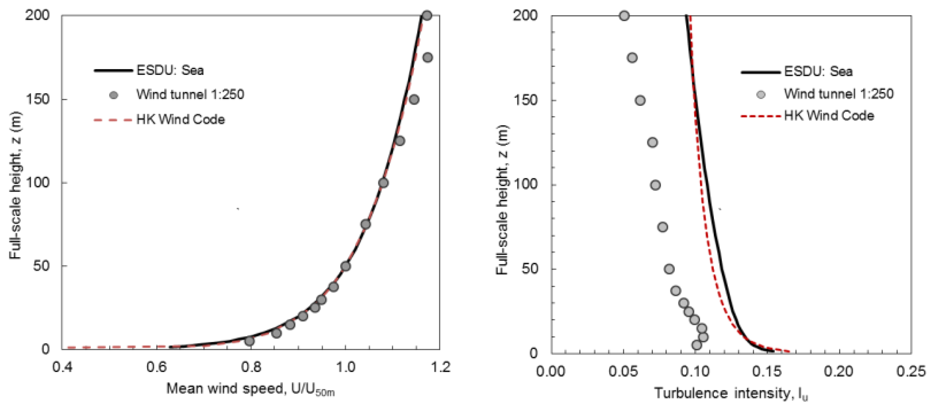
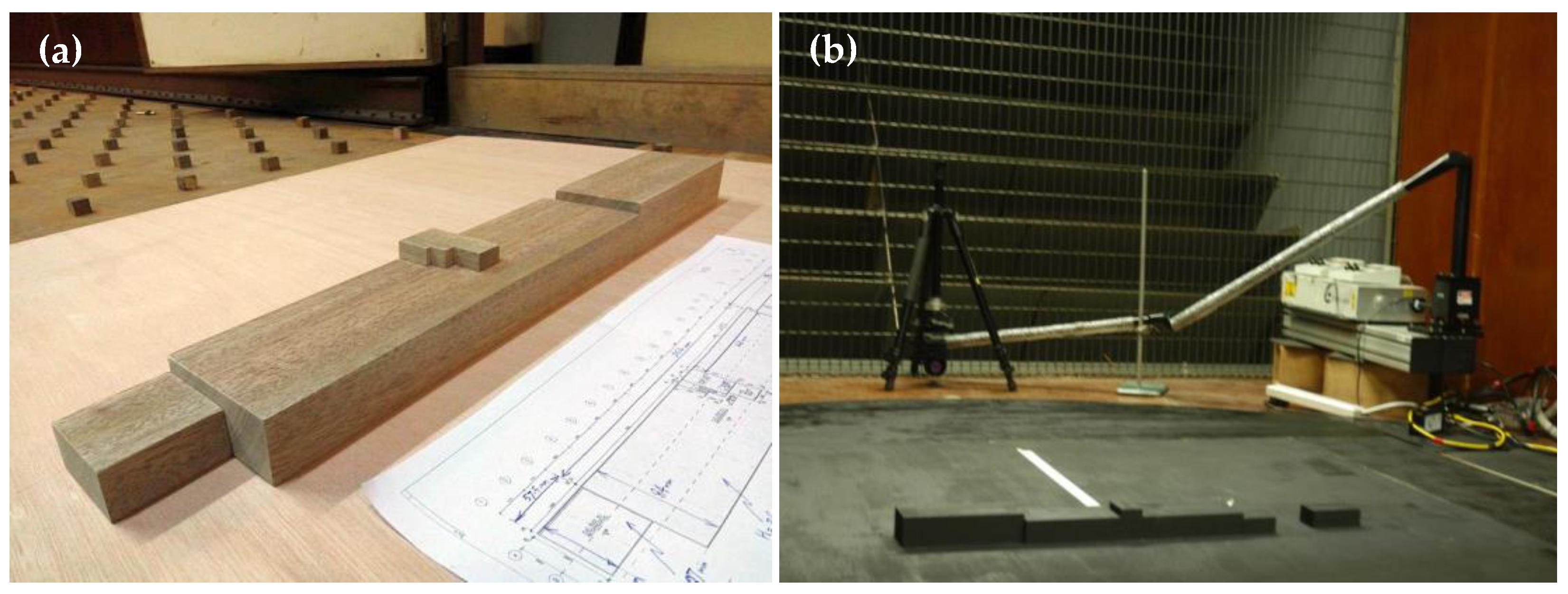
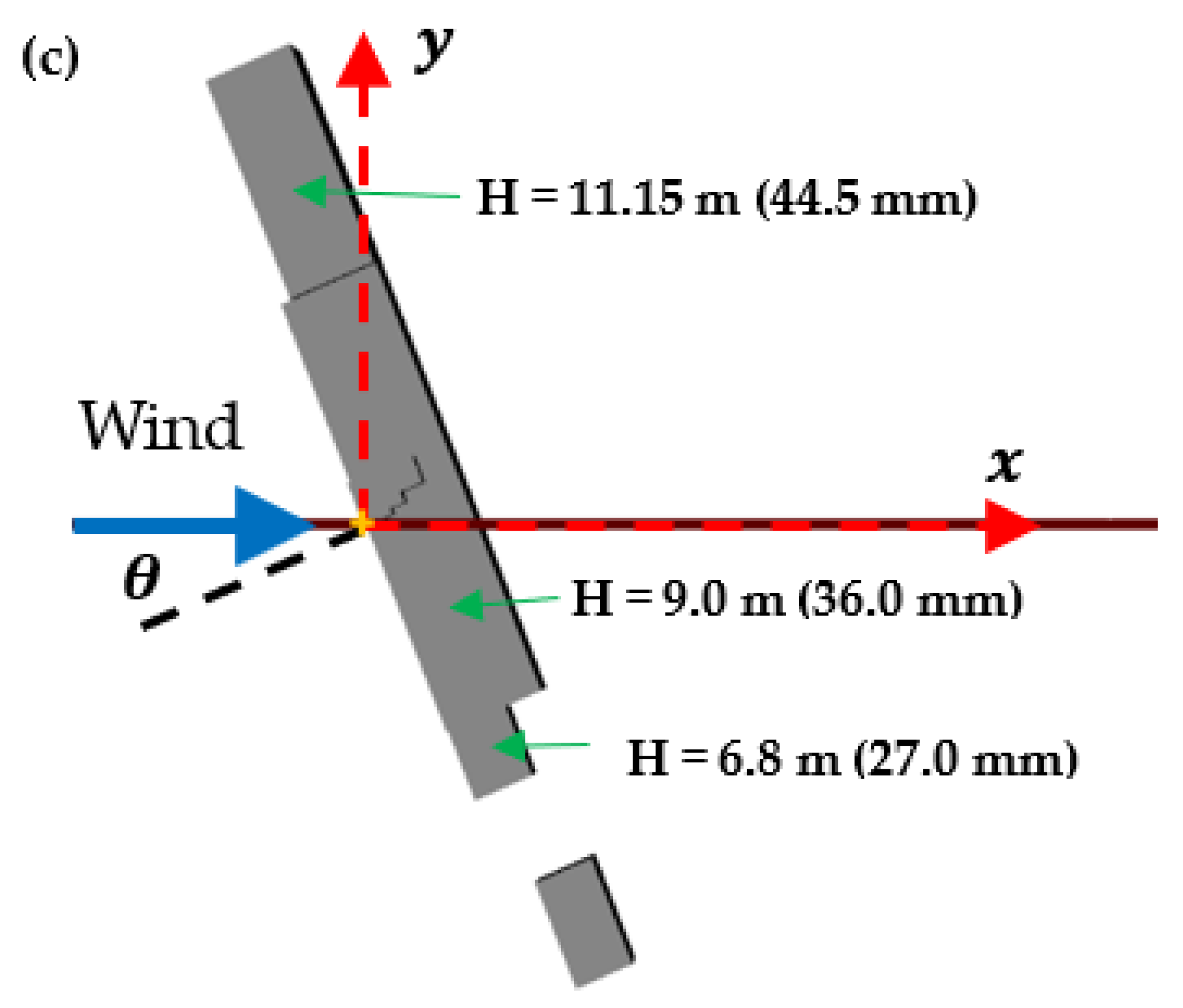
2.1. Wind Tunnel Experiments

The building structure investigated in the present study is a proposed new building in HKIA. The wind tunnel experiments were conducted in the atmospheric boundary layer wind tunnel of the Department of Civil Engineering, the University of Hong Kong. The tunnel was of the closed return type and the working section is 12 m long, 3 m wide and 1.8 m high. Natural wind of the open land terrain was simulated at the scale of 1:250 using a combination of triangular spires and fetch of roughness elements upwind of the turntable. Figure 1 shows the mean streamwise wind speed and turbulence intensity ($I_u={\mathsf{\sigma }}_u/U$) profiles measured at the center of the turntable. An arbitrary reference velocity ($U_{50\mathrm{m}} \approx 5.7 \mathrm{m}/\mathrm{s}$) at the height of 50 m full-scale (0.2 m in a wind tunnel) is chosen for normalization. The profiles of the Hong Kong Wind Code [31] and the ESDU profiles [32] for the open sea surface are also shown for comparison. The wind velocity profiles show a good agreement while the turbulence intensity values in the wind tunnel experiments are generally lower than those in the specifications as it is difficult to achieve high values near the ground at this geometry scale. The turbulence intensity at the height of the building model is about 0.10.

The down-scaled (1:250) model of the building was constructed by wood. Figure 2a shows a photograph of the building model. Besides the main building structure, there was a small structure to the south. The models were installed in the center of the turntable in the wind tunnel (Figure 2b). The model heights of the three rectangular parts of the main building structure were 27.0 mm, 36.0 mm and 44.5 mm, respectively, corresponding to the full-scale heights at 6.8 m, 9.0 m and 11.15 m (shown in Figure 2c). The height of the upper roof structure in the model was 47.5 mm above ground, which targeted a full-scale height of 12.2 m.

To simulate wind flow over buildings in the wind tunnel, a minimum value of Reynolds number ($Re$) needs to be achieved. Snyder [33] suggested that $Re$ should be greater than $1.1\times {10}^4$ to ensure independence, with $Re=U_{h}L/\mathsf{\nu }$. The scaling length L was calculated from the building face dimensions, corresponding to $104.5\mathrm{mm}$ or $54.9\mathrm{mm}$ for normal wind incidence on the longer or shorter side, respectively. Wind tunnel tests were carried out at mean wind speed $U_h\approx 5 \mathrm{m}/\mathrm{s}$ at the roof height of the model. With kinematic viscosity of air at $\mathsf{\nu }=1.54\times {10}^{-5} {\mathrm{m}}^2/\mathrm{s}$, the Reynolds number of wind tunnel testing was about $3.39\times {10}^4$ or $1.78\times {10}^4$, which satisfies the Re independence criterion mentioned above.

2.2. Particle Image Velocimetry (PIV) Measurement

The whole-field velocity measurement technique, particle image velocimetry (PIV), was applied to obtain the instantaneous flow information in the regions of interest (ROIs). The PIV system from Dantec Dynamics was used in this study. The measurement plane of physical size approximately 480 mm × 300 mm was illuminated by a thin laser sheet generated from the laser beam of a double-cavity Q-switched Nd:YAG laser (from Litron). The laser, laser sheet generator, and laser steering arm were placed inside the working section of the wind tunnel and located downstream of the turntable to avoid disturbing the flow field (Figure 2b). To minimize light reflection, the building models were painted black as well as the wind tunnel floor. Seeding particles of diameters at about 2 to 5 $\mathsf{\mu }\mathrm{m}$ were produced and introduced to the wind tunnel using a high-volume liquid seeding generator (10F03, Dantec Dynamics). Flow images were recorded by a sensitive high-speed CCD camera (SpeedSense M120, Dantec Dynamics). The camera had a high sensitivity for the weak scattered light in airflow and a resolution of 1920 × 1200 pixels. The camera framing speed was set at 100 double-image per second to capture a time sequence of particle images of length 500 double images.

The PIV analysis software used the spatial cross-correlation algorithm with adaptive and multi-pass interrogation windows. In the final iteration, PIV vectors were obtained on interrogation areas of size 32 × 32 pixels. The number of velocity vectors in each PIV snapshot was 60 × 37. The spatial resolution of the vectors was about 8 mm in the wind tunnel, that is, about 2 m in full scale. According to the study of Westerweel [34], the uncertainty of instantaneous velocity vectors was estimated to be $\Delta u/U_h\approx \pm 0.03$. In each measurement, the 500 PIV snapshots were captured for analysis.

Wake velocities were measured on the horizontal planes at 40 mm height (10 m full-scale). Hereafter, all the geometry lengths will be described in full-scale values. The free-field mean wind speed ($U_{ref}$) at this height, that is, without the building model, was about 4.8 m/s during the wind tunnel tests. The PIV measurement region was relatively small, corresponding to about 120 m × 75 m in full scale. To obtain more wake information, separate measurements were made at two different regions of interest (ROI-1 for near wake and ROI-2 for far wake). The specific locations of these two regions were marked in Figure 3b.

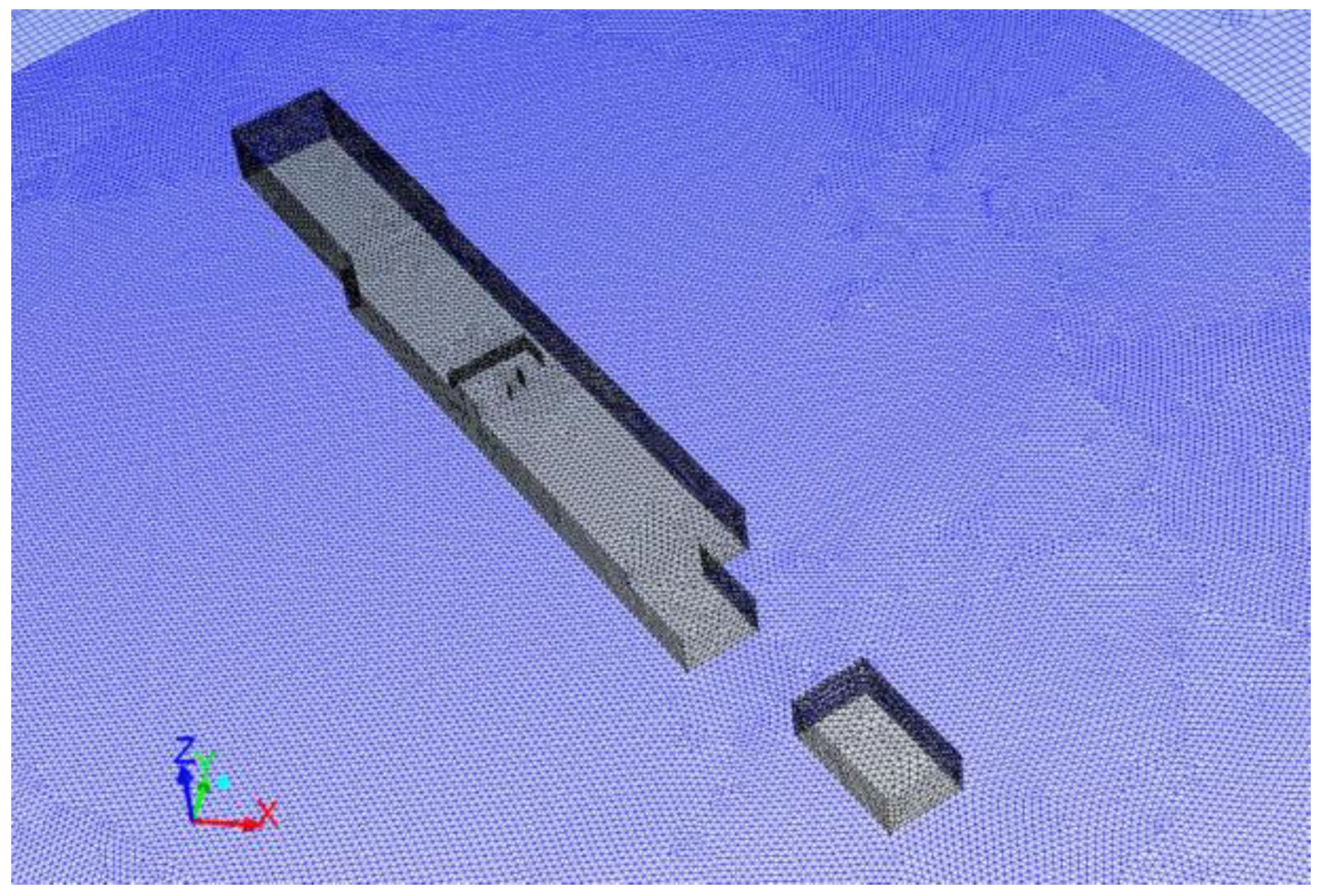
2.3. Computational Fluid Dynamics (CFD) Simulation

To obtain the flow field over a much larger region of the same building models, CFD studies were carried out to supplement the wind tunnel PIV measurements. In the full-scale sense, the building models were put inside a computation domain of height 250 m. The along-wind length of the domain was 1125 m covering $x\left(\mathrm{m}\right)\in \left[-200,925\right]$ and the lateral width is 600 m covering $y\left(\mathrm{m}\right)\in \left[-300,300\right]$, where the building center was set at the origin. More than 4 million cells were used to discretize the fluid space. The building surfaces were modeled with over 24,500 quadrilateral surface meshes (Figure 4). Along the smaller enveloping width of the building, there were at least 20 meshes. The bottom of the domain is the ground which was modeled by over 12,300 surface meshes.

The steady Reynolds-averaged Navier–Stokes (RANS) calculation equipped with realizable $k-\epsilon$ turbulence method was used to seek the time-averaged mean velocity field in this study. CFD computation was performed for the same wind angles as the wind tunnel tests, which included oblique wind incidence effects. Vertical profiles of mean wind speed and turbulence intensity as measured in the wind tunnel (Figure 1) were employed as the inlet boundary conditions. For other surfaces of the spatial domain, the top and sides were set as symmetry and the outlet was modeled with the pressure outlet condition. The ground and all building surfaces were treated as no-slip walls.

In the flow computation, the governing equations were solved numerically throughout the computational domain with the finite volume method (ANSYS Fluent). The computation was set to converge to a solution when the residuals of all computation variables fell below $1\times {10}^{-5}$. For the present cases, it took about $5000$ iterations to converge to a steady flow solution.

3. Results and Discussion

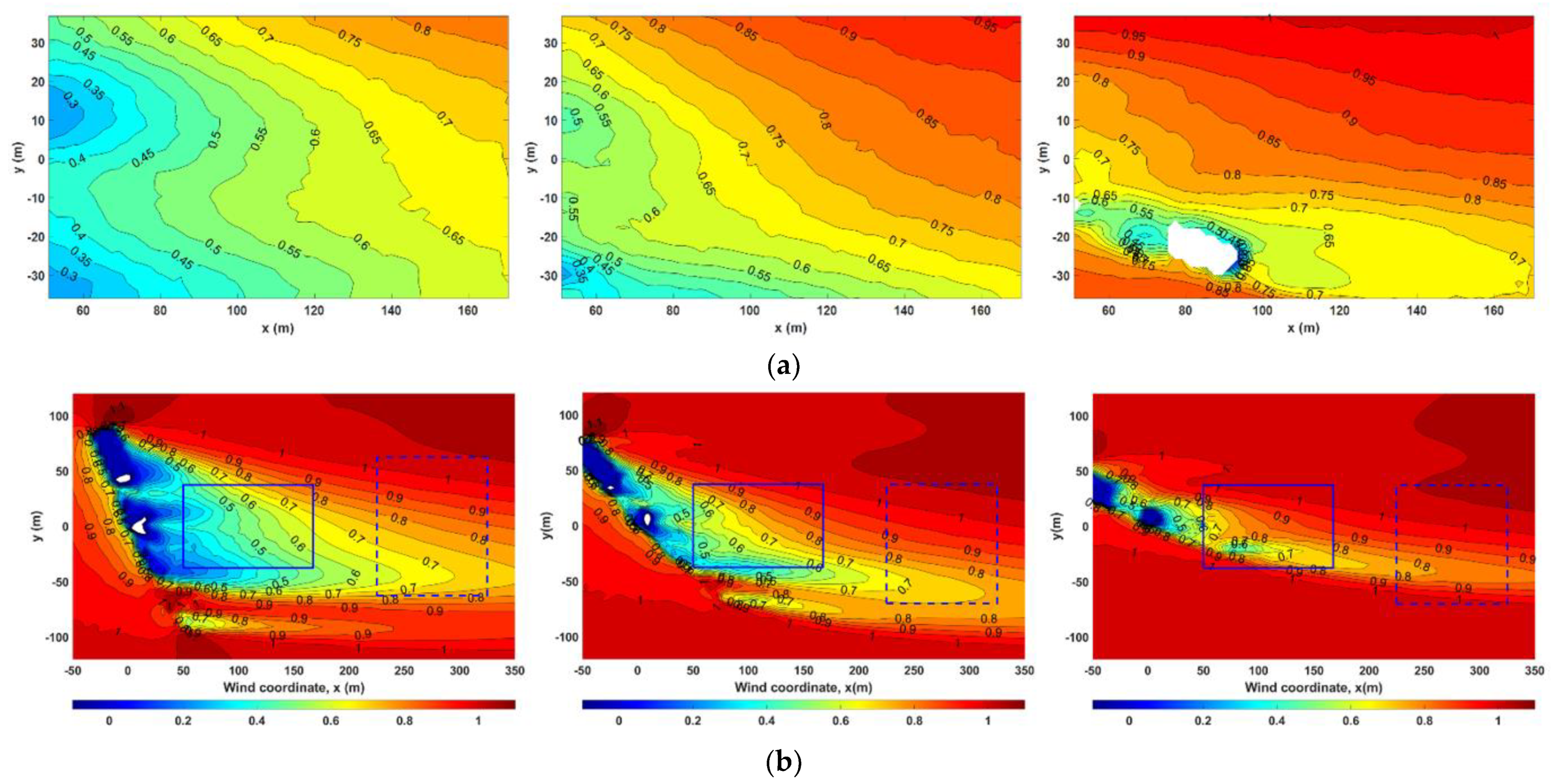
3.1. Three-Dimensional Mean Wake Deflection

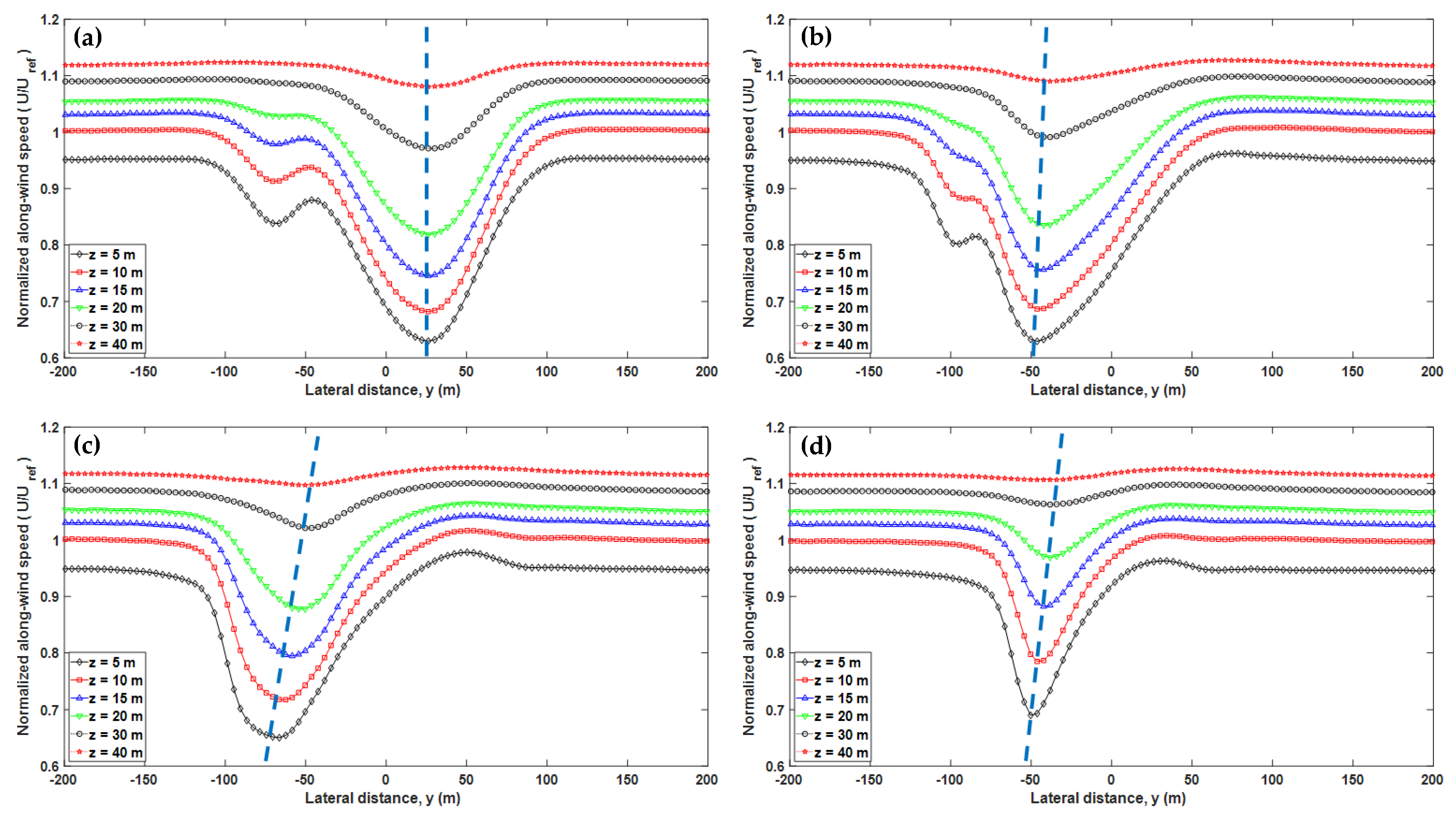
3.1.1. Mean Wake Deflection Phenomenon

The time-averaged mean along-wind velocity distributions in the far-wake (ROI-2) region behind the target model at three oblique incidences are displayed in Figure 5. These experimental PIV data are all normalized by the mean velocity of the free field (i.e., without building models). For the whole picture of the mean wake pattern, the CFD simulation results are illustrated in Figure 3. The PIV data in the near-wake (ROI-1) region are also shown for comparison. It is found that the mean wake characteristics of this elongated low-rise building obtained from the PIV measurements could be roughly captured by the RANS-based CFD computations, although the wake velocities obtained in CFD are slightly larger than those in wind tunnel experiments. Indeed, in terms of building wake estimation, the RANS calculation is generally considered not able to reproduce bluff body wake flow accurately. The building wake size is more likely to be overestimated [35,36].

When the building model is aligned at an oblique angle to the incoming wind, both PIV and CFD data support that the building wake, particularly the far-wake flow, tends to deflect towards the more downwind end of the building. It leads to a more severe asymmetry of the wake (hereafter referred to as the “wake deflection” phenomenon). In earlier studies on wind flow or sand erosion around low-rise buildings at oblique incidences, the characteristics and effects of wake deflection have not been explored quantitatively and explicitly [22,37]. Recently, the experimental work of Perry et al. [26] and numerical simulation of Foroutan et al. [27] are more relevant to this study by pointing out that the wake skewness could affect the pollutant dispersion process downstream. However, the limitation is that their results are mainly derived from the viewpoint of pollutant concentration distribution rather than the wind flow field itself. In essence, it is important to characterize the deflected wake flow directly, improving our understanding of the base flow structure at the oblique winds. More importantly, due to the three-dimensional feature of turbulent wake flow, more effort is required to characterize the deflection in detail.

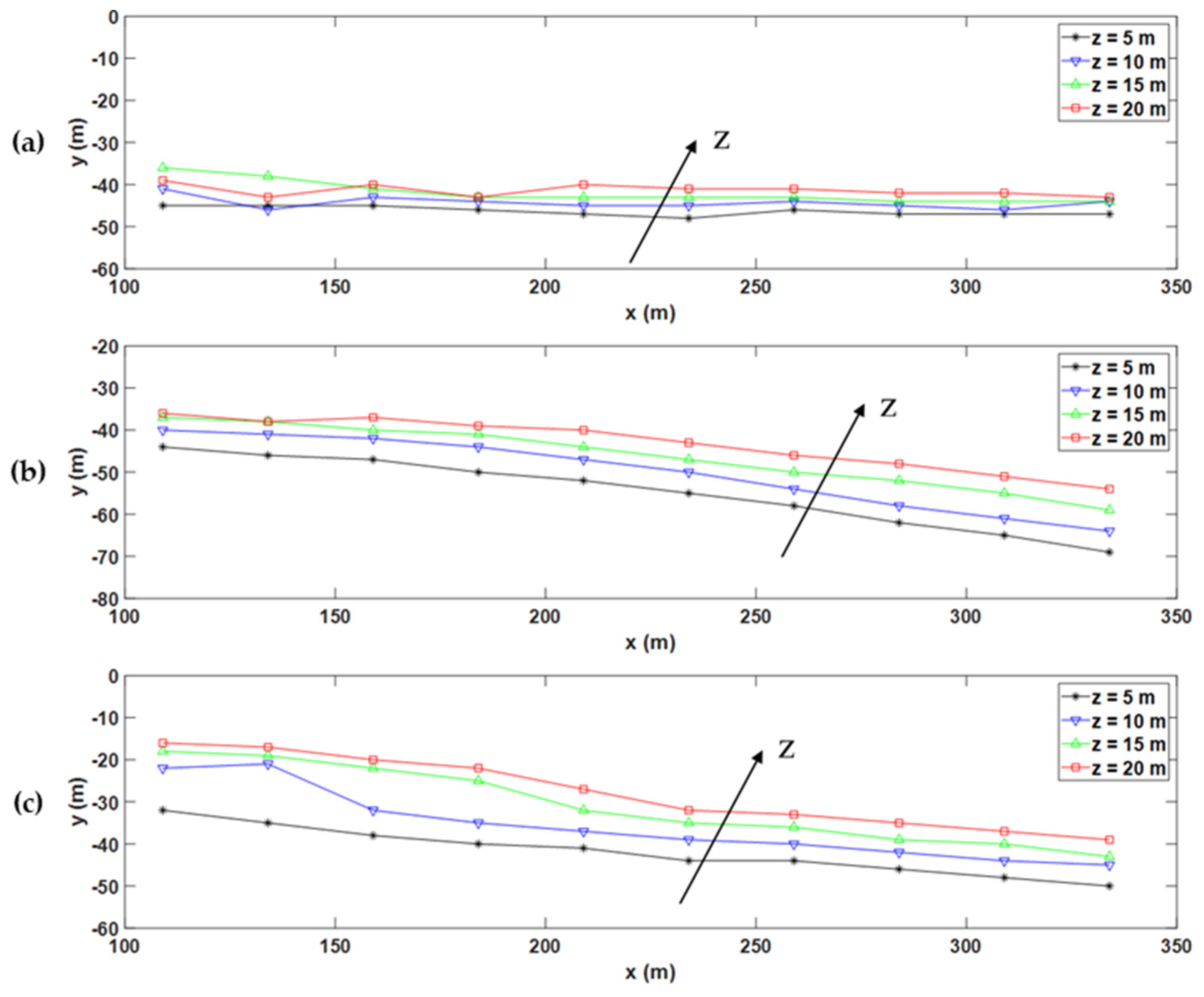
3.1.2. Streamwise Development of Lateral Wake Deflection

In Figure 6, the trajectories of maximum deficits of mean along-wind velocity at the height of 10 m are presented to describe the wake development. The locations of maximum velocity deficits are extracted from the lateral profiles of computed mean along-wind velocity, i.e., $\overline{U}\left(y\right)$, at successive streamwise x-stations. Similar to the observation from Figure 4 and Figure 5, the lateral deflection phenomenon is evidently observed and mainly occurs when the incident angle is equal to or greater than ${45}^{°}$ in terms of wake deflection angle. By comparison with the experimental data shown in Figure 4, it is promising to note that the deflection angles are in approximate agreement with those from the CFD data. In the case of ${22.5}^{°}$, the trajectory from the PIV data is almost parallel to the original prevailing wind direction. However, it is still observed that the wake is skewed and loses its symmetry.

In our proposition, there is a two-step mechanism determining the wake deflection and its extension in the wake from upstream to downstream: (1) the oblique wind incidence induced distortion of shear layer flow competition in the near-wake close to the downwind corner (hereafter referred to as “WD1”); and (2) the extended influence of deflected prevailing wind in the far-wake region (hereafter referred to as “WD2”). The present study only covers a few oblique wind incident angles but the evidence of wake flow deflection is revealed clearly and directly from Figure 6. Moreover, it is reasonable to infer the existence of a critical wind incident angle associating with the most deflected far-wake pattern, which is more likely to be around ${45}^{°}$ in this study case. For the symmetry-breaking variation of the near-wake pattern with the wind incidence, it is a bit too complex to draw some convincing conclusions in this study because of the presence of a small building downstream. However, at least, it is believed that there is another transition process from the symmetry case at $0^{°}$ to the downstream corner clustering pattern. Surely, these two critical states are both determined by many other influencing factors and it would be very interesting to quantify and estimate the wake deflection of an isolated building with different geometry shapes and under different boundary layer conditions in the future. In this study, we focus more on the far-wake deflection, covering $x\left(\mathrm{m}\right)\in \left[200,350\right]$, which means we can compare the effect of WD2 by the slope change of the trajectory. The effect of WD1 is assumed to be dominant within the nearer region (e.g., $x\le 150$ m), initializing the deflection induced by WD2. In this way, if we go back to Figure 6, it is concluded that the effect of WD1 is almost the same for the cases of ${22.5}^{°}$ and ${45}^{°}$ which is more significant than ${67.5}^{°}$ while the effect of WD2 reaches its maximum (estimated) at $\theta ={45}^{°}$. The small change of lateral deflection in the near-wake region at all three cases supports our assumption of WD1 properly.

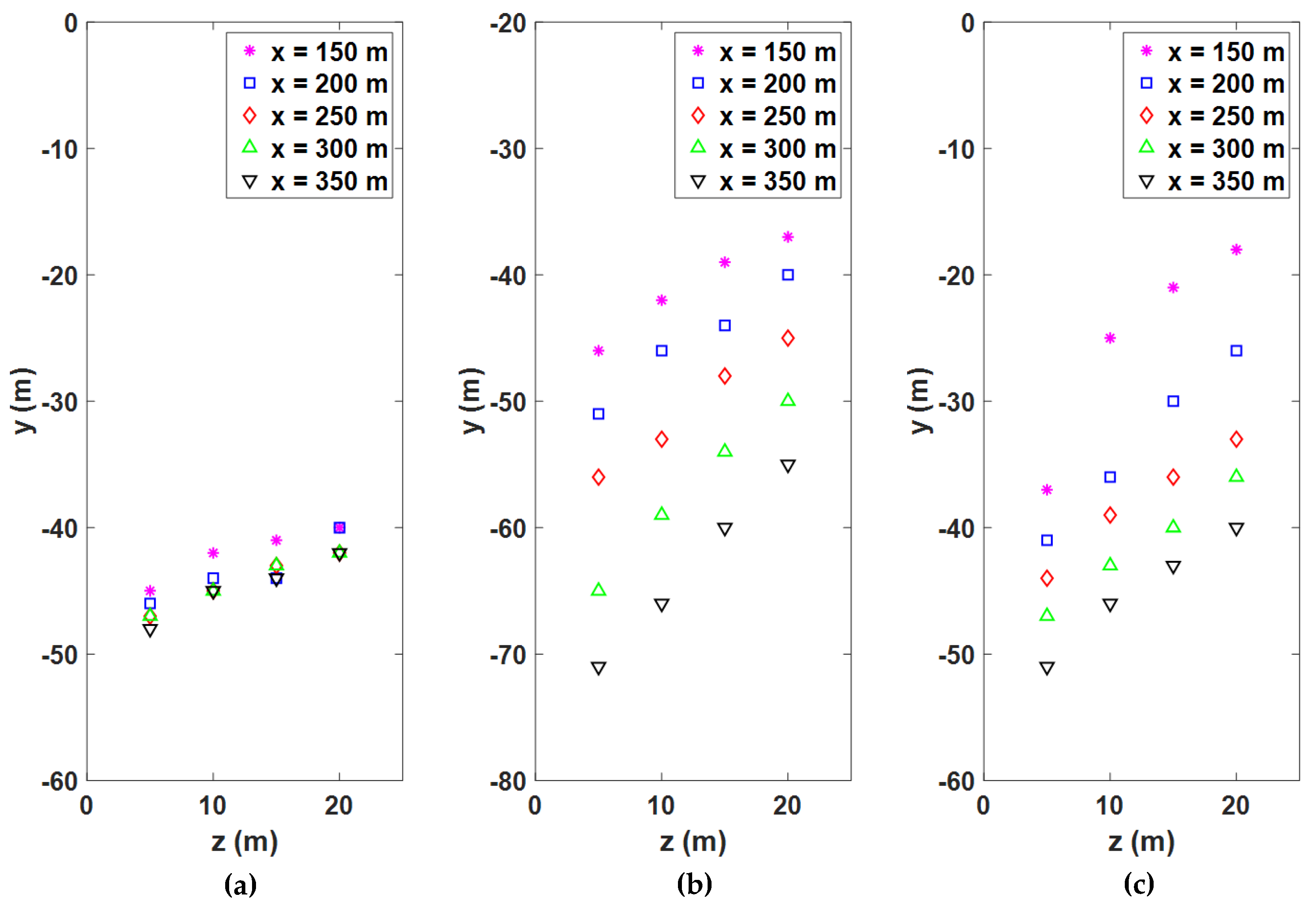
3.1.3. Vertical Variation of Lateral Wake Deflection

Aiming at a better understanding of the three-dimensional wake deflection, the streamwise development of maximum deficit trajectories at different heights is shown in Figure 7 with the help of CFD simulations. At $\theta ={22.5}^{°}$, the variation of trajectories is obviously less significant with the height than those at larger wind incidences. In general, the wake deflection due to WD1 will be weakened with the increasing height. To be more specific, as seen in Figure 7, the increase in height makes the trajectory curve shift towards the center line in the viewpoint of geometry distribution. Moreover, the WD2 induced wake deflection seems unchanged for each oblique wind incidence as the slope of the trajectory curve remains the same and nearly parallel with each other in the far-wake region. Interestingly, the increase in a lateral shift in the x-direction roughly follows the linear rule except in the case of ${67.5}^{°}$, which is slightly nonlinear. We cannot explain this result explicitly at the current stage as the interference effect of the downstream small building may play an important role.

To illustrate the variation of wake velocities at different heights, the lateral profiles of along-wind speed, $\overline{U}\left(y\right)$, at $x\approx 325\mathrm{m}$ are shown in Figure 8. Some of the observations made in the previous paragraph are further confirmed. The data at $\theta =0^{°}$ are also added for comparison. As expected, no wake deflection is observed although there is a lateral shift of the peaks which is due to the definition of the origin of the coordinate system. At oblique wind incidences, the lateral shift of maximum velocity deficits at different heights could be observed clearly. The most deflected wake is again confirmed at ${45}^{°}$. In order to unveil the linear characteristics of lateral wake deflection in the vertical direction, Figure 9 shows the variation of locations where maximum along-wind velocity deficits are detected. Remarkably, the linearity (or approximate) is broadly observed again in the far-wake region within the height of 20 m which is about two times the building height. Some weak nonlinearity occasionally appears, for instance, in the downstream region at $\theta ={67.5}^{°}$.

3.2. Aviation Risk Assessment

3.2.1. Verification of Existing Criteria

As depicted in Figure 4 and Figure 5, the wake velocity deficit in both PIV measurements and CFD simulations becomes weaker gradually with the downstream distance away from the building. Lateral profiles of $\overline{U}\left(y\right)$ at the downwind end of ROI-2 are shown in Figure 10. This is the most downstream location of the present PIV data (at full-scale target height of 10 m) and these are measured at a distance $x\approx 1350\mathrm{mm}$ behind the model, corresponding to about 337.5 m in full-scale from the building center. This distance roughly meets the requirement of the “1:35” construction criterion used by Amsterdam’s Schiphol Airport as most part of the test building is about 9 m in height.

Furthermore, the “7-knot” criterion advocated by Hong Kong Observatory (HKO) for the assessment of building wake effect on the aviation safety of aircraft upon landing and takeoff is also evaluated. For this purpose, the time-averaged along-wind velocity measurement data are scaled up to a background crosswind of 25 knots. In the present coordinate system, the along-wind velocity component directly represents the crosswind speed that appeared to an aircraft traveling on the runway (which is normal to the x-axis). It is evident from Figure 10 that the wake velocity variation along the lateral traverse does not violate the “7-knot” criterion at all wind incidence angles. The differences between the maximum and minimum time-averaged along-wind speeds at the four wind incidences are all below 6 knots.

In Figure 11, some instantaneous profiles of crosswind speed variation along the lateral direction at $\mathrm{x}\approx 337.5\mathrm{m}$ are presented for comparison to the time-averaged mean crosswind speed profile. It is clear that the instantaneous wake velocities fluctuate frequently and dramatically with time. The intense fluctuations at different wind incident angles all demonstrate that the “7-knot” criterion will be frequently violated if instantaneous wake velocities are used for evaluation. Therefore, a further estimation of exceedance probability over 7 knots is highly promoted due to the instantaneous velocity fluctuation.

3.2.2. Exceedance Probability Analysis

The ideas employed in this section to define the event of maximum velocity variations are explained in Figure 12 and Figure 13 as well as the corresponding analysis results. Two different scenarios are defined and discussed. Scenario A is mainly based on the assumption that the operation velocity of aircraft is extremely fast and thus the aircraft could experience all the instantaneous along-wind velocities within the region of interest. The event of maximum velocity difference is determined by each snapshot of PIV independently. As illustrated in Figure 12a, the maximum velocity difference is calculated and eventually, there are 500 events recorded in total. Figure 12b presented the probability distribution of these data of $\Delta U$, taking $\theta$ = ${22.5}^{°}$ as an example. In the frequency distribution histogram, the threshold value (7 knots) is marked to further estimate the exceedance probability (Pr($\Delta U\ge 7$)). The reliability of the “7-knot” criterion is evaluated by displaying the exceedance probability at different wind incident angles in Figure 12c. With the fluctuating component considered, it is clear that the “7-knot” criterion is not suitable for the instantaneous wake effect. The exceedance probabilities are all greater than 75%.

In Scenario B, the practical operation speed of aircraft is considered. The inclusion of velocity variations at different time instants and spatial locations makes the assessment more robust and reliable. According to the scale factor adopted in the wind tunnel experiments, the sampling frequency of 100 Hz represents a time interval of 1 sec between successive flow realizations. The lateral distance under observation is about 100 m in full scale. Thus, the maximum resolvable aircraft velocity is about 100 m/s (or 194 knots) which means if the aircraft running through the observing region with a speed larger than this value will directly lead to information distortion and loss. In practice, the take-off and landing speed of aircraft usually depends on many factors, such as wind conditions, the weight of aircraft, ambient temperature/humidity, airport elevation, and degree of flaps, etc. For an average-sized commercial jetliner with typical fuel and payload, the take-off speed is around 130–200 knots while the landing speed is more or less the same, normally a few knots slower. Without loss of generality, a compromised value of 165 knots (85 m/s) is selected as a typical aircraft take-off (or landing) speed which slightly exceeds the landing speed of Boeing 747 of about 150 knots. Due to the limitation of experimental devices, only the time interval $\Delta T$ = 1 s is available for analysis, corresponding to a movement of 85 m. Meanwhile, the concept of “in a short time interval” is thus specified. As illustrated in Figure 13a, the velocity differences $\Delta U_i$ are collected by identifying the maximum difference ($\Delta U_{max}=\max \left\{\Delta U_i\right\}$) between each two neighbored datasets which are recognized as the most unfavorable extreme event experienced by the aircraft for each trial. Consequently, 499 trials are performed altogether to estimate the exceeding probability over 7 knots at different wind incident angles. Similar to the exceedance probability analysis procedure presented in Scenario A, the exceedance probabilities in Scenario B are shown in Figure 13b. As expected, the exceedance probability decreases significantly compared with the results in Figure 12c. However, it should be noted that there is still a 50% probability of breaking the criterion. Therefore, the importance of velocity fluctuation in the building wake on aviation safety assessment should be emphasized in the future.

4. Concluding Remarks

In this paper, the turbulent wake flow of an elongated low-rise building is analyzed with the aid of experimental PIV measurements and RANS-based CFD simulations. Two important issues, i.e., the mean wake deflection and aviation safety assessment, are discussed. The major conclusions are summarized below.

The lateral mean wake deflection phenomenon is clearly revealed at oblique wind incidences. For quantitative description, a two-step mechanism is proposed to understand the wake deflection process and its evolution in the wake. The oblique wind incidence leads to a distortion of shear layer flow competition in the near-wake region (WD1) and then the deflected prevailing wind extends its effect in the far-wake region (WD2). The WD1 effect provides an initial state for the development of WD2 and the effect of WD2 is mainly characterized by the slope angle of trajectory of maximum wake velocity deficit representing the wake pattern development. For CFD simulation, although RANS was shown to overestimate the wake size, the WD2 effect in the far-wake region agrees reasonably well with the PIV measurements. The numerical simulations showing the variation of lateral wake deflection change in space promote our understanding of the three-dimensional wake structure. In the streamwise direction, it is found that the effect of WD1 is almost the same for the cases of ${22.5}^{°}$ and ${45}^{°}$, which is more significant than ${67.5}^{°}$, while the effect of WD2 reaches its maximum (estimated) at $\theta ={45}^{°}$. In the vertical direction, the increase in height weakens the WD1-induced deflection but plays an insignificant role in the WD2 effect. More interestingly, in both the streamwise and vertical directions, the WD2 effect shows a good linearity feature within the region of interest.

From the wake of the particular building located in an airport, the assessment of its building wake effect using existing mean wake-based aviation safety assessment criteria, “1:35 rule” and “7-knot criterion”, is discussed. At the selected downstream location at about 35 times the building height ($x\approx 337.5\mathrm{m}$), both criteria show that the wake effect is marginally acceptable. However, by considering the fluctuating wake velocity component, the exceedance probability analysis points out the limitation of these two criteria explicitly. It may be needed to develop new evaluation methods in the future.

References

1. Mizota, T.; Okajima, A. Experimental studies of time mean flows around rectangular prisms. In Proceedings of the Japan Society of Civil Engineers; Japan Society of Civil Engineers: Tokyo, Japan, 1981; Volume 312, pp. 39–47. [Google Scholar]
2. Okajima, A. Strouhal numbers of rectangular cylinders. J. Fluid Mech. 1982, 123, 379–398. [Google Scholar] [CrossRef] [Green Version]
3. Sakamoto, H.; Arie, M. Vortex shedding from a rectangular prism and a circular cylinder placed vertically in a turbulent boundary layer. J. Fluid Mech. 1983, 126, 147–165. [Google Scholar] [CrossRef]
4. Sakamoto, H.; Oiwake, S. Fluctuating Forces on a Rectangular Prism and a Circular Cylinder Placed Vertically in a Turbulent Boundary Layer. J. Fluids Eng. 1984, 106, 160–166. [Google Scholar] [CrossRef]
5. Wang, H.F.; Zhou, Y. The finite-length square cylinder near wake. J. Fluid Mech. 2009, 638, 453–490. [Google Scholar] [CrossRef] [Green Version]
6. Sattari, P.; Bourgeois, J.A.; Martinuzzi, R.J. On the vortex dynamics in the wake of a finite surface-mounted square cylinder. Exp. Fluids 2012, 52, 1149–1167. [Google Scholar] [CrossRef]
7. Sumner, D.; Rostamy, N.; Bergstrom, D.; Bugg, J. Influence of aspect ratio on the mean flow field of a surface-mounted finite-height square prism. Int. J. Heat Fluid Flow 2017, 65, 1–20. [Google Scholar] [CrossRef]
8. Wang, F.; Lam, K.M. Geometry effects on mean wake topology and large-scale coherent structures of wall-mounted prisms. Phys. Fluids 2019, 31, 125109. [Google Scholar] [CrossRef]
9. Igarashi, T. Characteristics of the Flow around a Square Prism. Bull. JSME 1984, 27, 1858–1865. [Google Scholar] [CrossRef]
10. Huang, R.F.; Lin, B.H.; Yen, S.C. Time-averaged topological flow patterns and their influence on vortex shedding of a square cylinder in crossflow at incidence. J. Fluids Struct. 2010, 26, 406–429. [Google Scholar] [CrossRef]
11. Yen, S.C.; Yang, C.W. Flow patterns and vortex shedding behavior behind a square cylinder. J. Wind. Eng. Ind. Aerodyn. 2011, 99, 868–878. [Google Scholar] [CrossRef]
12. Unnikrishnan, S.; Ogunremi, A.; Sumner, D. The effect of incidence angle on the mean wake of surface-mounted finite-height square prisms. Int. J. Heat Fluid Flow 2017, 66, 137–156. [Google Scholar] [CrossRef]
13. Bourgeois, J.A.; Sattari, P.; Martinuzzi, R.J. Alternating half-loop shedding in the turbulent wake of a finite surface-mounted square cylinder with a thin boundary layer. Phys. Fluids 2011, 23, 095101. [Google Scholar] [CrossRef]
14. Castro, I.P.; Robins, A.G. The flow around a surface-mounted cube in uniform and turbulent streams. J. Fluid Mech. 1977, 79, 307–335. [Google Scholar] [CrossRef]
15. Hillier, R.; Cherry, N.J. The effects of stream turbulence on separation bubbles. J. Wind. Eng. Ind. Aerodyn. 1981, 8, 49–58. [Google Scholar] [CrossRef]
16. Ballio, F.; Bettoni, C.; Franzetti, S. A Survey of Time-Averaged Characteristics of Laminar and Turbulent Horseshoe Vortices. J. Fluids Eng. 1998, 120, 233–242. [Google Scholar] [CrossRef]
17. Wang, H.F.; Zhou, Y.; Chan, C.K.; Lam, K.S. Effect of initial conditions on interaction between a boundary layer and a wall-mounted finite-length-cylinder wake. Phys. Fluids 2006, 18, 065106. [Google Scholar] [CrossRef] [Green Version]
18. Hosseini, Z.; Bourgeois, J.A.; Martinuzzi, R.J. Large-scale structures in dipole and quadrupole wakes of a wall-mounted finite rectangular cylinder. Exp. Fluids 2013, 54, 1595. [Google Scholar] [CrossRef]
19. Li, Q.S.; Hu, G.; Yan, B.-W. Investigation of the effects of free-stream turbulence on wind-induced responses of tall building by Large Eddy Simulation. Wind. Struct. Int. J. 2014, 18, 599–618. [Google Scholar] [CrossRef]
20. El Hassan, M.; Bourgeois, J.; Martinuzzi, R. Boundary layer effect on the vortex shedding of wall-mounted rectangular cylinder. Exp. Fluids 2015, 56, 33. [Google Scholar] [CrossRef]
21. Hearst, R.J.; Gomit, G.; Ganapathisubramani, B. Database—Effect of turbulence on the wake of a wall-mounted cube. J. Fluid Mech. 2016, 804, 513–530. [Google Scholar] [CrossRef]
22. Blocken, B.B.; Carmeliet, J. Pedestrian Wind Environment around Buildings: Literature Review and Practical Examples. J. Therm. Envel. Build. Sci. 2004, 28, 107–159. [Google Scholar] [CrossRef]
23. Blocken, B.; Carmeliet, J. Pedestrian wind conditions at outdoor platforms in a high-rise apartment building: Generic sub-configuration validation, wind comfort assessment and uncertainty issues. Wind. Struct. Int. J. 2008, 11, 51–70. [Google Scholar] [CrossRef] [Green Version]
24. Blocken, B. 50 years of computational wind engineering: Past, present and future. J. Wind. Eng. Ind. Aerodyn. 2014, 129, 69–102. [Google Scholar] [CrossRef]
25. Zargar, A.; Gungor, A.; Tarokh, A.; Hemmati, A. Coherent structures in the wake of a long wall-mounted rectangular prism at large incident angles. Phys. Rev. Fluids 2021, 6, 034603. [Google Scholar] [CrossRef]
26. Perry, S.; Heist, D.; Brouwer, L.; Monbureau, E.; Brixey, L. Characterization of pollutant dispersion near elongated buildings based on wind tunnel simulations. Atmos. Environ. 2016, 142, 286–295. [Google Scholar] [CrossRef]
27. Foroutan, H.; Tang, W.; Heist, D.; Perry, S.; Brouwer, L.; Monbureau, E. Numerical analysis of pollutant dispersion around elongated buildings: An embedded large eddy simulation approach. Atmos. Environ. 2018, 187, 117–130. [Google Scholar] [CrossRef] [PubMed]
28. Krüs, H.; Haanstra, J.; Van Der Ham, R.; Schreur, B. Numerical simulations of wind measurements at Amsterdam Airport Schiphol. J. Wind. Eng. Ind. Aerodyn. 2003, 91, 1215–1223. [Google Scholar] [CrossRef]
29. Hong Kong Observatory (HKO). Low Level Wind Effect at Airports—Information for Pilots and Planners of New Buildings. HKP Pamphlet (2012). Available online: https://www.hko.gov.hk/en/aviat/articles/files/llw_pamphlet_3col_v17.pdf (accessed on 7 May 2021).
30. Nieuwpoort, A.M.H.; Gooden, J.H.M.; de Prins, J.L. Wind Criteria due to Obstacles at and around Airports; NLR-CR-2006-261; National Aerospace Laboratory: Bengaluru, India, 2010; 200p. [Google Scholar]
31. HKBD (Hong Kong Buildings Department). Code of Practice on Wind Effects in Hong Kong 2004; Institution of Structural Engineers: Hong Kong, China, 2004. [Google Scholar]
32. ESDU (Engineering Sciences Data Unit). Strong Winds in the Atmospheric Boundary Layer; Part 1: Hourly Mean Wind Speeds; Data Item 82026; ESDU: London, UK, 2002. [Google Scholar]
33. Snyder, W.H. Guideline for Fluid Modeling of Atmospheric Diffusion; Environmental Sciences Research Laboratory, Office of Research and Development, US Environmental Protection Agency: Washington, DC, USA, 1981; Volume 81. [Google Scholar]
34. Westerweel, J. Theoretical analysis of the measurement precision in particle image velocimetry. Exp. Fluids 2000, 29, S003–S012. [Google Scholar] [CrossRef]
35. Tominaga, Y. Flow around a high-rise building using steady and unsteady RANS CFD: Effect of large-scale fluctuations on the velocity statistics. J. Wind. Eng. Ind. Aerodyn. 2015, 142, 93–103. [Google Scholar] [CrossRef]
36. Lin, C.; Ooka, R.; Kikumoto, H.; Sato, T.; Arai, M. CFD simulations on high-buoyancy gas dispersion in the wake of an isolated cubic building using steady RANS model and LES. Build. Environ. 2021, 188, 107478. [Google Scholar] [CrossRef]
37. Becker, S.; Lienhart, H.; Durst, F. Flow around three-dimensional obstacles in boundary layers. J. Wind. Eng. Ind. Aerodyn. 2002, 90, 265–279. [Google Scholar] [CrossRef]
Figure 1. Vertical profiles of mean wind speed and longitudinal turbulence intensity simulated in wind tunnel.
Atmosphere 12 01579 g001
Figure 2. (a) Experimental model of the building; (b) Layout in wind tunnel; (c) Heights, wind incidence and Cartesian coordinate system definition (“+” denotes origin point).
Atmosphere 12 01579 g002aAtmosphere 12 01579 g002b
Figure 3. Contours of U / U r e f at the height of 10 m (a) PIV measurements in the near-wake (ROI-1) region; (b) RANS-based CFD simulation results. (Left column: 22.5 ° ; middle column: 45 ° ; right column: 67.5 ° . The solid line marks the ROI-1 region while the dashed line defines the ROI-2 region).
Atmosphere 12 01579 g003
Figure 4. Surface meshes of buildings near ground in CFD model.
Atmosphere 12 01579 g004
Figure 5. Contours of U / U r e f in the far-wake (ROI-2) region at the height of 10 m: (a) 22.5 ° ; (b) 45 ° ; (c) 67.5 ° .
Atmosphere 12 01579 g005
Figure 6. Trajectories of maximum deficit of mean along-wind velocity in the lateral direction at the height of 10 m.
Atmosphere 12 01579 g006
Figure 7. Trajectories of maximum deficit of mean along-wind velocity in the lateral direction at different heights: (a) 22.5 ° ; (b) 45 ° ; (c) 67.5 ° .
Atmosphere 12 01579 g007
Figure 8. Lateral recovery of normalized along-wind speed at x   325   m : (a) 0 ° ; (b) 22.5 ° ; (c) 45 ° ; (d) 67.5 ° .
Atmosphere 12 01579 g008
Figure 9. Variation of maximum along-wind velocity deficits in the vertical direction: (a) 22.5 ° ; (b) 45 ° ; (c) 67.5 ° .
Atmosphere 12 01579 g009
Figure 10. Changes of time-averaged along-wind speed lateral traverse at x   337.5   m . Background wind speed ( U b ) is set as 25 knots.
Atmosphere 12 01579 g010
Figure 11. Instantaneous along-wind velocities: (a) 0 ° ; (b) 22.5 ° ; (c) 45 ° ; (d) 67.5 ° .
Atmosphere 12 01579 g011
Figure 12. Scenario A: (a) maximum velocity difference calculation; (b) Probability distribution of maximum velocity difference at wind angle 22.5 ° ; (c) Exceedance probability (Pr( Δ U 7 )) at different wind angles.
Atmosphere 12 01579 g012
Figure 13. Scenario B: (a) maximum velocity difference calculation under a pre-specified time interval (1 s) and aircraft operation speed (85 m/s); (b) Exceedance probability at different wind angles.
Atmosphere 12 01579 g013
Publisher’s Note: MDPI stays neutral with regard to jurisdictional claims in published maps and institutional affiliations.