Article

Fine and Coarse Carbonaceous Aerosol in Houston, TX, during DISCOVER-AQ

1
Department of Earth and Atmospheric Sciences, University of Houston, Houston, TX 77004, USA
2
Department of Environmental Science, Baylor University, Waco, TX 76706, USA
3
Department of Chemistry and Biochemistry, Baylor University, Waco, TX 76706, USA
*
Author to whom correspondence should be addressed.
Atmosphere 2020, 11(5), 482; https://doi.org/10.3390/atmos11050482
Submission received: 14 April 2020 / Revised: 5 May 2020 / Accepted: 7 May 2020 / Published: 9 May 2020
(This article belongs to the Special Issue Sources and Composition of Ambient Particulate Matter)

Abstract

:
To investigate major sources and trends of particulate pollution in Houston, total suspended particulate (TSP) and fine particulate matter (PM2.5) samples were collected and analyzed. Characterization of organic (OC) and elemental (EC) carbon combined with realtime black carbon (BC) concentration provided insight into the temporal trends of PM2.5 and coarse PM (subtraction of PM2.5 from TSP) during the Deriving Information on Surface Conditions from Column and VERtically Resolved Observations Relevant to Air Quality (DISCOVER-AQ) Campaign in Houston in 2013. Ambient OC, EC, and BC concentrations were highest in the morning, likely due to motor vehicle exhaust emissions associated with the morning rush hour. The morning periods also had the lowest OC to EC ratios, indicative of primary combustion sources. Houston also had significant coarse EC at the downtown site, with an average (±standard deviation) PM2.5 to TSP ratio of 0.52 ± 0.18 and an average coarse EC concentration of 0.44 ± 0.24 µg·C·m−3. The coarse EC concentrations were likely associated with less efficient industrial combustion processes from industry near downtown Houston. During the last week (20–28 September, 2013), increases in OC and EC concentrations were predominantly in the fine fraction. Both PM2.5 and TSP samples from the last week were further analyzed using radiocarbon analysis. Houston’s carbonaceous aerosol was determined to be largely from contemporary sources for both size fractions; however, PM2.5 had less impact from fossil sources. There was an increasing trend in fossil carbon during a period with the highest carbonaceous aerosol concentrations (September 24 night and 25 day) that was observed in both the PM2.5 and TSP. Overall, this study provided insight into the sources and trends of both fine and coarse PM in a large urban U.S. city impacted by a combination of urban, industrial, and biogenic emissions sources.

1. Introduction

It is important to improve characterization of carbonaceous aerosols because they impact both human health and global climate. Carbonaceous aerosols can impact climate change directly via absorption and scattering of radiation [1], as well as indirectly due to the aerosols’ ability to act as cloud condensation nuclei [2,3]. The complex interactions between carbonaceous aerosols and climate change are still being studied [4,5]. Similarly, the human health impacts of atmospheric aerosols are being investigated in urban settings. Prolonged exposure to respirable PM (PM10; particulates with an aerodynamic diameter of 10 µm and smaller), and more significantly fine PM (PM2.5; particulates with an aerodynamic diameter of 2.5 µm and smaller), has been found to cause respiratory and cardiopulmonary diseases and overall increased mortality [6,7,8]. In the short term, epidemiological studies have observed an increase in nonaccidental, respiratory-related hospital emergency visits on days with enhanced PM [9,10]. Thus, improving understanding of the sources and trends in urban aerosol will enable better mitigation strategies for both climate and human health.
Houston, TX, is the fourth most populous city in the U.S., with 2.3 million residents [11], and has an abundance of anthropogenic and natural emissions. The city’s air quality is impacted by urban emissions (e.g., motor vehicle exhaust (MVE), cooking, residential wood burning, etc.) and industrial emissions associated with activities in and around the Houston Ship Channel (HSC) (e.g., heavy-duty diesel exhaust, ship emissions, petrochemical and refinery processes, etc.) [12,13,14,15]. Houston, like many southeastern U.S. cities, is also heavily impacted by biogenic emissions from vegetation within the city and forested regions surrounding the city (e.g., Piney Woods) (Figure 1) [16,17,18]. The objective of this study was to chemically characterize Houston’s carbonaceous aerosol in the fine and coarse PM (PMTSP-2.5; subtraction of carbon concentration of PM2.5 from TSP) fractions to better understand the major sources and trends of PM in the city. For this study, filter samples and measurements were taken during the NASA-sponsored Deriving Information on Surface Conditions from Column and VERtically Resolved Observations Relevant to Air Quality (DISCOVER-AQ) campaign in September 2013 [19]. The purpose of the DISCOVER-AQ campaign was to use ground and airborne measurements to improve the efficiency of satellites in diagnosing ground-level air quality. This study focused on ground-based measurements and sampling at two sites: a primary urban site located near the downtown area, representative of the urban Houston region, while the auxiliary site located southeast of the city was near Trinity Bay and the HSC (Figure 1) [13,15]. Organic and elemental carbon (OC and EC, respectively) concentrations and radiocarbon (14C) analysis of the total carbon (TC: OC + EC) were used to characterize the carbonaceous aerosols. From these measurements, week 4 of the campaign (21–28 September), was designated as the week of interest due to the increased TC concentration in both the PM2.5 and TSP. Previous studies also observed increased PM2.5 mass and a peak ozone event across the Houston metropolitan area during week 4 [20,21,22]. In addition to these off-line analyses, real-time measurement of black carbon (BC) was made during this sampling period to evaluate hourly BC trends and compare to filter-based EC measurements. Though BC and EC are both used to describe the refractory fraction of carbonaceous aerosols, BC is defined by the aerosol’s optical attenuation [23], while EC is measured based on a thermal-optical approach [24]. More recent aerosol studies in Houston have focused on fine and submicron PM size fractions; however, this study provides an in-depth characterization of both fine and coarse carbonaceous aerosols in Houston in order to identify sources, trends, and relationships between these PM size fractions.

2. Methods and Materials
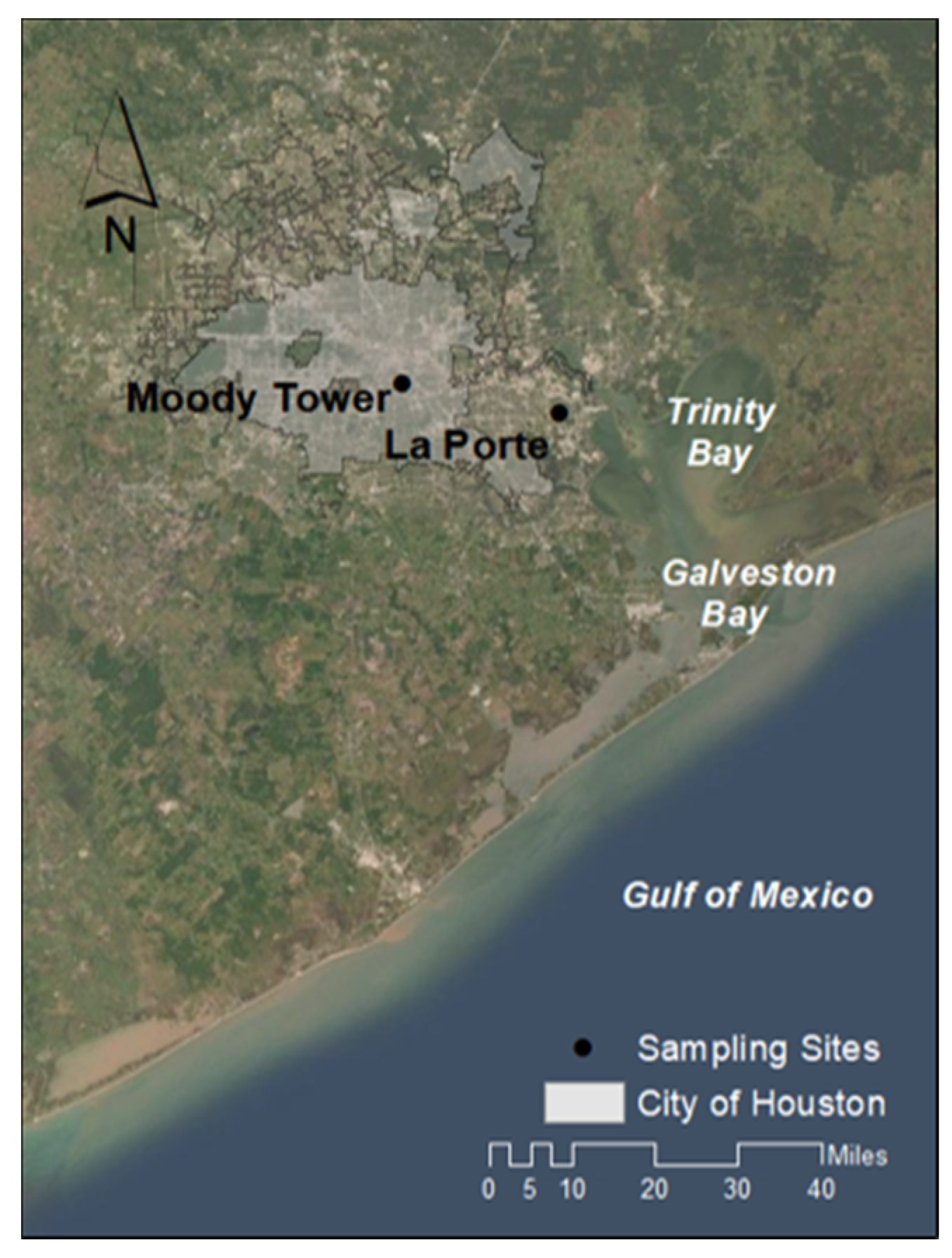
2.1. Sampling

PM filter-sample collection and BC measurement took place from 4 to 28 September and 1 to 30 September 2013, respectively. This sampling campaign was part of the larger DISCOVER-AQ campaign in Houston. The primary sampling site was on top of Moody Tower (MT; 29.7197, −95.3432), a high-rise residence hall (~70 m) located on the University of Houston’s campus. This site is approximately 4.4 km southeast of downtown Houston and northwest of the HSC (Figure 1). The auxiliary sampling site, La Porte (LP; 29.6721, −95.0647), was located within a small municipal airport approximately 5.6 km west of Trinity Bay and close to the HSC (Figure 1). The LP site provides spatial comparison to the primary urban site (MT), providing insight into whether trends observed at the urban core were present in other parts of the metropolitan area. The LP site is close to Trinity Bay and closer to the Gulf of Mexico, serving as potential upwind site for marine onshore winds to MT (Figure 1). This LP site is also in close proximity to the highly industrialized region of Houston (i.e., HSC).
During the campaign, PM2.5 samples were collected at MT, while TSP samples were collected at MT and LP. A Tisch sampler with a PM2.5 inlet (200 L·min−1, Tisch Environmental Inc. Cleves, OH, USA) and a URG medium-volume sampler with a PM2.5 cyclone (82 L·m−1, URG Corporation, Chapel Hill, NC, USA) were used for PM2.5 sample collection at MT. Two Tisch high-volume samplers (1170 and 1130 L·m−1) were alternated for TSP sample collection at MT. A Tisch high-volume sampler (1000 L·m−1) was also used for TSP sample collection at LP. The PM2.5 filter-sample collections at MT included morning (06:30 to 10:00), afternoon (10:00 to 20:00), day (06:30 to 20:00), and 24-h (06:30 to 06:00) samples (Table 1). The TSP filter-sample collections at MT included day and night (20:00 to 06:30) samples. The TSP filter-sample collection at LP included 24-h samples (Table 1). Both filter samples and blanks were collected on 90 mm and 102 mm quartz fiber filters for PM2.5 samples, respectively, while 20 × 25 cm quartz fiber filters were used for the TSP samples. All quartz fiber filters were pre-cleaned (i.e., baked at 500 °C for 12 h), wrapped in pre-cleaned aluminum foil packages, sealed in Ziploc bags, and stored in on-sight freezers until they were brought back to Baylor University for permanent storage. A more detailed sampling description of the MT samples has been published previously [25].
The BC measurement was made at MT using a seven-channel AE42 Aethalometer (Magee Scientific, Berkeley, CA, USA). The instrument had a PM2.5 impactor at the inlet with a flowrate of 4 L·m−1. The time interval for data logging of the aethalometer was set to 5 m and was averaged for hourly BC data. For comparison to filter-based bulk carbon measurements, the hourly BC concentrations were averaged in agreement to the duration of each filter sample.

2.2. Sample and Measurement Analysis

2.2.1. Bulk Carbon Analysis

All filter-based samples were analyzed for bulk OC and EC concentrations (Table S1) with a thermal-optical-transmittance carbon analyzer (Sunset Laboratory Inc., Tigard, OR, USA) utilizing the National Institute for Occupational Safety and Health 5040 protocol [26,27,28]. For quality assurance purposes, sucrose spikes were run daily, and triplicate analysis was completed for every tenth sample run with a relative standard deviation of 4.6 and 1.9% for OC and EC, respectively. Each sample was blank-corrected using an average of several field blanks. PM2.5 blank filters (n = 7) averaged (±standard deviation; SD) 0.83 ± 0.65 µg·C·cm−2, which was an average of 14 ± 9% of the sample OC. TSP blank filters (n = 4) averaged 0.24 ± 0.06 µg·C·cm−2, which was an average of 2 ± 1% of the sample OC. There were no EC contributions in either PM2.5 and TSP filter blanks.
TSP samples were also analyzed for calcium carbonate (CC) contribution utilizing removal by acid fumigation [29,30] and then reanalysis of the OC and EC. In brief, a 1.5 cm2 punch of each TSP filter sample was placed in a pre-cleaned glass petri dish and exposed to 1 N hydrochloric acid (Fisher Chemical, Hampton, NH, USA) in a desiccator for 12 h, where CC would be released. These samples were then dried at 60 °C for 1 h and analyzed for CC-free OC and EC on the carbon analyzer. Average percent contributions (±SD) of CC to OC and EC concentrations were −8 ± 7% and 13 ± 22%, respectively. This low CC contribution in the TSP was not considered significant as it was within the OC and EC uncertainty (79 and 88% of CC concentration were within the uncertainty for OC and EC, respectively). Therefore, there was no indication of a positive bias in EC due to CC contribution for these Houston samples. This is in contrast to samples collected in Beijing, where CC contributed from 22–88% of coarse EC [30]. The CC contribution in Houston was more comparable to contributions at urban-industrial sites in the southeastern U.S. cities (less than 10%) [31]. Since there was minimal CC contribution and its concentration was largely within the measure of uncertainty for the OC and EC concentration, no further discussion of CC will be included.

2.2.2. BC Corrections

The AE42 measures the light attenuation of light-absorbing aerosols deposited onto a filter at seven different wavelengths: 370, 470, 520, 590, 660, 880, and 950 nm. The 880 nm wavelength was used as the BC equivalent [32]. However, the aethalometer is biased to multiple light scattering (C) and shadowing effects (R(ATN)). Corrections were made for these biases for the absorption coefficient at 880 nm based on Schmid et al.’s [33] calculation:
σ aeth = σ A T N C   R ( A T N ) .
The calculation for these corrections is further detailed in the Supplementary Materials (S1).

2.2.3. Radiocarbon Analysis of TC

Filter samples, including day and 24-h PM2.5 samples from MT, day and night TSP samples from MT, and 24-h TSP samples from LP (Table 1, Table S2), were analyzed for 14C by accelerator mass spectrometry (AMS) at the National Ocean Sciences AMS facility (Woods Hole, MA, USA). All filter preparation was completed at Baylor University. For the 14C measurement, a filter area equivalent to ~60 µg of TC per sample was allocated for the analysis. The collected filter aliquots were stored in pre-cleaned glass Petri dishes. These samples and blank filters were acid fumigated using the same 1 N hydrochloric acid method for the CC protocol. The samples were then shipped to the National Ocean Sciences AMS facility where samples are compressed to graphite and analyzed for 14C abundance by AMS.
The AMS measures the ratio of 14C to 12C for the samples, field blanks, and a modern reference standard, which is 0.95 times the specific activity of oxalic acid, the standard reference material [34]. The National Ocean Sciences AMS report their data as fraction modern (Fm), which is described in Equation (2).
F m = ( 14 C / 12 C ) s a m p l e ( 14 C / 12 C ) b l a n k ( 14 C / 12 C ) A D 1950 ( 14 C / 12 C ) b l a n k .
As in Equation (3), the Δ14C value can be calculated from the Fm value, where the λ is the inverse of the 14C half-life (i.e., 5730 years). The Δ14C is corrected for Yc, and the year the sample was collected.
Δ 14 C = [ F m e λ ( 1950 Y c ) 1 ] 1000

2.3. 14C Source Apportionment of TC

The Δ14C value of each sample can be used to apportion the TC to fossil (ffossil) and contemporary carbon (fcont) using Equation (4). For this calculation, a contemporary end member (Δ14Ccont) of +67.5‰ (average of +107.5‰ and +28‰ representing wood burning and annual growth, respectively [35]) and a fossil end member (Δ14Cfossil) of −1000‰ [36] was used.
Δ 14 C s a m p l e = ( Δ 14 C s a m p l e   ) ( f c o n t ) + ( Δ 14 C f o s s i l   ) ( 1 f c o n t )
Uncertainty for each measurement was calculated based on the instrumental standard error, the relative difference of the Fm blank correction, and the SD between results using contemporary end member separately (+107.5‰ and +28‰) for the Δ14C calculation.

3. Results and Discussion

3.1. Bulk Carbon Measurements

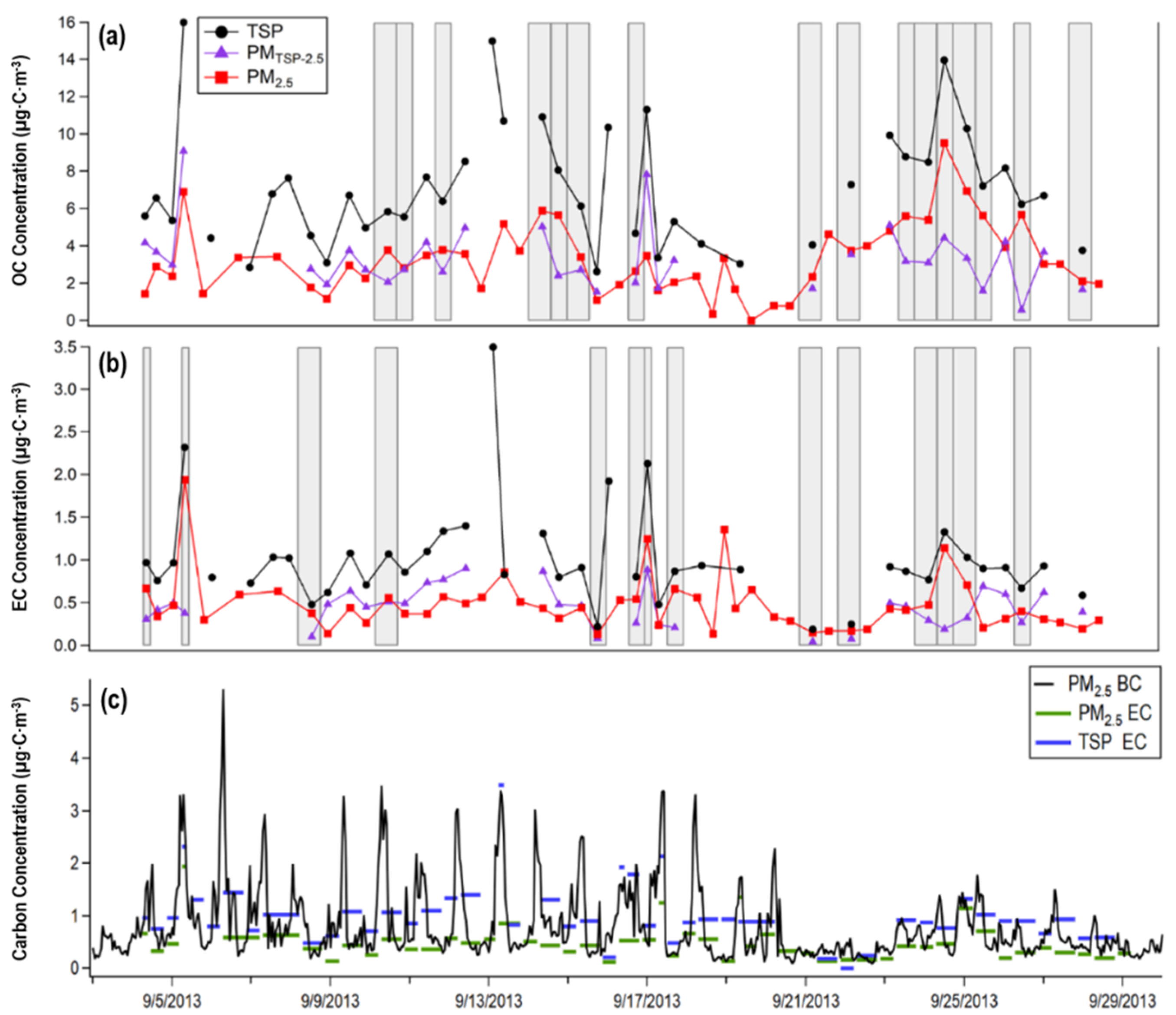
3.1.1. Carbonaceous Aerosols Trends of PM2.5 at MT

Based on the bulk carbon measurement (Table S1), two distinct periods of increased TC concentrations were observed: 8–15 September (week 2; W2) and 21–28 September (week 4; W4), respectively (Figure 2a,b). Both weeks began with several days of increasing TC until reaching a peak concentration followed by a few days of declining TC concentration (Figure 2a,b). The ambient OC concentration for both weeks was statistically larger compared to the rest of the sampling period (t-test; p > 0.05). The temporal trends observed in the MT TC were also observed in PM2.5 mass concentrations measured across the Houston metropolitan area [17,18,20]. The description of these two weeks will be further detailed in a future study [20].
The average PM2.5 OC and EC concentrations during the campaign (morning, afternoon, day, and night) are reported in Table 2 and Table 3. The highest average OC and EC concentrations (±SD) were from the morning (n = 4) with an average of 3.8 ± 2.3 and 1.3 ± 0.5 µg C·m−3, respectively, while afternoon (n = 3) periods had the lowest average concentrations of OC and EC at 2.06 ± 0.72 and 0.34 ± 0.10 µg·C·m−3, respectively. There was no significant difference between morning and daytime OC concentrations (Mann-Whitney test; p > 0.05), while the EC concentration during the morning was significantly higher than the daytime (Mann-Whitney test; p < 0.05). The morning sampling periods (06:00–10:00) were shorter and intended to capture the morning rush hour where emission of carbonaceous aerosol was likely increased due to the influx of MVE emission combined with the lower boundary layer; this will be discussed further in Section 3.1.2 with the hourly BC results. The OC and EC concentrations during the day and nighttime were not significantly different (t-test; p > 0.05).
The PM2.5 OC to EC ratio (OC/EC) was utilized as a qualitative indicator of potential secondary organic aerosol (SOA) contribution [37,38,39]. As EC is a tracer for primary emissions, a higher OC/EC is indicative of enhanced secondary processes. Biomass burning (BB) sources can also contribute to increased OC/EC [38,40]; however, the emission ratio of OC and EC from BB can be highly variable [41,42]. Urban studies have utilized OC/EC for identifying BB contribution generally during the winters as SOA contribution is more prominent during the summer periods [38,43]. For this study, high OC/EC may indicate increased SOA contribution, but BB cannot be ruled out by this method. Average OC/EC during the full campaign period was 8.7 ± 5.8. The average OC/EC (±SD) of PM2.5 for the morning, afternoon, day, and night periods were 2.7 ± 0.6, 6.4 ± 2.3, 9.3 ± 4.7, and 9.8 ± 7.6, respectively. The high nighttime OC/EC is in line with Leong et al. [18] and Bean et al.’s [17] studies, where increased aerosols concentration due to nighttime SOA formation was observed. Unlike nighttime, the morning period (06:00–10:00) was impacted by more primary emissions reflected by increased EC concentration, a lower OC/EC, followed by a near factor of two increase in OC/EC in the afternoon (10:00–20:00) when photochemically driven SOA formation would be more prevalent.
The average OC/EC (±SD) during W2 and W4 was 8.1 ± 3.4 and 14.6 ± 6.4, respectively. The OC/EC was significantly higher during W4 compared to W2 (t-test; p < 0.05). The W4, which included an ozone event, was influenced by high atmospheric processing. Previously published studies identified an increase in processed aerosols and highly oxygenated organic aerosols across the metropolitan area during W4 [17,18]. Southeastern U.S. cities are well known to be impacted by SOA contributions associated with high biogenic emissions in this region [44]. Even so, overall OC/EC from this study was higher than reported for other south and southeastern U.S. cities, including Dallas, TX (summer average: 5.56) [28], Atlanta, GA (3.05), and Centreville, AL (6.31) [45]. They were also much higher than annual and seasonal averages in Los Angeles, CA (annual average: 2.03) [46], and New York City, NY (summer average: 4.0) [47], respectively.

3.1.2. BC and EC Comparison

The average BC concentration (±SD) during the full sampling period was 0.80 ± 0.69 µg·C·m−3. Based on hourly-averaged BC measurements for the entire campaign (Table S3), the highest BC concentrations were between 04:00 and 10:00, peaking at 07:00 (Figure S1). This captures Houston’s morning rush hour [48]. The early start may also be associated with industrial activity near the HSC, including trains and other combustion sources. The morning peak in BC concentration was also present in EC results, where the morning samples had the highest EC concentration (Figure 2b,c). The BC concentration was significantly higher during W2 (average: 0.93 ± 0.21 µg·C·m−3) compared to W4 (0.55 ± 0.22 µg·C·m−3) (t-test; p < 0.05). Defined morning peaks of BC can be observed during W2 but were not present in W4 (Figure 2c). Windrose plots of the BC concentrations in W2 and W4 reveal differences in wind direction between the two weeks (Figure 3). The high BC concentrations, which occurred in the mornings during W2, all come from the East, towards the HSC. This pattern was not observed in the fine EC, where there was no significant difference between W2 (average: 0.43 ± 0.18 µg·C·m−3) and W4 (average: 0.36 ± 0.25 µg·C·m−3) (t-test; p > 0.05). Despite this, the BC was well correlated to the fine and coarse EC with a linear regression r2 value of 0.72 and 0.74, respectively, and a slope of 1.17 with the fine EC. It is not clear why the BC deviates from fine EC with respect to higher concentrations in W2; however, the daily filter change occurred at 06:00–06:30 every morning. This small gap in the filter data record during the peak BC hours may have resulted in a low bias for W2 EC.
The observed daily trend of BC was comparable to measurements made in the spring (April to May) of 2009 during the Study of Houston Atmospheric Radical Precursors (SHARP) field campaign. BC concentrations during SHARP were also high in the early morning with a peak concentration at 07:00 [49]. Average BC and EC concentrations (±SD) during SHARP were 0.31 ± 0.22 and 0.38 ± 0.19 µg·C·m−3, respectively, which is lower than the BC and EC concentrations (±SD) measured for this study in 2013 (average: 0.80 ± 0.69 and 0.48 ± 0.34 µg·C·m−3, respectively). SHARP measurements were made during late spring, while this study was during late summer/fall. EC measurement in both Houston and Dallas have reported higher EC concentrations during the fall and winter periods relative to spring and summer [28], so this may just represent a seasonal difference between SHARP and DISCOVER-AQ.

3.1.3. Carbonaceous Aerosol Trends of TSP

The average TSP OC and EC concentrations (±SD) for the morning, afternoon, day, and night samples are reported in Table 2. The TSP TC concentrations during the day and night were not significantly different (t-test; p > 0.05); however, OC and EC concentrations during the morning were significantly higher than the night (Mann-Whitney test: p < 0.05). This is the same trend observed in the PM2.5 EC and BC. The TSP OC and EC concentrations were not statistically different between the two weeks of interest (W2 and W4) for either daytime (t-test; p > 0.05) or nighttime (Mann-Whitney test; p > 0.05). During the campaign period, the largest TSP OC concentration (±SD) was on the morning of September 5 (16 ± 1.1 µg·C·m−3), while the largest EC concentration was on the morning of September 13 (3.5 ± 0.46 µg·C·m−3, Table 2). The highest non-morning TSP OC concentration (±SD) was during the night of September 24, with a concentration of 13.95 ± 0.83 µg·C·m−3 (Table 2).
The average OC/EC for TSP during the full campaign was 8.2 ± 4.6. The average OC/EC (±SD) for the morning, afternoon, day, and night TSP were 5.5 ± 0.94, 9.5 ± 3.1, 10.1 ± 6.4, and 7.3 ± 2.4, respectively. Unlike the PM2.5, average OC/EC was higher during the day than at night, indicating a larger contribution of non-combustion aerosols during the day. Like the PM2.5, the day–night difference was not significant (t-test; p > 0.05). Sources of coarse OC include resuspension of soil, as well as primary biological aerosol particles (e.g., lignan polymers), which were found to be a relatively important source of coarse aerosol in Houston [50]. The average OC/EC (± SD) for W2 and W4 were 7.5 ± 2.6 and 12 ± 6.6, respectively. Like the PM2.5, the average OC/EC during W4 was significantly higher than the average OC/EC measured during the W2 (t-test; p < 0.05). The carbonaceous aerosol in the W4 was likely impacted by increased secondary processing in the PM2.5, while the TSP also was influenced by a change in atmospheric processing and/or sources in the later week.

3.1.4. Comparison of Carbonaceous Aerosols Between PM2.5 and TSP

Direct comparison between PM2.5 and TSP was possible for 33 samples (three morning, two afternoon, 15 day, and 13 night samples; Figure 2a,b). Although there were few morning and afternoon samples, these were included in the comparison. The OC and EC concentrations for PM2.5 and TSP were strongly correlated (r2 = 0.70 and 0.72, respectively). The PM2.5 to TSP ratio (PM2.5/TSP) for TC, OC, and EC concentrations were each 0.52 with SDs of 0.12, 0.14, and 0.18, respectively. Average PM2.5/TSP (±SD) for OC was slightly higher at night, 0.57 ± 0.16, compared to the day, 0.52 ± 0.09. Within the daytime, the PM2.5/TSP for OC was higher in the afternoon, 0.46 ± 0.03, compared to the mornings, 0.33 ± 0.09. The PM2.5/TSP for OC was also significantly higher during W2 and W4 (0.55 ± 0.13) compared to the other sampling days (0.41 ± 0.10) (t-test; p < 0.05). During these periods of enhanced TC concentrations (W2 and W4), the enhancement in the OC was driven by an increase in fine PM relative to the coarse PM (Figure 2a). In Figure 2a,b, the gray boxes highlight periods when the carbon concentration of the fine PM was greater than the coarse PM. In general, the W2 and W4 periods both had relatively higher OC/EC (PM2.5) and PM2.5/TSP. The results of these qualitative tests support that PM2.5 OC during these periods was enhanced due to secondary processes. SOA formation is via oxidation of gas-phase precursors (e.g., volatile organic compounds (VOC)) and/or condensation of semi-volatile organic compounds. Previous studies, at varying study sites (i.e., urban, marine, and forests), have generally found these photochemically-produced aerosols in the fine and ultrafine aerosol fractions [51,52].
EC is formed from the incomplete combustion of either fossil fuel or BB sources and is typically distributed in the fine to ultrafine particulate fraction [53], but this was not the case for this study. Average PM2.5/TSP (± SD) of EC was largest in the morning (0.70 ± 0.13) relative to afternoon (0.47 ± 0.03), day (0.50 ± 0.17) and night (0.50 ± 0.19) periods. The measured morning periods had higher concentrations of fine than coarse EC (Figure 2b). This was likely due to enhanced contribution of fine EC from MVE or activity associated with the HSC. However, the overall average PM2.5/TSP ratio for EC was 0.52 ± 0.18, which indicates a significant contribution of EC from the coarse fraction. Concentrations of the coarse EC ranged from 0.04–0.90 µg·C·m−3 with an average of 0.44 ± 0.24 µg·C·m−3. Coarse EC has been measured in high concentrations in Karachi, Pakistan (2.9 µg·C·m−3); Lahore, India (~6.3 µg·C·m−3); and Beijing, China (2.0 µg·C·m−3) [54]. Studies have attributed coarse EC to open field or other uncontrolled BB and/or use of less efficient/older technology for industrial combustion processes, including coke ovens, steelmaking, and transportation [31,54,55]. Average coarse EC concentration from this study (0.44± 0.24 µg·C·m−3) was larger than coarse EC (PM10−2.5) measured in other U.S. cities, including Atlanta, GA (urban site; 0.21 ± 0.13 µg·C·m−3), and Centerville, AL (rural site; 0.27 ± 0.16 µg·C·m−3). However, Houston’s coarse EC was significantly less than North Birmingham, AL (urban/industrial site) with an average of 2.70 ± 3.52 µg·C·m−3 [31]. The large concentration of coarse EC in North Birmingham was attributed to local industrial processes, including coke ovens and steel making [31]. The coarse EC in Houston may also be due to the different industrial activities that are close in proximity to the MT site, including a petroleum coke facility along with other industrial operations in the HSC, located approximately 10 km southeast of MT.

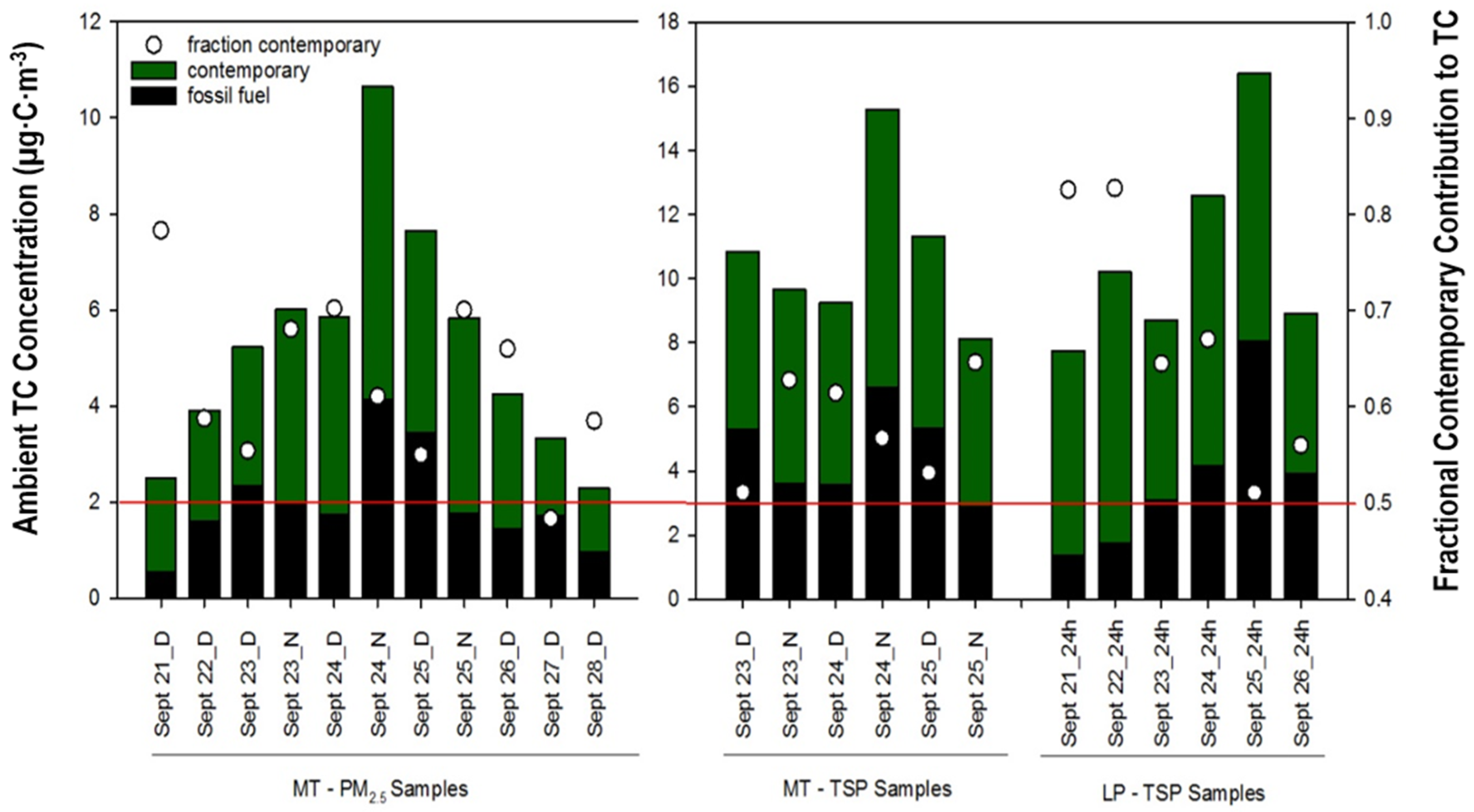
3.2. 14C-based Apportionment of PM2.5 and TSP

Fossil and Contemporary Carbon for TSP versus PM2.5

To better understand the contribution of different sources to the TC, 14C-based source apportionment was performed on PM2.5 and TSP TC for day and night samples during W4 (Table S2). Overall, the contribution of contemporary carbon was larger than fossil carbon for both size fractions at MT and LP. Aside from the daytime PM2.5 on September 27 at MT where contemporary contribution (±SD) was 48 ± 3%, all contemporary contribution of TC (PM2.5 and TSP) was above 50% (Figure 4). For MT PM2.5, the average daytime contemporary carbon contribution and concentration (±SD) during W4 was 61 ± 10% and 2.7 ± 1.1 µg·C·m−3, respectively, while the nighttime (23–25 September) was 65 ± 5% and 4.7 ± 1.2 µg·C·m−3, respectively. In general, daytime carbonaceous aerosols were more impacted by fossil fuel sources, while nighttime aerosols were more impacted by contemporary sources (Figure 4), which could include biogenic SOA or BB. A more detailed examination of the daytime 14C is included in a future manuscript [20]. For MT TSP (day and night samples from 23–25 September), the average contemporary carbon contribution and concentration were 58 ± 5% and 6.2 ± 1.3 µg·C·m−3, respectively. Like the diurnal trends observed in the PM2.5, average contemporary carbon contribution and concentration was greater during the night (61 ± 4% and 6.7 ± 1.8 µg·C·m−3, respectively) than the day (55 ± 5% and 5.75 ± 0.25 µg·C·m−3, respectively). When considering source differences between fine and coarse aerosol, the average ± SD PM2.5/TSP for contemporary carbon was 0.69 ± 0.09, while the fossil carbon was 0.56 ± 0.08. Considered as a percent contribution, the coarse PM had larger contribution from fossil carbon, ranging from 46 to 53%, compared to fine PM, ranging from 30 to 45% for 23–25 September (Figure 4). It is not clear if the source of this coarse fossil TC was associated with industrial activities or is linked to soil/crustal PM.
Within W4, September 24 day to September 25 day has a different trend. The OC and EC concentrations in the fine were greater than coarse PM (Figure 2a,b), and the contemporary carbon contribution decreased. The carbonaceous aerosol during this period was likely driven by secondary processing of fossil carbon emissions specifically impacting the fine particulate fraction.
Source apportionment results from the auxiliary site, LP, reported a larger contribution of contemporary carbon contribution relative to the urban core site at MT. The average ± SD contemporary contribution and concentration of TSP at LP was 67 ± 13% and 7.1 µg·C·m−3, respectively. The average ± SD fossil contribution and concentration for LP was 33 ± 13% and 3.7 ± 2.4 µg·C·m−3, respectively. Though the LP site is closer to the HSC, the contemporary carbon contribution was higher than in MT (day and night) (Figure 4). However, the general trends observed during the W4 at MT for both PM2.5 and TSP were also observed in the LP TSP (Figure 4). The largest contribution and concentration (±SD) of fossil carbon at LP was on September 25 with 49 ± 3% and 8.0 µg·C·m−3 (Figure 4). Both fossil carbon contribution and concentration were higher at LP than at MT (day and night) on 25 September. Previous studies have attributed the high pollution event on 25 September to the bay breeze, where a re-circulation of air mass via continental offshore winds transports it out to the Gulf and then back to Houston city (crossing over the HSC), where the resultant wind speeds across the Houston metropolitan area were low, producing stagnant conditions [22,56]. Point source emissions from Houston’s HSC was another important factor for the high pollution event on 25 September [56,57]. The larger contribution and concentration of fossil carbon observed at LP than at MT on 25 September could be due to LP proximity to this industrial region of Houston.

4. Conclusions

In this study, a detailed characterization of the carbonaceous aerosols for PM2.5 and TSP provided a better understanding of PM sources and trends in Houston. This study (1) identified important diurnal and temporal trends and (2) distinguished major sources and aerosol size fractions contributing to poor air quality days (i.e., increased PM and/or ozone levels) in Houston. Initial bulk carbon analysis identified the highest OC and EC concentrations during mornings for both PM2.5 and TSP. Real-time BC measurements confirmed these morning peaks (i.e., 04:00–10:00). The enhanced OC, EC, and BC concentrations during the morning period were likely due to a combination of increased emissions and favorable meteorological conditions (i.e., low boundary layer). For these mornings, as expected, EC was more enhanced in the fine than the coarse PM, likely due to the incomplete combustion from MVE. The large contribution of coarse EC was also observed during this project, likely from less efficient industrial processes near the Houston MT site.
Overall, the OC/EC was relatively high, especially in the PM2.5 fraction. The OC/EC was high during both W4 and W2. During both weeks, the OC concentration in the fine was larger than the coarse fraction, particularly during W4. The enhanced concentration of carbonaceous aerosol during W4 was driven by OC and EC in the fine fraction. The high OC/EC during this period supports enhanced contribution from secondary processes and/or biomass burning.
Further analysis of W4 was accomplished using 14C analysis to distinguish the contribution and concentration of contemporary and fossil carbon. Overall, Houston aerosol was largely from contemporary sources in both PM2.5 and TSP. However, the coarse TC had more impact from fossil sources than the fine TC, with an average ± SD of 51 ± 3% for coarse and 38 ± 7% for fine aerosol. The LP TSP, relative to MT TSP, had larger variability in contemporary and fossil carbon concentrations. Depending on meteorology and wind patterns, the LP site can be impacted by either strong, clean onshore winds or by industrial emissions. For days with poor air quality, 24 to 25 September, the carbonaceous aerosols were impacted by an increase in fossil carbon contribution at both MT and LP sites but driven by fine PM. This study has identified differences in coarse and fine sources of EC in Houston. Further study is needed to identify the sources of coarse EC and monitor potential seasonal trends.

Supplementary Materials

The following is available online at https://www.mdpi.com/2073-4433/11/5/482/s1, S1: Detailed calculation for BC correction, Figure S1: Hourly averaged ambient BC concentration, including 1 standard deviation error bars; Table S1: Bulk carbon, including OC and EC (and, respectively, uncertainty) ambient concentration for all PM2.5 and TSP samples from MT. Each sample is identified by the sample date (YYMMDD) followed by the sampling period which includes morning (M), afternoon (A), day (D), night (N), and 24-h samples; Table S2: Contemporary and fossil carbon (and respective uncertainty) ambient concentration of TC from 14C analysis and its uncertainty for all PM2.5 and TSP samples from MT. Samples from Moody Tower (MT) and La Porte (LP) are included. Each sample is identified by the sample date (YYMMDD) followed by the sampling period which includes day (D), night (N) and 24-h samples; Table S3: Hourly-averaged ambient BC concentration during sampling period. Dates are formatted as YYMMDD.

Author Contributions

Conceptualization, S.Y. and R.J.S.; formal analysis, S.Y.; data curation, S.Y.; investigation, S.Y.; writing—original draft, S.Y.; writing—review and editing, S.U. and R.J.S.; supervision, R.J.S.; project administration, R.J.S.; funding acquisition, S.U. and R.J.S. All authors have read and agreed to the published version of the manuscript.

Funding

The preparation of this manuscript was financed through a grant from the Texas Commission on Environmental Quality (TCEQ, grant number 12-032 and 14-029), administered by the University of Texas at Austin, Center for Energy and Environmental Resources (CEER) through the Air Quality Research Program (AQRP). The contents findings, opinions, and conclusions are the work of the authors and do not necessarily represent findings, opinions, or conclusions of the TCEQ. Additional funding was provided by the C. Gus Glasscock, Jr. Endowed Fund for Excellence in Environmental Sciences.

Acknowledgments

The authors would like to acknowledge the U.S. Environmental Protection Agency, especially Rachelle Duvall and Russell Long, for providing a Tisch PM2.5 sampler used at MT and for sample collection at LP. The authors would also like to thank James Schauer of the University of Wisconsin–Madison for providing two Tisch high volume TSP samplers used at MT and LP. In addition, the authors would like to thank Raj B. Nadkarni and Jim Thomas at Texas Commission on Environmental Quality for site access and support.

Conflicts of Interest

The authors declare no financial conflict of interest.

References

  1. Chung, C.E.; Ramanathan, V.; Decremer, D. Observationally constrained estimates of carbonaceous aerosol radiative forcing. Proc. Natl. Acad. Sci. USA 2012, 109, 11624–11629. [Google Scholar] [CrossRef] [Green Version]
  2. Spracklen, D.; Carslaw, K.; Pöschl, U.; Rap, A.; Forster, P. Global cloud condensation nuclei influenced by carbonaceous combustion aerosol. Atmos. Chem. Phys. 2011, 11, 9067–9087. [Google Scholar] [CrossRef] [Green Version]
  3. Novakov, T.; Penner, J. Large contribution of organic aerosols to cloud-condensation-nuclei concentrations. Nature 1993, 365, 823–826. [Google Scholar] [CrossRef]
  4. Kanakidou, M.; Seinfeld, J.; Pandis, S.; Barnes, I.; Dentener, F.; Facchini, M.; Dingenen, R.V.; Ervens, B.; Nenes, A.; Nielsen, C. Organic aerosol and global climate modelling: A review. Atmos. Chem. Phys. 2005, 5, 1053–1123. [Google Scholar] [CrossRef] [Green Version]
  5. Tsigaridis, K.; Daskalakis, N.; Kanakidou, M.; Adams, P.; Artaxo, P.; Bahadur, R.; Balkanski, Y.; Bauer, S.; Bellouin, N.; Benedetti, A. The AeroCom evaluation and intercomparison of organic aerosol in global models. Atmos. Chem. Phys. 2014, 14, 10845–10895. [Google Scholar] [CrossRef] [Green Version]
  6. Dockery, D.W.; Pope, C.A. Acute respiratory effects of particulate air pollution. Ann. Rev. Public Health 1994, 15, 107–132. [Google Scholar] [CrossRef]
  7. Brook, R.D.; Rajagopalan, S.; Pope, C.A.; Brook, J.R.; Bhatnagar, A.; Diez-Roux, A.V.; Holguin, F.; Hong, Y.; Luepker, R.V.; Mittleman, M.A. Particulate matter air pollution and cardiovascular disease: An update to the scientific statement from the American Heart Association. Circulation 2010, 121, 2331–2378. [Google Scholar] [CrossRef] [Green Version]
  8. Laden, F.; Neas, L.M.; Dockery, D.W.; Schwartz, J. Association of fine particulate matter from different sources with daily mortality in six US cities. Environ. Health Perspect. 2000, 108, 941. [Google Scholar] [CrossRef]
  9. Delfino, R.J.; Murphy-Moulton, A.M.; Becklake, M.R. Emergency room visits for respiratory illnesses among the elderly in Montreal: Association with low level ozone exposure. Environ. Res. 1998, 76, 67–77. [Google Scholar] [CrossRef]
  10. Chen, R.; Zhao, Z.; Kan, H. Heavy smog and hospital visits in Beijing, China. Am. J. Respir. Crit. Care Med. 2013, 188, 1170–1171. [Google Scholar] [CrossRef]
  11. United States Census Burea: QuickFacts Houston City, Texas. Available online: https://www.census.gov/quickfacts/fact/table/houstoncitytexas/PST045219 (accessed on 28 January 2020).
  12. Sullivan, D.W.; Price, J.H.; Lambeth, B.; Sheedy, K.A.; Savanich, K.; Tropp, R.J. Field study and source attribution for PM2.5 and PM10 with resulting reduction in concentrations in the neighborhood north of the Houston Ship Channel based on voluntary efforts. J. Air Waste Manag. Assoc. 2013, 63, 1070–1082. [Google Scholar] [CrossRef] [PubMed] [Green Version]
  13. Wallace, H.W.; Sanchez, N.P.; Flynn, J.H.; Erickson, M.H.; Lefer, B.L.; Griffin, R.J. Source apportionment of particulate matter and trace gases near a major refinery near the Houston Ship Channel. Atmos. Environ. 2018, 173, 16–29. [Google Scholar] [CrossRef]
  14. Zhang, X.; Craft, E.; Zhang, K. Characterizing spatial variability of air pollution from vehicle traffic around the Houston Ship Channel area. Atmos. Environ. 2017, 161, 167–175. [Google Scholar] [CrossRef]
  15. Schulze, B.C.; Wallace, H.W.; Bui, A.T.; Flynn, J.H.; Erickson, M.H.; Alvarez, S.; Dai, Q.; Usenko, S.; Sheesley, R.J.; Griffin, R.J. The impacts of regional shipping emissions on the chemical characteristics of coastal submicron aerosols near Houston, TX. Atmos. Chem. Phys. 2018, 18, 14217–14241. [Google Scholar] [CrossRef] [Green Version]
  16. Park, C.; Schade, G.W.; Boedeker, I. Characteristics of the flux of isoprene and its oxidation products in an urban area. J. Geophys. Res. Atmos. 2011, 116, D21303. [Google Scholar] [CrossRef] [Green Version]
  17. Bean, J.K.; Faxon, C.B.; Leong, Y.J.; Wallace, H.W.; Cevik, B.K.; Ortiz, S.; Canagaratna, M.R.; Usenko, S.; Sheesley, R.J.; Griffin, R.J. Composition and Sources of Particulate Matter Measured near Houston, TX: Anthropogenic-Biogenic Interactions. Atmosphere 2016, 7, 73. [Google Scholar] [CrossRef] [Green Version]
  18. Leong, Y.; Sanchez, N.; Wallace, H.; Cevik, B.K.; Hernandez, C.; Han, Y.; Flynn, J.; Massoli, P.; Floerchinger, C.; Fortner, E. Overview of surface measurements and spatial characterization of submicrometer particulate matter during the DISCOVER-AQ 2013 campaign in Houston, TX. J. Air Waste Manag. Assoc. 2017, 67, 854–872. [Google Scholar] [CrossRef]
  19. DISCOVER-AQ. Available online: https://discover-aq.larc.nasa.gov/ (accessed on 1 August 2015).
  20. Yoon, S.; Ortiz, S.; Clark, A.E.; Barrett, T.E.; Usenko, S.; Duvall, R.M.; Ruiz, L.H.; Bean, J.K.; Faxon, C.B.; Flynn, J.; et al. Apportioned primary and secondary organic aerosol during pollution events of DISCOVER-AQ Houston. Atmos. Environ. under review.
  21. Mazzuca, G.M.; Ren, X.; Loughner, C.P.; Estes, M.; Crawford, J.H.; Pickering, K.E.; Weinheimer, A.J.; Dickerson, R.R. Ozone production and its sensitivity to NOx and VOCs: Results from the DISCOVER-AQ field experiment, Houston 2013. Atmos. Chem. Phys. 2016, 16, 14463–14474. [Google Scholar] [CrossRef] [Green Version]
  22. Baier, B.C.; Brune, W.H.; Lefer, B.L.; Miller, D.O.; Martins, D.K. Direct ozone production rate measurements and their use in assessing ozone source and receptor regions for Houston in 2013. Atmos. Environ. 2015, 114, 83–91. [Google Scholar] [CrossRef]
  23. Hansen, A.; Rosen, H.; Novakov, T. Aethalometer—An Instrument for the Real-Time Measurement of Optical Absorption by Aerosol Particles; Lawrence Berkeley Lab.: Berkeley, CA, USA, 1983. [Google Scholar]
  24. Chow, J.C.; Watson, J.G.; Crow, D.; Lowenthal, D.H.; Merrifield, T. Comparison of IMPROVE and NIOSH carbon measurements. Aerosol Sci. Technol. 2001, 34, 23–34. [Google Scholar] [CrossRef]
  25. Clark, A.E.; Yoon, S.; Sheesley, R.J.; Usenko, S. Pressurized liquid extraction technique for the analysis of pesticides, PCBs, PBDEs, OPEs, PAHs, alkanes, hopanes, and steranes in atmospheric particulate matter. Chemosphere 2015, 137, 33–44. [Google Scholar] [CrossRef]
  26. Birch, M.; Cary, R. Elemental carbon-based method for monitoring occupational exposures to particulate diesel exhaust. Aerosol Sci. Technol. 1996, 25, 221–241. [Google Scholar] [CrossRef]
  27. Schauer, J.J. Evaluation of elemental carbon as a marker for diesel particulate matter. J. Expo. Sci. Environ. Epidemiol. 2003, 13, 443–453. [Google Scholar] [CrossRef] [PubMed] [Green Version]
  28. Barrett, T.E.; Sheesley, R.J. Urban impacts on regional carbonaceous aerosols: Case study in central Texas. J. Air Waste Manag. Assoc. 2014, 64, 917–926. [Google Scholar] [CrossRef] [PubMed] [Green Version]
  29. Cachier, H.; Bremond, M.-P.; Buat-Menard, P. Determination of atmospheric soot carbon with a simple thermal method. Tellus B 1989, 41, 379–390. [Google Scholar] [CrossRef] [Green Version]
  30. Tian, S.; Pan, Y.; Liu, Z.; Wen, T.; Wang, Y. Reshaping the size distribution of aerosol elemental carbon by removal of coarse mode carbonates. Atmos. Environ. 2019, 214, 116852. [Google Scholar] [CrossRef]
  31. Edgerton, E.S.; Casuccio, G.S.; Saylor, R.D.; Lersch, T.L.; Hartsell, B.E.; Jansen, J.J.; Hansen, D.A. Measurements of OC and EC in coarse particulate matter in the southeastern United States. J. Air Waste Manag. Assoc. 2009, 59, 78–90. [Google Scholar] [CrossRef]
  32. Snyder, D.C.; Schauer, J.J. An inter-comparison of two black carbon aerosol instruments and a semi-continuous elemental carbon instrument in the urban environment. Aerosol Sci. Technol. 2007, 41, 463–474. [Google Scholar] [CrossRef] [Green Version]
  33. Schmid, O.; Artaxo, P.; Arnott, W.; Chand, D.; Gatti, L.V.; Frank, G.; Hoffer, A.; Schnaiter, M.; Andreae, M. Spectral light absorption by ambient aerosols influenced by biomass burning in the Amazon Basin. I: Comparison and field calibration of absorption measurement techniques. Atmos. Chem. Phys. 2006, 6, 3443–3462. [Google Scholar] [CrossRef] [Green Version]
  34. Stuiver, M.; Polach, H.A. Discussion; reporting of C-14 data. Radiocarbon 1977, 19, 355–363. [Google Scholar] [CrossRef] [Green Version]
  35. Zotter, P.; El-Haddad, I.; Zhang, Y.; Hayes, P.L.; Zhang, X.; Lin, Y.H.; Wacker, L.; Schnelle-Kreis, J.; Abbaszade, G.; Zimmermann, R. Diurnal cycle of fossil and nonfossil carbon using radiocarbon analyses during CalNex. J. Geophys. Res. Atmos. 2014, 119, 6818–6835. [Google Scholar] [CrossRef] [Green Version]
  36. Gustafsson, Ö.; Kruså, M.; Zencak, Z.; Sheesley, R.J.; Granat, L.; Engström, E.; Praveen, P.; Rao, P.; Leck, C.; Rodhe, H. Brown clouds over South Asia: Biomass or fossil fuel combustion? Science 2009, 323, 495–498. [Google Scholar] [CrossRef] [PubMed]
  37. Chow, J.C.; Watson, J.G.; Fujita, E.M.; Lu, Z.; Lawson, D.R.; Ashbaugh, L.L. Temporal and spatial variations of PM2.5 and PM10 aerosol in the Southern California air quality study. Atmos. Environ. 1994, 28, 2061–2080. [Google Scholar] [CrossRef]
  38. Benetello, F.; Squizzato, S.; Hofer, A.; Masiol, M.; Khan, M.B.; Piazzalunga, A.; Fermo, P.; Formenton, G.M.; Rampazzo, G.; Pavoni, B. Estimation of local and external contributions of biomass burning to PM 2.5 in an industrial zone included in a large urban settlement. Environ. Sci. Pollut. Res. 2017, 24, 2100–2115. [Google Scholar] [CrossRef]
  39. Turpin, B.J.; Huntzicker, J.J. Identification of secondary organic aerosol episodes and quantitation of primary and secondary organic aerosol concentrations during SCAQS. Atmos. Environ. 1995, 29, 3527–3544. [Google Scholar] [CrossRef]
  40. Ram, K.; Sarin, M. Day–night variability of EC, OC, WSOC and inorganic ions in urban environment of Indo-Gangetic Plain: Implications to secondary aerosol formation. Atmos. Environ. 2011, 45, 460–468. [Google Scholar] [CrossRef]
  41. Zhang, Y.; Zotter, P.; Perron, N.; Prévôt, A.; Wacker, L.; Szidat, S. Fossil and non-fossil sources of different carbonaceous fractions in fine and coarse particles by radiocarbon measurement. Radiocarbon 2013, 55, 1510–1520. [Google Scholar] [CrossRef] [Green Version]
  42. Hong, L.; Liu, G.; Zhou, L.; Li, J.; Xu, H.; Wu, D. Emission of organic carbon, elemental carbon and water-soluble ions from crop straw burning under flaming and smoldering conditions. Particuology 2017, 31, 181–190. [Google Scholar] [CrossRef]
  43. Viana, M.; Maenhaut, W.; Brink, H.T.; Chi, X.; Weijers, E.; Querol, X.; Alastuey, A.; Mikuška, P.; Večeřa, Z. Comparative analysis of organic and elemental carbon concentrations in carbonaceous aerosols in three European cities. Atmos. Environ. 2007, 41, 5972–5983. [Google Scholar] [CrossRef] [Green Version]
  44. Zeng, T.; Wang, Y. Nationwide summer peaks of OC/EC ratios in the contiguous United States. Atmos. Environ. 2011, 45, 578–586. [Google Scholar] [CrossRef]
  45. Blanchard, C.L.; Hidy, G.M.; Tanenbaum, S.; Edgerton, E.; Hartsell, B.; Jansen, J. Carbon in southeastern US aerosol particles: Empirical estimates of secondary organic aerosol formation. Atmos. Environ. 2008, 42, 6710–6720. [Google Scholar] [CrossRef]
  46. Kim, B.M.; Teffera, S.; Zeldin, M.D. Characterization of PM25 and PM10 in the South Coast air basin of Southern California: Part 1—Spatial variations. J. Air Waste Manag. Assoc. 2000, 50, 2034–2044. [Google Scholar] [CrossRef] [PubMed]
  47. Rattigan, O.V.; Felton, H.D.; Bae, M.-S.; Schwab, J.J.; Demerjian, K.L. Multi-year hourly PM2.5 carbon measurements in New York: Diurnal, day of week and seasonal patterns. Atmos. Environ. 2010, 44, 2043–2053. [Google Scholar] [CrossRef]
  48. Czader, B.H.; Choi, Y.; Li, X.; Alvarez, S.; Lefer, B. Impact of updated traffic emissions on HONO mixing ratios simulated for urban site in Houston, Texas. Atmos. Chem. Phys. 2015, 15, 1253–1263. [Google Scholar] [CrossRef] [Green Version]
  49. Levy, M.E.; Zhang, R.; Khalizov, A.F.; Zheng, J.; Collins, D.R.; Glen, C.R.; Wang, Y.; Yu, X.Y.; Luke, W.; Jayne, J.T. Measurements of submicron aerosols in Houston, Texas during the 2009 SHARP field campaign. J. Geophys. Res. Atmos. 2013, 118, 10518–10534. [Google Scholar] [CrossRef]
  50. Shakya, K.M.; Louchouarn, P.; Griffin, R.J. Lignin-derived phenols in Houston aerosols: Implications for natural background sources. Environ. Sci. Technol. 2011, 45, 8268–8275. [Google Scholar] [CrossRef]
  51. Kavouras, I.G.; Stephanou, E.G. Particle size distribution of organic primary and secondary aerosol constituents in urban, background marine, and forest atmosphere. J. Geophys. Res. Atmos. 2002, 107, AAC 7-1–AAC 7-12. [Google Scholar] [CrossRef] [Green Version]
  52. Shiraiwa, M.; Yee, L.D.; Schilling, K.A.; Loza, C.L.; Craven, J.S.; Zuend, A.; Ziemann, P.J.; Seinfeld, J.H. Size distribution dynamics reveal particle-phase chemistry in organic aerosol formation. Proc. Natl. Acad. Sci. USA 2013, 110, 11746–11750. [Google Scholar] [CrossRef] [Green Version]
  53. Offenberg, J.H.; Baker, J.E. Aerosol size distributions of elemental and organic carbon in urban and over-water atmospheres. Atmos. Environ. 2000, 34, 1509–1517. [Google Scholar] [CrossRef]
  54. Shahid, I.; Kistler, M.; Mukhtar, A.; Ghauri, B.M.; Ramirez-Santa Cruz, C.; Bauer, H.; Puxbaum, H. Chemical characterization and mass closure of PM10 and PM2.5 at an urban site in Karachi–Pakistan. Atmos. Environ. 2016, 128, 114–123. [Google Scholar] [CrossRef]
  55. Lee, T.; Yu, X.-Y.; Ayres, B.; Kreidenweis, S.M.; Malm, W.C.; Collett, J.L., Jr. Observations of fine and coarse particle nitrate at several rural locations in the United States. Atmos. Environ. 2008, 42, 2720–2732. [Google Scholar] [CrossRef]
  56. Caicedo, V.; Rappenglueck, B.; Cuchiara, G.; Flynn, J.; Ferrare, R.; Scarino, A.; Berkoff, T.; Senff, C.; Langford, A.; Lefer, B. Bay Breeze and Sea Breeze Circulation Impacts on the Planetary Boundary Layer and Air Quality From an Observed and Modeled DISCOVER-AQ Texas Case Study. J. Geophys. Res. Atmos. 2019, 124, 7359–7378. [Google Scholar] [CrossRef]
  57. Dunker, A.M.; Koo, B.; Yarwood, G. Source apportionment of organic aerosol and ozone and the effects of emission reductions. Atmos. Environ. 2019, 198, 89–101. [Google Scholar] [CrossRef]
Figure 1. Map of the Moody Tower (MT) and La Porte (LP) sampling sites. Map includes outline of the city of Houston.
Atmosphere 11 00482 g001
Figure 2. Carbonaceous aerosol concentrations at MT during the full sampling campaign. Figure includes filter-based (a) OC and (b) EC concentration of TSP, PM2.5, and the calculated coarse PM. For (a), (b) The lines between each marker indicate continuous filter collection, while the gray boxes highlight samples where carbon concentrations were higher in the fine than the coarse PM. (c) Hourly-averaged black carbon (BC) and filter-based PM2.5 and TSP EC concentration. The filter-based samples include morning, afternoon, day, and night samples.
Atmosphere 11 00482 g002
Figure 3. Windrose plots for BC concentration during (a) week 2 and (b) week 4 at MT. The radius axis indicates the percent contribution of wind direction sector relative to total week. The BC concentration is indicated by color, with different scales for Week 2 and Week 4.
Atmosphere 11 00482 g003
Figure 4. Radiocarbon-based apportionment of ambient total carbon concentration (left-axis) and fractional contemporary contribution (right-axis) of PM2.5 day (D) and calculated night (N) samples and TSP D and N samples at MT. Apportioned TSP 24-h filter samples from LP are also included. Red line is a marker for the 0.5 contemporary carbon contribution of total carbon (TC).
Atmosphere 11 00482 g004
Table 1. Description of filter samples for reported filter-based analysis. MT = Moody Tower; LP = La Porte; PM = particulate matter; TSP = total suspended particulate; MV = medium volume; HV = high volume; OC = organic carbon; EC = elemental carbon.
SiteSize FractionSampler TypeSamples Sample DurationAnalysis
MTPM2.5Tisch4–28 Septembermorning, afternoon, dayOC EC
21–28 Septemberday14C
MV URG6–28 September24-hOC EC
23–25 September24-h14C
LPTSPHV Tisch4–28 Septembermorning, afternoon, day, night, 24-h OC EC
23–25 Septemberday and night14C
HV Tisch21–26 September24-h OC EC, 14C
Table 2. The average and maximum concentration of OC for the different (morning, afternoon, day, and night) PM2.5 and TSP samples at Moody Tower. The number of samples for each sample type and the sample day for maximum OC concentrations are also included.
PM TypeSample TypeSample No.Average OC (±SD) (µg·C·m−3)Max. OC SampleMax. OC Conc (µg·C·m−3)
PM2.5morning43.79 ± 2.275 September6.90 ± 0.71
afternoon32.06 ± 0.724 September2.89 ± 0.27
day193.55 ± 1.5625 September6.94 ± 0.44
night 1223.21 ± 2.2524 September9.51 ± 0.89
TSPmorning511.64 ± 4.135 September15.98 ± 1.14
afternoon36.87 ± 3.6713 September10.69 ± 0.78
day167.24 ± 2.1214 September10.92 ± 0.60
night166.07 ± 2.7824 September13.95 ± 0.83
1 includes calculated night carbon concentration from PMTSP (24-h) and PM2.5 (morning and afternoon or day) samples.
Table 3. The average and maximum concentration of EC for the different (morning, afternoon, day, and night) PM2.5 and TSP samples at Moody Tower. The number of samples for each sample type and the sample day for maximum EC concentrations are also included.
PM TypeSample TypeSample No.Average EC (±SD) (µg·C·m−3)Max. EC SampleMax. EC Conc (µg·C·m−3)
PM2.5morning41.30 ± 0.52September 51.94 ± 0.40
afternoon30.34 ± 0.10September 190.43 ± 0.14
day190.43 ± 0.18September 130.86 ± 0.12
night 1220.40 ± 0.24September 241.14 ± 0.21
TSPmorning52.17 ± 0.90September 133.49 ± 0.46
afternoon30.69 ± 0.18September 130.83 ± 0.28
day160.87 ± 0.34September 121.40 ± 0.16
night160.84 ± 0.26September 111.34 ± 0.20
1 includes calculated night carbon concentration from PMTSP (24-h) and PM2.5 (morning and afternoon or day) samples.

