Article

Evaluating the Spectral and Physiological Responses of Grapevines (Vitis vinifera L.) to Heat and Water Stresses under Different Vineyard Cooling and Irrigation Strategies

1
Department of Land, Environmental, Agriculture and Forestry, University of Padova, 35020 Legnaro, PD, Italy
2
Waite Research Institute, School of Agriculture, Food and Wine, The University of Adelaide, Glen Osmond, Adelaide, SA 5064, Australia
3
School of Biosciences, University of Nottingham Malaysia, Semenyih 43500, Selangor Darul Ehsan, Malaysia
4
Department of Agronomy, Food, Natural Resources, Animals and the Environment, University of Padova, 35020 Legnaro, PD, Italy
*
Author to whom correspondence should be addressed.
Agronomy 2021, 11(10), 1940; https://doi.org/10.3390/agronomy11101940
Submission received: 3 September 2021 / Revised: 20 September 2021 / Accepted: 23 September 2021 / Published: 27 September 2021

Abstract

:
Heat stress (HS) and water stress (WS) pose severe threats to viticulture, and effective management solutions to counter their effects on grapevine performance must be examined. In this study, we evaluated the physiological and spectral responses of Vitis vinifera L. cv. Sauvignon blanc to individual (HS) and combined (HS + WS) stress under four different cooling and irrigation strategies. The treatments were: standard drip irrigation (SI), extra drip irrigation (SI+), extra sprinklers irrigation (SPRI), and sustained deficit irrigation (SDI; 50% of SI). Compared to the other treatments, in the early stages after the occurrence of HS, the vine water status of SPRI and SI+ improved, with high stomatal conductance (gs) (SPRI) and stem water potential ( Ψ stem; SPRI and SI+). All the physiological indicators measured were significantly lower after the end of HS in the SDI treatment. We also identified the spectral response of grapevine to HS and combined HS and WS (resulting from SDI). Consistent with the physiological analysis, the proximal spectral responses of leaves identified SPRI and SI+ as putative cooling strategies to minimize vine HS. The vines undergoing combined stress (SDI) showed greenness amelioration 10 days after stress, as revealed by the greenness vegetation indices (VIs), i.e., Green Index (GI), Normalized Difference Greenness Vegetation Index (NDGI), and Visible Atmospherically Resistant Index (VARI). However, their physiological recovery was not achieved within this time, as shown by the Simple Ratio Index (SRI), Transformed Chlorophyll Absorption Ratio Index (TCARI), and TCARI/Optimized Soil-Adjusted Vegetation Index (TCARI/OSAVI). A three-step band selection process allowed the identification of the spectral traits’ responsive to HS and combined stress, i.e., 1336–1340 nm, 1967–1971 nm, and 600–604 nm.

Graphical Abstract

1. Introduction

One of the consequences of climate change is the increased frequency, duration and intensity of heatwaves [1,2]. Heatwaves, defined as the persistence of three or more days at or above 35 °C [3], are affecting viticultural areas globally, especially in Europe [4,5,6] and Australia [7,8]. Current projections estimate that heatwaves will further increase by 2100 [9,10].
The effects of heat stress (HS) on grapevine physiology have been studied. The inhibition of net photosynthesis (Pn) caused by HS can lead to lower yield in several grapevine varieties [6,7]. Grape berry maturation may be delayed [11], with a consequent reduction in the size and fresh weight [7] and increased shriveling of berries [12,13]. A decoupling between anthocyanins and sugar was observed in Shiraz and Cabernet Franc under high-temperature conditions [14], and rotundone concentrations were reduced in Shiraz wines [15].
Given the environmental conditions of high temperature and low relative humidity (RH) that occur during a heatwave, if soil water is limited, HS is associated with water stress (WS), due to the increased evaporative demand [16]. WS affects the morphological traits (e.g., reduction in leaf size and vegetative growth) and physiological traits (e.g., reduction in Pn, stomatal conductance—gs, and leaf transpiration rate—E) of vegetation [17]. Although moderate WS increases the quality of red varieties, e.g., promoting the accumulation of quality-related metabolites, it substantially reduces berry size and yield [18]. Moreover, WS may cause oxidative damage via the production of reactive oxygen species, which damage the cells and their components [19]. To date, less attention has been paid to the combined effects of HS and WS on grapevines. Some studies have underlined that the consequences of combined stresses may be substantially different from those of individuals stresses. For example, combined HS and WS leads to increased leaf temperature due to stomatal closure, whereas during individual HS, heat is dissipated through stomata [20].
Application of evaporative cooling via sprinklers or drip irrigation may lead to an improvement in the soil water balance [21], improving vine water status and reducing HS. For example, small amounts of water distributed for three minutes every 15 min by overhead sprinklers lowered the ambient temperature around the canopy by 7 to 10 °C and raised the humidity from 10 to 20% in Tokay [22]. In-canopy misters reduced the canopy temperature of Sauvignon blanc and Cabernet Sauvignon grapevines by 5 °C [23].
Previous studies investigated the physiological response of grapevines to HS and WS under different water management schemes. Edwards et al. [24] studied the effects of a heatwave generated in a glasshouse on Cabernet Sauvignon physiology under regular and deficit irrigation. Their findings showed that gs of deficit-irrigated vines was reduced by more than 85%, Pn by 30%, and internal CO2 concentration (Ci) by 9%. Sousa et al. [25] analyzed the changes in several physiological parameters in Aragonês under different water regimes. Their results revealed that gs, and E were significantly correlated with soil water content, and leaf water potential ( Ψ L) exhibited poorer performance compared to the previous indicators. On the contrary, Ψ L was considered a good indicator of vine water status in Pinot noir under three water management strategies [26].
An accurate estimation of the physiological behavior of grapevine under stress conditions entails the use of complex and, in some cases, destructive equipment. Non-destructive techniques to quantify the effects of extreme weather events on crops are emerging using reflectance or spectral techniques [27]. For example, the green (550 and 570 nm), red (670 nm), red edge (>700 nm), and near-infrared (NIR, 800 nm) spectral bands can provide a reliable prediction of Carménère water status [28]. The NIR spectral band can provide a reliable assessment of the water status of leaves and canopy [29]. Environmental RH during HS correlated positively with the red edge region and growing degree days correlated negatively with the short wave near-infrared (SWIR, 1610 nm) region [3]. There are a wide range of spectral vegetation indices (VIs) used to describe WS, and some preliminary studies have been conducted on HS. Although a considerable number of studies have been carried out to assess the physiological and spectral responses of grapevine WS, specific knowledge of these responses under combined stresses and HS with different evaporative cooling systems is lacking. To the best of our knowledge, the validation of the spectral response with an accurate physiological analysis has not been performed.
In this study, three methods of evaporative cooling were investigated on Vitis vinifera L. cv. Sauvignon blanc under HS conditions in the Riverland region of South Australia. Moreover, a fourth treatment, namely sustained deficit irrigation, was evaluated. The specific objectives of this study were to: (i) evaluate the physiological responses to HS of Vitis vinifera L. cv. Sauvignon blanc under different cooling treatments, and the interactions with WS; and (ii) identify the most consistent, robust, and reliable spectral predictors (hyperspectral bands and VIs) of the physiological responses to HS, and combined WS and HS, and the effects of various evaporative cooling systems. These objectives aimed at verifying our hypotheses that (i) evaporative cooling systems can minimize the physiological effects of HS; and (ii) spectral sensors can be used to assess the physiological responses of grapevines under HS and combined stresses. Testing hypothesis (i) may allow for decision making around management strategies, specifically evaporative cooling systems and irrigation, to reduce the adverse effects of HS on vine performance and grape/wine quality. Moreover, verifying hypothesis (ii) contributes to unravelling the poorly known effects of concurrent HS and WS on grapevines, and identifying non-destructive tools to assess HS in vineyards. Our study proposed a methodological approach that uses an integrated instrumental approach to analyze HS and combined HS and WS. Moreover, the study provided field results during a particularly critical season.

2. Materials and Methods

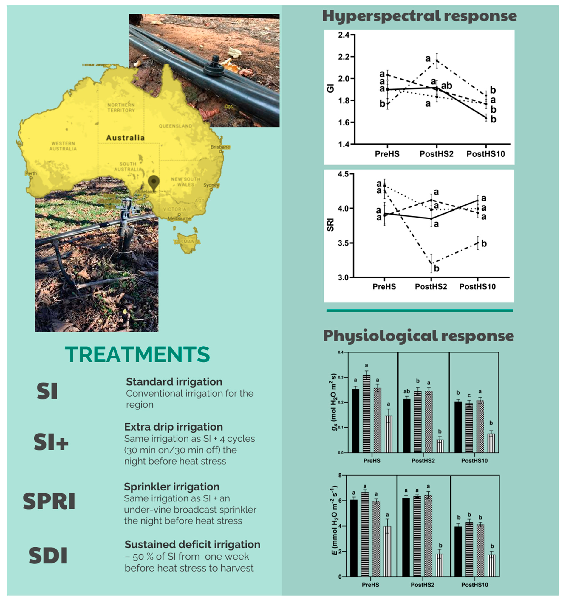
2.1. Study Area and Experimental Design

The study was conducted in January 2020 at Yalumba Oxford Landing Estate (OLE), a commercial vineyard (Figure 1) in the Riverland, South Australia (34°06′06.29″ S and 139°50′39.21″ E). The vineyard block (0.9 ha) was planted in 1995 with Vitis vinifera L. cv. Sauvignon blanc, clone H10-F4V6, rootstock Ramsey, and was 100% mechanizable [30]. Rows were orientated N–S at a spacing of 1.8 m between vines and 3.0 m between rows (approx. 1852 vines ha−1). The vines were trained to the Quadrilateral cordon training system, and their height was approximatively 2.3 m. The topsoil layer (5–25 cm) was loamy sand, and the subsoil sandy loam to loamy sand. There are not known water tables in the top 3.5 m of the soil profile.
The experimental design consisted of the implementation of four irrigation strategies with 24 replicate vines per treatment in a 3 × 3 Latin Square experimental design with at least two rows as buffer within treatments. Therefore, the total number of vines considered in this study was 96. The four treatments were:
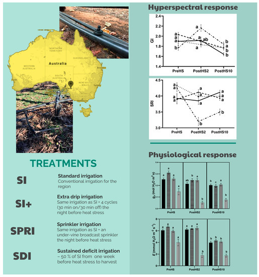
  • Standard drip irrigation (SI)—conventional irrigation for the region, growers applied 4 h of additional irrigation during the day preceding HS. Irrigation was applied using a single dripline with pressure-compensating emitters spaced 0.3 m apart, each with a flow rate of 1 L h−1. This spacing and flow rate delivered approximately 6 L vine−1 h−1, 1.11 mm h−1.
  • Extra drip irrigation (SI+)—same irrigation as SI and, in addition, four cycles of 30 min on/30 min off were triggered at night before HS. The treatment consisted of a separated irrigation line with two drippers per vine (flow rate: 13.5 L h−1). The target flow rate was 54 L vine−1 night−1. The system was controlled with a Galcon G.S.I. DC power wireless solenoid controller.
  • Sprinkler irrigation (SPRI)—the treatment consisted of the same irrigation as SI, and, in addition, an under-vine broadcast sprinkler covering both the under-vine and inter-row regions. Timing and volume of water were the same as SI+. The system was controlled with a Galcon G.S.I. DC power wireless solenoid controller.
  • Sustained deficit irrigation (SDI)—50% of SI from approximatively one week before HS (approximatively two weeks post véraison) to harvest.
The additional amount of water in SI+ and SPRI was provided during the night to minimize evaporative losses from the soil.
In assessing soil/vine responses to deficit irrigation, the water balance method for estimating irrigation requirements is not considered an appropriate technique, and, instead, indicators based on plant water status have been recommended [31]. Therefore, the level of deficit irrigation implemented in SDI was assessed based on significantly different Ψstem.

2.2. Meteorological Data

The meteorological data (average and maximum daily air and soil temperature; average and minimum daily relative humidity; maximum daily vapor pressure deficit; average and maximum daily solar radiation) were obtained from an onsite automatic weather station (AWS) located approximatively 1 km from the trial block. The station is part of the Natural Resources Management (NRM) weather station network, and data are accessible online (https://www.awsnetwork.com.au/station/2770, accessed on 1 March 2021).
The field campaigns took place between the 10 and 25 January 2020. The sampling dates were based on weather forecasts. The 10th of January was considered the reference date four days prior to the HS period, and post-HS was considered during two periods—two days (17 January; short-term recovery response) and 10 days (25 January; medium-term recovery response)—following the last HS day. HS occurred between 14th and 15th January, for two days, with average daily maximum and minimum temperatures during this period of 37.0 and 16.4 °C, respectively.

2.3. Physiological Measurements

During the experiment, the leaf physiological values of Ψstem, gs, E, Pn, and intrinsic water use efficiency (WUEi = Pn/gs) were measured. These variables are considered relevant due to their prior response to water status [32,33,34,35] and HS [36]. Ψstem was measured on one leaf per vine, selecting one random mature, fully exposed, and healthy leaf. Leaf gas exchanges (gs, E, Pn, and WUEi), were measured on one leaf of the same shoot with the same characteristics.
Ψstem was measured using a Scholander-type pressure chamber (Model 1505D EXP, PMS Instruments, Albany, OR, USA). Before measurements, leaves were sealed for at least 60 min with an aluminum foil-coated plastic bag to stop transpiration. The measurements were performed within 30 s from cutting and always by the same operator to minimize human error. One leaf per vine was used for Ψstem measurements for a total of 96 observations for each of the three dates considered. The measurement was carried out within 1.5 h on each side of solar noon (13.30 h)
A portable infrared gas analyzer (IRGA, Model LI-6400XT, LI-COR, Lincoln, NE, USA) was used for instantaneous leaf gas exchange measurements of gs, E, and Pn. The measurements were taken at environmental CO2 concentration (Ref CO2 = 400 ppm), saturating radiation levels (PAR = 1500 µmol m−2 s−1), and flow rate of 500 µmol s−1 allowing RH in the leaf chamber ranging between 30–40%. The cuvette area was 6 cm2.
The measurements were carried out within 1.5 h at each side of solar noon (13.30 h) on one leaf per vine of one of the three replications, for a total of 32 observations (1/3 of the total sample) for each of the three dates considered.

2.4. Hyperspectral Measurements

The diffuse reflectance spectra were detected for one leaf per vine using a portable high-resolution spectrophotometer (ASD FieldSpec® 3, Analytical Spectral Devices, Boulder, CO, USA). The instrument records the full range solar irradiance spectrum (350–2500 nm) with a resolution of 3.5 nm in the visible-near infrared 350–1000 nm range, 10 nm in the 1000–1900 nm range, and 7 nm in the 1900–2500 nm range. The spectra collection was carried out using the default contact probe provided by the company, which allows using the ASD as an active sensor. The instrument is provided with the RS3TM dedicated software, which enables acquisition of the spectral signature of the leaves. The calibration of the instrument, which was used in reflectance mode, was performed by acquiring a white reference scan from a Spectralon® tile (Analytical Spectral Devices, Boulder, CO, USA). The dark reference was acquired using a closed cuvette without light.
A total of 96 hyperspectral measurements were made on the same vines characterized for Ψstem concurrently on each of the three dates. The reflectance was measured on one leaf per vine positioned in the same shoot of the leaves used for the physiological measurements.
The raw spectral data were imported into R statistical software (Version 3.5.2, RStudio Version 1.2.1335) to derive the VIs reported in Table 1. The VIs were selected after a literature survey. The VIs used in this study were classified into different categories. Most are greenness VIs, measuring the quantity and vigor of green vegetation (EVI, GI, GNDVI, MSR, NDGI, NDVI, SRI, TCARI, and VARI). PRI is a light use efficiency VI, providing an indication of the efficiency with which vegetation uses incident light for photosynthesis, and TCARI/OSAVI is a combination of indices designed to minimize soil background and leaf area index variation [37]. WBI is a canopy water content VI, which has been proven to track the changes in the relative water content of crops.

2.5. Data Analysis

2.5.1. Evaluation of the Treatments

The aim of the analyses was to test the hypothesis by comparing the vine performance under the four different treatments over three different dates: 10th of January, before HS; 17th and 25th of January, two and 10 days after the end of HS, respectively. The physiological data and VIs were used to compare the four treatments. Two-way ANOVA was performed using the GraphPad Prism 8.0.0 (GraphPad Software, Inc., La Jolla, CA, USA) software package. Means were separated by Tukey’s Least Significant Differences (LSD) test. The null hypothesis for the statistical analysis was that there is no significant difference between the treatments over different dates (p ≤ 0.05).

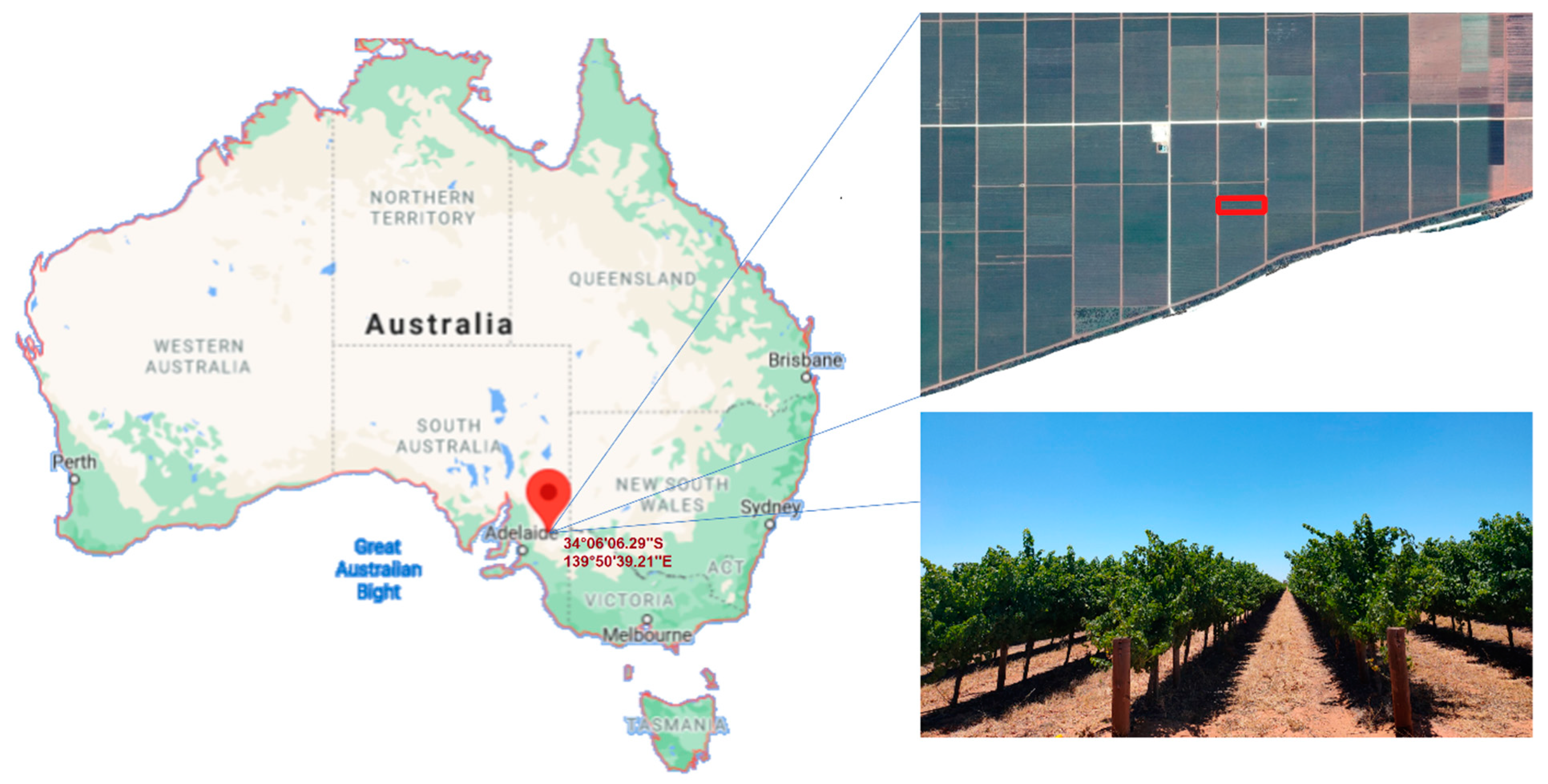
2.5.2. Optimum Hyperspectral Reflectance Bands Selection

The selection of the wavebands was based on the premise that the optimum bands are those that have the lowest autocorrelation, provide high information, and allow discrimination of the target [59,60]. To quantify these three assumptions, the analysis was carried out as follows.
First, the spectral regions between 350–399 nm, 1355–1420 nm, 1810–1940 nm and 2470–2500 nm were removed from analysis. These regions are considered to be noisy regions [59,61]. Then, the spectral regions that are more sensitive to HS under different cooling treatments were identified by plotting the percentage reflectance of each treatment relative to that of SI+, which was expected to be the most effective treatment.
SWIR and NIR spectral regions were also analyzed, because small reflectance differences in these spectral regions may correspond to strong differences in plant vigor caused by signal saturation [62]. Thus, spectral regions with a wavelength before 720 nm (red edge) were selected considering those with higher differences, whereas spectral regions beyond the red edge were investigated even if smaller differences were detected, considering the highest reflectance of plants in those spectral regions.
The bands pertaining to the areas of different spectral regions which exhibited higher differences from SI+ in all the other treatments were selected for further analysis.
Then, a band–band regression model was used. A high coefficient of determination (R2) value between two bands implies redundant information, whereas a low R2 value indicates that the two bands contain unique information, and thus are not auto-correlated (i.e., have low collinearity). For each band of spectral region identified in the previous step, the band pair correlations with the lowest R2 were selected, leading to six band combinations. Principal component analysis (PCA) was carried out between the selected bands and the physiological parameters for each treatment. The PCA was implemented with the R statistical software (Version 3.5.2, RStudio Version 1.0.463) using the R package “FactoExtra” [63]. The aim was to analyze the importance of these bands for discriminating the different treatments. The band–band regression model was implemented with R statistical software, using the package “corrr” [64] and selecting the pairs with the lowest R2.
To identify useful bands, further PCA was carried out using all the wavebands identified with the percentage reflectance plot. The bands were plotted against E rates measured two days after the end of HS, which showed the highest correlation with the spectral information and higher variability within the treatments. The five highest contribution bands of three principal components (PCs) were selected. The PCA was performed using the R statistical software.
Finally, Discriminant Analysis (DA) was performed to test the strength of data in discriminating the treatments. Due to the collinearity of many bands, it was not possible to run DA on original data, and data transformation did not improve the analysis. Therefore, DA was performed on twelve bands identified by the first three PCs of PCA and showing a Pearson’s correlation coefficient lower than │0.700│ [65,66]. The DA was carried out using the R package “klaR” [67] and splitting the dataset into training (80%) and test (20%) data. Figure 2 shows the conceptual selection model.

3. Results

According to the AWS, on the 14 and 15 January 2020, the maximum temperature in the study area was above 35 °C. Although this could not be considered a heatwave, the vines experienced HS. When the air temperature exceeds 35 °C, key physiological processes of grapevines are compromised [68]. Detailed statistics on weather conditions that occurred on the 14th and 15th of January 2020 are reported in Table 2.

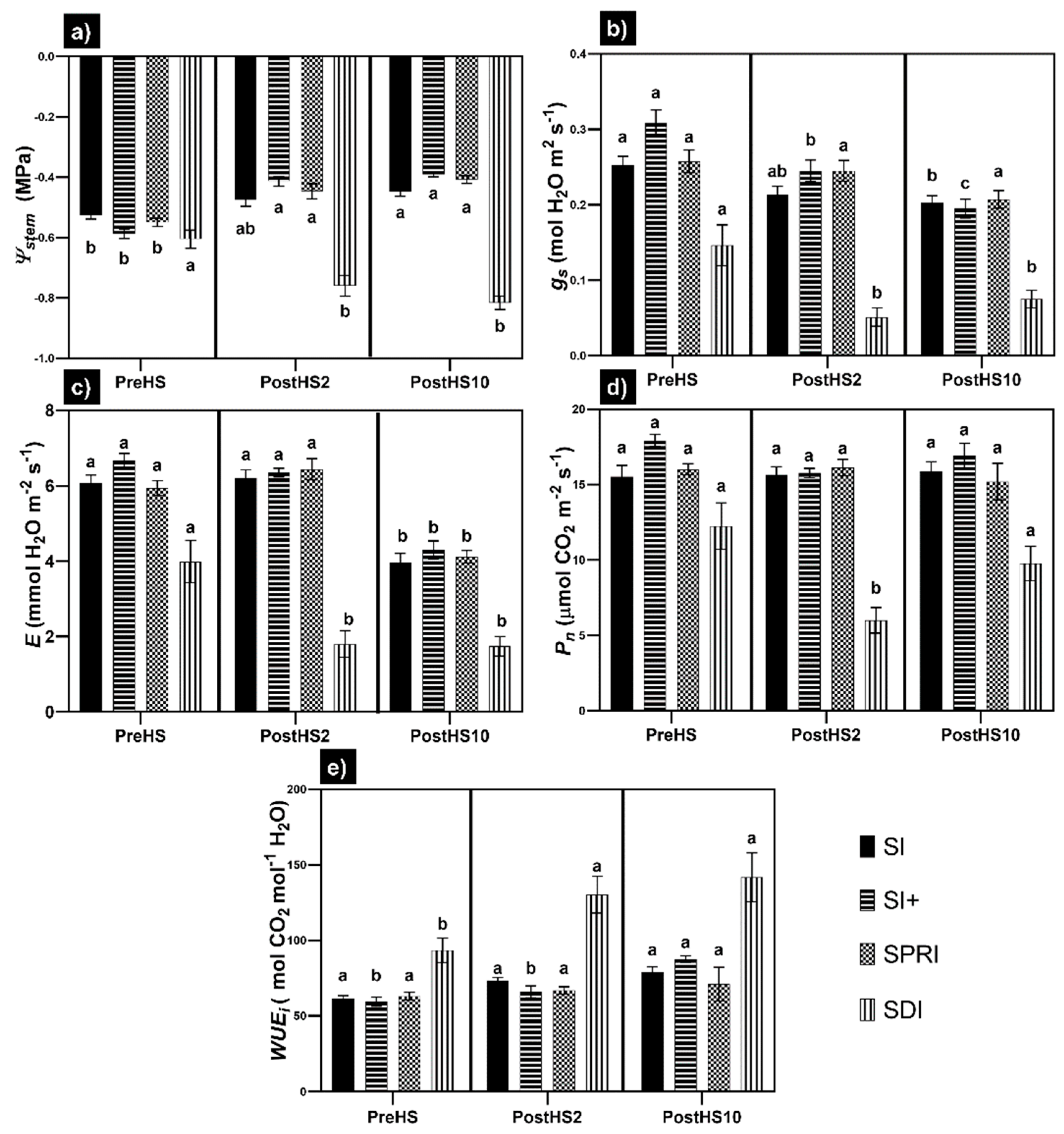
3.1. Grapevine Physiological Status: Water Relations and Gas Exchange

The physiological indicators of the treatments were compared using a two-way ANOVA (Figure 3).
Two days after the end of HS, Ψstem of two treatments (SI+ and SPRI) were higher than before HS (+29.7 and +25.8%, respectively). The same trend continued 10 days after the end of HS. SI did not show significantly different Ψstem values two days after the end of HS, but Ψstem significantly improved 10 days after the end of HS compared to the 10th of January, before HS (+14.7%). Ψstem of SDI showed a significant drop two days after the end of HS (−25.6%), which persisted 10 days after the end of HS (−34.8%).
The only treatment which maintained constant gs over time was SPRI. The values of gs did not show significant differences two days after the end of HS under SI but dropped after 10 days (−19.8% compared to before HS). SI+ showed a constant decrease in gs (−20.6% and −36.8% two and 10 days after the end of HS, respectively). Under SDI, gs dropped significantly two days after the end of HS (−65.0%), and, despite a slight recovery, stayed at a low level 10 days after the end of HS.
The trend of E was the same for three treatments (SI+, SPRI, and SI) with a significant decrease only 10 days after the end of HS. Conversely, E dropped in SDI immediately after HS (−54.8%), and the difference persisted 10 days after the end of HS.
Three treatments (SI+, SPRI, and SI) did not show any differences in Pn. Only SDI exhibited lower Pn rates two days after the end of HS (−51.0%) but recovered 10 days after the end of HS.
With regards to WUEi, SPRI and SI did not show any significant change after HS. WUEi was higher 10 days after the end of HS for SI+ (+47.8%). A significant increase was registered for SDI starting from two days after the end of HS (+39.5%) and persisted 10 days after the end of HS (+51.8%). Detailed information on the relative differences of the physiological parameters from the date before HS are reported in the Supplementary Materials (Table S1).

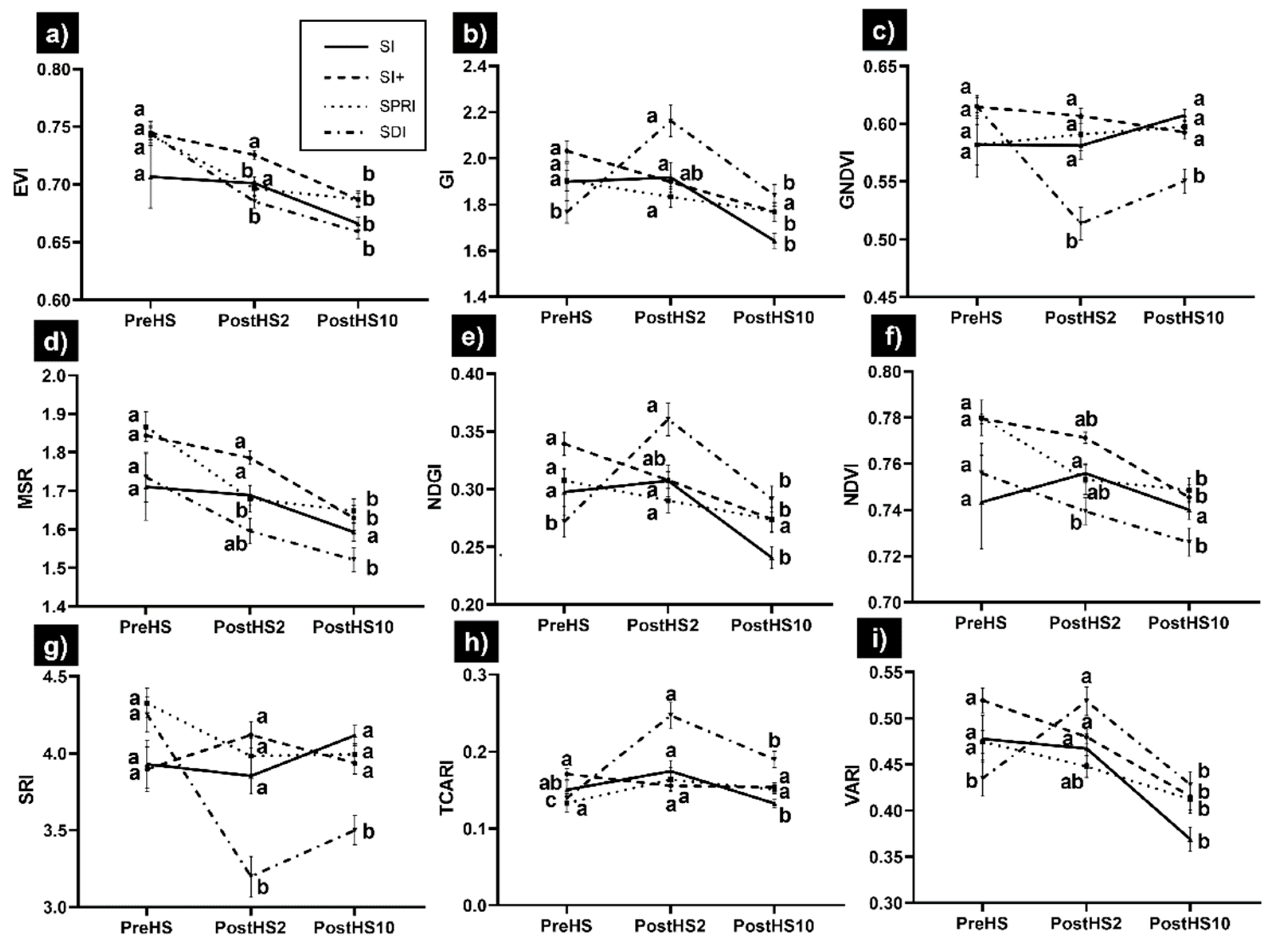
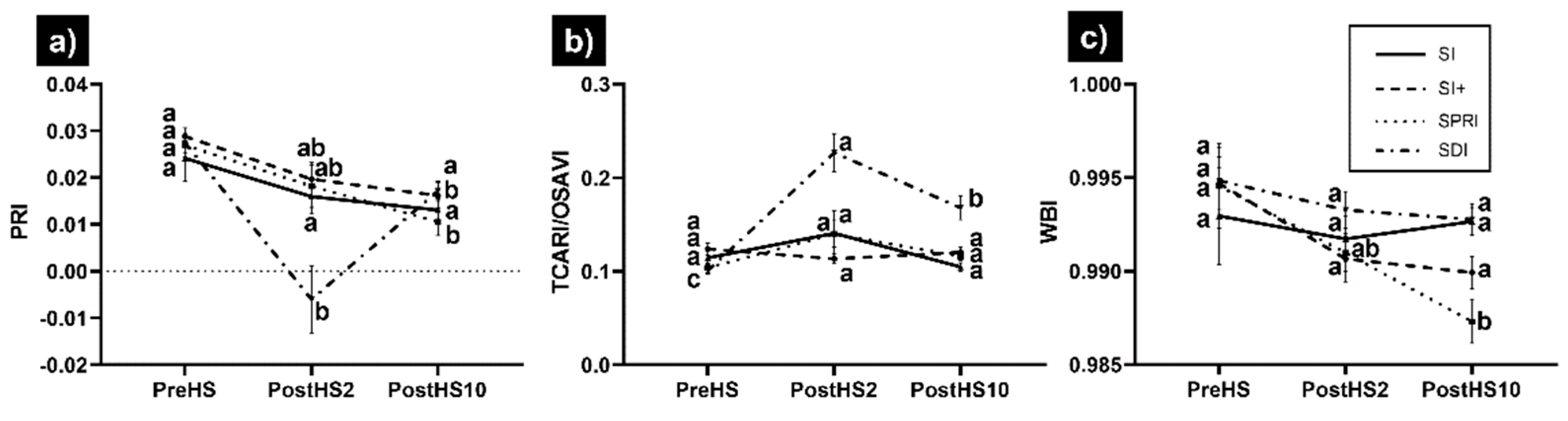
3.2. Hyperspectral-Derived VIs

With regards to the greenness VIs (Figure 4), in SI, EVI showed a significant difference 10 days after HS; GNDVI, MSR, NDVI, SRI, and TCARI were not affected by HS; GI, NDGI, and VARI showed a significant amelioration 10 days after HS. In SI+, EVI, MSR, and NDVI were significantly different 10 days after HS, but GI, GNDVI, NDGI, and VARI exhibited significant amelioration 10 days after HS. In SPRI, EVI, MSR, and NDVI showed a significant difference 10 days after HS, whereas GI, GNDVI, NDGI, SRI, and TCARI were not affected by HS. In SDI, most of the VIs exhibited lower performance immediately after HS, but GI and NDGI recovered 10 days after HS.
The remaining VIs showed different behavior (Figure 5). In SI, they did not show significant differences after HS. In SI+, PRI was significantly different from previous dates 10 days after the end of HS, whereas TCARI/OSAVI and WBI did not exhibit significant changes. In SPRI, PRI and WBI showed a significant difference 10 days after HS, and TCARI/OSAVI was not affected. In SDI, PRI was significantly lower two days after the end of HS and completely recovered 10 days after the end of HS; TCARI/OSAVI was significantly higher two days after the end of HS, with partial recovery 10 days after the end of HS; WBI showed a slight inflection immediately after HS, but was not significantly different from before HS. Subsequently, WBI started to recover. Detailed information on the relative differences in the VIs from the date before HS are reported in the Supplementary Materials (Table S2).

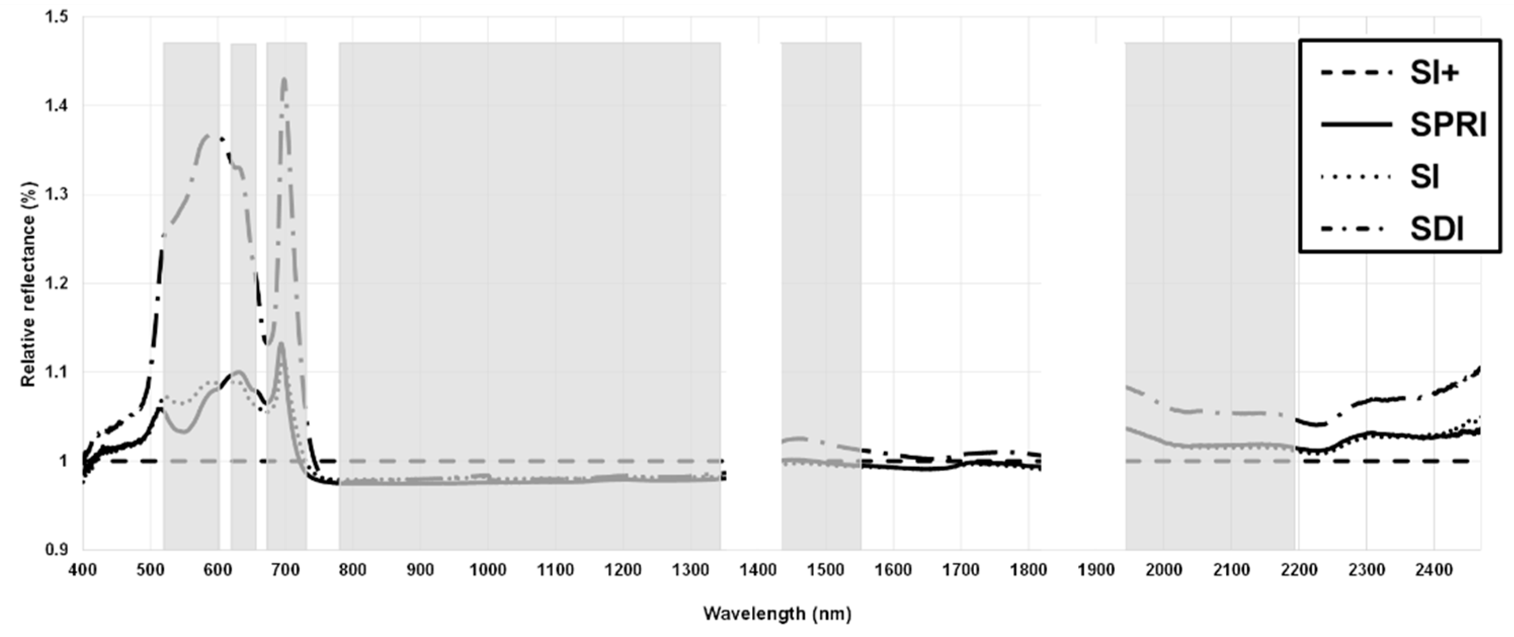
3.3. Optimum Bands Selection

The spectrum was filtered to identify the spectral regions more sensitive to HS, and the percentage reflectance of each treatment relative to that of SI+ was analyzed. The visual assessment allowed the selection of 520–610 nm (green), 620–640 nm (red), 680–720 nm (red edge), 770–1340 nm (NIR), 1421–1550 nm (SWIR), and 1941–2200 nm (water absorption bands) for further analysis (Figure 6).
The filtered bands were further investigated with a three-step process, including a band–band regression model, PCA, and DA. The band–band regression model revealed five pairs of bands that showed a very low coefficient of determination (0.001 ≤ R2 ≤ 0.203, p ≤ 0.05), thus providing unique information (Table 3). The most frequently occurring wavebands with low R2 in the correlation matrix included the wavelengths pertaining to NIR (770–1340 nm) and the water absorption bands (1941–2200 nm). However, the selection of the band pairs aimed to include all the spectral regions identified with the relative reflectance filtering process (Figure 6): green, red, red edge, NIR, SWIR, and water absorption bands. Therefore, once the pairs with the coefficient of determination within the aforementioned range were identified, some were excluded based on their redundancy (bands similar to other pairs). The examination of the lowest R2 bands with a PCA for each treatment allowed recognition of the best predictors of physiological status under HS (Figure 7). Overall, SI+, SDI, and SI performed similarly, with the water absorption bands (1496, 1948, 1952, and 2032 nm) negatively correlated with Pn, E, and gs due to their location in the opposite quadrant, and a second group of wavebands (570, 604, 636, 720, 1000, and 1033 nm) with a weaker correlation to the physiological parameters. However, in contrast to the positive correlation between Ψstem and water absorption bands in SI+, the correlation was negative for SDI and SI. Furthermore, in SPRI, not only Ψstem, but also gs had a positive correlation with water absorption bands and the red band (636 nm).
The second step for band selection was PCA, which aimed to reduce 1013 wavebands to 15 critical bands, and enabled identification of three main spectral regions. The results showed that PC1, PC2, and PC3 were dominated by bands pertaining to NIR, water absorption bands, and the transition region between green and red bands. The first five contributing bands for each PC are displayed in Table 4.
DA was inconclusive because it did not allow further discrimination between the twelve input variables. However, the twelve bands had reasonable potential to allow discrimination of the treatments (Wilk’s lambda = 0.47).

4. Discussion

Between December 2019 and January 2020, the study area suffered from repeated days of HS. We examined the HS days between the 14th and the 16th of January. During these days, the maximum temperature exceeded 35 °C for the first two days and remained high on the third day (Table 2). Temperature in excess of 35 °C compromises grapevine maximum Pn and gs rates [68,69]. Thus, we tested the potential of different cooling systems to counter HS and the spectral responses of the vines under combined WS and HS, because premium vineyards for wine grapes are often deficit irrigated.

4.1. Which Cooling Was the Most Effective in Mitigating HS?

SI, SI+, and SPRI were applied to counter HS. SI provided 6–7 ML ha−1 per season, which is typical of highly productive vineyards in this region. Based on whole canopy gas exchange measurements, these grapevines require approximately 40 L vine−1 day−1, whereas they were irrigated at approximately 20–25 L vine−1 day−1 [70]. By comparison, SI+ and SPRI proved to influence RH and reduce VPD inside the canopy without changing soil moisture [23]. The different levels of HS under different cooling systems were assessed by comparing physiological status indicators using ANOVA.
The results showed that SDI treatment suffered from HS, because all the physiological indicators were significantly lower two days after the end of HS, and the stress condition persisted 10 days after the end of HS (Figure 3). The analysis of Ψstem allowed for the quantitation of WS in SDI. Although the value of Ψstem before HS in SDI was not extremely low (−0.63 MPa ± 1.6 MPa), this value was significantly different from that of the other treatments. The value of Ψstem recorded in SDI was consistent with a WS condition during the post-fruit set stage [71]. Moreover, Ψstem further decreased after HS (Figure 3a), indicating the concurrence of WS in SDI. The overall decline experienced under HS, characterized by physiological parameters, indicates a water conservation response [72]. The closure of stomata to limit water losses is one of the first reactions to WS, thus decreasing gs and Ψstem. Stomatal control allows regulation of Pn and E, preserving vines from irreversible damage [73]. In the early phenological stages, the reduction in Ψstem induced by WS often coincides with reduced leaf area [74]. The limited photosynthetic area entails the decline in Pn. Furthermore, drought-induced closure of stomata is commonly associated with increased WUEi values. Therefore, Ψstem, Pn, E, gs, and WUEi are physiological traits commonly associated with WS.
The analysis of Ψstem (Figure 3a) proved that SI+ and SPRI, the treatments which were supplied with more water during HS days, improved their performance after HS. SI also showed a higher Ψstem 10 days after the end of HS. Ψstem is considered a reliable index of water status in Vitis vinifera, and its values are the combination of different factors, such as VPD, soil water availability, stomatal regulation, and plant hydraulic conductivity [75,76].
Many studies have found that Ψstem and E rates decrease after HS, whereas the findings related to gs behavior are controversial, because it is difficult to isolate the direct effect of temperature on gs [77,78,79]. In the current study, gs decreased significantly after HS, not only in SDI, but also in SI+ and SI, and persisted for up to 10 days after the end of the HS event (Figure 3b). In SPRI, gs did not exhibit significant variation after HS, thus leading to the conclusion that HS causes stomatal closure in Sauvignon blanc, and SPRI treatments did not undergo HS. Under HS conditions, E remained initially high for the evaporative cooling treatments, thereby maintaining a relatively constant canopy temperature via evaporative cooling, but dropped rapidly for SDI (Figure 3c), thus highlighting the severe effect of combined HS and WS [80,81]. However, all treatments showed lower E 10 days after HS, probably due to higher average RH. In agreement with the findings of Luo et al. [82], HS at 35 °C did not significantly inhibit Pn, with the exception of SDI (Figure 3d). HS results in a trade-off between hydraulic function and leaf temperature, i.e., opening stomata to transpire under HS may compromise hydraulics and generate WS, whereas closing stomata may increase the leaf temperature to the point that Pn drops off [83]. Moreover, during HS, light energy usually absorbed by chlorophyll for photochemistry is partially lost as sensible heat [84]. Furthermore, there is a build-up of toxic reactive oxygen species inside the photochemical apparatus of the leaves, which can be quenched by heat dissipation mechanisms such as non-photochemical quenching. Finally, HS induces the biosynthesis of heat stress proteins (HSPs), which represents a vital adaptative mechanism. Nevertheless, the energy spent by the vines for the synthesis of HSPs has negative repercussions on yield [85]. The significant decrease in Pn only in SDI may confirm the potential efficiency of cooling systems in the other treatments.
According to the primary studies on grapevines under HS conditions, Pn, gs, E, and Ψstem decreased sharply [24,78,86]. In this study, only SDI showed a decreasing trend for all of the former physiological parameters, whereas SI+ and SPRI showed higher Ψstem. This response may confirm that the evaporative cooling systems had a positive effect on the mitigation of HS effects, with SPRI and SI+ performing slightly better than SI. Therefore, the cooling systems evaluated in this study may represent effective tools to counteract the negative influence of the heatwaves on vine physiological performance.

4.2. Which Is the Spectral Behavior of the Vines under Combined WS and HS?

Overall, the behavior of the VIs confirmed from the spectral perspective the observations in the physiological parameters (Figure 5 and Figure 6).
Two days after the end of HS, SDI significantly differed both from pre-HS and from the cooling treatments. An exception was WBI, which was not capable of combined stress in SDI (Figure 5c). Because changes in leaf water content only occur during late stages of dehydration [87], the failure of WBI to detect vines stress suggests that the vines experienced moderate WS, and that WBI can be excluded from VIs for early tracking of combined stress. The analysis of the percentage difference in physiological parameters and VIs two and 10 days after the end of HS (see Supplementary Materials) allowed the identification of some trends. Specifically, GI, NDGI, and VARI showed that HS affected only the SDI treatment, but their values recovered to initial (pre-HS) levels within 10 days after the end of HS. Concurrently, SI+ and SI treatments showed an improvement 10 days after the end of HS, which may be related to their cooling efficacies. GI, NDGI, and VARI are greenness indices, which combine the green and red bands to account for dry vegetation, and have been proven to be effective for estimating drought stress [88] and leaf water potential [89]. In this study, the performance of GI, NDGI, and VARI was consistent with that of Ψstem and Pn. The spectral bands included in the equation of these VIs pertain to the visible domain, whose reflectance is influenced by pigment content [51]. The pigment content is related to HS, i.e., increased carotenoids and decreased Chlorophyll a and b content [90]. Therefore, the findings of this study suggest that the evaporative cooling systems mitigated physiological stresses associated with HS. In comparison, SRI, TCARI, and TCARI/OSAVI revealed a slightly different situation, with SDI still declining soon after HS, but not recovering even 10 days after the end of HS. Concurrently, the other treatments did not exhibit any significant change. Compared with the previous group of VIs, the VIs belonging to this second group contain the NIR (SRI) and/or red edge (TCARI and TCARI/OSAVI) bands. The reduction in water content after WS leads to a decreased NIR reflection. In previous studies, SRI has been used to assess vineyard water status [37,41]. Moreover, NIR has been previously shown to discriminate HS and estimate E [3]. VIs calculated in the red-edge spectral region were even more sensitive than NIR in the identification of temperature- and water-induced changes in Cabernet Sauvignon [91]. The failure of recovery of these VIs may indicate that, despite greenness and vigor amelioration, the physiological parameters could not recover as quickly after the combination of HS and WS. This hypothesis was supported by the fact that Pn and WUEi showed the same trend as SRI, TCARI, and TCARI/OSAVI (Supplementary Materials). The third group of VIs (MSR, NDVI, and EVI) yielded slightly different and heterogeneous results, yet captured the effect of HS on SDI. Indices of the latter group result from a combination of red and NIR bands. Previous studies showed a difference of less than 1.0% in red reflectance for grapevines under HS conditions [91]. Our results suggest that VIs containing a combination of green, NIR, and red edge bands may help to track combined WS and HS in grapevines.
The three-step band selection process (band–band regression, PCA, and DA) aimed at providing complementary information by eliminating redundant bands (band–band regression and PCA), identifying the bands which drive vine response to WS and HS (PCA), and highlighting the bands which discriminate the treatment (DA). The first three PCs of PCA (Table 4) showed that the spectral regions involved in the vine response to HS were NIR (1336–1340 nm), water absorption bands (1967–1971 nm), and the transition region between green and red bands (600–604 nm). Compared to SI+, the other treatments responded to HS by increasing the reflectance in the green/red and NIR regions, while decreasing it in the region of the water absorption bands (Figure 5). The 550–680 nm and red-edge bands are indicators of chlorophyll content at the leaf level [84,92]. The reflectance in the spectral region around 1240–1450 nm is influenced by leaf water content [93,94]. Consistent with the VI analysis, our findings indicate that two physiological processes—Pn and E—show the highest sensitivity to HS.
Band–band regression allowed for the determination of specific bands within each spectral region, which provided meaningful information about HS (Table 3). Some of the information provided by band–band regression was confirmed by PCA. Specifically, bands 604, 720, and 1333–1340 nm were recurrent in both analyses. Bands 1496, 1948, 1952, and 2032 nm showed a strong inverse correlation with Pn and E for all treatments, whereas gs was directly correlated with these bands for SPRI and inversely correlated for the other treatments. Some of the aforementioned bands (604, 1496, 1948, and 1952 nm) are known to be sensitive to leaf water content [28,95,96]. Another difference indicated by the PCA of the lowest correlation bands was the direct correlation of bands 1000 and 1333 nm with the physiological indicators—Ψstem, gs, Pn, and E—for SDI (Figure 7b). This finding suggests that NIR is the critical spectral region for detection of the combined effects of HS and WS.

5. Conclusions

In this study, we analyzed the physiological behavior of Sauvignon blanc under conditions of individual HS and combined HS and WS. Moreover, we compared the effectiveness of different evaporative cooling systems to mitigate HS. Finally, we tested the hypothesis that hyperspectral reflectance and derived VIs can provide effective and valuable information on grapevine response to HS conditions, and in combination with WS. Our main findings were:
  • Combined HS and WS led to unsatisfactory Ψstem, gs, Pn, E, and WUEi values, which did not recover within 10 days.
  • The cooling systems evaluated in the present study were efficacious in mitigating the adverse effects of HS. Specifically, SI+ and SPRI exhibited higher Ψstem after HS. Moreover, in SI+, Pn was not affected by HS in cooled vines, and in SPRI, both Pn and gs were unaffected.
  • The spectral VIs showed that SI+, SPRI, and SI were rapidly able to recover the greenness and vigor, as shown by GI, NDGI, and VARI.
  • The vine physiological function did not completely recover even 10 days after HS with SRI, TCARI, and TCARI/OSAVI significantly different than their values before HS. The lack of full recovery may indicate that the VIs were sensitive to changes in gs.
  • The spectral regions more sensitive to HS were NIR (770–1340 nm), water absorption bands (1941–2200 nm), and the transition region between the green and red bands (600–604 nm), with NIR having the ability to discriminate between SDI and the cooling treatments.
  • The single wavebands most sensitive to HS were 604, 720, and 1333–1340 nm.
  • The hyperspectral data were consistent with physiological data, identifying SDI as the worst-performing treatment under HS, and SI+ and SPRI as effective cooling strategies to cope with HS.
In the current climate change context, vineyards are likely to increasingly experience HS, and farmers need to be supported with managing strategies. Scientific research has yet to devote sufficient attention to the effects of HS, and combined HS and WS, on vineyards. The physiological behavior of grapevines under HS still needs to be determined, and further study will be needed on different varieties, conditions, and areas before obtaining a comprehensive understanding of the topic. The measurement of physiological parameters with conventional methods is time consuming and tedious, particularly during hot days. The opportunity to replace these measurements with spectral assessments, either from proximal or remote instrumentation, would represent an effective and rapid tool to monitor environmental stresses in the field. Therefore, the findings and the methodology proposed in this study contribute to expanding the knowledge of the effects of HS, and combined HS and WS, and the tools for future investigation.
Moreover, we explored the effectiveness of different evaporative cooling systems to help farmers cope with the adverse effects of HS. The findings may promote the implementation of vineyard irrigation strategies to ensure sustainable and profitable production.

Supplementary Materials

The following are available online at https://www.mdpi.com/article/10.3390/agronomy11101940/s1, Table S1: Differences in physiological parameters compared to the values before HS. Single asterisk indicates a significant difference, p < 0.05; double asterisk indicates a statistical difference, p < 0.01; triple asterisk indicates a statistical difference, p < 0.001; ns indicates no significant difference (p > 0.05), Table S2: Differences in VIs compared to the values before HS. Single asterisk indicates a significant difference, p < 0.05; double asterisk indicates a statistical difference, p < 0.01; triple asterisk indicates a statistical difference, p < 0.001; ns indicates no significant difference (p > 0.05).

Author Contributions

Conceptualization, A.C. and V.P.; methodology, A.C., V.P.; software, A.C., V.P. and S.Y.Y.J.; validation, F.M. (Francesco Marinello) and F.M. (Franco Meggio); formal analysis, A.C., S.Y.Y.J. and L.W.; investigation, A.C., S.Y.Y.J. and L.W.; data curation, A.C. and L.W.; writing—original draft preparation, A.C.; writing—review and editing, A.C., V.P., F.M. (Francesco Marinello), F.M. (Franco Meggio), M.S. and S.Y.Y.J.; supervision, V.P. All authors have read and agreed to the published version of the manuscript.

Funding

This research received no external funding.

Data Availability Statement

All the data generated or analyzed during this study are included in this published editorial.

Acknowledgments

The authors would like to thank Yalumba Oxford Landing Estate for providing the trial site and for vineyard management.

Conflicts of Interest

The authors declare no conflict of interest.

References

  1. Arneth, A.; Barbosa, H.; Benton, T.; Calvin, K.; Calvo, E.; Connors, S. Summary for policymakers. In Climate Change and Land: 602 an Ipcc Special Report on Climate Change, Desertification, Land Degradation, Sustainable Land Management, Food Security, and Greenhouse Gas Fluxes in Terrestrial Ecosystems; IPCC: Geneva, Swizerland, 2019. [Google Scholar]
  2. Perkins-Kirkpatrick, S.; Pitman, A. Extreme events in the context of climate change. Public Health Res. Pract. 2018, 28, 2–5. [Google Scholar] [CrossRef] [Green Version]
  3. Cogato, A.; Pagay, V.; Marinello, F.; Meggio, F.; Grace, P.; Migliorati, M.D.A. Assessing the feasibility of using Sentinel-2 imagery to quantify the impact of heatwaves on irrigated vineyards. Remote Sens. 2019, 11, 2869. [Google Scholar] [CrossRef] [Green Version]
  4. Bucur, G.M.; Babes, A.C. Research on trends in extreme weather conditions and their effects on grapevine in Romanian viticulture. Bull. UASVM Hortic. 2016, 73, 126–134. [Google Scholar]
  5. Duchêne, E.; Huard, F.; Dumas, V.; Schneider, C.; Merdinoglu, D. The challenge of adapting grapevine varieties to climate change. Clim. Res. 2010, 41, 193–204. [Google Scholar] [CrossRef] [Green Version]
  6. Carvalho, L.; Coito, J.L.; Gonçalves, E.M.F.; Chaves, M.M.; Amâncio, S. Differential physiological response of the grapevine varieties Touriga Nacional and Trincadeira to combined heat, drought and light stresses. Plant Biol. 2015, 18, 101–111. [Google Scholar] [CrossRef] [PubMed]
  7. Greer, D.H.; Weedon, M.M. The impact of high temperatures on vitis vinifera cv. semillon grapevine performance and berry ripening. Front. Plant Sci. 2013, 4, 1–9. [Google Scholar] [CrossRef] [Green Version]
  8. Liang, L.; Sun, Q.; Luo, X.; Wang, J.; Zhang, L.; Deng, M.; Di, L.; Liu, Z. Long-term spatial and temporal variations of vegetative drought based on vegetation condition index in China. Ecosphere 2017, 8, e01919. [Google Scholar] [CrossRef]
  9. Cowan, T.; Purich, A.; Perkins-Kirkpatrick, S.; Pezza, A.; Boschat, G.; Sadler, K. More Frequent, Longer, and Hotter Heat Waves for Australia in the Twenty-First Century. J. Clim. 2014, 27, 5851–5871. [Google Scholar] [CrossRef]
  10. Schoetter, R.; Cattiaux, J.; Douville, H. Changes of western European heat wave characteristics projected by the CMIP5 ensemble. Clim. Dyn. 2014, 45, 1601–1616. [Google Scholar] [CrossRef]
  11. Chaves, M.M.; Zarrouk, O.; Francisco, R.; Costa, J.M.; Santos, T.; Regalado, A.P.; Rodrigues, M.L.; Lopes, C.M. Grapevine under deficit irrigation: Hints from physiological and molecular data. Ann. Bot. 2010, 105, 661–676. [Google Scholar] [CrossRef] [Green Version]
  12. Bonada, M.; Sadras, V.; Fuentes, S. Effect of elevated temperature on the onset and rate of mesocarp cell death in berries of Shiraz and Chardonnay and its relationship with berry shrivel. Aust. J. Grape Wine Res. 2013, 19, 87–94. [Google Scholar] [CrossRef]
  13. Xiao, Z.; Liao, S.; Rogiers, S.; Sadras, V.; Tyerman, S. Effect of water stress and elevated temperature on hypoxia and cell death in the mesocarp of Shiraz berries. Aust. J. Grape Wine Res. 2018, 24, 487–497. [Google Scholar] [CrossRef]
  14. Sadras, V.; Moran, M.; Bonada, M. Effects of elevated temperature in grapevine. I Berry sensory traits. Aust. J. Grape Wine Res. 2012, 19, 95–106. [Google Scholar] [CrossRef]
  15. Zhang, P.; Howell, K.; Krstic, M.; Herderich, M.; Barlow, E.W.R.; Fuentes, S. Environmental factors and seasonality affect the concentration of rotundone in Vitis vinifera L. cv. Shiraz wine. PLoS ONE 2015, 10, e0133137. [Google Scholar] [CrossRef] [PubMed] [Green Version]
  16. Rashid, M.A.; Andersen, M.N.; Wollenweber, B.; Kørup, K.; Zhang, X.; Olesen, J.E. Impact of heat-wave at high and low VPD on photosynthetic components of wheat and their recovery. Environ. Exp. Bot. 2018, 147, 138–146. [Google Scholar] [CrossRef]
  17. Bhusal, N.; Han, S.-G.; Yoon, T.-M. Impact of drought stress on photosynthetic response, leaf water potential, and stem sap flow in two cultivars of bi-leader apple trees (Malus × domestica Borkh.). Sci. Hortic. 2019, 246, 535–543. [Google Scholar] [CrossRef]
  18. Gambetta, G.A.; Herrera, J.C.; Dayer, S.; Feng, Q.; Hochberg, U.; Castellarin, S.D. The physiology of drought stress in grapevine: Towards an integrative definition of drought tolerance. J. Exp. Bot. 2020, 71, 4658–4676. [Google Scholar] [CrossRef]
  19. Min, Z.; Li, R.; Chen, L.; Zhang, Y.; Li, Z.; Liu, M.; Ju, Y.; Fang, Y. Alleviation of drought stress in grapevine by foliar-applied strigolactones. Plant Physiol. Biochem. 2019, 135, 99–110. [Google Scholar] [CrossRef]
  20. Mittler, R. Abiotic stress, the field environment and stress combination. Trends Plant Sci. 2006, 11, 15–19. [Google Scholar] [CrossRef]
  21. Jing, B.; Shah, F.; Xiao, E.; Coulter, J.A.; Wu, W. Sprinkler irrigation increases grain yield of sunflower without enhancing the risk of root lodging in a dry semi-humid region. Agric. Water Manag. 2020, 239, 106270. [Google Scholar] [CrossRef]
  22. Gilbert, D.E.; Meyer, J.L.; Kissler, J.J.; La Vine, P.D.; Carlson, C.V. Evaporation cooling of vineyards. Calif. Agric. 1970, 24, 12–14. [Google Scholar] [CrossRef] [Green Version]
  23. Pagay, V.; Tyerman, S.; Jeffery, D.; Muhlack, R.; McCarthy, M.; Boss, P. Using in-Canopy Misters to Mitigate the Negative Effects of Heatwaves in Grapevines; Final Report to Wine Australia; 2018; Available online: https://www.wineaustralia.com/research/projects/using-in-canopy-misters-to-mitigate-the (accessed on 10 September 2021).
  24. Edwards, E.; Smithson, L.; Graham, D.; Clingeleffer, P. Grapevine canopy response to a high-temperature event during deficit irrigation. Aust. J. Grape Wine Res. 2011, 17, 153–161. [Google Scholar] [CrossRef]
  25. Sousa, T.A.; Oliveira, M.T.; Moutinho-Pereira, J. Physiological indicators of plant water status of irrigated and non-irrigated grapevines grown in a low rainfall area of portugal. Plant Soil 2006, 282, 127–134. [Google Scholar] [CrossRef]
  26. Girona, J.; Mata, M.; del Campo, J.; Arbonés, A.; Bartra, E.; Marsal, J. The use of midday leaf water potential for scheduling deficit irrigation in vineyards. Irrig. Sci. 2006, 24, 115–127. [Google Scholar] [CrossRef]
  27. Cogato, A.; Meggio, F.; Collins, C.; Marinello, F. Medium-resolution multispectral data from Sentinel-2 to assess the damage and the recovery time of late frost on vineyards. Remote Sens. 2020, 12, 1896. [Google Scholar] [CrossRef]
  28. Poblete, T.; Ortega-Farías, S.; Moreno, M.A.; Bardeen, M. Artificial neural network to predict vine water status spatial variability using multispectral information obtained from an unmanned aerial vehicle (UAV). Sensors 2017, 17, 2488. [Google Scholar] [CrossRef] [Green Version]
  29. Zarco-Tejada, P.J.; Ustin, S.; Whiting, M.L. Temporal and spatial relationships between within-field yield variability in cotton and high-spatial hyperspectral remote sensing imagery. Agron. J. 2005, 97, 641–653. [Google Scholar] [CrossRef] [Green Version]
  30. Cogato, A.; Pezzuolo, A.; Sørensen, C.G.; De Bei, R.; Sozzi, M.; Marinello, F. A GIS-based multicriteria index to evaluate the mechanisability potential of Italian vineyard area. Land 2020, 9, 469. [Google Scholar] [CrossRef]
  31. Mirás-Avalos, J.M.; Pérez-Sarmiento, F.; Alcobendas, R.; Alarcón, J.J.; Mounzer, O.; Nicolás, E. Using midday stem water potential for scheduling deficit irrigation in mid–late maturing peach trees under Mediterranean conditions. Irrig. Sci. 2016, 34, 161–173. [Google Scholar] [CrossRef]
  32. Choné, X.; Van Leeuwen, C.; Dubourdieu, D.; Gaudillère, J.P. Stem water potential is a sensitive indicator of grapevine water status. Ann. Bot. 2001, 87, 477–483. [Google Scholar] [CrossRef] [Green Version]
  33. Prieto, J.A.; Lebon, É.; Ojeda, H. Stomatal behavior of different grapevine cultivars in response to soil water status and air water vapor pressure deficit. J. Int. Sci. Vigne Vin 2010, 44, 9–20. [Google Scholar] [CrossRef]
  34. Santesteban, L.G.; Miranda, C.; Royo, J.B. Effect of water deficit and rewatering on leaf gas exchange and transpiration decline of excised leaves of four grapevine (Vitis vinifera L.) cultivars. Sci. Hortic. 2009, 121, 434–439. [Google Scholar] [CrossRef]
  35. Tomás, M.; Medrano, H.; Escalona, J.M.; Martorell, S.; Pou, A.; Ribas-Carbo, M.; Flexas, J. Variability of water use efficiency in grapevines. Environ. Exp. Bot. 2014, 103, 148–157. [Google Scholar] [CrossRef]
  36. Greer, D.H.; Weston, C. Heat stress affects flowering, berry growth, sugar accumulation and photosynthesis of Vitis vinifera cv. Semillon grapevines grown in a controlled environment. Funct. Plant Biol. 2010, 37, 206–214. [Google Scholar] [CrossRef]
  37. Zarco-Tejada, P.J.; Berjón, A.; López-Lozano, R.; Miller, J.R.; Martín, P.; Cachorro, V.; González, M.R.; De Frutos, A. Assessing vineyard condition with hyperspectral indices: Leaf and canopy reflectance simulation in a row-structured discontinuous canopy. Remote Sens. Environ. 2005, 99, 271–287. [Google Scholar] [CrossRef]
  38. Rouse, J.; Haas, R.; Schell, J.; Deering, D.; Harlan, J. Monitoring the Vernal Advancement and Retrogradation (Greenwave Effect) of Natural Vegetation; Type III Final Report; NASA/GSFC: Greenbelt, MD, USA, 1974; p. 371.
  39. Acevedo-Opazo, C.; Tisseyre, B.; Guillaume, S.; Ojeda, H. Test of NDVI information for a relevant vineyard zoning related to vine water status. In Proceedings of the VI European Conference on Precision Agriculture (ECPA), Skiathos, Greece, 3–6 June 2007; pp. 547–554. [Google Scholar]
  40. Acevedo-Opazo, C.; Tisseyre, B.; Guillaume, S.; Ojeda, H. The potential of high spatial resolution information to define within-vineyard zones related to vine water status. Precis. Agric. 2008, 9, 285–302. [Google Scholar] [CrossRef] [Green Version]
  41. Baluja, J.; Diago, M.P.; Balda, P.; Zorer, R.; Meggio, F.; Morales, F.; Tardaguila, J. Assessment of vineyard water status variability by thermal and multispectral imagery using an unmanned aerial vehicle (UAV). Irrig. Sci. 2012, 30, 511–522. [Google Scholar] [CrossRef]
  42. Espinoza, C.Z.; Khot, L.R.; Sankaran, S.; Jacoby, P.W. High resolution multispectral and thermal remote sensing-based water stress assessment in subsurface irrigated grapevines. Remote Sens. 2017, 9, 961. [Google Scholar] [CrossRef] [Green Version]
  43. Serrano, L.; González-Flor, C.; Gorchs, G. Assessing vineyard water status using the reflectance based Water Index. Agric. Ecosyst. Environ. 2010, 139, 490–499. [Google Scholar] [CrossRef]
  44. Zarco-Tejada, P.J.; Gonzalez-Dugo, V.; Williams, L.; Suárez, L.; Jimenez-Berni, J.A.; Goldhamer, D.; Fereres, E. A PRI-based water stress index combining structural and chlorophyll effects: Assessment using diurnal narrow-band airborne imagery and the CWSI thermal index. Remote Sens. Environ. 2013, 138, 38–50. [Google Scholar] [CrossRef]
  45. Di Gennaro, S.F.; Matese, A.; Gioli, B.; Toscano, P.; Zaldei, A.; Palliotti, A.; Genesio, L. Multisensor approach to assess vineyard thermal dynamics combining high-resolution unmanned aerial vehicle (UAV) remote sensing and wireless sensor network (WSN) proximal sensing. Sci. Hortic. 2017, 221, 83–87. [Google Scholar] [CrossRef]
  46. Gitelson, A.A.; Viña, A.; Ciganda, V.; Rundquist, D.C.; Arkebauer, T.J. Remote estimation of canopy chlorophyll content in crops. Geophys. Res. Lett. 2005, 32, 1–4. [Google Scholar] [CrossRef] [Green Version]
  47. Chen, J.M. Evaluation of vegetation indices and a modified simple ratio for boreal applications. Can. J. Remote Sens. 1996, 22, 229–242. [Google Scholar] [CrossRef]
  48. Haboudane, D.; Miller, J.R.; Tremblay, N.; Zarco-Tejada, P.J.; Dextraze, L. Integrated narrow-band vegetation indices for prediction of crop chlorophyll content for application to precision agriculture. Remote Sens. Environ. 2002, 81, 416–426. [Google Scholar] [CrossRef]
  49. Courel, M.-F.; Chamard, P.; Guenegou, M.J.; Lerhun, J.; Levasseur, M.; Togola, M. Utilisation des bandes spectrales du vert et du rouge pour une meilleure évaluation des formations végétales actives. In Proceedings of the Congrès AUPELF-UREF, Sherbrooke, QC, Canada, 21–23 October 1991; pp. 203–210. [Google Scholar]
  50. Jordan, C.F. Derivation of leaf-area index from quality of light on the forest floor. Ecology 1969, 50, 663–666. [Google Scholar] [CrossRef]
  51. Gitelson, A.A.; Kaufman, Y.J.; Stark, R.; Rundquist, D. Novel algorithms for remote estimation of vegetation fraction. Remote Sens. Environ. 2002, 80, 76–87. [Google Scholar] [CrossRef] [Green Version]
  52. Pôças, I.; Rodrigues, A.; Gonçalves, S.; Costa, P.M.; Gonçalves, I.; Pereira, L.S.; Cunha, M. Predicting grapevine water status based on hyperspectral reflectance vegetation indices. Remote Sens. 2015, 7, 16460–16479. [Google Scholar] [CrossRef] [Green Version]
  53. Gamon, J.A.; Peñuelas, J.; Field, C.B. A narrow-waveband spectral index that tracks diurnal changes in photosynthetic efficiency. Remote Sens. Environ. 1992, 41, 35–44. [Google Scholar] [CrossRef]
  54. Liu, H.Q.; Huete, A. A feedback based modification of the NDVI to minimize canopy background and atmospheric noise. IEEE Trans. Geosci. Remote Sens. 1995, 33, 457–465. [Google Scholar] [CrossRef]
  55. Cheng, Y.-B.; Zarco-Tejada, P.J.; Riano, D.; Rueda, C.A.; Ustin, S. Estimating vegetation water content with hyperspectral data for different canopy scenarios: Relationships between AVIRIS and MODIS indexes. Remote Sens. Environ. 2006, 105, 354–366. [Google Scholar] [CrossRef]
  56. Dold, C.; Heitman, J.; Giese, G.; Howard, A.; Havlin, J.; Sauer, T. Upscaling Evapotranspiration with parsimonious models in a North Carolina vineyard. Agronomy 2019, 9, 152. [Google Scholar] [CrossRef] [Green Version]
  57. Penuelas, J.; Filella, I.; Biel, C.; Serrano, L.; Savé, R. The reflectance at the 950–970 nm region as an indicator of plant water status. Int. J. Remote Sens. 1993, 14, 1887–1905. [Google Scholar] [CrossRef]
  58. Fórián, T.; Nagy, A.; Riczu, P.; Mézes, L.; Tamás, J. Vineyards characteristic by using GIS and refl ectance measurements on the Nagy-Eged hill in Hungary. Int. J. Hortic. Sci. 2016, 18, 57–60. [Google Scholar] [CrossRef] [Green Version]
  59. Thenkabail, P.S.; Enclona, E.A.; Ashton, M.S.; Van Der Meer, B. Accuracy assessments of hyperspectral waveband performance for vegetation analysis applications. Remote Sens. Environ. 2004, 91, 354–376. [Google Scholar] [CrossRef]
  60. Ray, S.S.; Singh, J.P.; Panigraphy, S. Use of hyperstectralremote senings data for crop stress detection: Ground-based studies. Int. Arch. Photogramm. Remote. Sens. Spat. Inf. Sci. 2010, 38, 562–570. [Google Scholar]
  61. Mutanga, O.; Skidmore, A.; Prins, H. Predicting in situ pasture quality in the Kruger National Park, South Africa, using continuum-removed absorption features. Remote Sens. Environ. 2004, 89, 393–408. [Google Scholar] [CrossRef]
  62. Huete, A.R.; Liu, H.Q.; van Leeuwen, W.J.D. The use of vegetation indices in forested regions: Issues of linearity and saturation. Int. Geosci. Remote Sens. Symp. 1997, 4, 1966–1968. [Google Scholar]
  63. Kassambara, A.; Mundt, F. Factoextra: Extract and Visualize the Results of Multivariate Data Analyses (Versión 1.0.5). Available online: https://cran.r-project.org/package=factoextra (accessed on 1 March 2021).
  64. Ruiz, E.; Jackson, S.; Cimentada, J. Corrr: Correlations in R. Available online: https://cran.r-project.org/web/packages/corrr/index.htm (accessed on 1 March 2021).
  65. Dormann, C.F.; Elith, J.; Bacher, S.; Buchmann, C.; Carl, G.; Carré, G.; Marquéz, J.R.G.; Gruber, B.; Lafourcade, B.; Leitão, P.J.; et al. Collinearity: A review of methods to deal with it and a simulation study evaluating their performance. Ecography 2013, 36, 27–46. [Google Scholar] [CrossRef]
  66. Yang, J.; Yang, J.Y. Why can LDA be performed in PCA transformed space? Pattern Recognit. 2003, 36, 563–566. [Google Scholar] [CrossRef]
  67. Roever, C.; Raabe, N.; Luebke, K.; Ligges, U.; Szepannek, G.; Zentgraf, M. klaR: Classification and visualization. Available online: https://cran.r-project.org/package=klaR (accessed on 1 March 2021).
  68. Greer, D.H.; Weedon, M. Modelling photosynthetic responses to temperature of grapevine (Vitis vinifera cv. Semillon) leaves on vines grown in a hot climate. Plant Cell Environ. 2011, 35, 1050–1064. [Google Scholar] [CrossRef]
  69. Zsófi, Z.; Gál, L.; Szilágyi, Z.; Szűcs, E.; Marschall, M.; Nagy, Z.; Bálo, B. Use of stomatal conductance and pre-dawn water potential to classify terroir for the grape variety Kékfrankos. Aust. J. Grape Wine Res. 2009, 15, 36–47. [Google Scholar] [CrossRef]
  70. Pagay, V.; Canela, F.; Bennet, C. How Does Phenological Stage Influence Grapevine Water Requirements for Shiraz and Chardonnay in the Riverland? Final Report to Wine Australia; 2021; Available online: https://www.growag.com/listings/research-project/incubator-initiative-how-does-phenological-stage-influence-grapevine-water-requirements-for-shiraz-and-chardonnay-in-the-riverland (accessed on 10 September 2021).
  71. Acevedo-Opazo, C.; Ortega-Farias, S.; Fuentes, S. Effects of grapevine (Vitis vinifera L.) water status on water consumption, vegetative growth and grape quality: An irrigation scheduling application to achieve regulated deficit irrigation. Agric. Water Manag. 2010, 97, 956–964. [Google Scholar] [CrossRef]
  72. Pierantozzi, P.; Torres, M.; Bodoira, R.; Maestri, D. Water relations, biochemical–physiological and yield responses of olive trees (Olea europaea L. cvs. Arbequina and Manzanilla) under drought stress during the pre-flowering and flowering period. Agric. Water Manag. 2013, 125, 13–25. [Google Scholar] [CrossRef]
  73. Bhusal, N.; Lee, M.; Lee, H.; Adhikari, A.; Han, A.R.; Kim, H.S. Evaluation of morphological, physiological, and biochemical traits for assessing drought resistance in eleven tree species. Sci. Total. Environ. 2021, 779, 146466. [Google Scholar] [CrossRef] [PubMed]
  74. Brito, C.; Dinis, L.-T.; Moutinho-Pereira, J.; Correia, C.M.; Pereira, M. Drought stress effects and olive tree acclimation under a changing climate. Plants 2019, 8, 232. [Google Scholar] [CrossRef] [Green Version]
  75. Patakas, A.; Noitsakis, B.; Chouzouri, A. Optimization of irrigation water use in grapevines using the relationship between transpiration and plant water status. Agric. Ecosyst. Environ. 2005, 106, 253–259. [Google Scholar] [CrossRef]
  76. Patakas, A.; Noitsakis, B.; Stavrakas, D. Adaptation of leaves of Vitis vinifera L. to seasonal drought as affected by leaf age. Vitis 1997, 36, 11–14. [Google Scholar]
  77. Rapaport, T.; Hochberg, U.; Shoshany, M.; Karnieli, A.; Rachmilevitch, S. Combining leaf physiology, hyperspectral imaging and partial least squares-regression (PLS-R) for grapevine water status assessment. ISPRS J. Photogramm. Remote Sens. 2015, 109, 88–97. [Google Scholar] [CrossRef]
  78. Palliotti, A.; Poni, S. Grapevine under light and heat stresses. In Grapevine in a Changing Environment; Wiley: Hoboken, NJ, USA, 2015; pp. 148–178. [Google Scholar]
  79. Urban, J.; Ingwers, M.W.; McGuire, M.A.; Teskey, R.O. Increase in leaf temperature opens stomata and decouples net photosynthesis from stomatal conductance in Pinus taeda and Populus deltoides x nigra. J. Exp. Bot. 2017, 68, 1757–1767. [Google Scholar] [CrossRef]
  80. Flexas, J.; Galmés, J.; Gallé, A.; Gulías, J.; Pou, A.; Ribas-Carbo, M.; Tomàs, M.; Medrano, H. Improving water use efficiency in grapevines: Potential physiological targets for biotechnological improvement. Aust. J. Grape Wine Res. 2010, 16, 106–121. [Google Scholar] [CrossRef]
  81. Bchir, A.; Escalona, J.M.; Gallé, A.; Hernández-Montes, E.; Tortosa, I.; Braham, M.; Medrano, H. Carbon isotope discrimination (δ13C) as an indicator of vine water status and water use efficiency (WUE): Looking for the most representative sample and sampling time. Agric. Water Manag. 2016, 167, 11–20. [Google Scholar] [CrossRef]
  82. Luo, H.-B.; Ma, L.; Xi, H.-F.; Duan, W.; Li, S.-H.; Loescher, W.; Wang, J.-F.; Wang, L.-J. Photosynthetic responses to heat treatments at different temperatures and following recovery in grapevine (Vitis amurensis L.) leaves. PLoS ONE 2011, 6, e23033. [Google Scholar] [CrossRef] [Green Version]
  83. Bauer, H. Photosynthesis of Ivy Leaves (Hedera helix) after Heat Stress I. CO2-Gas Exchange and diffusion resistances. Physiol. Plant 1978, 44, 400–406. [Google Scholar] [CrossRef]
  84. Peñuelas, J.; Filella, L. Visible and near-infrared reflectance techniques for diagnosing plant physiological status. Trends Plant Sci. 1998, 3, 151–156. [Google Scholar] [CrossRef]
  85. Usman, M.G.; Rafii, M.Y.; Ismail, M.R.; Malek, M.A.; Latif, M.A.; Oladosu, Y. Heat shock proteins: Functions and response against heat stress in plants. Int. J. Sci. Technol. Res. 2014, 3, 204–218. [Google Scholar]
  86. Wang, L.-J.; Fan, L.; Loescher, W.; Duan, W.; Liu, G.-J.; Cheng, J.-S.; Luo, H.-B.; Li, S.-H. Salicylic acid alleviates decreases in photosynthesis under heat stress and accelerates recovery in grapevine leaves. BMC Plant Biol. 2010, 10, 34. [Google Scholar] [CrossRef] [Green Version]
  87. Zarco-Tejada, P.J.; Jimenez-Berni, J.A.; Suárez, L.; Sepulcre-Cantó, G.; Morales, F.; Miller, J.R. Imaging chlorophyll fluorescence with an airborne narrow-band multispectral camera for vegetation stress detection. Remote Sens. Environ. 2009, 113, 1262–1275. [Google Scholar] [CrossRef]
  88. Perry, E.M.; Roberts, D.A. Sensitivity of narrow-band and broad-band indices for assessing nitrogen availability and water stress in an annual crop. Agron. J. 2008, 100, 1211–1219. [Google Scholar] [CrossRef] [Green Version]
  89. Romero, M.; Luo, Y.; Su, B.; Fuentes, S. Vineyard water status estimation using multispectral imagery from an UAV platform and machine learning algorithms for irrigation scheduling management. Comput. Electron. Agric. 2018, 147, 109–117. [Google Scholar] [CrossRef]
  90. Xiao, F.; Yang, Z.Q.; Lee, K.W. Photosynthetic and physiological responses to high temperature in grapevine (Vitis vinifera L.) leaves during the seedling stage. J. Hortic. Sci. Biotechnol. 2016, 92, 2–10. [Google Scholar] [CrossRef]
  91. Dobrowski, S.; Pushnik, J.; Zarco-Tejada, P.J.; Ustin, S. Simple reflectance indices track heat and water stress-induced changes in steady-state chlorophyll fluorescence at the canopy scale. Remote Sens. Environ. 2005, 97, 403–414. [Google Scholar] [CrossRef]
  92. Sonmez, N.K.; Emekli, Y.; Sarı, M.; Bastug, R.; Sari, M. Relationship between spectral reflectance and water stress conditions of Bermuda grass (Cynodon dactylon L.). N. Z. J. Agric. Res. 2008, 51, 223–233. [Google Scholar] [CrossRef]
  93. Houborg, R.; Soegaard, H.; Boegh, E. Combining vegetation index and model inversion methods for the extraction of key vegetation biophysical parameters using Terra and Aqua MODIS reflectance data. Remote Sens. Environ. 2007, 106, 39–58. [Google Scholar] [CrossRef]
  94. Rodríguez-Pérez, J.R.; Riaño, D.; Carlisle, E.; Ustin, S.; Smart, D.R. Evaluation of hyperspectral reflectance indexes to detect grapevine water status in vineyards. Am. J. Enol. Vitic. 2007, 58, 302–317. [Google Scholar]
  95. De Jong, S.; Addink, E.; Hoogenboom, P.; Nijland, W. The spectral response of Buxus sempervirens to different types of environmental stress—A laboratory experiment. ISPRS J. Photogramm. Remote Sens. 2012, 74, 56–65. [Google Scholar] [CrossRef]
  96. Wang, J.; Xu, R.; Yang, S. Estimation of plant water content by spectral absorption features centered at 1450 nm and 1940 nm regions. Environ. Monit. Assess. 2008, 157, 459–469. [Google Scholar] [CrossRef] [PubMed]
Figure 1. Identification of the study area.
Agronomy 11 01940 g001
Figure 2. Conceptual model used for optimum bands selection.
Agronomy 11 01940 g002
Figure 3. Variation in (a) stem water potential ( Ψ stem), (b) leaf stomatal conductance (gs), (c) leaf net transpiration rate (E), (d) photosynthesis (Pn), and (e) leaf intrinsic water use efficiency (WUEi) for Sauvignon blanc subjected to HS under different cooling treatments. Each data point is the mean ± standard error of the mean of twenty-four ( Ψ stem) or eight (gs, E, Pn, and WUEi) replicates. The comparison dates were before HS (PreHS), two days after HS (PostHS2) and ten days after HS (PostHS10). Treatments sharing the same letter do not differ statistically at p ≤ 0.05. Means were separated by two-way ANOVA using Tukey’s Least Significant Difference (LSD) test.
Agronomy 11 01940 g003
Figure 4. Variation in greenness vegetation indices for Sauvignon blanc subjected to HS under different cooling and water deficit treatments: (a) EVI, (b) GI, (c) GNDVI, (d) MSR, (e) NDGI, (f) NDWI, (g) SRI, (h) TCARI, (i) VARI. Each data point is the mean ± standard error of the mean of twenty-four replicates. The comparison dates were before HS (PreHS), two days after HS (PostHS2), and ten days after HS (PostHS10). Treatments sharing the same letter do not differ statistically at p ≤ 0.05. Means were separated by two-way ANOVA using Tukey’s Least Significant Differences (LSD) test.
Agronomy 11 01940 g004
Figure 5. Variation in (a) PRI, (b) TCARI/OSAVI, and (c) WBI for Sauvignon blanc subjected to HS under different cooling treatments. Each data point is the mean ± standard error of the mean of twenty-four replicates. Treatments sharing the same letter do not differ statistically at p ≤ 0.05. Means were separated by two-way ANOVA using Tukey’s Least Significant Differences (LSD) test.
Agronomy 11 01940 g005
Figure 6. Visual spectral region filtering. Empty areas represent noisy regions, which were excluded from the analysis. Areas of the spectra highlighted grey were selected for further analysis.
Agronomy 11 01940 g006
Figure 7. PCA of the wavebands selected with the band–band regression model and the physiological parameters (E = leaf transpiration rate, gs = leaf stomatal conductance, Pn = net photosynthesis, SWP = stem water potential) for the four treatments. (ad) represent different cooling and irrigation strategies, respectively.
Agronomy 11 01940 g007
Table 1. Overview of the VIs used to assess WS and HS in grapevines.
Index FormulaStressCultivarReference
Normalized Difference Vegetation Index [38]NDVI = R 800 R 670 R 800 + R 670 WSVitis vinifera L. cv. Muscat, Carignan, Grenache Noir, Shiraz, Mourvedre, Petit Verdot[39,40]
WSVitis vinifera L. cv. Tempranillo[41]
WSVitis vinifera L. cv. Cabernet Sauvignon[42]
WSVitis vinifera L. cv. Carménère[28]
WSVitis vinifera L. cv. Chardonnay[43]
WSVitis vinifera L. cv. Thompson Seedless[44]
HSVitis vinifera L. cv. Sangiovese[45]
Green Normalized Difference Vegetation Index [46]GNDVI = R 800 R 550 R 800 + R 550 WSVitis vinifera L. cv. Carménère[28]
WSVitis vinifera L. cv. Tempranillo[41]
WSVitis vinifera L. cv. Cabernet Sauvignon[42]
Modified Simple Ratio [47]MSR =   R 800 R 670 1 R 800 R 670 + 1 WSVitis vinifera L. cv. Tempranillo[41]
WSVitis vinifera L. cv. Carménère[28]
Transformed Chlorophyll Absorption Ratio Index [48]TCARI = 3 [ ( R 700 R 670 ) 0.2 ( R 700 R 550 ) ( R 700 R 670 )WSVitis vinifera L. cv. Tempranillo[41]
HSVitis vinifera L. several cultivars[49]
TCARI/Optimized Soil-Adjusted Vegetation Index [48]TCARI/OSAVI = 3 [ ( R 700 R 670 ) 0.2 ( R 700 R 550 ) ( R 700 R 670 ) ( 1 + 0.16 ) ( R 800 R 670 ) / ( R 700 + R 670 + 0.16 ) WSVitis vinifera L. cv. Tempranillo[41]
WSVitis vinifera L. cv. Thompson Seedless[44]
Green Index [49]GI = R 554 R 677 WSVitis vinifera L. cv. Tempranillo[41]
Simple Ratio Index 800/550 [50]SRI = R 800 R 550 WSVitis vinifera L. cv. Tempranillo[41]
Visible Atmospherically Resistant Index [51]VARI = R 550 R 670 R 550 + R 670 R 470 WSVitis vinifera L. cv. Touriga Nacional[52]
Normalized Difference Greenness Vegetation Index [49]NDGI = R 550 R 670 R 550 + R 670 WSVitis vinifera L. cv. Touriga Nacional[52]
Photochemical Reflectance Index [53]PRI = R 530 R 550 R 530 + R 550 WSVitis vinifera L. cv. Thompson Seedless[44]
Enhanced Vegetation Index [54]EVI = 2.5 ∗   R 800 R 670 R 800 + 6 R 670 + 6 R 470 HSVitis vinifera L., several cultivars[3]
WSSeveral crops (e.g., cotton, creosote bush, spruce)[55]
WSVitis vinifera L. cv. Chardonnay[56]
Water Band Index [57]WBI = R 950 R 900 WSVitis vinifera L., several cultivars[58]
Table 2. Environmental conditions during the HS in the study area.
DateAvg Daily T a (°C)Max Daily T a (°C)Avg Daily RH a (%)Min Daily RH a (%)Avg Daily Soil T a,b (°C)Max Daily Soil T a,b (°C)Max Daily VPD a (kPa)Avg SR a (W m−2)Max SR a (W m−2)
14 January 202026.235.438.112.643.580.62.13711078
15 January 202027.039.047.312.649.689.91.93391045
16 January 202021.033.354.90.046.280.61.123561090
a T = ambient temperature, RH = ambient relative humidity, soil T = soil temperature, VPD = vapor pressure deficit, SR = solar radiation; b soil temperature sensors were deployed approximately two meters from the weather station in unaltered site soils to a depth of 150 mm.
Table 3. Band combinations with the lowest R2.
BandsR2
570~20320.182
636~10000.184
720~19480.082
1333~19520.001
1496~6040.203
Table 4. Results of the PCA on the filtered (1013) wavebands. The first row shows the top five bands of the first three components. The second row shows the top four bands for each component showing a Pearson’s correlation coefficient lower than │0.700│. These bands were used in the DA model.
Bands with Highest Factor LoadingVariability Explained (%)
PC1PC2PC3PC1PC2PC3
1340, 1339, 1338, 1337, 13361969, 1970, 1968, 1967, 1971604, 603, 601, 600, 60262.6227.007.88
1340, 1550, 2199, 7201969, 1440, 883, 610604, 1924, 2010, 1338
Publisher’s Note: MDPI stays neutral with regard to jurisdictional claims in published maps and institutional affiliations.

