ThermoFormer: Predicting Protein Melting Temperature Through Large-Scale Pretraining

Abstract

Temperature plays a dominant environmental role in determining the efficiency of protein function. Accurately predicting protein thermal stability is crucial for fundamental biology, drug discovery, and protein engineering. Here, we introduce ThermoFormer, a transformer-based protein language model that learns both temperature-aware representation and sequence patterns. Specifically, we first built a large-scale dataset comprising more than 96 million protein sequences annotated with their optimal growth temperature (OGT). ThermoFormer is pre-trained with a supervised OGT prediction task and an unsupervised masked language modeling (MLM) task on the dataset. We evaluated ThermoFormer’s pre-training performance and its transferability to other temperature-prediction datasets, including two melting temperature (TM) datasets, an optimal catalytic temperature (OCT) dataset, and a thermophilic protein classification task. The results show that ThermoFormer achieves state-of-the-art performance across all evaluated tasks, outperforming prior unsupervised pre-trained models. In addition, we have also shown that ThermoFormer enables zero-shot temperature prediction, i.e., even without further fine-tuning, ThermoFormer can still achieve comparable performance. Our model can serve as a foundation for encoding protein sequences with temperature-aware representations, improving transferability to temperature-related downstream tasks.

1. Introduction

Temperature is a fundamental environmental factor that affects protein function [1,2]. Accurate prediction of temperature from protein sequences is essential. There are three main types of temperature related to protein functionality: optimal growth temperature (OGT) [3], melting temperature (TM) [4], and optimal catalytic temperature (OCT) [5]. Their detailed definitions are in

Table 1. Different types of protein temperature involved in this work.

Name	Definition	Abbreviation
Optimal Growth Temperature	The temperature at which a protein’s host organism achieves the highest growth rate.	OGT
Melting Temperature	The temperature at which a protein unfolds and loses its functionality.	TM
Optimal Catalytic Temperature	The temperature at which a protein enzyme exhibits its highest catalytic activity.	OCT

.

Compared to OGT data, TM and OCT data are more difficult to obtain [6]. Experiments to determine the TM or OCT of a protein are relatively complex, and only tens of thousands of data points have been accumulated to date [7,8,9]. However, obtaining the OGT of proteins is relatively simple, as measuring the OGT of a microorganism provides the OGT of all its proteins (see in Figure 1). Moreover, it has been observed that the OGT of a protein is positively correlated with its TM and OCT [10,11]. This is because proteins from an organism are expected to be functional at its optimal growth temperature (OGT). Thus, an intuitive approach is to pre-train a protein representation model on OGT data and then transfer it to predict TM and OCT. Such representations allow us to prioritize enzyme candidates that match target operating windows. This is particularly valuable for designing coupled chemoenzymatic or redox-intensive processes.

To this end, we first collect a large-scale protein dataset containing more than 96 million protein sequences. All these proteins are annotated with OGT labels and have a unique ID in the UniProtKB database. Then, we propose ThermoFormer, a Transformer-based model including 690 million parameters, and pre-train it on the OGT-labeled dataset. The pre-training process consists of two tasks: a supervised task to predict a protein’s OGT and an unsupervised task to learn protein sequences via masked language modeling (MLM). Through this hybrid approach of supervised and unsupervised pre-training, ThermoFormer learns contextual representations of amino acids and temperature-aware protein sequence representations. In silico experiments show that the unsupervised task can improve performance on the supervised task. Another interesting finding is that ThermoFormer exhibits zero-shot temperature prediction capabilities, meaning it can predict TM and OCT directly without further fine-tuning.

In summary, the main contributions of this work are as follows:

• We collect a large-scale protein dataset comprising over 96 million protein sequences with OGT annotations, approximately 32 times larger than the previous largest protein dataset with OGT labels.
• We present ThermoFormer, a Transformer-based model pre-trained on a large-scale dataset with both supervised OGT prediction and unsupervised MLM tasks, enabling it to learn temperature-aware protein representations.
• We evaluate ThermoFormer on a comprehensive set of temperature-related downstream tasks, including two TM datasets, an OCT dataset, and a thermophilic protein classification task, demonstrating its state-of-the-art performance and zero-shot prediction capability.
• We conduct systematic ablation studies on model size, loss balancing, pooling strategies, and pre-training objectives, providing insights into the model’s behavior and guiding future improvements.

We suggest that ThermoFormer can serve as a foundational model for protein temperature prediction, as it has learned temperature-sensitive representations.

2. Related Work

2.1. Protein Temperature Prediction

Protein temperature prediction is a classic problem in machine learning. Previous methods are based on statistical inference [12,13], random forest [14], LightGBM [15], decision tree [16], etc., which learn artificial protein features related to melting or optimal catalytic temperatures. Many end-to-end deep learning models, such as CNN [6,17] and RNN [18], have also been proposed to predict protein temperatures from one-hot encodings of protein sequences directly. Recently, with the success of pre-training in the field of natural language processing (NLP), pre-trained protein language models (PLMs) have emerged. They are often Transformer-based [19] and learn on millions of protein sequences through BERT-like masked language modeling (MLM) [20,21,22,23], GPT-like causal language modeling (CLM) [24,25,26], or T5-like encoder–decoder model [27,28,29]. CLM is primarily used for protein generation, whereas MLM excels at protein representation and downstream task fine-tuning [30] and is more suitable for temperature prediction. There are also pre-trained PLMs that incorporate protein structure information [31,32,33,34]. We can use a PLM to encode protein sequences or structures into a hidden vector, and then employ an additional regression model to learn the mapping function from the hidden vector to protein temperatures [35,36,37,38]. Since these models are pre-trained on massive protein sequences or structures, they typically achieve higher accuracy.

2.2. Optimal Growth Temperature Prediction for Pre-Training

The optimal growth temperature is the temperature at which a specific organism grows and reproduces most efficiently. Leveraging optimal growth temperature prediction for pre-training is motivated by the following: Numerous protein sequences are annotated with optimal growth temperatures, while protein sequences labeled TM and OCT are scarce. Second, there is a positive correlation between OGT and other temperatures, such as TM and OCT [16,38,39]. This is because proteins function most efficiently and stably near their optimal growth temperature. Prior work, DeepET [6], a CNN-based model, has also shown that representations from learning from OGT prediction tasks can be effectively transferred to other temperature-related tasks. However, it used only 3 million protein sequences for pre-training, which is 3% of ours.

While the individual components of our approach, Transformer architecture, masked language modeling, and OGT-based pre-training, have been explored in prior studies, ThermoFormer is distinct in several key aspects. First, the scale of our pre-training dataset (96 million sequences) enables the model to capture a far more comprehensive mapping between protein sequences and thermal properties. Second, unlike DeepET, which uses a CNN backbone and relies solely on supervised OGT prediction, ThermoFormer combines a Transformer encoder with a joint supervised–unsupervised pre-training strategy, as our ablation studies (Section 4.4) show to be critical for learning transferable temperature-aware representations. Third, we introduce an attention-based pooling mechanism specifically designed for aggregating residue-level information for temperature prediction, which outperforms standard pooling strategies. These design choices, validated through systematic ablation experiments, collectively yield significant improvements over the state of the art.

3. Results

3.1. Model Pre-Training

We pre-trained ThermoFormer on the OGT training dataset (detailed in Section 5), using the validation set during the training process to monitor overfitting. After training, we selected the model that performed best on the validation set and tested it on two test sets. We utilized PyTorch 2.4 and Hugging-Face Transformers API (https://huggingface.co/docs/transformers/index (accessed on 1 January 2026)) to implement ThermoFormer. The transformer encoder comprises 33 layers and 20 attention heads, with 650 million parameters and an embedding size of 1280. The encoder is compatible with ESM-2 [23]; thus, we load the ESM-2 checkpoint (https://huggingface.co/facebook/esm2_t33_650M_UR50D (accessed on 1 January 2026)) as the initialization of our Transformer encoder, except we replace the naive attention layer with a flash attention layer [40]. The learning rate was set to 0.0001. We train ThermoFormer on a DGX server equipped with eight NVIDIA A800 GPUs. The micro-batch size per GPU is 4096 tokens, and the gradient accumulation step is 32. The max training step is set to 250k, and a cosine schedule with 3000 linear warm-up steps was used. The detailed computational cost of pre-training (hardware, wall-clock time, GPU-hours, and estimated energy consumption) is reported in Supplementary Note S2.

3.2. Fine-Tuning on Temperature-Related Tasks

We evaluated ThermoFormer on three temperature-related datasets.

• TM-Cell. TM-Cell contains 2506 proteins with melting temperatures from three species: E. coli, S. cerevisiae, and T. thermophilus. The data is measured by Leuenberger et al. [8] and split by Li et al. [6]. The dataset includes 2255 training samples and 251 test sequences.
• OCT. OCT includes the optimal catalytic temperatures of 1902 enzymes from the BRENDA database [9]. The dataset was randomly split into training (1712 enzymes) and test (190 enzymes) sets based on a 90–10 ratio.
• TM-Atlas. The original TM-Atlas dataset (Mega et al. [7]) contains 48,000 TM measurements from 13 species. After filtering out sequences containing non-standard residues and sequences outside the length range of 32–2048 residues, and samples without UniProt ID, the usable dataset reduces to 37,433 proteins. The data is split by Li et al. [6]. The splitting statistic is shown in

  Table 2. Statistics of the temperature-related downstream datasets.

  Dataset	Source	Training	Test	Total
  TM-Cell	[8]	2255	251	2506
  TM-Atlas	[7]	33,719	3714	37,433
  OCT	[9]	1756	190	1902

  , including 33,719 training samples and 3714 test sequences.

The statistics of this dataset are shown in Table 2. For the task of temperature prediction, we utilize root-mean-square-error (RMSE), Coefficient of Determination ($R^2$), Pearson correlation coefficient (${\rho }_p$), and Spearman rank correlation coefficient (${\rho }_s$) as evaluation metrics to measure the differences between predicted values and gold truth. We use 5-fold cross-validation for assessment, in which, in each iteration, 20% of the training set is selected as the validation set, which is not used for training and is only used to select the best training epoch. The remaining 80% of the sequences were used for training. The model parameters from the epoch checkpoint that performed best on the validation set were then used to evaluate on the test set. The reported performance metrics are the averages of the 5-fold cross-validation results, and the error is quantified by the standard deviation of these averages. Full results with 95% confidence intervals are reported in Supplementary Note S3.

For the MLM task, we also report the model’s perplexity on the validation and test sets, defined as the base-10 logarithm of the cross-entropy loss. The lower the perplexity, the better the model’s ability to reconstruct the sequence.

3.3. Model Performance Evaluation

3.3.1. Impact of OGT Pre-Training on ThermoFormer Representations

Table 3. Performance of ThermoFormer on the pre-training validation set and test set. ThermoFormer (-MLM) is solely trained on the OGT prediction task.

Split	Model	OGT Prediction for Proteins				MLM
		RMSE (°C) ↓	${\mathit{\rho }}_{\mathit{p}}$↑	${\mathit{R}}^{\mathbf{2}}\mathbf{\uparrow }$	${\mathit{\rho }}_{\mathit{s}}\mathbf{\uparrow }$	Perplexity
Validation	ThermoFormer	2.88	0.87	0.73	0.61	4.95
	ThermoFormer (-MLM)	2.98	0.86	0.72	0.60	-
Cross-Test	ThermoFormer	3.10	0.80	0.64	0.76	5.23
	ThermoFormer (-MLM)	3.18	0.79	0.63	0.74	-
Mix-Test	ThermoFormer	3.10	0.86	0.75	0.82	4.73
	ThermoFormer (-MLM)	3.20	0.85	0.73	0.81	-

presents the results of the performance of the pre-training, where ThermoFormer is the base model whose pre-training process includes both OGT Prediction and MLM tasks, while ThermoFormer (-MLM) does not include the MLM task. The results show that ThermoFormer accurately predicts protein OGT. For the validation set, the error (RMSE) is only 2.88 °C, and the Pearson correlation between the predicted and actual OGT reaches 0.87. For the cross-species test set, the error (RMSE) is 3.10 °C, and the Pearson correlation between the predicted and actual OGT reaches 0.80, indicating that ThermoFormer is capable of generalizing across different species. For the mixed-species test set, the error (RMSE) is also 3.10 °C, and the Pearson correlation between the predicted and actual OGT reaches 0.86, which is higher than it is on the cross-species test set, demonstrating that ThermoFormer has better performance within the same species. Figure 2 also demonstrates the difference in learned representation between ThermoFormer and the unsupervised ESM-2. Compared to ESM-2, ThermoFormer effectively separates proteins across different temperature ranges.

Another notable point is that incorporating the MLM task can improve OGT prediction accuracy, as ThermoFormer outperforms ThermoFormer (-MLM) across all metrics. This indicates that the MLM task benefits OGT prediction and enhances the model’s generalization capability.

3.3.2. ThermoFormer Fine-Tuning Performance on Temperature-Related Tasks

Table 4. Performance of ThermoFormer and baseline models on temperature-related fine-tuning tasks. The best and second-best results are highlighted. Standard deviations and 95% confidence intervals across 5-fold cross-validation are reported in Supplementary Note S3.

Dataset	Model	RMSE (°C) ↓	${\mathit{\rho }}_{\mathit{p}}$↑	${\mathit{R}}^{\mathbf{2}}\mathbf{\uparrow }$	${\mathit{\rho }}_{\mathit{s}}\mathbf{\uparrow }$
TM-Cell	DeepET	11.13	0.79	0.35	0.72
	ProtT5	7.55	0.86	0.74	0.73
	Ankh	9.03	0.79	0.62	0.72
	ThermoFormer (-OGT)	7.51	0.86	0.74	0.73
	ThermoFormer	7.04	0.88	0.77	0.74
TM-Atlas	DeepET	6.30	0.76	0.58	0.55
	ProtT5	5.12	0.81	0.66	0.62
	Ankh	6.65	0.67	0.42	0.44
	ThermoFormer (-OGT)	5.59	0.77	0.59	0.55
	ThermoFormer	4.80	0.84	0.70	0.64
OCT	DeepET	12.21	0.76	0.57	0.62
	ProtT5	12.44	0.76	0.55	0.72
	Ankh	13.50	0.69	0.47	0.63
	ThermoFormer (-OGT)	11.89	0.78	0.59	0.70
	ThermoFormer	11.23	0.81	0.63	0.76

shows the supervised fine-tuning results of ThermoFormer and other baseline models on temperature-related downstream tasks. ThermoFormer represents the complete model, while ThermoFormer (-OGT) is the model without the OGT prediction pre-training task, containing only the unsupervised MLM prediction task. The metric score in the table is the average of five-fold cross-validation, with the standard deviation and 95% confidence interval reported in brackets. ThermoFormer outperforms ThermoFormer (-OGT) across all datasets and metrics. This suggests that the representations learned by ThermoFormer are better suited for transfer to temperature-related downstream tasks. Therefore, we conclude that supervised pre-training on large-scale OGT data enables the model to learn temperature-related representations, thereby improving its performance on downstream temperature-related tasks.

3.3.3. Comparison of ThermoFormer with Other Temperature Prediction Models

We compare the performance of ThermoFormer with DeepET [6], ProtT5 [28], and Ankh [29] on three downstream temperature-prediction tasks. DeepET is a CNN-based model trained on OGT prediction tasks and then transferred to TM and OCT prediction tasks. For DeepET (https://doi.org/10.5281/zenodo.6351465 (accessed on 1 January 2026)), we used the TM prediction checkpoint provided by the authors for testing; therefore, there is no standard deviation. For the unsupervised models ProtT5 (https://huggingface.co/Rostlab/prot_t5_xl_uniref50 (accessed on 1 January 2026)) and Ankh (https://huggingface.co/ElnaggarLab/ankh-base (accessed on 1 January 2026)), we used their encoder to encode the protein sequences into hidden states, followed by the same Attention Pooling module and Predictor module as ThermoFormer to ensure a fair comparison. The learning hyperparameters are the same as those of ThermoFormer. To ensure a rigorous and transparent comparison, the encoder of each PLM baseline was kept frozen, and the same attention-based pooling layer and predictor head as used in ThermoFormer were appended, so that the only difference between models is the quality of the encoder representations. All fine-tuning hyperparameters (learning rate $=0.0001$, batch size $=32$, early stopping, and maximum epochs) were held identical across all PLMs. We note that ProtT5’s encoder (∼1.2B parameters) is larger than ThermoFormer’s encoder (650 M parameters), and Ankh-base (∼450 M parameters) is smaller; ThermoFormer outperforms both despite having fewer parameters than ProtT5, indicating that the performance gains stem from temperature-aware pre-training rather than model scale. For DeepET, we used the pre-trained checkpoint and evaluation pipeline provided by the original authors; since DeepET’s fine-tuning code is not publicly available for all datasets, we report single-run results without standard deviations. The comparison results are shown in Table 4. The results show that ThermoFormer performs best across all three temperature prediction datasets and evaluation metrics.

3.3.4. Zero-Shot Temperature Prediction Performance of ThermoFormer

It has been observed that the OGT of protein exhibits a positive correlation with its thermal stability (TM and OCT). This correlation suggests that the OGT predicted by ThermoFormer can be used directly as TM or OCT, eliminating the need for separate fine-tuning of these temperature datasets. This approach can be referred to as “zero-shot temperature prediction,” as it does not require further fine-tuning on specific TM or OCT datasets, leveraging the generalizability of the OGT prediction model. To validate this, we conduct experiments on the TM-Cell and OCT datasets to evaluate ThermoFormer’s zero-shot temperature-prediction performance. We also test the zero-shot temperature prediction performance of DeepET, as it can also predict the OGT of proteins. The results are shown in

Table 5. Zero-shot temperature prediction performance of ThermoFormer and DeepET. The best results are in bold.

Dataset	Model	RMSE (°C) ↓	${\mathit{\rho }}_{\mathit{p}}$↑	${\mathit{\rho }}_{\mathit{s}}\uparrow$
TM-Cell	ThermoFormer	20.54	0.87	0.76
	DeepET	23.81	0.75	0.69
OCT	ThermoFormer	19.97	0.73	0.51
	DeepET	21.26	0.66	0.40

.

To validate this, we conducted experiments on the TM-Cell and OCT datasets to evaluate ThermoFormer’s zero-shot temperature-prediction performance. Additionally, we assessed DeepET’s zero-shot temperature-prediction capabilities, as it can also predict the optimal growth temperature (OGT) of proteins. The results, presented in Table 5, demonstrate that ThermoFormer achieves acceptable accuracy in temperature prediction, even without fine-tuning. While DeepET also performs zero-shot temperature predictions, its accuracy is lower than that of ThermoFormer.

3.3.5. OGT Prediction for Organisms

Given that ThermoFormer can predict protein OGT, it is natural to ask whether it can also predict OGT at the organismal level. The answer is affirmative.

Specifically, for a given organism, ThermoFormer predicts the OGT for all its proteins; the mean of these predictions is taken as the organism’s OGT. We evaluated the performance of this approach on the pre-training datasets, with the results presented in

Table 6. Performance of ThermoFormer in predicting the optimal growth temperature for organisms.

Dataset	# Organisms	RMSE (°C) ↓	${\mathit{\rho }}_{\mathit{p}}$↑	${\mathit{R}}^{\mathbf{2}}\uparrow$	${\mathit{\rho }}_{\mathit{s}}\uparrow$
Validation	100	2.51	0.96	0.92	0.87
Cross-Test	100	3.10	0.89	0.79	0.85
Mix-Test	9363	3.67	0.92	0.84	0.82

. The results show that ThermoFormer effectively predicts the OGT of organisms.

Evaluation on a thermophilic vs. mesophilic protein classification task, along with an interpretability analysis of the attention-based pooling weights, is provided in Supplementary Notes S7 and S6, respectively.

3.4. Ablation Studies

To systematically investigate the impact of different model design choices and training configurations, we conduct a series of ablation experiments across model size, loss-balancing weight, pooling strategies, and pre-training objectives.

3.4.1. Impact of Model Size

We trained four variants of ThermoFormer with model sizes of 35 M, 150 M, 350 M, and 650 M parameters. All models were pre-trained on the same dataset with identical training configurations, except that the smaller models used proportionally smaller embedding dimensions and fewer layers.

Table 7. Ablation study on the impact of model size. All models are pre-trained on the same dataset with identical training configurations. Performance is evaluated on the cross-species test set. The best and second-best results are highlighted.

Model Size	# Layers	# Heads	Embed. Dim	OGT Prediction (Cross-Test)
				RMSE (°C) ↓	${\mathit{\rho }}_{\mathit{p}}$↑	${\mathit{R}}^{\mathbf{2}}\uparrow$	${\mathit{\rho }}_{\mathit{s}}\uparrow$
35 M	6	10	320	4.52	0.68	0.46	0.64
150 M	15	16	640	3.71	0.74	0.55	0.70
350 M	24	20	960	3.32	0.78	0.61	0.74
650 M (ThermoFormer)	33	20	1280	3.10	0.80	0.64	0.76

presents the results on the cross-species test set. We observe a clear positive correlation between model size and prediction performance. The 650 M model (our default ThermoFormer) achieves the lowest RMSE of 3.10 °C and the highest Pearson correlation of 0.80. The 35 M model, by contrast, achieves an RMSE of 4.52 °C and a Pearson correlation of only 0.68. These results suggest that the complexity of the protein–temperature relationship benefits substantially from greater model capacity, and that the 96-million-sequence pre-training dataset is sufficiently large to train models at this scale without overfitting.

3.4.2. Impact of Loss Balancing Weight

The loss weight $\beta$ controls the relative contribution of the OGT prediction loss ($L_{MSE}$) to the joint training objective. We experimented with $\beta \in \{0.001,0.01,0.1,1.0\}$, and the results are shown in

Table 8. Ablation study on the loss weight $\beta$ that balances the MSE loss ($L_{MSE}$) and the cross-entropy loss ($L_{CE}$). All experiments use the 650 M model. The best and second-best results are highlighted.

Loss Weight $\mathit{\beta }$	OGT Prediction (Cross-Test)				TM-Cell Fine-Tuning
	RMSE (°C) ↓	${\mathit{\rho }}_{\mathit{p}}$↑	${\mathit{R}}^{\mathbf{2}}\uparrow$	${\mathit{\rho }}_{\mathit{s}}\uparrow$	RMSE (°C) ↓	${\mathit{\rho }}_{\mathit{p}}$↑	${\mathit{R}}^{\mathbf{2}}\uparrow$	${\mathit{\rho }}_{\mathit{s}}\uparrow$
0.001	3.45	0.76	0.58	0.72	7.38 (±0.22)	0.86 (±0.005)	0.75 (±0.014)	0.73 (±0.010)
0.01 (default)	3.10	0.80	0.64	0.76	7.04 (±0.15)	0.88 (±0.006)	0.77 (±0.011)	0.74 (±0.013)
0.1	3.18	0.79	0.62	0.74	7.21 (±0.19)	0.87 (±0.004)	0.76 (±0.015)	0.73 (±0.008)
1.0	3.28	0.77	0.60	0.73	7.45 (±0.28)	0.85 (±0.007)	0.74 (±0.019)	0.72 (±0.011)

. When $\beta$ is too small (0.001), the OGT supervision signal is too weak, resulting in suboptimal OGT prediction and downstream fine-tuning performance. When $\beta$ is too large (1.0), the MSE loss dominates the training, which impairs the MLM task and consequently reduces the quality of learned sequence representations. The default value of $\beta =0.01$ achieves the best balance between the two objectives, yielding the lowest RMSE on both OGT prediction and TM-Cell fine-tuning.

3.4.3. Impact of Pooling Strategy

We compared four different strategies for aggregating residue-level representations into a single sequence-level representation: mean pooling, max pooling, [CLS] token, and our attention-based pooling (Equation (13)). The results in

Table 9. Ablation study on different pooling strategies for aggregating residue-level representations into sequence-level representations. All experiments use the 650 M ThermoFormer model. The best and second-best results are highlighted.

Pooling Method	OGT Prediction (Cross-Test)				TM-Cell Fine-Tuning
	RMSE (°C) ↓	${\mathit{\rho }}_{\mathit{p}}$↑	${\mathit{R}}^{\mathbf{2}}\uparrow$	${\mathit{\rho }}_{\mathit{s}}\uparrow$	RMSE (°C) ↓	${\mathit{\rho }}_{\mathit{p}}$↑	${\mathit{R}}^{\mathbf{2}}\uparrow$	${\mathit{\rho }}_{\mathit{s}}\uparrow$
Mean Pooling	3.38	0.77	0.59	0.73	7.42 (±0.23)	0.85 (±0.005)	0.74 (±0.016)	0.72 (±0.009)
Max Pooling	3.52	0.75	0.56	0.71	7.68 (±0.31)	0.84 (±0.007)	0.72 (±0.021)	0.71 (±0.012)
[CLS] Token	3.41	0.76	0.58	0.72	7.50 (±0.26)	0.85 (±0.006)	0.74 (±0.018)	0.72 (±0.010)
Attention Pooling (ours)	3.10	0.80	0.64	0.76	7.04 (±0.15)	0.88 (±0.006)	0.77 (±0.011)	0.74 (±0.013)

show that the attention-based pooling consistently outperforms the other strategies across all metrics. The attention mechanism enables the model to dynamically weight different residue positions according to their relevance to temperature prediction, rather than treating all positions equally (mean pooling) or relying on a single special token ([CLS]). Max pooling, which only captures the most salient feature per dimension, performs worst, suggesting that temperature-related information is distributed across the entire protein sequence rather than concentrated in a few positions.

3.4.4. Impact of Pre-Training Objective

We investigated the impact of different pre-training objectives by comparing four configurations: (1) OGT prediction only, (2) MLM only (equivalent to ThermoFormer (-OGT)), (3) causal language modeling (CLM) combined with OGT prediction, and (4) our default MLM combined with OGT prediction. As shown in

Table 10. Ablation study on different pre-training objectives. CLM denotes causal language modeling. MLM Only uses the same architecture as ThermoFormer (-OGT). All experiments use the 650 M model. The best and second-best results are highlighted.

Pre-Training Objective	OGT Prediction (Cross-Test)				TM-Cell Fine-Tuning
	RMSE (°C) ↓	${\mathit{\rho }}_{\mathit{p}}$↑	${\mathit{R}}^{\mathbf{2}}\uparrow$	${\mathit{\rho }}_{\mathit{s}}\uparrow$	RMSE (°C) ↓	${\mathit{\rho }}_{\mathit{p}}$↑	${\mathit{R}}^{\mathbf{2}}\uparrow$	${\mathit{\rho }}_{\mathit{s}}\uparrow$
OGT Only	3.18	0.79	0.63	0.74	7.51 (±0.48)	0.86 (±0.003)	0.74 (±0.026)	0.73 (±0.005)
MLM Only	-	-	-	-	7.51 (±0.48)	0.86 (±0.003)	0.74 (±0.026)	0.73 (±0.005)
CLM + OGT	3.35	0.76	0.58	0.71	7.62 (±0.34)	0.84 (±0.008)	0.72 (±0.022)	0.71 (±0.011)
MLM + OGT (ours)	3.10	0.80	0.64	0.76	7.04 (±0.15)	0.88 (±0.006)	0.77 (±0.011)	0.74 (±0.013)

, the MLM + OGT combination achieves the best performance. Notably, CLM + OGT underperforms MLM + OGT by a significant margin (RMSE of 3.35 vs. 3.10 on cross-test OGT, and 7.62 vs. 7.04 on TM-Cell fine-tuning). This is consistent with prior observations that MLM-based encoders produce more informative bidirectional representations compared to unidirectional CLM encoders [20,30], which is particularly important for protein sequences where functional properties depend on the global context of the entire sequence.

4. Discussion

4.1. Interpretation of Results

Temperature is one of the key environmental factors determining protein function. This work aims to develop an end-to-end protein model specifically designed to capture temperature-aware protein representations. The most commonly used temperatures for proteins are the melting temperature and the optimal catalytic temperature. However, due to the complexity of wet-lab experiments, data on TM and OCT are scarce. In contrast, optimal growth temperature data is relatively more accessible, and previous studies have shown a positive correlation between OGT and both TM and OCT [10,11]. Therefore, we propose first pretraining the protein representation model on OGT data to learn temperature-related protein representations, and subsequently transferring these representations to specific prediction tasks for TM or OCT.

To achieve this, we present a pre-training dataset containing over 96 million proteins labeled with OGT, 32 times larger than the largest OGT-annotated dataset [6]. Next, we introduce ThermoFormer, a Transformer-based model trained on this dataset using unsupervised masked language modeling and supervised OGT prediction tasks. The hybrid pre-training approach enables the model to learn protein temperature-aware representations. Compared to other protein language models, ThermoFormer significantly improves downstream temperature-related tasks, proving the effectiveness of supervised learning on OGT data. Additionally, ThermoFormer enables zero-shot temperature prediction, such that the OGT it predicts can be directly used as TM or OCT. Experimental results show acceptable accuracy in these predictions. Moreover, ThermoFormer can predict the optimal growth temperature of organisms. Specifically, by predicting the OGT for all proteins in an organism and then averaging them, we can estimate the organism’s optimal growth temperature.

The results from our ablation studies provide several important insights into the model’s behavior. First, the scaling analysis (Table 7) reveals that the protein–temperature relationship benefits substantially from increased model capacity, suggesting that the mapping from sequence to thermal properties is highly nonlinear and requires sufficient representational capacity to capture it. Second, the loss weight analysis (Table 8) demonstrates that the balance between supervised OGT prediction and unsupervised MLM is critical: when the supervised signal dominates ($\beta =1.0$), the model overfits to OGT prediction at the expense of general sequence understanding, while an overly weak supervised signal ($\beta =0.001$) fails to inject temperature awareness into the representations. The optimal balance at $\beta =0.01$ indicates that temperature-aware pre-training should be used as a supplementary objective alongside the primary sequence modeling task. Third, the superiority of attention-based pooling (Table 9) over simpler alternatives indicates that temperature-related information is encoded across multiple residue positions with varying importance, and the model benefits from learning to selectively attend to the most informative positions. This finding aligns with the biological understanding that protein thermal stability is determined by a distributed network of interactions rather than a few localized hotspots [10].

4.2. Generalization Analysis

A critical question for the practical applicability of ThermoFormer is how well it generalizes to proteins and organisms that differ substantially from the training data. The cross-species test results (Table 3) provide encouraging evidence that ThermoFormer can generalize to organisms not seen during training, achieving an RMSE of 3.10 °C with a Pearson correlation of 0.80. Nevertheless, the performance gap between cross-species and within-species settings suggests room for improvement in cross-organism generalization. Future work could explore domain adaptation techniques, such as few-shot fine-tuning on underrepresented taxonomic groups or temperature-stratified sampling during pre-training, to improve generalization to rare biological domains. A notable bias in the current model is its skew toward mesophilic bacteria (mean OGT ≈ 31 °C), which dominate the pre-training dataset. This imbalance leads to reduced prediction reliability for thermophilic, hyperthermophilic, and eukaryotic proteins. To address this in future work, we plan to (i) curate a dataset enriched with extremophilic proteins and use it for targeted fine-tuning with few-shot or meta-learning approaches that can adapt effectively to rare temperature ranges; and (ii) incorporate additional OGT-annotated eukaryotic proteomes from resources such as the JGI Genome Portal to improve taxonomic diversity. Temperature-stratified sampling during pre-training is also a promising direction for reducing the dominance of the mesophilic majority.

4.3. Broader Applicability and Extension to Other Protein Properties

While this work focuses on temperature-related protein properties, the pre-training paradigm we propose, combining supervised environmental annotation with unsupervised sequence modeling, could be extended to predict other protein properties that correlate with environmental or organismal characteristics. For example, proteins from organisms adapted to extreme pH conditions may exhibit pH-dependent stability patterns that could be captured through a similar supervised pre-training approach [1]. Similarly, proteins from halophilic organisms may encode salinity-related biophysical properties. More broadly, a multi-task pre-training framework that simultaneously predicts OGT, optimal pH, salinity tolerance, and other organism-level environmental parameters could yield representations that capture a richer spectrum of protein biophysical properties than any single environmental variable alone. We believe this multi-environmental pre-training direction represents a fruitful avenue for developing next-generation protein language models with broader adaptability.

Our evaluation of additional tasks (Supplementary Note S7) demonstrates that ThermoFormer’s temperature-aware representations are useful beyond direct temperature prediction, improving performance in thermophilic protein classification. This suggests that the temperature information encoded in ThermoFormer’s representations captures broader aspects of protein biophysical properties, extending its utility to protein engineering applications where thermal stability is a key design criterion.

Furthermore, ThermoFormer’s representations could be combined with structure-aware models [32,33] to incorporate both sequence-level thermal information and three-dimensional structural features. Such multi-modal approaches could provide more comprehensive protein representations for a wider range of downstream applications, including enzyme design, therapeutic protein optimization, and rational protein engineering. We note, however, that integrating 3D structural information into the pre-training pipeline introduces substantial practical challenges. Adding structural encoders (e.g., graph neural networks on atomic coordinates) to a 650 M-parameter model already trained on 96 million sequences would multiply the 1344 GPU-hours of pre-training cost several-fold. At inference time, structural features require either experimentally resolved structures—available for only a small fraction of all proteins—or predicted structures from AlphaFold2 or ESMFold, which would significantly slow high-throughput screening of millions of candidate sequences. For these reasons, we designed ThermoFormer as a sequence-only model to maximize scalability and practical applicability. That said, computationally efficient alternatives exist: lightweight structural adapters or Foldseek-based structural tokens [32] could incorporate structural information at a fraction of the cost, and we plan to explore such approaches in future work.

4.4. Limitations

Despite the promising results, several limitations of ThermoFormer should be acknowledged. First, the model assumes that all proteins from the same organism share the same OGT, a simplification that does not account for horizontally transferred genes or proteins with different thermal-stability profiles within the same organism. As discussed in Section 3.1, approximately 5.8% of organisms in our dataset have conflicting OGT annotations, and individual proteins may deviate from the organism-level label. We argue that this label noise is an inherent feature of any OGT-based pre-training strategy rather than a flaw specific to our pipeline: it affects the pre-training representations rather than the downstream task supervision, and the downstream fine-tuning on experimentally measured TM/OCT labels directly corrects for any temperature-scale mismatch. Nevertheless, future work could mitigate this noise by weighting training sequences by annotation confidence or by incorporating protein-level thermostability predictors during pre-training. Second, ThermoFormer’s pre-training relies solely on sequence information and does not incorporate protein structure, a key determinant of thermal stability [31,32]. Third, the model is limited to sequences of at most 2048 residues during pre-training, which could in principle exclude large multi-domain proteins. We note, however, that this threshold already covers approximately 99% of proteins in our pre-training dataset; thus, the vast majority of biologically relevant sequences are fully accommodated. Furthermore, because ThermoFormer uses Rotary Position Embedding (RoPE), the model is not strictly bounded by the training context length and can, in principle, process sequences beyond 2048 residues at inference time; however, we currently lack a dedicated benchmark of long sequences (>2048 residues) with experimentally validated thermal stability measurements, which prevents a rigorous evaluation of this extrapolation capability. Extending the context length limit and providing a long-sequence evaluation benchmark are planned as future work. Fourth, the model’s performance is biased toward mesophilic bacteria, and its predictions for extremophilic or eukaryotic proteins are less reliable.

5. Method

Figure 3 shows the overall workflow of this work. We collect a protein dataset annotated with optimal growth temperature (Figure 3A) and pre-train ThermoFormer on the dataset with a supervised OGT prediction task and unsupervised MLM task (Figure 3B). After pre-training, ThermoFormer can be utilized to learn the temperature prediction downstream task (Figure 3C).

5.1. Pre-Training Dataset Collection

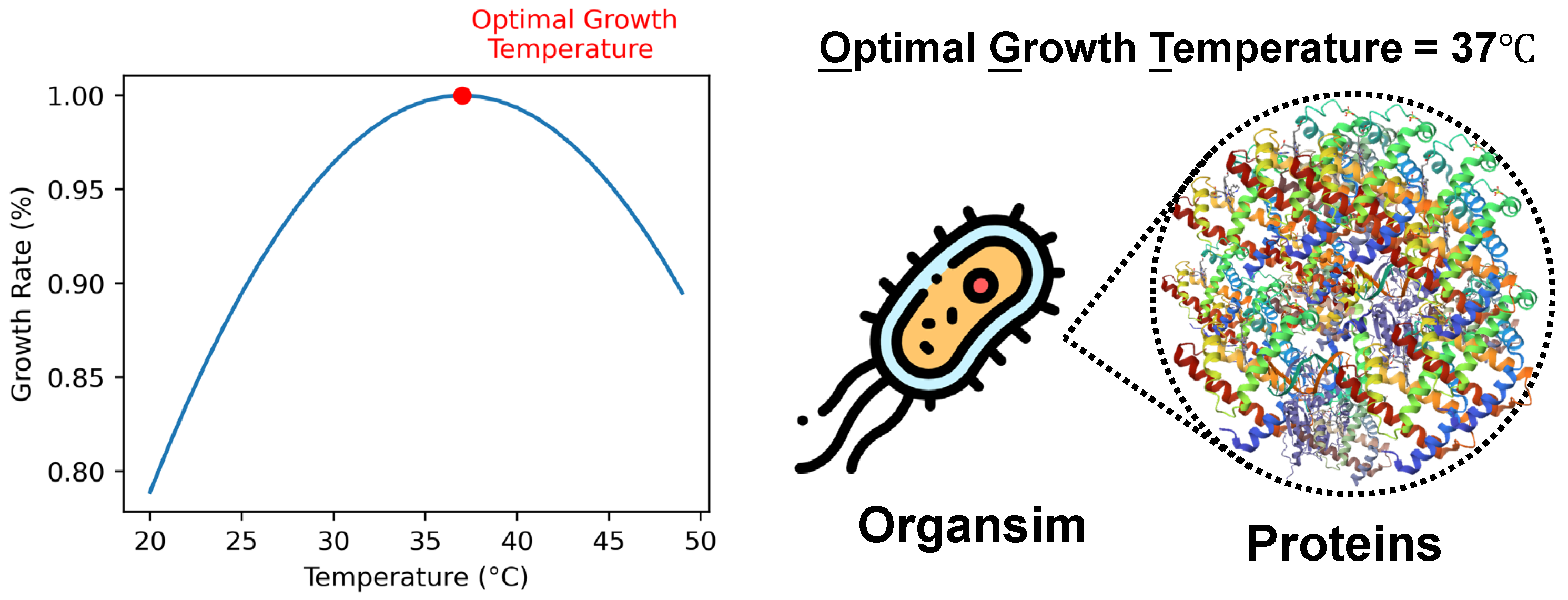
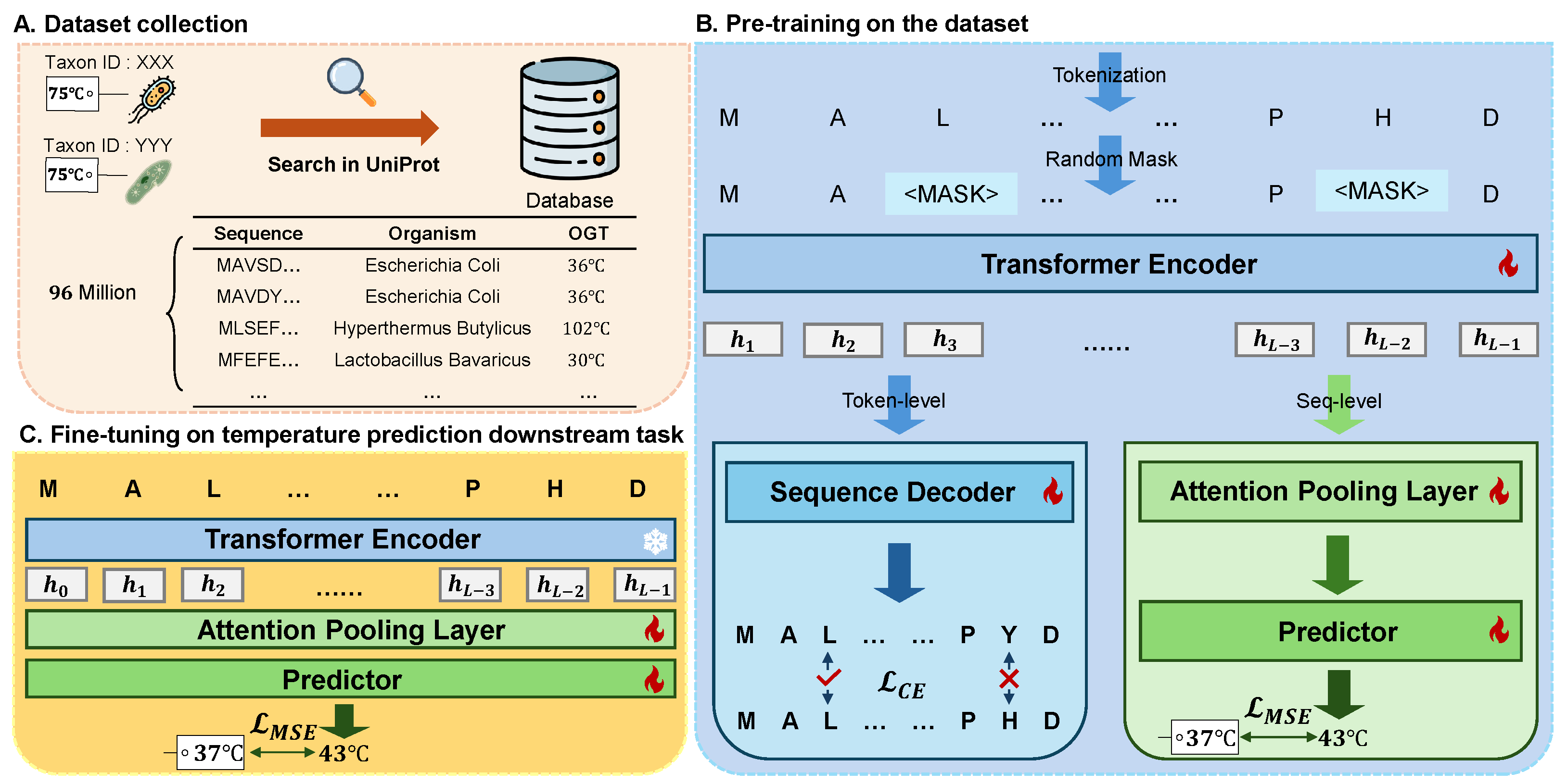
We first collected a dataset comprising 21,498 microorganisms and their corresponding optimal growth temperatures (OGTs) from the literature [41]. We queried the UniRef100 [42] database (release 2023_05) using the TaxID field in the UniRef FASTA description to retrieve all protein sequences associated with each organism (the mapping script is available at https://github.com/ginnm/ThermoFormer/blob/main/build_ogt_dataset.py (accessed on 19 March 2026)). Each protein was then annotated with the OGT of its host organism. When multiple OGT values were reported for the same taxon ID, we adopted the mean value. In our dataset, 1080 out of 18,534 organisms (∼5.8%) had conflicting OGT annotations from multiple sources; the mean absolute difference among conflicting entries was 0.98 °C. Because the UniRef100 database clusters sequences at 100% sequence identity, each unique protein maps to exactly one representative taxon ID, so OGT conflicts arise only at the organism level. We applied the following filtering pipeline: sequences containing non-standard amino acid residues (B, J, O, U, X, Z) were removed (490,316 sequences); sequences longer than 2048 residues or shorter than 32 residues were also excluded (410,699 and 39,412 sequences, respectively). Exact-duplicate sequences are not present in UniRef100 by construction. After filtering, the final OGT dataset contains 96,017,137 sequences from 14,612 organisms.

We split the pre-training dataset into a validation set, a mix-species test set, and a cross-species test set. The split is performed at the species level using NCBI Taxonomy IDs. The validation set and the cross-species test set each contain 100 organism species, identified by unique NCBI Taxonomy IDs, that are entirely absent from the training set. We verified that no organism appears under multiple taxon IDs by cross-referencing the NCBI Taxonomy database. The complete lists of taxon IDs for the 100 validation-set and 100 cross-test organisms are published in our GitHub repository (https://github.com/ginnm/ThermoFormer (accessed on 19 March 2026)) for full reproducibility. The mixed-species test set contains 500,000 sequences randomly drawn from the training organisms. A data leakage analysis using MMseqs2, including sequence identity statistics between downstream test sets (TM-Cell, TM-Atlas, OCT) and the pre-training corpus, is provided in Supplementary Note S1. Genus-level generalization analysis and a discussion of OGT label noise are provided in Supplementary Notes S4 and S5, respectively.

The statistical information of our dataset and splits is shown in

Table 11. Statistics of the pre-training dataset.

Splitting	# Organsims	# Sequences	OGT				Seqeunce Lengths
			Min. (°C)	Max. (°C)	Avg. (°C)	Std. (°C)	Min.	Max.	Avg.	Std.
Training	14,412	95,038,959	3	103	31.25	6.14	32	2048	357	245
Validation	100	502,979	15	70	30.27	5.6	32	2048	354	235
Cross-Test	100	475,199	10	57	29.31	5.2	32	2048	360	257
Mix-Test	9363	500,000	3	103	31.24	6.13	32	2048	257	245
Total	14,612	96,017,137	3	103	31.23	6.15	32	2048	357	245

.

5.2. Model Architecture and Pre-Training

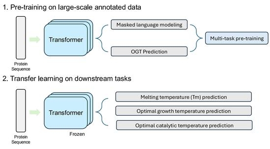
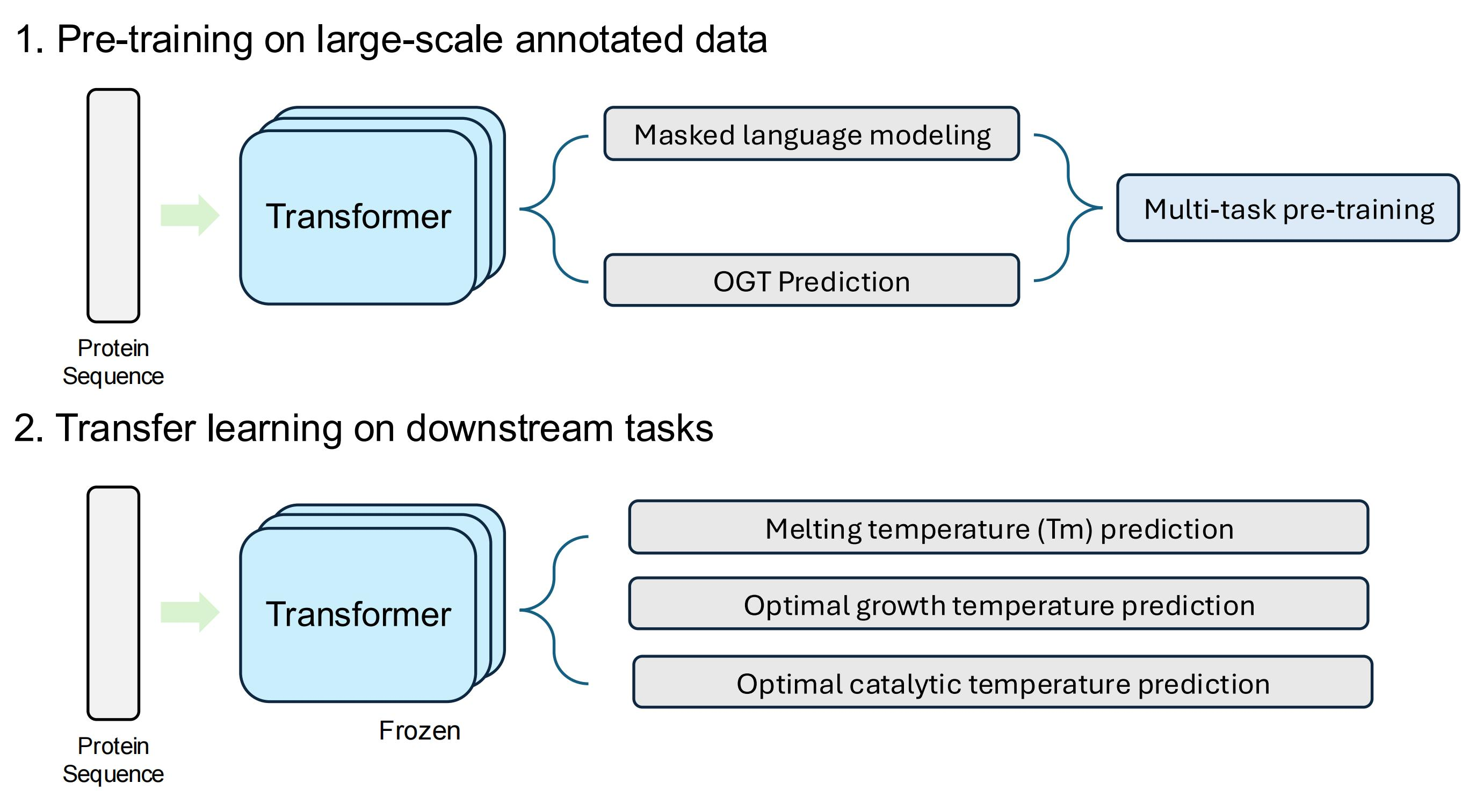
ThermoFormer is a pre-trained Transformer model. It contains four components: a transformer-based encoder for extracting residue-level representations, an attention-based pooling layer for aggregating the residue-level representation into a sequence-level representation, a sequence decoder for MLM pre-training, and a predictor for OGT prediction.

Design Rationale. While Transformer-based architectures and masked language modeling are established techniques in protein language modeling [21,23,28], ThermoFormer’s key novelty lies in the integration of large-scale supervised OGT pre-training with unsupervised MLM at an unprecedented scale of 96 million sequences. We adopt an MLM-based encoder rather than causal language modeling (CLM) because MLM produces bidirectional representations that capture the global context of protein sequences, which is essential for predicting properties determined by the entire sequence [20,30]. The combination of supervised and unsupervised objectives is designed to incorporate temperature-aware information into the learned representations while preserving the MLM objective’s sequence-understanding capability. We use an attention-based pooling mechanism rather than simpler alternatives (e.g., mean pooling or [CLS] token) because temperature-related information may be unevenly distributed across residue positions, and the attention mechanism can learn to selectively weight the most informative positions. These design choices are validated by our ablation studies in Section 4.4.

These components are detailed below:

Transformer-based encoder. The Transformer-based encoder [19] encodes the protein sequences into a sequence of contextual hidden states. Let $\mathit{s}=({\mathit{r}}_1,{\mathit{r}}_2,\dots ,{\mathit{r}}_L)\in {\mathcal{R}}^{L\times V}$ denote a protein sequence, where ${\mathit{r}}_i\in {\mathcal{R}}^V$ is the one-hot encoding of the $i_{th}$ residue, L is the length of the protein and V is the residue vocab size. The encoder first maps each residue into a dense vector through a learnable token embedding matrix:

$${\mathit{x}}_i=\mathit{E}{\mathit{r}}_i,i=1,\dots ,L$$

(1)

where $\mathit{E}\in {\mathcal{R}}^{d\times V}$ is the token embedding matrix and d is the hidden dimension. Instead of additive positional embeddings, we adopt Rotary Position Embedding (RoPE) [43], which encodes positional information by rotating the query and key vectors in the self-attention mechanism. Specifically, for position i, the rotation matrix ${\mathit{R}}_i\in {\mathcal{R}}^{d_k\times d_k}$ is defined as follows:

$${\mathit{R}}_i=\left(\begin{array}{cccc}cosi{\omega }_1& -sini{\omega }_1& & \\ sini{\omega }_1& cosi{\omega }_1& & \\ & & \ddots & \\ & & cosi{\omega }_{d_k/2}& -sini{\omega }_{d_k/2}\\ & & sini{\omega }_{d_k/2}& cosi{\omega }_{d_k/2}\end{array}\right)$$

(2)

where ${\omega }_j$ = ${\mathrm{10,000}}^{-2j/d_k}$ for $j=1,\dots ,d_k/2$. The rotation is applied to the query and key vectors before computing the attention scores, enabling the attention to be a function of relative positions between residues rather than absolute positions. This property is particularly beneficial for protein sequences, as the functional relevance of residue interactions often depends on their relative spacing in the sequence rather than their absolute positions.

The embedded sequence $({\mathit{x}}_1,{\mathit{x}}_2,\dots ,{\mathit{x}}_L)$ is then processed through N stacked Transformer layers. Each Transformer layer l consists of a multi-head self-attention (MHSA) sub-layer followed by a position-wise feed-forward network (FFN) sub-layer, each equipped with residual connections and layer normalization [44]:

$$\begin{array}{cc}\hfill {\mathit{z}}_i^{\left(l\right)}& =F_{LN}\left({\mathit{h}}_i^{(l-1)}+\mathrm{MHSA}{\left({\mathit{h}}_1^{(l-1)},\dots ,{\mathit{h}}_L^{(l-1)}\right)}_i\right)\hfill \end{array}$$

(3)

$$\begin{array}{cc}\hfill {\mathit{h}}_i^{\left(l\right)}& =F_{LN}\left({\mathit{z}}_i^{\left(l\right)}+\mathrm{FFN}\left({\mathit{z}}_i^{\left(l\right)}\right)\right)\hfill \end{array}$$

(4)

where ${\mathit{h}}_i^{\left(0\right)}={\mathit{x}}_i$ and $F_{LN}$ denotes the layer normalization function.

In the multi-head self-attention sub-layer, the input is projected into K parallel attention heads. For the k-th head, the query, key, and value vectors are computed as follows:

$${\mathit{q}}_i^{\left(k\right)}={\mathit{W}}_Q^{\left(k\right)}{\mathit{h}}_i,{\mathit{k}}_i^{\left(k\right)}={\mathit{W}}_K^{\left(k\right)}{\mathit{h}}_i,{\mathit{v}}_i^{\left(k\right)}={\mathit{W}}_V^{\left(k\right)}{\mathit{h}}_i$$

(5)

where ${\mathit{W}}_Q^{\left(k\right)},{\mathit{W}}_K^{\left(k\right)},{\mathit{W}}_V^{\left(k\right)}\in {\mathcal{R}}^{d_k\times d}$ are the projection matrices and $d_k=d/K$ is the dimension per head. The RoPE rotation is then applied to the query and key vectors before computing the attention scores:

$${\tilde{\mathit{q}}}_i^{\left(k\right)}={\mathit{R}}_i{\mathit{q}}_i^{\left(k\right)},{\tilde{\mathit{k}}}_i^{\left(k\right)}={\mathit{R}}_i{\mathit{k}}_i^{\left(k\right)}$$

(6)

This ensures that the dot product ${\tilde{\mathit{q}}}_i^{\left(k\right)\top }{\tilde{\mathit{k}}}_j^{\left(k\right)}$ depends only on the relative position $(i-j)$, since ${\mathit{R}}_i^{\top }{\mathit{R}}_j={\mathit{R}}_{j-i}$. The scaled dot-product attention is then computed as follows:

$${\mathrm{Attn}}^{\left(k\right)}=\mathrm{softmax}\left({\displaystyle \frac{{\tilde{\mathit{Q}}}^{\left(k\right)}{\tilde{\mathit{K}}}^{\left(k\right)\top }}{\sqrt{d_k}}}\right){\mathit{V}}^{\left(k\right)}$$

(7)

where ${\tilde{\mathit{Q}}}^{\left(k\right)}$ and ${\tilde{\mathit{K}}}^{\left(k\right)}$ are matrices formed by stacking the rotated query and key vectors, respectively. The outputs from all K heads are concatenated and linearly projected:

$$\mathrm{MHSA}\left(\mathit{H}\right)=\mathrm{Concat}\left({\mathrm{Attn}}^{\left(1\right)},\dots ,{\mathrm{Attn}}^{\left(K\right)}\right){\mathit{W}}_O$$

(8)

where ${\mathit{W}}_O\in {\mathcal{R}}^{d\times d}$ is the output projection matrix.

The position-wise feed-forward network consists of two linear transformations with a GELU [45] activation function:

$$\mathrm{FFN}\left(\mathit{z}\right)={\mathit{W}}_{f2}\sigma \left({\mathit{W}}_{f1}\mathit{z}+{\mathit{b}}_{f1}\right)+{\mathit{b}}_{f2}$$

(9)

where ${\mathit{W}}_{f1}\in {\mathcal{R}}^{d_{ff}\times d}$, ${\mathit{W}}_{f2}\in {\mathcal{R}}^{d\times d_{ff}}$ are weight matrices, ${\mathit{b}}_{f1}\in {\mathcal{R}}^{d_{ff}}$, ${\mathit{b}}_{f2}\in {\mathcal{R}}^d$ are bias terms, $\sigma$ is the GELU activation function, and $d_{ff}=4d$ is the intermediate dimension.

After N Transformer layers, the final contextual representations are:

$$({\mathit{h}}_1,{\mathit{h}}_2,\dots ,{\mathit{h}}_L)=({\mathit{h}}_1^{\left(N\right)},{\mathit{h}}_2^{\left(N\right)},\dots ,{\mathit{h}}_L^{\left(N\right)})$$

(10)

where ${\mathit{h}}_i\in {\mathcal{R}}^d$ is the contextual embedding of the i-th residue, capturing both local amino acid identity and global sequence context. In our implementation, the encoder comprises $N=33$ layers with $K=20$ attention heads and a hidden dimension of $d=1280$, resulting in approximately 650 million parameters. We adopt the flash attention mechanism [40] to improve computational efficiency during both pre-training and inference.

Sequence Decoder. The sequence decoder learns to recover the masked token from the hidden states. It contains two position-wise dense layers with GELU activation unit and a layer normalization layer [44]:

$$\begin{array}{c}\hfill \forall i\in 1,\dots ,L,{\mathit{y}}_i={\mathit{W}}_2^T{F}_{LN}\left(\sigma \left({\mathit{W}}_1^T{\mathit{h}}_i\right)\right)+\mathit{b}\end{array}$$

(11)

where ${\mathit{W}}_1\in {\mathcal{R}}^{d\times d}$, ${\mathit{W}}_2\in {\mathcal{R}}^{d\times V}$ and $\mathit{b}\in {\mathcal{R}}^V$ are learnable parameters, $F_{LN}$ is the layer normalization function and $\sigma$ is the GELU [45] activation function. ${\mathit{y}}_i\in {\mathcal{R}}^V$ is the probability distribution of the predicted $i_{th}$ residue. And we utilize cross-entropy as the loss function:

$$L_{CE}=-\mathbb{E}\left[log{\mathit{y}}_i\left[{\mathit{y}}_i^{*}\right]\right]$$

(12)

where ${\mathit{y}}_i^{*}$ represents the true residue for the i-th token in the sequence, and ${\mathit{y}}_i\left[{\mathit{y}}_i^{*}\right]$ denotes the predicted probability for the correct residue.

Attention-based Pooling Layer. The attention-based pooling layer learns to aggregate the hidden states $({\mathit{h}}_1,{\mathit{h}}_2,\dots ,{\mathit{h}}_L)$ into a global hidden state for further adaptation on a sequence-level task. The weights of hidden states $({\mathit{h}}_1,{\mathit{h}}_2,\dots ,{\mathit{h}}_L)$ are computed by a projection-soft-max layer that produces a weighted vector $\mathit{c}$:

$$\begin{array}{cc}\hfill ({\widehat{\mathit{h}}}_1,{\widehat{\mathit{h}}}_2,\dots ,{\widehat{\mathit{h}}}_N)& =F_{LN}({\mathit{h}}_1,{\mathit{h}}_2,\dots ,{\mathit{h}}_N)\hfill \\ \hfill s_i& ={\displaystyle \frac{e^{{\mathit{W}}_a{\widehat{\mathit{h}}}_i+{\mathit{b}}_a}}{{\sum }_{n=1}^L{e}^{{\mathit{W}}_a{\widehat{\mathit{h}}}_n+{\mathit{b}}_a}}},\forall i\in 1,\dots ,L\hfill \\ \hfill \mathit{c}& =\sum _{n=1}^L{s}_i·{\mathit{h}}_i\hfill \end{array}$$

(13)

where $s_i$ is the attention weight of the $i_{t}h$ residue and ${\mathit{W}}_a$ and ${\mathit{b}}_a$ are the learnable parameters of the attention pooling layer. Then, a multi-layer perceptron with two dense layers and GELU activation is employed to transform the weighted vector $\mathit{c}$. The first dense layer maps $\mathit{c}$ to the same dimension as the Feed-Forward Network (FFN) layer of the Transformer encoder, which in our implementation is four times the size of the hidden layer. The second dense layer maps the output of the first layer back to the original dimension. Between the first and second dense layers, a GELU activation function is applied. Additionally, there is a residual connection between the output of the second dense layer and the output of the attention layer:

$$\mathit{r}=\mathit{c}+{\mathit{W}}_4\left(\sigma ({\mathit{W}}_3\mathit{c}+{\mathit{b}}_3)\right)+{\mathit{b}}_4,$$

(14)

where ${\mathit{W}}_3,{\mathit{W}}_4,{\mathit{b}}_3,$ and ${\mathit{b}}_4$ are learnable parameters layers, $\sigma$ is the GELU activation function. The output hidden state $\mathit{r}$ is the representation of the whole sequence.

Predictor. The predictor learns to predict a temperature value $T\in \mathcal{R}$ from the sequence representation $\mathit{r}$. It has two dense layers and a $Tanh$ activation function:

$$\widehat{T}=\mathit{r}+{\mathit{W}}_6\left({\sigma }_t({\mathit{W}}_5\mathit{r}+{\mathit{b}}_5)\right)+{\mathit{b}}_6$$

(15)

where ${\mathit{W}}_5,{\mathit{W}}_6,{\mathit{b}}_5,$ and ${\mathit{b}}_6$ are learnable parameters, ${\sigma }_t$ is the Thanh activation function, and $\widehat{T}$ is the predicted temperature. We utilize the mean square error (MSE) criterion as the loss function:

$$L_{MSE}=\mathbb{E}\left[{(\widehat{T}-T)}^2\right]$$

(16)

where $\mathbb{E}[·]$ denotes the expectation, $\widehat{T}$ is the predicted temperature, and T is the ground truth temperature.

Joint Loss Function. The pre-training loss function is the sum of $L_{CE}$ and $L_{MSE}$. Since we have observed that $L_{MSE}$ has a significantly different magnitude compared to $L_{CE}$, with values ranging from 0 to 1000 initially and stabilizing at 0 to 100 later. We multiplied $L_{MSE}$ by 0.01 to maintain numerical stability. The final joint loss function is:

$$L=\beta L_{MSE}+L_{CE}$$

(17)

5.3. Supervised Fine-Tuning Paradigm

As shown in Figure 3C, we can further fine-tune ThermoFormer on other temperature prediction tasks. For the temperature prediction task, we removed the sequence decoder during the fine-tuning stage, while retaining the remaining components. The parameters were inherited from those of the pre-trained model. The Transformer encoder was kept frozen, and we fine-tuned only the parameters of the attention-based pooling layer and the predictor to reduce training cost. The subsequent experiments demonstrate that this transfer-learning approach effectively improves the Transformer model’s convergence speed and accuracy during training.

6. Conclusions

In conclusion, ThermoFormer is a protein language model that efficiently learns temperature-aware representations by combining supervised OGT prediction with unsupervised masked language modeling on a dataset of over 96 million protein sequences. Through comprehensive experiments, including ablation studies on model size, loss balancing, pooling strategies, and pre-training objectives, we have systematically validated each design choice. ThermoFormer achieves state-of-the-art performance on OGT, TM, and OCT prediction tasks, as well as on thermophilic protein classification. We believe ThermoFormer can serve as a foundation model for efficiently transferring to various downstream tasks related to protein thermal properties, and the proposed pre-training paradigm offers a template for incorporating other environmental annotations into protein language models.