Abstract
A model of production funds acquisition, which includes two differential links of the zero order and two series-connected inertial links, is considered in a one-sector economy. Zero-order differential links correspond to the equations of the Ramsey model. These equations contain scalar bounded control, which determines the distribution of the available funds into two parts: investment and consumption. Two series-connected inertial links describe the dynamics of the changes in the volume of the actual production at the current production capacity. For the considered control system, the problem is posed to maximize the average consumption value over a given time interval. The properties of optimal control are analytically established using the Pontryagin maximum principle. The cases are highlighted when such control is a bang-bang, as well as the cases when, along with bang-bang (non-singular) portions, control can contain a singular arc. At the same time, concatenation of singular and non-singular portions is carried out using chattering. A bang-bang suboptimal control is presented, which is close to the optimal one according to the given quality criterion. A positional terminal control is proposed for the first approximation when a suboptimal control with a given deviation of the objective function from the optimal value is numerically found. The obtained results are confirmed by the corresponding numerical calculations.
1. Introduction
The elements of the zero order (multiplier, accelerator), first order (inertial links), and second order are often found in nonlinear models of economic dynamics [1]. The link of the second order can be represented by an oscillatory link or by two connected inertial links. An example of a mathematical model containing inertial links is a model that takes into account the delay in the introduction of funds in the problem of optimizing the accumulation rate for the Ramsey model [1].
In this article, the following model for the development of the introduced production capacities is considered
where is the volume of the entire production capacity at time t, represents the volume of actual production at production capacity (). Here, is the total consumption at time t, defines a control function, represents a production function [1], and , are positive parameters.
The first and third equations of system (6) refer to dynamic links. The first equation describes the dynamics of changes in the volume of the introduced production capacities, the third equation sets the dynamics of the consumption process. The second equation refers to the oscillatory link characterizing the dynamics of the development of the introduced production capacities [1].
The equations of the dynamical change in the introduced production capacities of the Ramsey model [1,2,3,4,5] are used as dynamic links. They contain a scalar bounded control , which defines the distribution of the available funds into two parts: investment and consumption.
The optimization problem consists of finding a control that transfers system (6) from a given initial position to a position at the maximum value of , which is an indicator of the average consumption value over a given time interval .
The solution of the optimal control problem for this version of the model provides important information about the extreme value of the objective function and the type of optimal control. This control can contain singular controls of the third order, the direct implementation of which in economic practice can be complicated by the presence of chattering regimes. Consideration of suboptimal controls overcomes this difficulty. However, the question arises of finding a suboptimal control for which the deviation in the objective function satisfies the given constraint. The search for such a control can be realized numerically and the initial approximation is chosen in the form of a positional terminal control. The obtained properties of the optimal, suboptimal, and terminal controls for the considered model are confirmed by corresponding numerical calculations.
2. Statement of the Dynamic Model and Maximization Problem
Let us transform system (6) by introducing new phase variables: is the volume of the actual production at production capacity , and is the volume of the actual production at production capacity . In addition, we assume that the increase in production is proportional to the under-utilized capacity. All this makes it possible to rewrite the second-order differential equation in system (6) in the form of two first-order differential equations. As a result, on a given time interval , we have the following system of differential equations:
with the initial and final phase constraints:
where , , , are the phase variables; , , are the corresponding initial conditions; , , , T, are the positive parameters.
Here, is a neoclassical production function [3,5], that is, a linearly homogeneous production function satisfying the conditions:
Next, is a control function that obeys the following constraints:
We consider that the set of all admissible controls is formed by all possible of Lebesgue measurable functions , which for almost all satisfy inequalities (4).
Model (2) of the dynamics of the economic quantities includes four phase variables, the first of which is the volume of the entire production capacity, the fourth is specific consumption, and the third is the amount of funds available for use at the current time t [1,5,6].
Now, let us consider for system (2) on the set of admissible controls the following maximization problem:
The objective function in (5) means maximization of the average amount of funds allocated for consumption over a given time interval .
3. Properties of Solution of System (2)
Note that the system of Equation (2) satisfies the conditions of the Cauchy–Peano existence theorem [7], and hence, the solution of this system corresponding to the control exists (at least locally) in the neighborhood of initial point .
Now, the lower bounds for the components of the solution to system (2) are established using the following lemma.
Lemma 1.
Let be an arbitrary admissible control and
be the corresponding solution of system (2) defined for . Then the following relationships are true:
Proof.
According to the first equation of system (2), due to the conditions for the function and the restrictions on the control , we have the following relationship:
Integrating it, we obtain the required inequality: .
Due to this inequality, we have similar expression for the second equation of this system:
Hence, we find that .
Similarly, from the last inequality and the third equation of the system, we obtain:
Then it implies that .
Finally, due to the nonclassical conditions on the function and the restrictions on the control , we easily conclude that . □
Now, let us introduce the following positive values:
The next lemma shows that an arbitrary solution of system (2) exists on the entire time interval .
Lemma 2.
The solution
of system (2) corresponding to the control is defined for all .
Proof.
Let us show that for any admissible control , the corresponding solution of system (2) cannot go into infinity over a finite time interval. We assume that this solution is defined on a certain interval . It follows from neoclassical conditions that the function is monotonically decreasing from to 0. Actually, the L’Hôpital’s rule for calculating limits implies that
Now, let us verify directly the monotone decrease of the function . Since
then it suffices to establish the validity of the inequality for all . For this, we use the Newton–Leibniz formula . Function is decreasing (see the inequality in the neoclassical conditions), then we obtain the inequality for all . In such case,
Thus, the monotonic decrease of the function from to 0 is established.
Due to the proven property of function , we have the inequality:
and
Thus, for all the following inequality holds:
where is a positive constant.
Since
then there is a positive constant such that for all , and , the following estimate is valid:
Here, is the right-hand side of the system (2), and , are the corresponding scalar products of the vectors z, and vector z by itself. Therefore, according to the theorem on the continuation of solutions for differential equations [7] the solution for system (2) exists on the entire time interval . □
The last lemma justifies the uniqueness of the solution to the system (2).
Lemma 3.
The solution to system (2) is unique.
Proof.
Let us introduce the set . Then, when the initial conditions , the first three components of the solution to system (2) satisfy the estimates from Lemma 1, that is, for all . Due to the neoclassical conditions on the function , the functions , are defined and continuous for all . Thus, for the first three components of the right-hand side of system (2) the conditions of the uniqueness theorem [7] are satisfied. The right-hand side of the fourth equation of the system also satisfies the conditions of this uniqueness theorem, and therefore the solution to system (2) is unique. □
Lemmas 1–3 imply that for a neoclassical function and for any control , a solution to system (2) exists, is unique and is determined for all .
Below we give a solution to the Problem (2) and (5) which was found on the basis of the Pontryagin maximum principle [8,9] in the class of Lebesgue measurable functions satisfying inequalities (4) for almost all .
4. Pontryagin Maximum Principle
For the Problem (2) and (5), the Hamiltonian and Lagrangian of the phase constraints (3) have the form:
Here, , are adjoint variables, and , are Lagrange multipliers (see [9]).
The extremal control is defined by the relationship:
where is the switching function.
The adjoint system is given by the following system of differential equations:
which satisfy the boundary conditions:
We note that relationships (8) and (9) are written in terms of the corresponding partial derivatives of the Hamiltonian and the Lagrangian defined in (6).
The equation for in system (8) and the corresponding transversality conditions in (9) imply that . Moreover, an abnormal case occurs when , and a normal case corresponds to equality . In the abnormal case, we have . It is proven by contradiction that then, in accordance with the maximum principle [8,9], the switching function cannot take a zero value on a set of nonzero measure, which leads to a correction of the relationship (7). As a result, Formula (7) of the extremal control takes the form:
Let us consider further the normal case of the optimal control problem (2) and (5), when . In this case, we have .
Singular Regime
System (2) is such that, on the one hand, it is linear in control , and on the other hand, it clearly depends on time t due to the presence of the factor (it is non-autonomous). In addition, the problem under study (5) is a nonstandard, because it is a problem of finding the maximum, not for the traditional minimum. However, all these differences do not prevent us from applying the well-known theory of singular arcs [10,11]. This is due to the fact that:
- (i)
- performing a standard change of variables , , where is a new auxiliary variable, leads, on the one hand, to an increase by one in the order of the original system (2), and, on the other hand, makes such a system autonomous (see [8]);
- (ii)
- introducing a new objective function leads the considered problem (5) to the problem on minimum:
Thus, the original maximization problem (5) is easily transformed to the one for which the indicated theory is applicable. Therefore, further we will not explicitly follow the steps described above, but will imply them.
A singular regime takes place if for the switching function the equality holds identically for all . This regime is of order 3 (see [10,11]) and is characterized by the following relationships:
which imply that the five consecutive derivatives of the switching function vanish on the segment and only the sixth derivative has a nonzero term depending on the control .
Let us denote by the solution of the equation . Due to the concavity of the function , we have: , if . Thus, the chain of the inequalities
implies , which means that the control of a singular regime is admissible. For the control , the necessary optimality conditions for the singular control are satisfied (the Copp–Moyer conditions) [12]. Due to the neoclassical conditions and , we obtain the relationship:
Thus, singular regime can be part of an extremal control. Moreover, the singular set consists of phase and conjugate variables satisfying equalities (10). Since the singular control has order 3 and the strengthened Copp–Moyer condition (11) is satisfied for the corresponding singular portion, the concatenation of non-singular and singular portions is carried out by chattering. This means that there is an infinite number of switchings between the values 0 and 1, accumulating to the point of concatenation of such portions [11,12].
Lemma 4.
In problems (2) and (5), the optimal control has the form (7). It may have a singular regime of order 3, its explicit form is given by the corresponding formula in (10). The concatenation of non-singular and singular portions is performed using chattering.
Based on the obtained characteristics of the extremal control, we numerically construct a control containing chattering, and then, based on its structure, we construct an approximation in the form of a suboptimal control. For this control, the boundary conditions for the phase trajectory are satisfied, it contains a finite number of switchings between the boundary values 0 and 1, as well as intermediate constant values. Finally, the corresponding value of the objective function differs from its optimal value by some acceptable value.
5. Numerical Results
Here, for the problem (2) and (5), we present the results of numerical calculations using BOCOP [13] for the following values of its parameters:
For these parameter values, it is easy to calculate that
In Figure 1, the graphs , , , of the corresponding optimal solution are given for the following boundary conditions:
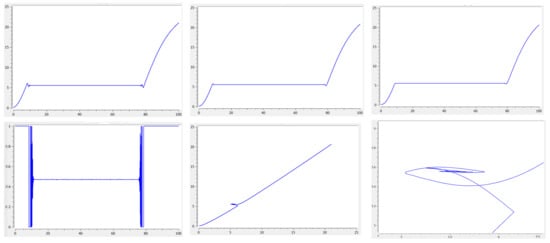
Figure 1.
Upper row: graphs of the optimal solutions , and ; lower row: the graph of the optimal control , the phase portrait , and the phase portrait in the neighborhood of the singular arc.
The optimal value of the objective function is .
Figure 1 shows the behavior of the optimal phase variables , , , and optimal control as functions of time, as well as the qualitative features of the behavior of the trajectory as a whole and when it is found on a singular set.
6. Suboptimal Control
The value of the objective function, which is close to the optimal value, can be achieved using a simpler control structure in the form:
where , , , , are variable parameters.
Let us consider the following extremal problem:
subject to the following restrictions:
Due to numerical calculations in BOCOP [13], the solution to the extremal problem (13) with parametrically specified control (12) has the form:
Figure 2 shows the graphs of approximate suboptimal control defined by (12) and of the corresponding solution for the same boundary conditions, as functions of time. The value of the objective function for such control is .
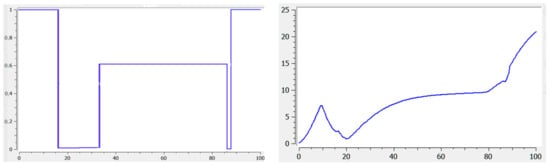
Figure 2.
Graph of the approximating control (left) and graph of the corresponding solution (right).
7. Position Controller for the Terminal Control Problem
The numerical solution of a suboptimal control problem (a control that does not contain chattering and guarantees the value of the objective function close to optimal), for example, using the method of local variations [9], requires a control of the first approximation. As such an approximation, one can use a positional controller (i.e., depending on the phase variables) for the terminal control problem for system (2), found by the method of analytical construction of aggregated controllers described in [14]. We note that the terminal control problem is the problem of transferring the phase state of the considered system from a given initial position to the required final position at some time interval.
To construct it, we introduce an additional phase variable and transform the system (2) to a form that does not contain constraints (4) on the control function:
where T is the non-fixed moment of the end of the process, and , b are positive constants.
Let us choose the value
as the first macro-variable. Here, is the intermediate control.
Then we synthesize control using a functional equation:
Then, substituting from (15) into Formula (16), we obtain an equation containing z:
From (17), the control z can be found as
Control (18) transfers the phase vector to the neighborhood of the manifold (15), the motion along which is described by the differential equations:
We will find the intermediate control from the equation
by introducing the second macro-variable
Using and Equation (19), we find the control
that transfers the phase vector to the manifold . The movement along it is described by the equation:
The solution to such an equation has the following property:
Substituting from (20) into the Formula (18), we find the desired control law
The behavior of the phase variable under control (23), starting from a certain finite time moment , is determined by the Equation (21) and, thus, we obtain the limiting relationship (22).
Moreover, the phase variable satisfies the equation
Taking into account the limiting relationship (22) of the phase variable , starting from a certain time moment , , , the variable tends to . The choice of parameters , b, , affects the values of the time moments and .
Lemma 5.
For given positive parameters μ, , , , , , δ, τ, there exist parameters , , T depending on ϵ, b, , for which the control (23) solves the terminal control problem to system (14).
The use of control (23) as the first approximation in the numerical determination of control by the method of local variations made it possible to obtain the final continuous control , for which the deviation of the objective function from the optimal value is 2%. From the last equation of system (14), it is possible to obtain the value of under control (23). Graphs of the solutions and to system (14) and trajectory under control (23) for system parameters from Section 5 are shown in Figure 3.
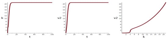
Figure 3.
Graphs of solutions and to system (14) and trajectory under control (23).
8. Conclusions
In this article, at a given time interval, the Ramsey model was used to describe the change in fixed assets of a one-sector economy. It included a bounded control function that divided the available funds into investment and consumption. In addition, differential equations have been added to this model to reflect the dynamics of the development of the introduced production capacities. The optimal control problem was posed for such a modified Ramsey model, which consisted in maximizing the average consumption over a given period of time. For an analytical description of the properties of the corresponding optimal control, the Pontryagin maximum principle was applied. Situations were found where this control was a bang-bang function, as well as where it was capable of containing a singular regime concatenating to non-singular bang-bang portions using chattering. It is clear that such a phenomenon as chattering cannot be implemented in real economic processes, and therefore an approach was proposed in the article to find suboptimal control, which would be close to the optimal in terms of the considered objective function. This approach requires a good initial approximation. As such an approximation, the article proposed to use positional terminal control. The corresponding numerical calculations were carried out, which showed the effectiveness of the proposed approach.
Author Contributions
Conceptualization, N.G. and L.L.; methodology, N.G. and L.L.; software, L.L.; validation, N.G. and L.L.; formal analysis, L.L.; investigation, N.G. and L.L.; resources, N.G. and L.L.; data curation, not applicable; writing–original draft preparation, N.G. and L.L.; writing–review and editing, N.G. and L.L.; visualization, N.G. and L.L.; supervision, N.G.; project administration, not applicable; funding acquisition, not applicable. All authors have read and agreed to the published version of the manuscript.
Funding
This research received no external funding.
Conflicts of Interest
The authors declare no conflict of interest.
References
- Kolemaev, V.A. Mathematical Economics; Yuniti-Dana: Moscow, Russia, 2015. [Google Scholar]
- Grass, D.; Caulkins, J.P.; Feichtinger, G.; Tragler, G.; Behrens, D.A. Optimal Control of Nonlinear Processes. With Applications in Drugs, Corruptions, and Terror; Springer: Berlin/Heidelberg, Germany, 2008. [Google Scholar]
- Ramsey, F.P. A mathematical theory of saving. Econ. J. 1928, 38, 543–559. [Google Scholar] [CrossRef]
- Seierstad, A.; Sydsæter, K. Optimal Control Theory with Economic Applications; North-Holland: Amsterdam, The Netherlands, 1987. [Google Scholar]
- Shell, K. Applications of Pontryagin’s maximum principle to economics. In Mathematical Systems Theory and Economics 1; Springer: Berlin, Germany, 1969; pp. 241–292. [Google Scholar]
- Spear, S.E.; Young, W. Optimum savings and optimal growth: Ramsey–Mavlinvaud–Koopmans nexus. Macroecon. Dyn. 2014, 18, 215–243. [Google Scholar] [CrossRef]
- Pontryagin, L.S. Ordinary Differential Equations; Addison-Wesley Publishing Company: London, UK, 1962. [Google Scholar]
- Pontryagin, L.S.; Boltyanskii, V.G.; Gamkrelidze, R.V.; Mishchenko, E.F. Mathematical Theory of Optimal Processes; John Wiley & Sons: New York, NY, USA, 1962. [Google Scholar]
- Vasiliev, F.P. Optimization Methods; Factorial Press: Moscow, Russia, 2002. [Google Scholar]
- Afanasiev, V.N.; Kolmanovskii, V.; Nosov, V.R. Mathematical Theory of Control Systems Design; Springer: Dordrecht, The Netherlands, 1996. [Google Scholar]
- Schättler, H.; Ledzewicz, U. Optimal Control for Mathematical Models of Cancer Therapies: An Application of Geometric Methods; Springer: New York, NY, USA; Heidelberg, Germany; Dordrecht, The Netherlands; London, UK, 2015. [Google Scholar]
- Zelikin, M.I.; Borisov, V.F. Theory of Chattering Control: With Applications to Astronautics, Robotics, Economics and Engineering; Birkhäuser: Boston, MA, USA, 1994. [Google Scholar]
- Bonnans, F.; Martinon, P.; Giorgi, D.; Grélard, V.; Maindrault, S.; Tissot, O.; Liu, J. BOCOP 2.2.0—User Guide. Available online: http://bocop.org (accessed on 27 June 2019).
- Kolesnikov, A.; Veselov, G.; Kolesnikov, A.; Monti, A.; Ponci, F.; Santi, E.; Dougal, R. Synergetic synthesis of Dc-Dc boost converter controllers: Theory and experimental analysis. In Proceedings of the 17th Annual IEEE Applied Power Electronics Conference and Exposition, Dallas, TX, USA, 10–14 March 2002; pp. 409–415. [Google Scholar]
Publisher’s Note: MDPI stays neutral with regard to jurisdictional claims in published maps and institutional affiliations. |
© 2021 by the authors. Licensee MDPI, Basel, Switzerland. This article is an open access article distributed under the terms and conditions of the Creative Commons Attribution (CC BY) license (http://creativecommons.org/licenses/by/4.0/).