Highlights
What are the main findings?
- The Gulf exhibits two distinct dynamical regimes: a transient north versus a persistent, topographically trapped south.
- Long-lived eddies at the mouth of the Gulf of California are predominantly cyclonic and exhibit coherent poleward propagation consistent with advection by the Mexican Coastal Current.
What are the implications of the main findings?
- Mesoscale structures near the entrance facilitate significant meridional connectivity and transport biogeochemical properties up-basin, acting as active exchange pathways between the Pacific Ocean and the Gulf of California.
Abstract
Mesoscale eddies play a key role in oceanic transport, yet their characterization in marginal seas like the Gulf of California remains challenging due to complex coastlines and bathymetry that hinder conventional detection methods. This study addresses this gap by presenting a robust hybrid framework—integrating dynamical (Okubo–Weiss), velocity geometry (Nencioli), and closed-contour (Chelton) criteria—applied to the high-resolution () Neural Ocean Surface Topography (NeurOST) altimetry product (2010–2024). Temporal continuity is ensured through a cost-based tracking algorithm optimized to tolerate observational gaps and track quasi-stationary features. This census, representing the first systematic, high-resolution sea surface height anomaly (SSHA)-based characterization for this region, identified 344 persistent trajectories (≥14 days) and revealed a fundamental dichotomy in the Gulf’s dynamics: a transient, tidally dominated regime in the north (dominated by short-lived features) contrasting sharply with a persistent, topographically trapped regime in the south. Focusing on the long-lived population (lifetimes days), our analysis confirms that multi-year, quasi-stationary cyclonic eddies are trapped in the southern basins, while a subset of energetic tracks exhibits coherent poleward propagation consistent with advection by the Mexican Coastal Current. Cyclonic structures dominate the ten longest-lived tracks (90%) and include two events with lifetimes confirmed to exceed 500 days. We also identify a robust seasonal decoupling between SSHA and sea surface temperature anomalies (SSTA) in spring, when surface heating masks the thermal signature of cyclones. This census, which documents multi-year structures and distinguishes the two regional regimes, establishes a new baseline for quantifying mesoscale transport and serves as a transferable framework for the new generation of satellite altimetry observations (i.e., the Surface Water and Ocean Topography, SWOT, mission).
1. Introduction
Satellite altimetry has transformed the study of ocean dynamics by enabling systematic observations of mesoscale variability at the global scale [1,2]. Among these features, oceanic eddies represent one of the most energetic manifestations of mesoscale circulation, accounting for nearly 80% of the ocean’s kinetic energy [1,3]. They are defined as coherent rotational structures that can persist from weeks to months and play a fundamental role in the redistribution of heat, salt, nutrients, and biomass, with direct implications for marine productivity and regional climate [4,5].
The study of mesoscale dynamics is particularly critical in marginal and semi-enclosed basins. Unlike the open ocean, the circulation in these regions is strongly influenced by complex coastal boundaries and abrupt bottom topography, which often constrain eddy formation and evolution. The intense tidal mixing and stratification effects common in these environments, such as those driven by dissipation over sills [6], critically affect how mesoscale structures evolve and redistribute properties. The efficient transport of heat, salt, and nutrients by these features fundamentally regulates biological productivity and regional climate in these constricted seas [4].
Our study focuses on the Gulf of California (GC), a semi-enclosed, evaporation-driven sea of significant dynamical and ecological importance [7], given its high biodiversity, great primary productivity, and its role as one of Mexico’s most important fishing regions. The GC extends approximately 1100 km in a northwest–southeast direction between the Baja California Peninsula and the Mexican mainland, with a width between 150 and 200 km. Its only connection to the Pacific Ocean is through the southern mouth, which strongly influences its hydrography and circulation [7]. The bathymetry of the Gulf is complex, divided by a series of sills and the Midriff Islands (near N) into two distinct basins: a shallow, seasonally forced northern region and a deep southern region characterized by a chain of basins (Figure 1). This natural division creates different dynamical regimes [7,8].
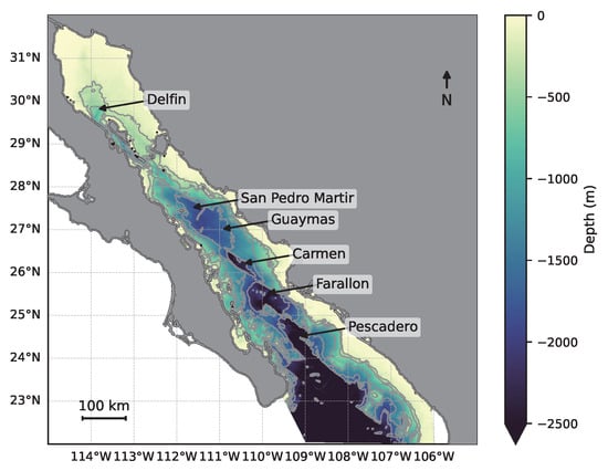
Figure 1.
Bathymetry of the Gulf of California derived from the GEBCO 2025 global grid [9]. Depth is indicated by color shading, with shallower regions in light green and deeper basins (Delfin, San Pedro Martir, Guaymas, Carmen, Farallon, and Pescadero) in dark blue. Contours (250, 500, 1000, 2000 m) highlight the steep topographic gradients that characterize the Gulf’s morphology.
In the GC, mesoscale eddies have been widely reported through in situ measurements (e.g., [10,11]), remote sensing (e.g., ocean color and Sea Surface Temperature, SST [12,13]), and modeling approaches (e.g., [14]). Early hydrographic surveys and satellite imagery revealed alternating cyclonic and anticyclonic structures along the Gulf axis, some apparently constrained by topography [12,13,15]. Subsequent studies described their hydrographic and dynamical characteristics, showing core radii of 30–40 km, maximum surface velocities of 0.4–0.5 m , and vertical penetration of several hundred meters [8,10,11]. Crucially, while most observational studies report short life spans (typically weeks) [12], other reports suggest that coherent structures, particularly near the Gulf’s mouth, can persist for up to two or three months, exceeding the few-week lifetime [13,14]. Modeling studies suggest the main driver is the interaction between poleward eastern boundary currents and coastal topography [14], while other analyses confirmed strong seasonal and interannual variability [13,16].
Despite this extensive body of work, a systematic, long-term characterization of eddies in the GC from satellite altimetry has remained elusive. This research gap stems from two fundamental challenges. First, as noted by [8], conventional global gridded altimetry products (approx. ) are too coarse to resolve the smaller mesoscale structures typical of marginal seas. Second, the complex bathymetry and convoluted coastline of the Gulf (Figure 1) present a significant challenge for standard detection algorithms [1,17], which were designed for open-ocean conditions. Applying these methods in such a topographically complex region often leads to spurious detections and fragmented tracks. Specifically, purely geometric approaches frequently misidentify coastal meanders or upwelling filaments as coherent eddies, while methods relying on flow symmetry and velocity gradients struggle with the high noise and sharp shear zones induced by bottom friction and boundaries [1,17,18]. This has, until now, hindered the development of a robust census based on Sea Surface Height Anomaly (SSHA) fields.
Here, we address this observational and methodological gap by developing and applying a complete detection and tracking framework to the recently available high-resolution () Neural Ocean Surface Topography (NeurOST) altimetry dataset [19]. Our hypothesis is that a robust hybrid method, integrating dynamical (Okubo–Weiss), velocity geometry (Nencioli), and closed-contour (Chelton) criteria, is essential to accurately characterize mesoscale eddies interacting with complex coastal and marginal sea topography. The use of NeurOST, a product generated via a neural network, is justified by its demonstrated capacity to reconstruct mesoscale and submesoscale dynamics with higher fidelity and lower noise than conventional gridded products, making it uniquely suited for marginal seas [19,20]. Thus, we propose this robust hybrid detection method, complemented by geometric and amplitude filters. This multi-criterion approach is specifically designed to suppress spurious, transient features common in complex coastal regions. This framework enables, for the first time, consistent long-term (2010–2024) quantification of the mesoscale eddy population in the GC from SSHA fields, providing a solid foundation for analyzing their statistics, regional variability, and dynamical characteristics.
2. Materials and Methods
2.1. Satellite Datasets
This study uses high-resolution satellite products to analyze mesoscale eddies in the GC. We employ Sea Level Anomalies (SSHA; equivalent to SLA), rather than absolute Sea Surface Height (SSH), as this variable isolates mesoscale variability by removing the mean sea surface and large-scale geoid contributions [1,21]. SSHA is therefore more suitable for eddy detection, as it emphasizes rotational and advective features associated with mesoscale circulation. Although Surface Water and Ocean Topography (SWOT) Level-2 products provide absolute SSH, subtracting a Mean Sea Surface (MSS) yields SSHA fields that are methodologically consistent and directly comparable across altimetry missions [22]. We also used SST fields to compute Sea Surface Temperature Anomalies (SSTA) for thermal-dynamical comparison, which provides insight into baroclinic coherence and corroborates the SSHA structures against thermal wind balance. Two main datasets were employed:
- SSHA: The Neural Optimal Sea Surface Topography (NeurOST) dataset [20], developed using deep learning from Data Unification and Altimeter Combination System (DUACS) L3 altimetry and MUR L4 SST [19], provides daily SSHA fields at spatial resolution. We used the full data record from 1 January 2010 to 16 July 2024.
- SST: The Multi-scale Ultra-high Resolution (MUR) SST dataset [23], provides daily global coverage at 1 km spatial resolution by combining infrared and microwave observations; the methodology is described in [24].
2.2. Preprocessing and Anomaly Computation
To isolate mesoscale variability, both SSHA and SSTA fields were preprocessed prior to detection. For each grid point inside the GC mask, we applied the following steps:
- Linear trend removal: A least-squares fit was used to remove the long-term linear trend from each time series.
- Seasonal cycle removal: The annual and semi-annual harmonics were fitted and subtracted, thereby eliminating the dominant seasonal signal.
- Spatial detrending: For each daily map, a best-fit linear plane in latitude and longitude was removed to suppress large-scale background slopes and emphasize mesoscale structures.
- Regridding: Daily MUR SST fields were bilinearly interpolated onto the NeurOST grid to allow pixel-wise comparison with SSHA fields.
2.3. Eddy Detection Algorithm
We detected eddies from daily SSHA and geostrophic fields using a three-stage procedure that we developed to combine dynamical and geometric constraints (Okubo–Weiss, velocity geometry, and closed-contour checks), following established approaches for mesoscale eddy identification [1,17,25,26,27]. The three approaches emphasize the core components of eddy definition: vorticity dominance (Okubo–Weiss), flow symmetry (Nencioli), and geometric coherence (Chelton). This hybrid approach was designed to improve robustness for the GC, where complex coastlines and topography can challenge single-criterion methods.
This multi-stage process sequentially refines eddy candidates. This framework builds upon the Okubo–Weiss method (dynamical filter) and two classical detection algorithms: the closed-contour method of [1] (hereafter CHE11) and the velocity geometry criterion of [17] (hereafter NEN10), which respectively emphasize geometric and dynamical coherence.
The detection process consists of the following three stages:
- Stage 1: Vorticity–strain filter (Okubo–Weiss) and speed minima. We computed the Okubo–Weiss parameter [25,26] , where and are the normal and shear components of strain, respectively, and is the vertical component of relative vorticity. Here, u and v are the horizontal velocity components (zonal and meridional), and x and y are the corresponding spatial coordinates. This parameter was computed from the detrended geostrophic velocity anomalies and normalized by , with , where is the angular velocity of the Earth and is the latitude. Candidate pixels were defined by , where is the 10th percentile of the daily distribution, thus applying a conservative but adaptive threshold. The constant threshold is a widely used empirical value, consistent with open-ocean studies [1,28], and is applied here because selecting regions where vorticity strongly dominates strain is even more critical in the turbulent, high-resolution SSHA fields of the GC. Candidates were further restricted to local minima of the geostrophic speed, defined within a pixel neighborhood and allowing a tolerance proportional to the 95th percentile of the speed. This neighborhood size was selected as the minimal area required to define a local extremum in the gridded data while avoiding excessive smoothing of small-scale features. A binary dilation was then applied to consolidate contiguous candidate pixels into solid core regions, filling small gaps within the identified cores.
- Stage 2: Velocity geometry consistency. Candidate eddy cores were refined using the flow–symmetry conditions of NEN10, implemented with an annular search radius a. A pixel was retained only if at least six out of eight radial directions satisfied the sign-change and magnitude-decrease conditions in and (the zonal and meridional geostrophic velocities, respectively), with a relaxation factor . This value was selected based on sensitivity tests as a compromise, balancing the strict coherence of NEN10 with the slightly less regular structures observed in the high-resolution SSHA fields of this complex region. This yielded a refined mask centered on rotational cores. The hyperparameters adjusted in this and the following stages are detailed in Table 1.
 Table 1. Tracking hyperparameters (i.e., user-defined algorithm settings) and values used in this study.
 - Stage 3: Closed-contour validation on SSHA with shape and scale controls. SSHA isolines were computed from masked fields to avoid artifacts over NaNs (Not-a-Number; i.e., masked land or cloud areas), and only closed, geometrically valid contours that did not intersect the domain boundaries were retained. Each candidate contour had to satisfy a circularity threshold (, where A is the contour area and P is the perimeter). This threshold was determined through sensitivity tests as an optimal balance for this topographically complex region: it is strict enough to filter spurious, non-eddy features, yet flexible enough to retain coherent eddies during deformation (e.g., when interacting with the coast). This approach reduces artificial detection gaps and track fragmentation. Nested contours were grouped into families, and the member with the largest SSHA amplitude relative to its perimeter level was selected; a minimum amplitude of m was imposed. This value was chosen to be approximately twice the nominal root-mean-square error of the altimetry product [19], ensuring that detected features are significantly above the instrument and mapping noise level. Additional scale filters required at least 8 enclosed pixels and a maximum convex–hull diameter km, consistent with the width of the Gulf. Residual coherent “seeds” (i.e., the rotational cores identified in Stage 2) from Stage 2 not intersected by any selected contour were added if their area exceeded 10 pixels, using their convex hull as a proxy boundary. Finally, nested duplicates were removed and contours with centroids separated by less than 10 km were merged into a single eddy.
Polarity was assigned from the sign of the mean relative vorticity within the selected contour (cyclonic if , anticyclonic otherwise). The eddy center was set at the SSHA extremum inside the polygon (minimum for cyclones, maximum for anticyclones), with fallback to the geometric centroid if the extremum was undefined [1,27]. Eddy diameter was computed as twice the median radial distance from the center to the contour vertices. Major and minor axes and eccentricity were derived by applying principal-component analysis (PCA) to the boundary points, providing a robust estimate of eddy geometry [29,30,31]. Mean and mean within the eddy interior were stored for tracking.
For each day t we built (i) a boolean mask of eddy interiors and (ii) a catalogue listing time, centroid (latitude , longitude ), diameter, major and minor axes, eccentricity, polarity, mean vorticity, and mean geostrophic velocities. These fields were written to a NetCDF file for subsequent trajectory reconstruction.
2.4. Eddy Tracking
We reconstructed eddy trajectories by linking daily detections into temporally coherent tracks using a cost-based nearest-neighbour association, a strategy commonly adopted in mesoscale eddy studies (e.g., [1,32,33,34]). A robust tracking algorithm is particularly important in marginal seas like the GC, where eddy deformation by complex coastlines and topography can cause intermittent detections. In contrast to global catalogues, we introduced refinements to handle these conditions, including adaptive thresholds, a gradual gap penalty, and stricter pruning criteria. The procedure operates on the set of eddy states identified each day t, where every state stores centroid , diameter D, major/minor axes, eccentricity, relative vorticity , and polarity (cyclonic/anticyclonic). The algorithm was designed to be versatile, so that its hyperparameters (summarized in Table 1) can be adjusted for different regions of study.
For each existing track, we keep an eddy’s most recent state and an estimated constant velocity of the eddy centroid, computed between consecutive states. To handle both propagating and quasi-stationary eddies, the tracker evaluates two position hypotheses for a gap of g days (): (1) an ’inertia’ hypothesis, where the position is predicted by linear advection (Equation (1)), and (2) a ’stationary’ hypothesis, using the last known centroid :
where are in degrees and are in km . Candidate associations to a detection are evaluated using the minimum great-circle (haversine) distance from the two hypotheses: , where and . This dual approach is critical for correctly tracking eddies that become temporarily trapped by topography.
To link these daily detections, we implemented a multi-parameter cost function, J. This is a standard procedure in modern tracking algorithms, as it provides a robust quantitative metric to assess the likelihood of an association based on multiple physical properties [35]. The function (Equation (2)) balances spatial separation, relative size, vorticity, and polarity consistency. This multi-parameter approach ensures that a match is not only spatially close (term ) but also dynamically similar in size () and rotation (), while heavily penalizing physically unrealistic polarity switches ().
where d is the distance computed previously. The term represents a dynamic maximum matching distance, (km), which scales with the gap duration g (in days, ) to reflect growing positional uncertainty over time. This dynamic value is crucial for a region like the GC, as a fixed 50 km limit (common in other studies) would be too large for a 1-day gap but too small for a 10-day gap. The relative changes are defined as:
We set , making polarity mismatches virtually forbidden. These weights were optimized through sensitivity analysis: the weights for diameter () and vorticity () are reduced, as these parameters can be noisy on a daily basis, especially during coastal interactions. This configuration prioritizes spatial proximity and polarity over short-term fluctuations in eddy shape or spin, making the tracker more robust. If the best candidate occurs after a data gap (), the cost is inflated by a gap penalty , which gradually increases uncertainty while still allowing short interruptions.
At each day t, for every new detection we select the existing track with the minimum cost J provided , with . This threshold was determined through sensitivity tests to allow for moderate changes in eddy properties without permitting erroneous mergers. If no track satisfies the threshold, a new track is initialized. Tracks remain eligible for reassociation during gaps up to days, after which they are closed. This maximum gap is a physically defensible limit corresponding to approximately 1.5 times the 10-day repeat cycle of the reference altimetry missions (e.g., Jason series), allowing the algorithm to bridge realistic observational gaps [36]. Although this tolerance permits temporal gaps, the strict polarity constraint (weighted by ) ensures that distinct dynamic features are not erroneously merged during track reconstruction. Typical surface speeds – m imply daily displacements of ∼25–35 km, which are well handled by our dynamic and cost function.
When a detection is appended to a track, the along-track velocity is updated using centroid differences (Equation (4)):
where and are in degrees, is the mean latitude, is in days, and the resulting velocities are in km . The constant 111 is the standard conversion factor from degrees to kilometers. The term correctly scales the zonal distance, a formulation that is standard in oceanography [1] and introduces negligible error (≪1%) for the mid-latitudes of this study.
Finally, tracks shorter than a minimum persistence threshold, daily detections, are discarded. This step filters out transient or poorly sampled structures and retains only persistent mesoscale features. The thresholds in Table 1 were selected after sensitivity tests to minimize fragmentation and false mergers while preserving lifetimes and displacements consistent with previous eddy studies. All thresholds and weights are hyperparameters, allowing this framework to be adapted for other basins. The physical justifications provided for each (e.g., based on satellite repeat cycles, based on persistence) serve as a clear basis for their re-calibration in regions with different dynamical regimes.
2.5. SSTA Comparison and Implementation
Eddies were also identified in the SSTA field using the same closed-contour algorithm. Structures overlapping in time and space with SSHA eddies were classified as coincident. Spatial and seasonal correlations between SSHA and SSTA were computed to assess structural consistency, supporting inferences about baroclinic eddy coherence under thermal wind balance [37,38].
The tracking algorithm is implemented in Python (v3.8)and operates on the daily eddy states extracted from the NetCDF catalogue of detections (eddy_detections_hybrid_GoC_ 2010_2024.nc). Each entry is converted into an EddyState object containing time, centroid, geometry, vorticity, polarity, and a velocity placeholder. The loop proceeds chronologically, evaluates candidate costs, applies thresholded greedy assignment, updates velocities, and prunes short tracks. The procedure outputs the final track catalogs (e.g., tracks_catalog_full.nc and tracks_catalog_min14d.nc). All data products generated by this workflow are publicly available (see Data Availability Statement).
3. Results
This section presents the main outcomes of the proposed hybrid eddy detector, based on its application to the GC as a regional test case. Results are organized into five parts: (i) Comparison with Classical Detection Methods, (ii) General Statistics of Detected Eddies, (iii) Seasonal Variability of Eddy Occurrence and Intensity, (iv) SSHA–SSTA Relationship, and (v) Case Study: Long-Lived and Quasi-Stationary Eddies.
3.1. Comparison of Detection Methods
To evaluate the consistency and performance of the hybrid detector, we compared it with two classical approaches widely used in mesoscale eddy detection: the closed-contour method CHE11 and the velocity geometry criterion of NEN10. Both algorithms were implemented following their original formulations, without additional tuning, and applied over the same reference days used during the hybrid detector’s development.
Figure 2 illustrates a representative day (index 3025), showing the spatial distribution of detections by each algorithm. The CHE11 method (yellow contours) detects substantially more features (24–79 per day) than the other methods, often including unclosed meanders and small-scale, fragmented structures near the coast. In contrast, NEN10 (purple lines) yields a more conservative count (10–20 eddies per day), but produces spurious detections near islands and coastlines where velocity shear is high but no coherent vortex exists. The hybrid approach (teal and magenta) produces a stable number of detections (3–7 per day), capturing only those features that exhibit both closed SSHA contours and velocity geometry consistency, which correspond to visually coherent, well-defined mesoscale eddies.
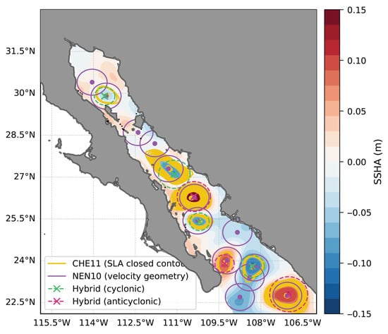
Figure 2.
Eddy detections on Day 3025 obtained by classical methods (CHE11 in yellow, NEN10 in purple) and the proposed hybrid detector (cyclonic in dashed teal, anticyclonic in dashed magenta). Background: SSHA (m) over the GC. CHE11 identifies numerous fragmented/transient features, NEN10 shows sensitivity to coastal shear, whereas the hybrid detector balances noise rejection with coherent-eddy retention.
Performance metrics for a detection period of 11 days are summarized in Table 2. We define Precision (P) as the fraction of true positives () to all detections (), Recall (R) as the fraction of TPs to all reference eddies (), and the F1-score as the harmonic mean of P and R. High Precision indicates a low rate of false alarms relative to the reference, while high Recall indicates that few reference eddies were missed. It is important to note that, since no independent observational census exists for this period, these metrics quantify the internal consistency of the hybrid method relative to the single-criterion algorithms rather than absolute detection accuracy. Using hybrid detections as reference, CHE11 achieves perfect recall (), which means that it successfully finds all eddies identified by the hybrid method. However, it has low precision (), indicating that the vast majority of its detections are considered noise or non-eddy features by the stricter hybrid criteria (31.5 excess detections per day). The NEN10 method, when strictly matching by both location and polarity, failed to match the reference eddies in this subset (, ). This discrepancy highlights that while NEN10 detects vorticity centers, it often assigns a polarity or center location that does not align with the closed SSHA contours required by the hybrid framework. Table 2 thus quantifies the selectivity of the hybrid method relative to classical single-criterion approaches.
Table 2.
Mean performance metrics of each detection method across the 11 test days. Precision (P), Recall (R), and F1-score computed using the hybrid detections as reference.
Overall, the hybrid method effectively filters inconsistent features, retaining only those vortices that satisfy both geometric and dynamical constraints, combining the strengths of CHE11 and NEN10.
3.2. General Statistics and Spatial Distribution (Gulf-Wide)
Our algorithm identified a total of 344 eddy tracks with lifetimes days over the 2010–2024 period. To focus the analysis on persistent, well-defined mesoscale structures, all subsequent statistics are calculated exclusively for long-lived eddies with lifetimes days.
This filtering yields a robust population of 208 long-lived eddies (98 cyclonic, 110 anticyclonic). Figure 3 displays the spatial distribution of eddy occurrence density for all detected tracks (≥14 days). Eddy activity is not uniform, but is concentrated in “hotspots” aligned with the central and southern deep basins (e.g., Guaymas, Carmen, and Pescadero). We note that the density map for only long-lived eddies (>30 days) is nearly identical to the total map, indicating that the Gulf’s eddy field is dominated by these persistent structures.
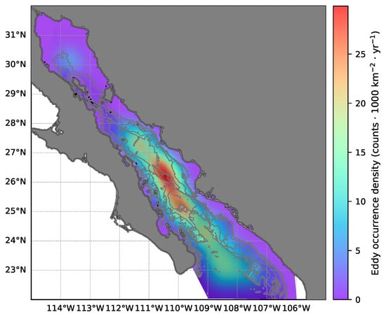
Figure 3.
Smoothed eddy occurrence density (counts · 1000 ) for all tracks (≥14 days) in the GC. Highest eddy densities (hotspots) align with the deep basins in the central and southern Gulf (e.g., Guaymas, Carmen, Farallon, Pescadero). Depth contours (250 m, 500 m, 1000 m, 2000 m) highlight the steep topographic gradients that characterize the Gulf’s morphology.
A preliminary regional analysis (split at N, near the Midriff Islands) revealed very few persistent eddies () in the shallow, topographically complex northern region. Given this statistically insignificant sample size, and to maintain the robustness of the statistical analysis, all properties are presented for the entire GC as a single region.
The spatial distribution of mesoscale intensity (Figure 4) reflects this eddy-dominated regime. SSHA RMS (Figure 4a) and mean EKE (Figure 4b) are maximum along the deep basins and toward the Gulf mouth. The RMS of normalized relative vorticity () mirrors this pattern (Figure 4c). These high-intensity patterns are the direct statistical footprint of the recurrent and persistent eddies shown in Figure 3, confirming that the central-southern channel is the primary locus of mesoscale activity.
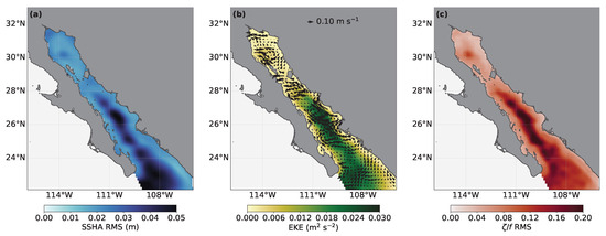
Figure 4.
Spatial variability of mesoscale intensity in the Gulf of California. (a) Root-mean-square Sea Surface Height Anomaly (SSHA RMS; m). (b) Time-mean eddy kinetic energy (EKE; ) overlaid with mean geostrophic currents (arrows). (c) Root-mean-square normalized relative vorticity (RMS ; dimensionless). High SSHA RMS and EKE concentrate along the central–southern deep basins, consistent with a bathymetrically constrained mesoscale eddy field.
The statistical properties of the long-lived eddy (>30 days) population are shown in Figure 5. Lifetimes (Figure 5a) show a median of 52.5 days for cyclones and 60.0 days for anticyclones. Diameters (Figure 5b) are also similar between polarities, with a median of 98.5 km for cyclones and 103.8 km for anticyclones. These diameters are consistent with the regional Rossby radius of deformation and the width of the southern basins [7,12]. The lifetime axis in Figure 5a is extended to capture the full range of long-lived trajectories, including the longest-lived eddies reported in Table 3.
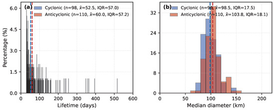
Figure 5.
Histograms of eddy properties for long-lived tracks (>30 days) in the Gulf of California. (a) Lifetimes and (b) Median diameters for cyclonic (blue, ) and anticyclonic (red, ) eddies. Dashed lines indicate the median () for each population. The interquartile range (IQR) are also shown for each set of eddies.
Table 3.
Median statistical properties for long-lived (>30 days) eddies in the Gulf of California, grouped by season. Interquartile Range (IQR) is shown in parentheses. These statistics are representative of the entire Gulf-wide persistent population.
Some statistics of the eddies, including rotational and translational speeds, is provided in Table 3. The median rotational speeds are consistently high (approx. 0.46–0.49 m ) and an order of magnitude larger than the translational speeds (approx. 0.04–0.05 m ), confirming the quasi-stationary nature of many persistent eddies.
3.3. Seasonal Variability
Figure 6 presents the Gulf-wide monthly variability for the long-lived eddy population. The normalized vorticity (, Figure 6a) exhibits a bimodal seasonal pattern, with higher intensity in winter (Jan–Mar) and a secondary peak in late summer (Aug–Oct). Translational speed (Figure 6b) is low and relatively constant year-round, with a mean of 0.05 m . Rotational speed (Figure 6c) is an order of magnitude larger than translational speed, ranging from 0.35 to 0.48 m , and follows the same seasonality as vorticity. Although Figure 6 emphasizes monthly mean behavior, the underlying distributions of eddy properties exhibit substantial dispersion, particularly during summer months. This dispersion reflects the intrinsic variability of individual eddies and is not fully captured by mean values alone.
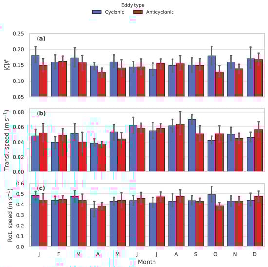
Figure 6.
Gulf-wide monthly variability for long-lived (>30 days) eddies: (a) normalized relative vorticity (), (b) translational speed, and (c) rotational speed. The letters on the horizontal axis denote the months of the year (January to December). Blue bars represent cyclonic eddies, and red bars represent anticyclonic eddies. Bars represent monthly mean values derived from track-averaged properties; error bars indicate 95% confidence intervals.
The interannual percentage of eddy tracks (Figure 7a) shows a near symmetric balance between cyclonic and anticyclonic eddies, with most years hovering near a 50/50 split. The monthly fraction (Figure 7b) also shows a relatively balanced population, with a slight preference for anticyclones in spring (Mar–May) and a notable anticyclonic peak in September. This is offset by a strong cyclonic dominance in late summer (August) and mid-autumn (October), demonstrating that the system maintains a near symmetrical polarity balance overall. A chi-square goodness-of-fit test applied to the aggregate long-lived population confirmed that the deviation from a 50/50 polarity split (98 cyclones vs. 110 anticyclones) is not statistically significant (), supporting the overall symmetry of the census.
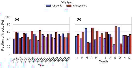
Figure 7.
Fraction of long-lived (>30 days) cyclonic (blue) and anticyclonic (red) tracks by (a) year and (b) month. The Gulf-wide population maintains a stable interannual and seasonal polarity balance.
3.4. SSHA–SSTA Relationship
The relationship between dynamic height (SSHA) and surface thermal expression (SSTA) was examined using a Gulf-wide daily correlation (Figure 8) and spatial climatologies (Figure 9).
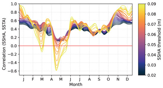
Figure 8.
Daily SSHA–SSTA correlation for the entire Gulf of California (2010–2024). Line color indicates the SSHA amplitude threshold used for the calculation. The solid red line indicates zero correlation. The strong positive winter correlation breaks down and reverses sign in spring (April–May).
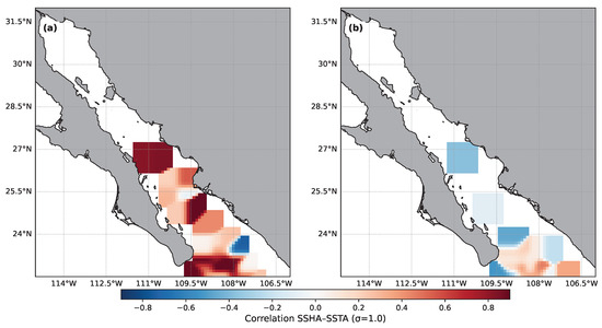
Figure 9.
Spatial distribution of the correlation between SSHA and SSTA within detected eddy tracks. (a) January:Represents the winter regime with strong positive coupling (red), consistent with the thermal wind balance where cyclones have cold cores. (b) May: Represents the spring transition, showing a breakdown of correlation and the emergence of negative values (blue), illustrating the seasonal thermal masking effect driven by surface heating. The correlation fields are smoothed () for visualization.
The Gulf-wide daily correlation coefficient was computed by taking the instantaneous spatial correlation between the daily SSHA and SSTA fields. The time-series (Figure 8) displays multiple correlation curves where the line color indicates a minimum SSHA amplitude threshold applied to the detection of the features. This technique ensures that the correlation is calculated exclusively over regions of strong mesoscale activity. The color bar confirms that the calculation includes features with SSHA amplitudes from to .
During the cold season (November through February), the correlation is strongly positive (>0.8), suggesting a robust coupling where cyclonic eddies correspond to cold surface anomalies and anticyclones to warm anomalies, consistent with baroclinic structures. This coupling is spatially coherent across the southern basins, as illustrated in the January map (Figure 9a), where high positive correlation values are ubiquitous along the eddy tracks.
However, this coupling breaks down rapidly in spring (March–April) and dramatically reverses in May, when correlations become negative (<−0.6). This reversal indicates that cyclonic eddies (dynamically low SSHA) are associated with warmsurface anomalies (positive SSTA) during this period. The spatial distribution in May (Figure 9b) confirms that this is a basin-wide phenomenon, showing a collapse of the coherent signal and the emergence of negative correlations in the regions of high eddy activity..
This reversal suggests a transient thermal–dynamical decoupling, driven by the intense seasonal heat flux into the Gulf [39]. This intense surface heating forms a shallow seasonal thermocline that overwhelms or ’caps’ the dynamic cold-core signature at the surface, a mechanism well-documented in the region [40]. The coupling begins to re-establish in summer (Jun–Aug) before strengthening back to the winter state in autumn.
3.5. Case Study: Long-Lived and Quasi-Stationary Eddies
The properties of the ten longest-lived eddy tracks identified by the algorithm are detailed in Table 4 and mapped in Figure 10. These persistent structures provide insight into the retentive features of the Gulf.
Table 4.
Top-10 longest eddy tracks (Gulf-wide, ≥30 days) given by the start and end dates.
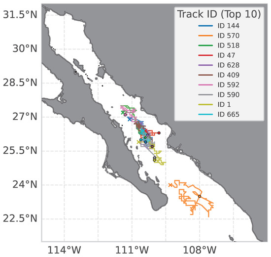
Figure 10.
Trajectories of the ten longest-lived eddies detected in the Gulf of California (2010–2024). Solid lines indicate the path of each eddy centroid, with circles (○) denoting start of detection and crosses (✕) indicating the end of detection. Colors correspond to unique Track IDs listed in the legend. Note the predominant confinement in the southern deep basins, with some trajectories (e.g., ID 570) exhibiting northward propagation.
A clear pattern emerges: all ten of the longest-lived tracks are located in the southern Gulf (south of N). Nine of these ten are cyclonic. These eddies are characterized by extreme lifetimes (211–516 days), with two tracks (ID 144 and 570) exceeding one year. Their behavior is not uniform; the trajectories reveal two dominant behaviors. First, strong topographic trapping is evident for the most persistent eddies (e.g., Track 144, blue, and Track 47, red), where the start (○) and end (✕) positions are geographically close, indicating confinement within a single deep basin (Guaymas or Farallon) for their entire duration.
Second, other trajectories display significant meridional displacement and inter-basin connectivity. In particular, eddies such as Track 570 (orange) and Track 518 (green) exhibit a clear net northward component, with their final positions located poleward relative to their initial positions (Figure 10). This suggests that while topography acts as a retention mechanism, interaction with background currents can drive coherent structures across basin sills, promoting meridional connectivity across adjacent basins.
Given the extreme 516-day lifetime of Track ID 144, a diagnostic analysis was performed (Figure 11) to verify that this was a single event and not a “false merger” tracking error. This continuity is strongly supported by our tracking methodology, which employs a multi-parameter cost function heavily penalizing polarity changes () and using a gradual gap penalty (Table 1), making accidental merging of unrelated features highly unlikely. The time-series of vorticity, amplitude, and diameter (Figure 11) confirm that it is a continuous, single, and coherent structure that evolves seasonally, strengthening significantly in summer 2014 before weakening. This analysis confirms that under favorable conditions, quasi-stationary eddies can be trapped in the deep southern basins for periods exceeding one year. This diagnostic also supports the interpretation that the meridional displacement observed in other long-lived tracks reflects genuine propagation rather than tracking artifacts.
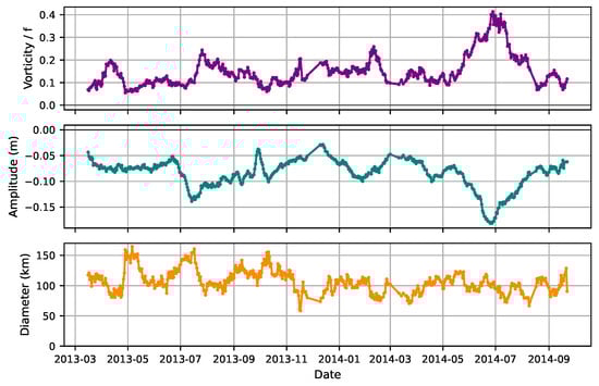
Figure 11.
Diagnostic time series for Track ID 144 (lifetime 516 days). From top to bottom: normalized vorticity (), SSHA amplitude (m), and median diameter (km). The continuous signal in all panels, with only minor gaps (≤2 days), confirms it is a single, evolving eddy and not a tracking error.
4. Discussion
4.1. Performance and Robustness of the Hybrid Framework
A fundamental question for any regional census is the necessity of a new detection framework given the existence of established global eddy atlases (e.g., [34,41]). While these global products are invaluable for open-ocean dynamics, their algorithms are configured for broad-scale features and often perform poorly in topographically complex, narrow marginal seas like the GC. Their methods can struggle with coastal interactions, spurious detections near islands, and the different physical scales of eddies, leading to fragmented tracks and unreliable statistics. Therefore, a regional framework was required.
Our hybrid detector addresses this by merging the geometric sensitivity of the closed-contour method [1] with the dynamical selectivity of the velocity geometry criterion [17]. This multi-criterion approach is a recognized strategy to enhance accuracy, improving upon the known limitations of single-criterion methods [42,43]. Furthermore, our tracking algorithm was specifically configured for the Gulf’s dynamics. This involved optimizing the cost function to prioritize spatial proximity and polarity over noisy daily parameters, a practice consistent with other regional tracking studies [35]. Our work thus contributes to the growing body of research using new high-resolution datasets to resolve eddy dynamics in complex coastal and marginal seas [44,45].
The performance metrics presented in this study demonstrate the advantages of this approach. The CHE11 method alone, while sensitive, suffers from low precision in this region due to coastal noise. In contrast, the NEN10 method, when strictly evaluated, showed limitations in determining polarity within the Gulf’s complex constraints. We acknowledge that, in the absence of a comprehensive independent validation dataset, the hybrid catalog itself served as the reference baseline for this performance assessment. The robustness of this framework is further supported by the alignment of our statistical outputs (e.g., diameters, rotational speeds) with historical in-situ and observational literature. Although the final catalog is presented in a binary accepted/rejected form, detection confidence is implicitly encoded through the multi-criterion filtering and the temporal persistence required for track acceptance. Crucially, the identified long-lived eddies exhibit amplitudes and spatial scales well within the core of the parameter space (significantly exceeding the minimum thresholds), rendering them insensitive to minor uncertainties in the detection criteria.
Despite its robustness, the method has limitations. The reliance on fixed thresholds for amplitude ( m) and circularity () may exclude genuine, albeit weak or highly deformed, eddies. The circularity threshold was specifically adjusted to 0.5 to retain coherent eddies during deformation (e.g., coastal interaction), which proved essential for reducing artificial track fragmentation. Similarly, the 15-day maximum gap, chosen to bridge a 1.5×altimetric repeat cycle [36], was critical for tracking quasi-stationary structures but carries a small risk of merging successive, unrelated eddies. Future work could explore adaptive thresholds to refine this balance. In practice, long-lived trajectories exhibit consistent geometric properties over time (as shown in the diagnostic case study), supporting identity continuity despite intermittent detectability.
We also acknowledge that applying uniform detection thresholds across the entire domain may introduce a bias in the census, particularly in the northern Gulf where dynamics are distinct. However, sensitivity tests indicated that lowering the amplitude threshold (e.g., <2 cm) to capture weaker northern features approached the instrument’s error margin. This compromise resulted in detections that were indistinguishable from sensor noise, significantly compromising data reliability. Furthermore, adjusting geometric parameters specifically for the northern Gulf did not yield a robust separation between signal and noise without introducing artifacts. Consequently, we prioritized a conservative, uniform approach to ensure the reliability of the catalog, confirming that the observed contrast—a transient high-frequency North versus a persistent, eddy-rich South—is a robust physical feature rather than a methodological artifact. The resolution of these high-frequency northern dynamics likely requires the sub-mesoscale resolving capabilities of the SWOT mission.
4.2. Gulf Dynamics: Two Distinct Regimes
Our results reveal two distinct dynamical regimes in the Gulf’s mesoscale circulation, separated by the Midriff Islands. Our analysis, focused on persistent mesoscale structures (>30 days), identified a limited number of such tracks in the northern Gulf (). This finding is consistent with the census of [16], who reported that, while the northern basin is dynamically active, the vast majority of its mesoscale features are transient, with typical lifespans of only 1–11 days. By imposing a 30-day persistence threshold, our census effectively filters out this ephemeral population, confirming that the high mesoscale activity in the North is fundamentally different from the long-lived nature of the South.
However, historical hydrographic studies have also described coherent seasonal gyres in the northern basins that persist for months [46,47]. The fact that these stable features are not resolved as continuous tracks in our census likely reflects the challenges of satellite altimetry in this tidally resonant region. Although standard tidal corrections are applied to the source data, the northern Gulf is known for its extreme tidal energy [48]. In such regions, residual tidal errors can manifest as high-frequency aliasing in the SSHA signal, which may fragment the tracks of slower-evolving seasonal gyres or mask their geostrophic signature against the background noise. Therefore, our results suggest that while the northern Gulf supports intense transient activity and seasonal circulation, its persistent mesoscale eddies are likely underestimated by altimetry due to signal-to-noise limitations.
In contrast, the southern basins (Guaymas, Carmen, Pescadero) function as an effective trap for persistent eddies. Our census shows median lifetimes of 52.5–60 days in this region, confirming the stable, topographically constrained nature of these eddies described in the literature [7]. One relevant finding is the persistence of quasi-stationary eddies, with lifetimes exceeding one year. Our diagnostic analysis confirms these are single, coherent structures rather than tracking artifacts. This observed behavior is consistent with strong bathymetric trapping, where the deep basins shelter the eddies from strong mean advection. This provides observation-based evidence of multi-year topographic trapping, a phenomenon in which eddies are constrained by the bathymetry of deep basins, as explored in numerical simulations by [18] and suggested in previous models [47,49].
In contrast, a subset of other long-lived eddies (such as Track ID 570) demonstrate significant inter-basin connectivity. These trajectories exhibit a predominant poleward propagation, characterized by a net northward displacement relative to their initial detection. This behavior is physically consistent with the advection of the seasonally intense Mexican Coastal Current, which flows north during summer and autumn [8,14]. This implies that the southern Gulf operates not merely as a retention zone, but as an active exchange system where coherent structures can transport biogeochemical properties up-basin, overcoming local topographic trapping. This dynamic behavior is not captured by lifetime statistics alone and only becomes evident through a full trajectory analysis.
This persistence is dominated by cyclonic eddies, which account for 9 of the 10 longest-lived tracks. This suggests a dynamic preference related to the conservation of potential vorticity over the Gulf’s deep basins [37]. The bottom topography acts as a trapping mechanism, and vortex stretching—as the water column is vertically extended or held stable over the deep basins—favors the stability and longevity of cyclonic structures () [1].
4.3. Seasonal Variability and Generation Mechanisms
The seasonal analysis of the eddy population reveals a bimodal pattern in intensity and rotational speed, with peaks in winter and late summer. This variability aligns with the two primary forcing regimes of the Gulf. The winter peak corresponds to the period of maximum wind stress, where strong northwesterly winds drive intense surface circulation and coastal upwelling events [8]. These wind-driven instabilities likely contribute to the generation of energetic eddies during the cold season.
Conversely, the secondary peak observed in late summer and autumn is consistent with the intensification of the poleward-flowing Mexican Coastal Current. As demonstrated by numerical studies [14], the interaction of this coastally trapped current with the abrupt topography of the eastern coast (e.g., capes and ridges) is a primary mechanism for the generation of eddy trains in the southern Gulf. The fact that our census captures these distinct seasonal signals in both vorticity and rotational speed confirms that the hybrid framework effectively resolves the response of the mesoscale field to both wind-driven and current-driven forcing mechanisms.
4.4. SSHA–SSTA Relationship and Seasonal Decoupling
The relationship between SSHA and SSTA provides information on the vertical structure of the eddies. For most of the year, the correlation is positive, consistent with the thermal quasi-geostrophic dynamics [37,38] where cyclones are cold and anticyclones are warm. This coupling is spatially robust across the southern basins during the winter peak, where high positive correlation values dominate the eddy tracks, confirming that the surface thermal signature accurately reflects the subsurface dynamics.
However, a significant finding is the reversal of this correlation in spring. This indicates a transient thermal-dynamical decoupling. Our analysis reveals that the spatially coherent signal collapses during this transition and shifts towards negative values, indicating that cyclonic eddies (low SSHA) develop a warmsurface signature (high SSTA). This phenomenon could be a direct consequence of the region’s intense seasonal heating, which creates a shallow, warm surface layer that “masks” or “caps” the dynamically induced cold core below [39,40]. However, in the southern region near the entrance, the persistence of positive correlations may be attributed to the intrusion of cooler California Current Water, which can mitigate this thermal masking effect, a process consistent with the circulation patterns described by [50,51]. This finding is critical because it demonstrates that eddy censuses in the GC based solely on SST would miss the majority cyclonic eddies during the spring transition. This result highlights the necessity of altimetry-based methods like SSHA for a complete census in coastal seas with strong seasonal stratification.
This work provides a consistent and physically grounded 14-year eddy census for the GC. This catalog is a novel resource for investigating the connectivity between basins, air-sea interactions, and regional energy budgets. By demonstrating the existence of multi-year quasi-stationary cyclonic eddies and characterizing the distinct regimes of the Gulf, this study provides a new baseline for understanding the region’s mesoscale variability. Because the procedures are formulated in physical units, they can be directly extended to other marginal seas or emerging high-resolution altimetry products, anticipating the requirements of the new generation of ocean observing systems.
5. Conclusions
This study demonstrates that a regionally configured hybrid framework is essential to resolve mesoscale dynamics in topographically complex marginal seas, overcoming the limitations of standard global eddy atlases. The resulting 14-year census reveals a fundamental partition in the GC: the northern Gulf is dominated by transient mesoscale activity, where persistent eddy detection is limited by strong tidal aliasing and signal-to-noise constraints, whereas the southern Gulf operates as a region of robust topographic trapping, supporting long-lived and even quasi-stationary cyclonic eddies persisting for over a year. Trajectory analysis further shows that, beyond local retention, a subset of long-lived eddies exhibits coherent poleward propagation consistent with advection by the seasonally intensified Mexican Coastal Current, indicating that this region also functions as an active exchange pathway capable of transporting properties up-basin—a behavior not captured by lifetime statistics alone. In addition, the documented seasonal decoupling between SSHA and SSTA highlights the limitations of SST-based eddy identification during spring heating, when surface warming masks the geostrophic signature of cyclones. Together, these results provide a physically grounded benchmark for mesoscale circulation in the GC and establish a scalable methodological foundation for exploiting the resolving capabilities of the new generation of swath altimetry missions, such as SWOT, in coastal and marginal seas.
Author Contributions
Conceptualization, Y.P.-C., H.T. and K.R.-M.; methodology, Y.P.-C. and H.T.; software, Y.P.-C. and H.T.; validation, Y.P.-C.; formal analysis, Y.P.-C.; investigation, Y.P.-C.; resources, H.T. and K.R.-M.; data curation, Y.P.-C.; writing—original draft preparation, Y.P.-C.; writing—review and editing, Y.P.-C., H.T. and K.R.-M.; visualization, Y.P.-C.; supervision, H.T. and K.R.-M.; project administration, K.R.-M. All authors have read and agreed to the published version of the manuscript.
Funding
The doctoral studies of Yuritzy Pérez-Corona were supported by a fellowship from the Secretariat of Science, Humanities, Technology and Innovation (SECIHTI), Government of Mexico (CVU 995804).
Data Availability Statement
The NeurOST dataset [20] is publicly available at https://doi.org/10.5067/NEURO-STV24 (accessed on 12 January 2026). The MUR SST dataset [23] is available at https://doi.org/10.5067/GHGMR-4FJ04 (accessed on 12 January 2026). The complete Python code used for this study is available on GitHub (v1.0) at https://github.com/YuritzyPC/eddy-detection-tracking-paper (accessed on 12 January 2026). The output data catalogs generated and analyzed during this study are publicly archived on Zenodo at https://doi.org/10.5281/zenodo.17409704 (accessed on 12 January 2026). These catalogs, provided in NetCDF and CSV formats, include: (1) eddy_detections_hybrid_GoC_2010_2024.nc, containing all daily eddy detections; (2) tracks_catalog_full.nc, containing all 971 raw trajectories; and (3) tracks_catalog_min14d.nc, containing the filtered 344 coherent trajectories with ≥14 detections.
Acknowledgments
This research was conducted during the Ph.D. studies of Yuritzy Pérez-Corona at the Centro de Investigación Científica y de Educación Superior de Ensenada (CICESE). During the preparation of this work, the authors used ChatGPT-4 (OpenAI) to assist with Python code development and debugging. After using ChatGPT, the authors reviewed and edited the content as needed and take full responsibility for the content of the publication. H.T. acknowledges the support of the Jet Propulsion Laboratory, California Institute of Technology under a prime contract with NASA (80NM0018D0004), and was awarded under NASA Research Announcement (NRA) NNH23ZDA001N-SWOTST, NASA Surface Water and Ocean Topography (SWOT) Science Team.
Conflicts of Interest
The authors declare no conflicts of interest. The funders had no role in the design of the study; in the collection, analyses, or interpretation of data; in the writing of the manuscript; or in the decision to publish the results.
Abbreviations
The following abbreviations are used in this manuscript:
| DUACS | Data Unification and Altimeter Combination System |
| EKE | Eddy Kinetic Energy |
| GC | Gulf of California |
| MUR | Multi-scale Ultra-high Resolution |
| NeurOST | Neural Ocean Surface Topography |
| SLA | Sea Level Anomaly |
| SSH | Sea Surface Height |
| SSHA | Sea Surface Height Anomaly |
| SST | Sea Surface Temperature |
| SSTA | Sea Surface Temperature Anomaly |
| SWOT | Surface Water and Ocean Topography |
References
- Chelton, D.B.; Schlax, M.G.; Samelson, R.M. Global observations of nonlinear mesoscale eddies. Prog. Oceanogr. 2011, 91, 167–216. [Google Scholar] [CrossRef]
- Morrow, R.; Le Traon, P.Y. Recent advances in observing mesoscale ocean dynamics with satellite altimetry. Adv. Space Res. 2012, 50, 1062–1076. [Google Scholar] [CrossRef]
- Ferrari, R.; Wunsch, C. Ocean circulation kinetic energy: Reservoirs, sources, and sinks. Annu. Rev. Fluid Mech. 2009, 41, 253–282. [Google Scholar] [CrossRef]
- McWilliams, J.C. Submesoscale, coherent vortices in the ocean. Rev. Geophys. 1985, 23, 165–182. [Google Scholar] [CrossRef]
- Fu, L.L. Pattern and velocity of propagation of the global ocean eddy variability. J. Geophys. Res. Ocean. 2009, 114, C11017. [Google Scholar] [CrossRef]
- Argote, M.L.; Amador, A.; Lavin, M.F.; Hunter, J.R. Tidal dissipation and stratification in the Gulf of California. J. Geophys. Res. Ocean. 1995, 100, 16103–16118. [Google Scholar] [CrossRef]
- Lavín, M.F.; Marinone, S.G. An overview of the physical oceanography of the Gulf of California. In Nonlinear Processes in Geophysical Fluid Dynamics; Velasco-Fuentes, O.U., Sheinbaum, J., Ochoa, J., Eds.; Springer: Dordrecht, The Netherlands, 2003; pp. 173–204. [Google Scholar]
- Lavín, M.F.; Castro, R.; Beier, E.; Godínez, V.M. Mesoscale eddies in the southern Gulf of California during summer: Characteristics and interaction with the wind stress. J. Geophys. Res. Ocean. 2013, 118, 1367–1381. [Google Scholar] [CrossRef]
- GEBCO Compilation Group. GEBCO_2025 Grid—A Continuous Terrain Model of the Global Oceans and Land. 2025. Available online: https://doi.org/10.5285/34f8b6e8-0d73-6e7d-e063-093794aae8d2 (accessed on 12 January 2026).
- Fernández-Barajas, M.; Monreal-Gómez, M.; Molina-Cruz, A. Thermohaline structure and geostrophic flow in the Gulf of California, during 1992. Cienc. Mar. 1994, 20, 267–286. [Google Scholar] [CrossRef]
- Emilsson, I.; Alatorre, M. Evidencias de un remolino ciclónico de mesoescala en la parte sur del Golfo de California. Contrib. Oceanogr. Fís. México. Monogr. 1997, 3, 173–182. [Google Scholar]
- Pegau, W.S.; Boss, E.; Martínez, A. Ocean color observations of eddies during the summer in the Gulf of California. Geophys. Res. Lett. 2002, 29, 6-1–6-3. [Google Scholar] [CrossRef]
- Farach-Espinoza, E.B.; López-Martínez, J.; García-Morales, R.; Nevárez-Martínez, M.O.; Lluch-Cota, D.B.; Ortega-García, S. Temporal Variability of Oceanic Mesoscale Events in the Gulf of California. Remote Sens. 2021, 13, 1774. [Google Scholar] [CrossRef]
- Zamudio, L.; Hogan, P.; Metzger, E.J. Summer generation of the Southern Gulf of California eddy train. J. Geophys. Res. Ocean. 2008, 113, C06020. [Google Scholar] [CrossRef]
- Badan-Dangon, A.; Koblinsky, C.; Baumgartner, T. Spring and summer in the Gulf of California-observations of surface thermal patterns. Oceanol. Acta 1985, 8, 13–22. [Google Scholar]
- Lopez-Calderon, J.; Martinez, A.; Gonzalez-Silvera, A.; Santamaria-del Angel, E.; Millan-Nuñez, R. Mesoscale eddies and wind variability in the northern Gulf of California. J. Geophys. Res. Ocean. 2008, 113, C10001. [Google Scholar] [CrossRef]
- Nencioli, F.; Dong, C.; Dickey, T.; Washburn, L.; McWilliams, J.C. A Vector Geometry–Based Eddy Detection Algorithm and Its Application to a High-Resolution Numerical Model Product and High-Frequency Radar Surface Velocities in the Southern California Bight. J. Atmos. Ocean. Technol. 2010, 27, 564–579. [Google Scholar] [CrossRef]
- Costa de Almeida Tenreiro, M.J. Topographic Effects on the Formation, Evolution and Organization of Coherent Structures in Turbulent Flows: The Gulf of California Case. Ph.D. Thesis, Centro de Investigación Científica y de Educación Superior de Ensenada (CICESE), Ensenada, Baja California, Mexico, 2011. [Google Scholar]
- Martin, S.A.; Manucharyan, G.E.; Klein, P. Deep Learning Improves Global Satellite Observations of Ocean Eddy Dynamics. Geophys. Res. Lett. 2024, 51, e2024GL110059. [Google Scholar] [CrossRef]
- Martin, S.A.; Manucharyan, G.E.; Klein, P. Daily NeurOST L4 Sea Surface Height and Surface Geostrophic Currents. 2024. Available online: https://doi.org/10.5067/NEURO-STV24 (accessed on 12 January 2026).
- Morrow, R.; Fu, L.L.; Ardhuin, F.; Benkiran, M.; Chapron, B.; Cosme, E.; d’Ovidio, F.; Farrar, J.T.; Gille, S.T.; Lapeyre, G.; et al. Global Observations of Fine-Scale Ocean Surface Topography With the Surface Water and Ocean Topography (SWOT) Mission. Front. Mar. Sci. 2019, 6, 232. [Google Scholar] [CrossRef]
- Fu, L.L.; Ubelmann, C. On the transition from profile altimeter to swath altimeter for observing global ocean surface topography. J. Atmos. Ocean. Technol. 2014, 31, 560–568. [Google Scholar] [CrossRef]
- JPL MUR MEaSUREs Project. GHRSST Level 4 MUR Global Foundation Sea Surface Temperature Analysis. 2015. Available online: https://doi.org/10.5067/GHGMR-4FJ04 (accessed on 12 January 2026).
- Chin, T.M.; Vazquez-Cuervo, J.; Armstrong, E.M. A Multi-scale High-resolution Analysis of Global Sea Surface Temperature. Remote Sens. Environ. 2017, 200, 154–169. [Google Scholar] [CrossRef]
- Okubo, A. Horizontal dispersion of floatable particles in the vicinity of velocity singularities such as convergences. Deep Sea Res. Oceanogr. Abstr. 1970, 17, 445–454. [Google Scholar] [CrossRef]
- Weiss, J. The dynamics of enstrophy transfer in two-dimensional hydrodynamics. Phys. D Nonlinear Phenom. 1991, 48, 273–294. [Google Scholar] [CrossRef]
- Halo, I.; Backeberg, B.; Penven, P.; Ansorge, I.; Reason, C.; Ullgren, J.E. Eddy properties in the Mozambique Channel: A comparison between observations and two numerical ocean circulation models. Deep Sea Res. Part II Top. Stud. Oceanogr. 2014, 100, 38–53. [Google Scholar] [CrossRef]
- Isern-Fontanet, J.; García-Ladona, E.; Font, J. Identification of marine eddies from altimetric maps. J. Atmos. Oceanic Technol. 2003, 20, 772–778. [Google Scholar] [CrossRef]
- Jolliffe, I.T.; Cadima, J. Principal component analysis: A review and recent developments. Philos. Trans. R. Soc. A 2016, 374, 20150202. [Google Scholar] [CrossRef]
- Harasti, P.R.; Randall, D.A.; Toth, Z. Principal Component Analysis of Doppler Radar Data. Part I: Spatial Structures. J. Atmos. Sci. 2005, 62, 4271–4283. [Google Scholar] [CrossRef]
- Otsuka, H.; Ohta, Y.; Hino, R.; Kubota, T.; Inazu, D.; Inoue, T.; Takahashi, N. Reduction of non-tidal oceanographic fluctuations in ocean-bottom pressure records of DONET using principal component analysis to enhance transient tectonic detectability. Earth Planets Space 2023, 75, 112. [Google Scholar] [CrossRef]
- Chaigneau, A.; Eldin, G.; Dewitte, B. Eddy activity in the four major upwelling systems from satellite altimetry (1992–2007). Prog. Oceanogr. 2009, 83, 117–123. [Google Scholar] [CrossRef]
- Pegliasco, C.; Chaigneau, A.; Morrow, R. Main eddy vertical structures observed in the four major Eastern Boundary Upwelling Systems. J. Geophys. Res. Ocean. 2015, 120, 6008–6033. [Google Scholar] [CrossRef]
- Faghmous, J.H.; Frenger, I.; Yao, Y.; Warmka, R.; Lindell, A.; Kumar, V. A daily global mesoscale ocean eddy dataset from satellite altimetry. Sci. Data 2015, 2, 150028. [Google Scholar] [CrossRef]
- Trott, C.B.; Subrahmanyam, B.; Chaigneau, A.; Delcroix, T. Eddy Tracking in the Northwestern Indian Ocean During Southwest Monsoon Regimes. Geophys. Res. Lett. 2018, 45, 6594–6603. [Google Scholar] [CrossRef]
- Du, Y.; Zhang, Y.; He, P. Automated detection and tracking of mesoscale eddies in the South China Sea. Acta Oceanol. Sin. 2013, 32, 36–43. [Google Scholar] [CrossRef]
- Marshall, J.; Plumb, R.A. Atmosphere, Ocean and Climate Dynamics: An Introductory Text; International Geophysics; Academic Press: Burlington, MA, USA, 2008; Volume 93. [Google Scholar]
- Assassi, C.; Morel, Y.; Vandermeirsch, F.; Chaigneau, A.; Pegliasco, C.; Morrow, R.; Colas, F.; Fleury, S.; Carton, X.; Klein, P.; et al. An Index to Distinguish Surface- and Subsurface-Intensified Vortices from Surface Observations. J. Phys. Oceanogr. 2016, 46, 2529–2552. [Google Scholar] [CrossRef]
- Castro, R.; Lavín, M.F.; Ripa, P. Seasonal heat balance in the Gulf of California. J. Geophys. Res. Ocean. 1994, 99, 3249–3261. [Google Scholar] [CrossRef]
- Paden, C.A.; Abbott, M.R.; Winant, C.D. Tidal and atmospheric forcing of the upper ocean in the Gulf of California, 1. Sea surface temperature variability. J. Geophys. Res. Ocean. 1991, 96, 18337–18359. [Google Scholar] [CrossRef]
- Pegliasco, C.; Delepoulle, A.; Mason, E.; Morrow, R.; Faugère, Y.; Dibarboure, G. META3.1exp: A new global mesoscale eddy trajectory atlas derived from altimetry. Earth Syst. Sci. Data 2022, 14, 1087–1107. [Google Scholar] [CrossRef]
- Yi, J.; Du, Y.; He, Z.; Zhou, C. Enhancing the accuracy of automatic eddy detection and the capability of recognizing the multi-core structures from maps of sea level anomaly. Ocean Sci. 2014, 10, 39–48. [Google Scholar] [CrossRef]
- Xing, T.; Yang, Y. Three Mesoscale Eddy Detection and Tracking Methods: Assessment for the South China Sea. J. Atmos. Ocean. Technol. 2021, 38, 243–258. [Google Scholar] [CrossRef]
- Erickson, Z.K.; Fields, E.; Johnson, L.; Thompson, A.F.; Dove, L.A.; D’Asaro, E.; Siegel, D.A. Eddy Tracking From In Situ and Satellite Observations. J. Geophys. Res. Ocean. 2023, 128, e2023JC019701. [Google Scholar] [CrossRef]
- Zhang, X.; Liu, L.; Fei, J.; Li, Z.; Wei, Z.; Zhang, Z.; Jiang, X.; Dong, Z.; Xu, F. Advances in surface water and ocean topography for fine-scale eddy identification from altimeter sea surface height merging maps in the South China Sea. Ocean Sci. 2025, 21, 1033–1045. [Google Scholar] [CrossRef]
- Carrillo, L.; Lavín, M.; Palacios-Hernández, E. Seasonal evolution of the geostrophic circulation in the northern Gulf of California. Estuar. Coast. Shelf Sci. 2002, 54, 157–173. [Google Scholar] [CrossRef]
- Marinone, S.G. A three-dimensional model of the mean and seasonal circulation of the Gulf of California. J. Geophys. Res. Ocean. 2003, 108, 3325. [Google Scholar] [CrossRef]
- Palacios-Hernández, E.; Argote, M.; Amador, A.; Morales-Pérez, R. Summer-autumn mean surface circulation in the northern Gulf of California. Deep Sea Res. Part II Top. Stud. Oceanogr. 2002, 49, 4275–4289. [Google Scholar]
- Beier, E. A numerical investigation of the annual variability in the Gulf of California. J. Phys. Oceanogr. 1997, 27, 615–632. [Google Scholar] [CrossRef]
- Godínez, V.M.; Beier, E.; Lavín, M.F.; Kurczyn, J.A. Circulation at the entrance of the Gulf of California from satellite altimeter and hydrographic observations. J. Geophys. Res. Ocean. 2010, 115, C04007. [Google Scholar] [CrossRef]
- Pantoja, D.A.; Marinone, S.G.; Parés-Sierra, A.; Gómez-Valdivia, F. Numerical modeling of seasonal and mesoscale hydrography and circulation in the Mexican Central Pacific. Cienc. Mar. 2012, 38, 663–676. [Google Scholar] [CrossRef]


Disclaimer/Publisher’s Note: The statements, opinions and data contained in all publications are solely those of the individual author(s) and contributor(s) and not of MDPI and/or the editor(s). MDPI and/or the editor(s) disclaim responsibility for any injury to people or property resulting from any ideas, methods, instructions or products referred to in the content. |
© 2026 by the authors. Licensee MDPI, Basel, Switzerland. This article is an open access article distributed under the terms and conditions of the Creative Commons Attribution (CC BY) license.