Weighted Total Variation for Hyperspectral Image Denoising Based on Hyper-Laplacian Scale Mixture Distribution

Highlights

What are the main findings?

• Proposes a Hyper-Laplacian Scale Mixture prior for HSI gradient modeling.
• Introduces a region-adaptive weighted total variation model for HSI denoising.

What are the implications of the main findings?

• Improves denoising performance in both smooth and textured regions with better texture preservation.
• Achieves state-of-the-art performance and can enhance other TV-based methods when integrated.

Abstract

Conventional total variation (TV) regularization methods based on Laplacian or fixed-scale Hyper-Laplacian priors impose uniform sparsity penalties on gradients. These uniform penalties fail to capture the heterogeneous sparsity characteristics across different regions and directions, often leading to the over-smoothing of edges and loss of fine details. To address this limitation, we propose a novel regularization Hyper-Laplacian Adaptive Weighted Total Variation (HLAWTV). The proposed regularization employs a proportional mixture of Hyper-Laplacian distributions to dynamically adapt the sparsity decay rate based on image structure. Simultaneously, the adaptive weights can be adjusted based on local gradient statistics and exhibit strong robustness in texture preservation when facing different datasets and noise. Then, we propose an hyperspectral image (HSI) denoising method based on the HLAWTV regularizer. Extensive experiments on both synthetic and real hyperspectral datasets demonstrate that our denoising method consistently outperforms state-of-the-art methods in terms of quantitative metrics and visual quality. Moreover, incorporating our adaptive weighting mechanism into existing TV-based models yields significant performance gains, confirming the generality and robustness of the proposed approach.

1. Introduction

Hyperspectral images acquire data across hundreds of contiguous spectral bands, enabling detailed characterization of real-world scenes through rich spectral and spatial information. This makes hyperspectral images indispensable in a variety of applications, including anomaly detection [1], environmental monitoring [2], military surveillance [3], precision agriculture [4], and object detection [5]. However, during the acquisition process, HSI is often corrupted by various noise types such as Gaussian noise, impulse noise, stripe noise, and deadlines. These mixed noises significantly deteriorate the image quality and adversely affect subsequent processing tasks [6,7,8,9]. Therefore, robust and efficient denoising techniques are essential to enhance the reliability of hyperspectral images in practical scenarios.

An intuitive approach is to treat each band of a hyperspectral image as an individual grayscale image and directly apply traditional grayscale denoising algorithms, such as non-local means (NLM) [10], block-matching 3D filtering (BM3D) [11], and weighted nuclear norm minimization (WNNM) [12]. However, these methods ignore the spectral correlations of HSI. To solve this problem, some algorithms process the entire hyperspectral data as a 3D cube, such as block-matching 4D filtering (BM4D) [13] and video block-matching 4D filtering (V-BM4D) [14]. However, without prior constraints on the inherent characteristics of HSI, it is difficult to achieve optimal denoising performance. Consequently, researchers have begun developing denoising methods that exploit spectral correlations and spatial structures. These methods are generally categorized into two classes as follows: (1) Deep learning-based methods directly learn mapping functions between noisy and clean HSI pairs from training datasets to avoid explicit modeling of prior knowledge. (2) Prior model-based methods formulate HSI denoising as a constrained optimization problem by incorporating hyperspectral priors such as low-rankness in the spectral dimension, local smoothness in the spatial domain, and self-similarity of pixel patches.

In recent years, deep learning–based hyperspectral image denoising has advanced from simple spatial–spectral convolutional neural networks (CNNs) to more sophisticated architectures that effectively balance local and global context. HSID-CNN [15] pioneered the use of deep residual convolution with multiscale and multilevel feature fusion to suppress noise while preserving spectral–spatial consistency. QRNN3D [16] introduced alternating-direction quasi-recurrent pooling alongside 3D convolutions to model both spatio-spectral correlations and global spectral dependencies simultaneously. More recently, SSRT-UNet [17] integrated non-local spatial self-similarity and global spectral correlation within a single recurrent transformer U-Net block, enabling unified exploitation of hyperspectral priors across shift-window layers. TRQ3DNet [18] combined 3D quasi-recurrent blocks with U-Transformer modules connected via a bidirectional integration bridge, capturing both local textures and long-range dependencies and delivering state-of-the-art denoising performance. ILRNet [19] integrates the strengths of model-driven and data-driven approaches by embedding a rank minimization module within a U-Net architecture. However, these deep learning models still face significant limitations. Their performance heavily relies on paired clean–noisy datasets and assumed noise priors, which hinders their adaptability in real-world scenarios where such datasets are not available, or the noise characteristics may differ significantly. This reliance on prior knowledge and training on specific datasets restricts the generalization capability of these models when exposed to complex or unseen noise types, highlighting a key challenge in applying them to diverse and unstructured real-world noise conditions.

Prior model-based approaches for hyperspectral image denoising have attracted significant attention due to their flexibility and strong interpretability. Rather than relying on large-scale annotated datasets, these methods explicitly incorporate various types of prior knowledge about hyperspectral images, such as low-rankness and local smoothness. By leveraging these priors, model-based methods can adapt more effectively to different noise types and complex real world scenarios.

Among these priors, low-rankness has proven especially useful for modeling the strong spectral correlation inherent in hyperspectral data. Building upon this idea, Zhang et al. proposed the low-rank matrix recovery (LRMR) framework [20], which exploits spectral low-rank priors to suppress noise. However, methods based solely on low-rank tend to overlook spatial structure information, resulting in suboptimal performance when dealing with complex noise such as stripes or structured artifacts.

To address the above problem, spatial smoothness priors have been introduced. For example, He et al. incorporated TV regularization [21] in their low-rank matrix denoising (LRTV) method [22], applying both low-rankness and local smoothness to better preserve spatial details and enhance denoising performance. Nevertheless, this method requires unfolding hyperspectral data into matrices, which can destroy the intrinsic spatial structure. To overcome this limitation, recent methods have modeled hyperspectral images as 3D tensors. For example, LRTDTV [23] combines Tucker decomposition with spatial–spectral TV (SSTV) [24] to effectively remove complex noise. However, balancing the parameters between low-rank and smoothness regularizations remains challenging. Recognizing that low-rank regularization is often coupled with smoothness priors, Wang et al. [25] further proposed directly imposing low-rank constraints on gradient tensors to encode both low-rankness and local smoothing simultaneously within the tensor framework. This formulation improves the adaptivity and representation power of total variation regularization across different structural patterns in hyperspectral images. To improve the texture preserving capability of TV regularization, some methods introduce adaptive weighting strategies for sparsity constraints across spatial and spectral directions. For example, Anisotropic Spectral Spatial TV (ASSTV) [26] uses anisotropic full variability in three directions, which explores HSI spectral continuity and spatial smoothing while taking into account the directionality of the texture. Graph Spatio-Spectral TV (GSSTV) [27] weights the spatial difference operator of SSTV based on a graph reflecting the spatial structure of the HSI image, which can better respond to the spatial structure of the image. However, most of these weighting schemes apply the same sparsity constraint to every pixel, causing textured areas to be over-smoothed since they ignore local gradient variations. To solve this problem, Chen et al. proposed a TPTV regularizer [28] with gradient map weighting $l_1$-parameter. The gradient map is utilized to adaptively adjust the weights so as to reduce the sparsity constraints on pixels with large variations.

In recent years, Hyper-Laplacian TV (HLTV) methods have garnered significant attention because they can more accurately model the peaky nature and heavy-tailed characteristics of spatial–spectral gradients in hyperspectral images compared to traditional Laplacian TV (LTV) [29,30]. However, although both LTV and HLTV approaches strive to equation the regularization with the true sparse distribution of gradients, current TV-based denoising methods still have the following problems in hyperspectral image denoising:

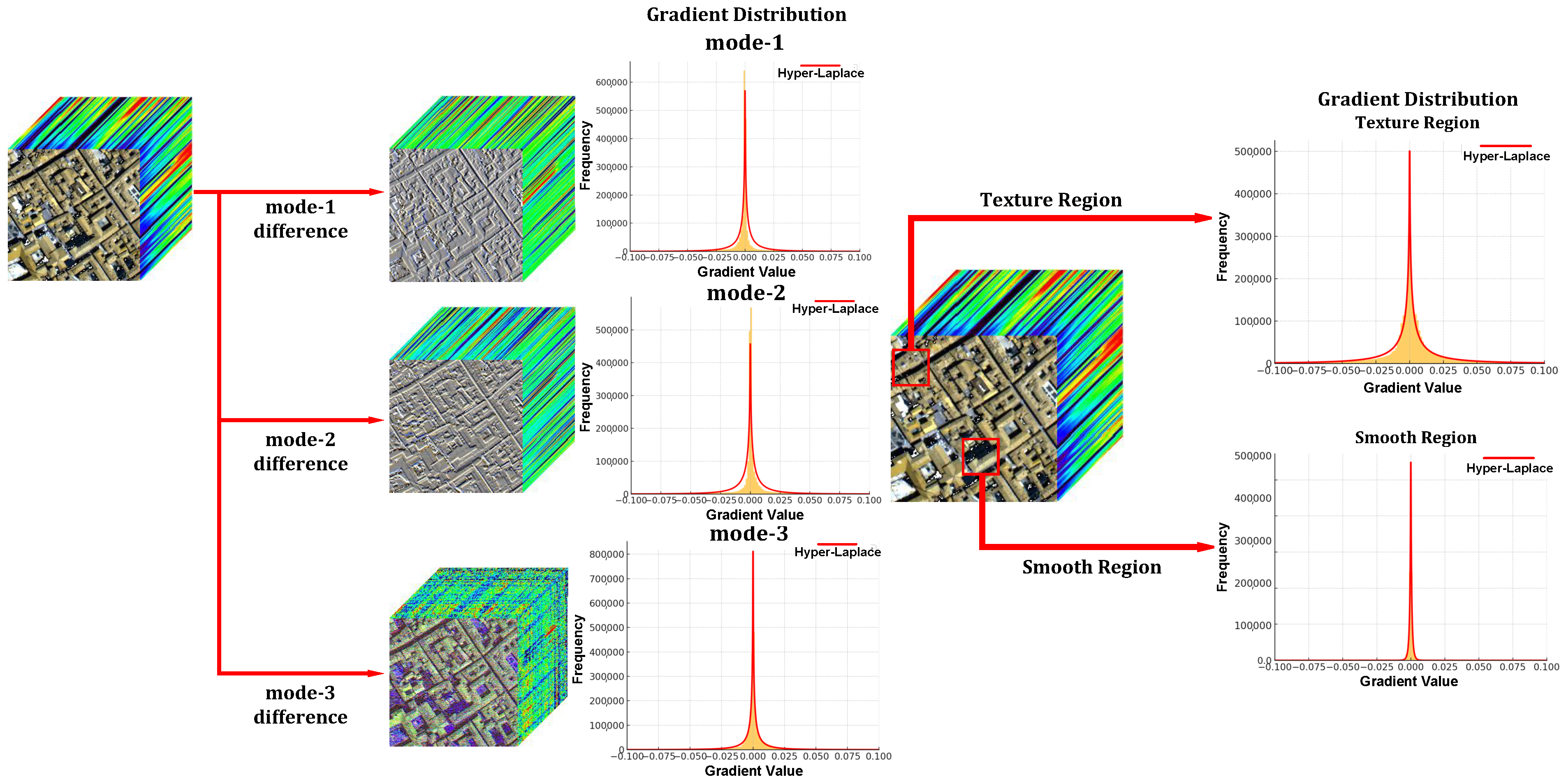
(1) Existing HLTV regularizers use a fixed $l_p$-norm constraint for each gradient direction, implicitly assuming that gradients originating from smooth areas or richly textured regions, follow the same heavy-tailed distribution. In reality, hyperspectral images exhibit markedly different gradient statistics across spatial versus spectral dimensions and between smooth versus textured regions as shown in Figure 1. By ignoring this heterogeneity, HLTV regularization fails to capture the true prior distribution of the data. As a result, it often over-smooths details in textured areas, leading to suboptimal noise removal.

(2) Although LTV models introduce heuristic weight functions to protect edges and textures, these weights are typically fixed mappings derived from simplified priors. They lack the flexibility to adapt dynamically to local gradient characteristics. Consequently, such models struggle to discriminate effectively between flat regions and highly textured ones as follows: over-smoothing may be introduced in flat regions, while insufficient protection is provided in highly textured regions, resulting in the underutilization of the sparsity feature of HSI gradients. In addition, such heuristics are difficult to adaptively set reasonable weight sizes based on the statistical properties of HSI, thus limiting the overall regularization performance.

Based on the above observations, we propose a novel HLAWTV regularization method, which is built upon a Hyper-Laplacian Scale Mixture (HLSM) distribution model. Our method assumes that gradients in hyperspectral images follow Hyper-Laplacian distributions with different scales in smooth and textured regions. We embed this assumption into a maximum a posteriori (MAP) estimation framework, which yields an adaptive weighted regularization term. Specifically, the regularization fits variable-scale Hyper-Laplacian distributions based on both the direction-specific gradient statistics and the magnitude of local gradient values, enabling the model to control the sparsity decay rate dynamically. This model improves the adaptivity of total variation regularization across different structural patterns in hyperspectral images.

The main contributions of this article can be summarized as follows.

(1) We propose a sparse prior modeling method based on the Hyper-Laplacian scale mixture distribution to more accurately characterize the statistical properties of hyperspectral image gradients. Specifically, considering that the HSI gradients usually exhibit distribution patterns with varying degrees of spiking and heavy tailing in different directions, we model them using a variable scale super-Laplacian distribution. To further introduce regional adaptation, we derive a probabilistic scale mixture model by exploiting the prior conjugacy of the Hyper-Laplacian distribution with the gamma distribution.

(2) Based on the HLSM distribution, we further propose a new weighted total variation regularization model HLAWTV. To efficiently solve the resulting optimization problem, we develop a tailored algorithm based on the Alternating Direction Method of Multipliers (ADMM), which achieves effective and scalable denoising performance.

(3) Experimental results demonstrate that the proposed denoising method performs better than other advanced methods. Furthermore, migration experiments show that the denoising performance can be significantly improved by embedding our weighting scheme into existing TV regularizers.

The rest of this article is organized as follows. The second part gives signs and preliminary knowledge. The third part introduces the HLSM distribution model, HLAWTV regularizer, and denoising model. The fourth part reports the experimental results. The fifth part is the conclusion.

2. Preliminaries

2.1. Notations

We summarize notations used in this article in

Table 1. Notation declarations.

Notations	Interpretations
$x,\mathbf{x},\mathrm{X},\mathcal{X}$	scalar, vector, matrix, tensor
$\mathcal{X}\in {\mathbb{R}}^{I_1\times I_2\times \cdots \times I_N}$	Nth-order tensor
$x_{i_1,i_2,\dots ,i_N}$	element at position $(i_1,i_2,\dots ,i_N)$ of $\mathcal{X}$
${\parallel \mathcal{X}\parallel }_1$	${\displaystyle {\sum }_{i_1,i_2,\dots ,i_N}\left|x_{i_1,i_2,\dots ,i_N}\right|}$
${\parallel \mathcal{X}\parallel }_q$	${\displaystyle \sqrt[q]{{\sum }_{i_1,i_2,\dots ,i_N}{\left|x_{i_1,i_2,\dots ,i_N}\right|}^q}}$

. Next, we introduce the definitions of mode-n unfolding, the mode-k tensor-matrix product, and the mode-k gradient map.

The n-mode unfolding of N-order tensors can be divided into horizontal unfolding ${\mathrm{X}}_{\left(n\right)}\in {\mathbb{R}}^{I_1\dots I_{n-1}{I}_{n+1}\dots I_N}$ and vertical unfolding ${\mathrm{X}}^{\left(n\right)}\in {\mathbb{R}}^{I_1\dots I_{n-1}{I}_{n+1}\dots I_N}$.

The mode-k tensor-matrix product of a tensor $\mathcal{X}\in {\mathbb{R}}^{I_1\times I_2\times \cdots \times I_n}$ and a matrix $\mathrm{A}\in {\mathbb{R}}^{J_1\times I_k}$ is defined as follows:

$$\mathcal{Y}=\mathcal{X}{\times }_k\mathrm{A}.k=1,2,3$$

(1)

The gradient map of $\mathcal{X}\in {\mathbb{R}}^{I_1\times I_2\times I_3}$ along mode-k can be denoted as ${\mathcal{G}}_k\left(\mathcal{X}\right)$, which is defined as follows:

$${\mathcal{G}}_k\left(\mathcal{X}\right)={\nabla }_k\left(\mathcal{X}\right)=D_k\mathcal{X},k=1,2,3,$$

(2)

where $D_k$ represent the first-order finite difference operators.

2.2. The Laplacian Scale Mixture Distribution

A random variable $s_i$ is said to follow a Laplacian Scale Mixture (LSM) distribution if it can be expressed as follows:

$$s_i={\lambda }_i^{-1}{u}_i,$$

(3)

where $u_i$ is a Laplacian random variable with the following unit scale:

$$p\left(u_i\right)={\displaystyle \frac{1}{2}}{e}^{-|u_i|},$$

(4)

and ${\lambda }_i$ is a positive random variable with density $p\left({\ge }_i\right)$. We assume $u_i$ and ${\lambda }_i$ are independent. Conditioned on ${\lambda }_i$, the distribution of $s_i$ becomes a Laplacian with inverse scale ${\lambda }_i$ as follows:

$$p\left(s_i\right|{\lambda }_i)={\displaystyle \frac{{\lambda }_i}{2}}{e}^{-{\lambda }_i\left|s_i\right|}.$$

(5)

Therefore, the marginal distribution of $s_i$ is an infinite mixture of Laplacians with different scales as follows:

$$p\left(s_i\right)={\int }_0^{\infty }p(s_i\mid {\lambda }_i)p\left({\lambda }_i\right)d{\lambda }_i={\int }_0^{\infty }{\displaystyle \frac{{\lambda }_i}{2}}{e}^{-{\lambda }_i\left|s_i\right|}p\left({\lambda }_i\right)d{\lambda }_i.$$

(6)

2.3. TV Regularizatiers

TV regularizatiers methods have emerged in hyperspectral image restoration, such as the early proposed 3-D TV model [23], the subsequent improved Enhanced 3-D TV (E3DTV) [31], and the correlated TV model [32]. To facilitate the subsequent analysis, we abstract and generalize their structures and use a unified representation framework to represent the above different TV regularizations as follows:

$${∥\mathcal{X}∥}_{3DTV}={∥D_1\mathcal{X}∥}_1+{∥D_2\mathcal{X}∥}_1+{∥D_3\mathcal{X}∥}_1,$$

(7)

where $\mathcal{X}$ is the mathematical representation of HSIs in different TV regularization models.

2.4. HSI Degradation Model

Since HSIs are often contaminated with various types of noise, the degradation model is typically represented as follows:

$$\mathcal{Y}=\mathcal{X}+\mathcal{E},$$

(8)

where the tensor $\mathcal{Y}$ represents the observed hyperspectral image, the tensor $\mathcal{X}$ represents the clean HSI, and the tensor $\mathcal{E}$ is the noise term. The goal of HSI denoising is to estimate the clean image $\mathcal{X}$ using the corrupted image $\mathcal{Y}$. The denoising model for HSIs can be represented as

$$\begin{array}{c}\begin{array}{c}\underset{\mathcal{X},\mathcal{E}}{\mathrm{arg\; min}}{\displaystyle \frac{1}{2}}{∥\mathcal{Y}-\mathcal{X}-\mathcal{E}∥}_F^2+\eta J_1\left(\mathcal{X}\right)+\lambda J_2\left(\mathcal{E}\right),\end{array}\hfill \end{array}$$

(9)

where the first term is the data fidelity term, the second term is used to describe the prior information of the clean HSI [33,34,35], and the third term is used to describe the sparsity of the mixed noise.

3. Methodology

In this section, we propose the HLAWTV regularizer and give its technical details, then propose a denoising model based on the HLAWTV regularizer, and finally utilize the ADMM algorithm to solve the denoising model.

3.1. HLSM Model

Different TV regularizers allow flexibility in balancing denoising and texture preservation capabilities by selecting different forms of $\mathcal{X}$. In traditional regularization frameworks, the $l_1$-norm is widely used to constrain the sparsity of the gradient map, implicitly assuming that the gradient map follows a fixed-scale LSM distribution [36,37] with probability density function (PDF) $p(x;\lambda )\propto e^{-\lambda \left|x\right|}$. However, some recent research has found that both spatial and spectral gradients in natural images exhibit significantly more heavy-tailed distributions. Specifically, their heavy-tailed distributions are closer to the Hyper-Laplacian distribution with probability density function $p(x;\lambda )\propto e^{-{\lambda \left|x\right|}^{{\alpha }_k}}$, where ${\alpha }_k$ controls the strength of the sparsity in that direction. A smaller ${\alpha }_k$ represents a stronger sparse prior.

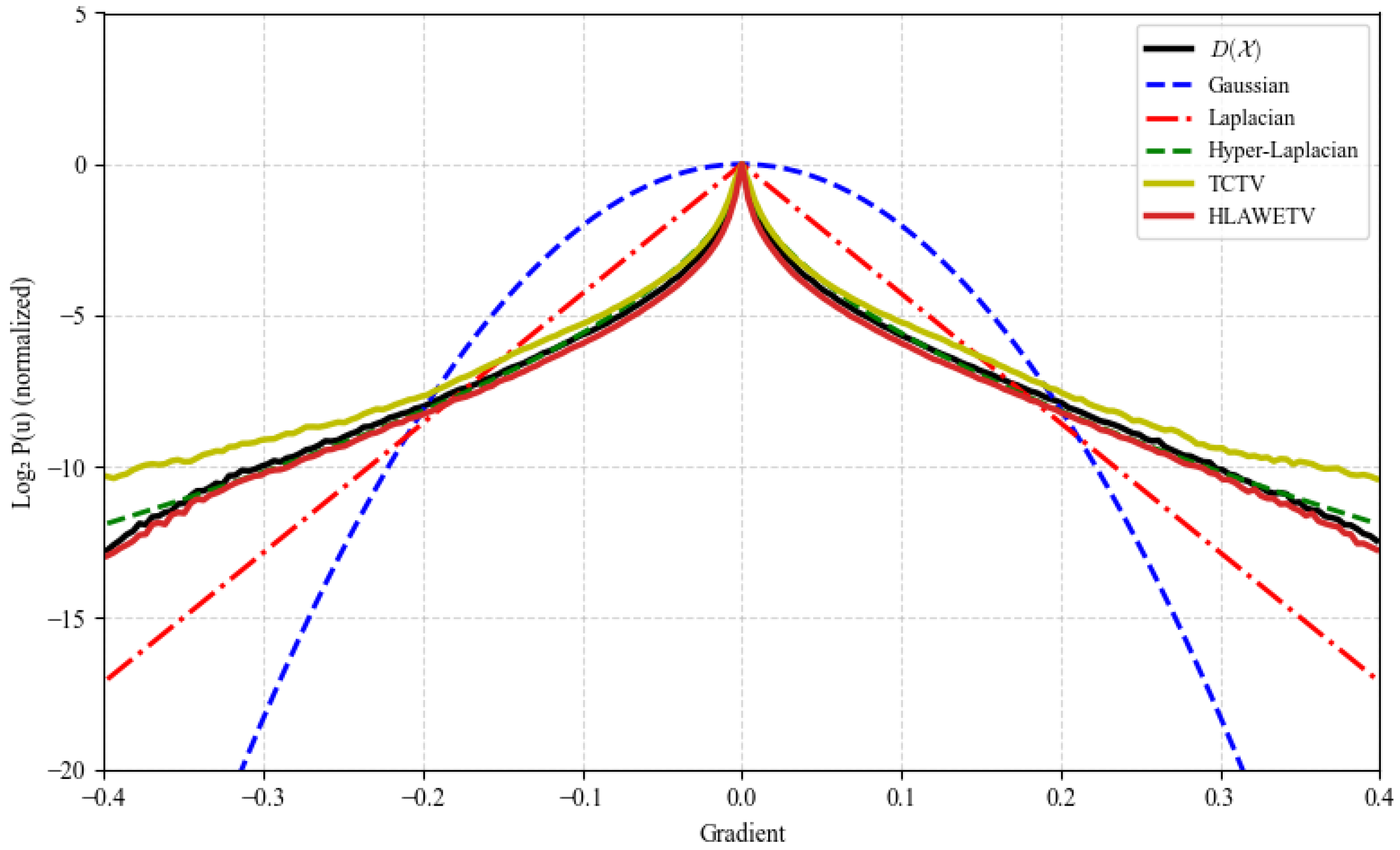
Based on the above theory, we propose a Hyper-Laplacian scale mixture distribution model. Current TV regularization based on the Hyper-Laplacian distribution assumes that the gradient values in the same difference direction independently and identically obey the Hyper-Laplacian distribution of the same scale. However, different regions of HSIs often have completely different structural characteristics. To better capture the nonstationary and sparse nature of gradient variations, we assume that the gradient values at each pixel point follow an independent distribution of the HLSM model. As shown in Figure 2, the methods based on HLSM distribution model closely matches the gradient distribution of $\mathcal{X}$. Specifically, for each pixel-wise gradient value ${\mathcal{G}}_{i,j,b}$, we assume the following model:

$$p\left({\mathcal{G}}_{i,j,b}\right)=\prod _{i,j,b}p\left({\mathcal{G}}_{i,j,b}\right).$$

(10)

Instead of assuming a LSM distribution, we define the following:

$$\begin{array}{c}p\left({\mathcal{G}}_{i,j,b}\right)=\int p({\mathcal{G}}_{i,j,b}\mid {\Theta }_{i,j})p\left({\Theta }_{i,j}\right)d{\Theta }_{i,j}\\ p({\mathcal{G}}_{i,j,b}\mid {\Theta }_{i,j})={\displaystyle \frac{{\alpha }_k{\Theta }_{i,j}}{2}}{\left|{\mathcal{G}}_{i,j,b}\right|}^{{\alpha }_k-1}exp\left(-{\Theta }_{i,j}{\left|{\mathcal{G}}_{i,j,b}\right|}^{{\alpha }_k}\right),\end{array}$$

(11)

where $0<{\alpha }_k<1$ is a sparsity-controlling exponent, allowing stronger sparsity than the Laplacian distribution (which corresponds to $\alpha =1$).

Since the integral form of $p\left({\mathcal{G}}_{i,j,b}\right)$ does not yield a closed-form solution, we adopt an Expectation-Maximization (EM) strategy to optimize the marginal log-likelihood $\ln \left(p\right(\mathcal{G}\left)\right)$.

E step: We compute the evidence lower bound (ELBO) of the log-marginal probability, given the current estimate ${\mathcal{G}}_{\left(t\right)}$. The ELBO is denoted as follows:

$$Q(\mathcal{G},{\mathcal{G}}^{\left(t\right)})=\int \prod _{i,j}p({\Theta }_{i,j}\mid {\mathcal{G}}^{\left(t\right)})ln\prod _{i,j,b}p({\mathcal{G}}_{i,j,b}\mid {\Theta }_{i,j})d{\Theta }_{i,j}.$$

(12)

Using the form of the Hyper-Laplacian conditional distribution, the optimization problem can be reformulated as follows:

$$Q(\mathcal{G},{\mathcal{G}}^{\left(t\right)})=-\sum _{i,j,b}\langle {\Theta }_{i,j}\rangle ·{\left|{\mathcal{G}}_{i,j,b}\right|}^{{\alpha }_k}+const,$$

(13)

where $\langle {\Theta }_{i,j}\rangle =W(i,j)$ is the expectation of ${\Theta }_{i,j}$ under the current posterior estimate. $W(i,j)$ is a function of ${\mathcal{G}}^{\left(t\right)}$. ${\alpha }_k=f({\mu }_k,{\sigma }_k)$. Both $W(i,j)$ and $f({\mu }_k,{\sigma }_k)$ will be discussed later. In practice, we assume that the posterior $p({\Theta }_{i,j}\mid {\mathcal{G}}^{\left(t\right)})$ obeys a Gamma distribution, or use local statistics to approximate it.

3.2. HLAWTV Regularizer with HLSM

M step: We maximize the ELBO w.r.t. $\mathcal{G}$, resulting in the following optimization:

$${\mathcal{G}}^{(t+1)}=arg\underset{\mathcal{G}}{min}\sum _{i,j,b}W(i,j)·{\left|{\mathcal{G}}_{i,j,b}\right|}^{{\alpha }_k}.$$

(14)

Consequently, following the optimization structure induced by the EM algorithm, we define the HLAWTV regularization term as follows:

$$\begin{array}{cc}\hfill {\parallel \mathcal{Z}\parallel }_{\mathrm{HLAWTV}}& =\sum _{k=1}^3{∥D_k\mathcal{X}∥}_{{\alpha }_k,W}\hfill \\ \hfill & =\sum _{k=1}^3\sum _{m,n,b}{W}_k(i,j)·{\left|{\mathcal{G}}_k(i,j,b)\right|}^{{\mathrm{ff}}_k}.\hfill \end{array}$$

(15)

In this way, incorporating HLAWTV as the regularization term is equivalent to maximizing the joint log-likelihood of the gradient priors along all directions, formulated as follows: $-{\sum }_{i=1}^{3}ln\left(p\left({\mathcal{G}}_i^{\mathcal{X}}\right)\right)$. This demonstrates that the adoption of HLAWTV serves not only as a regularization strategy but also as a probabilistic modeling of gradients, grounded in a prior-driven MAP estimation framework.

In our denoising framework, the adaptive weight map W plays a crucial role by acting as the scale parameter in the HLSM. Rather than assuming a fixed scale, we adopt a spatially adaptive formulation where W reflects the local structural complexity of the HSI. Because this scale parameter is a latent variable in HLSM, it is inherently unknown and its value is influenced by local spatial characteristics. To make W more data-adaptive, we explicitly design $W(i,j)$ to approximate this latent scale, effectively linking the statistical sparsity prior with image-driven structural information. In particular, large weights correspond to stronger contractions to ensure sparsity in the smoothing region, while small weights preserve larger gradient magnitudes in texture or edge regions.

To robustly estimate $W(i,j)$, we use low-rank filtering to obtain denoising estimates for hyperspectral images, which reduces the interference of noise in weight calculation. HSI exhibits consistent texture patterns across all bands, whereas the noise in each band is random. In order to extract the texture region of HSI more accurately, we use mean filtering along the spectral dimension to obtain a gradient map with better texture detail quality. The calculation formula is as follows:

$$G_k={\displaystyle \frac{1}{B}}\sum _{b=1}^B{\left({\mathcal{G}}_k\right)}_{(:,:,b)},k=1,2,3$$

(16)

where $G_k(i,j)$ is a matrix that provides a more reliable characterization of texture structures along the three modes of HSIs. To enhance the adaptivity of the regularization strength across different image regions, we use the Gamma distribution as a hyperprior over the scale parameter ${\Theta }_{i,j}$ in the HLSM as follows:

$$p\left({\Theta }_i\right)=(b^a/\Gamma \left(a\right)){\Theta }_i^{a-1}{e}^{-b{\Theta }_i}.$$

(17)

This choice is justified on multiple grounds as follows: (1) The gamma distribution is conjugate to the exponential family, enabling tractable marginalization. (2) By adjusting the shape parameter a and inverse scale parameter b, the gamma distribution flexibly models diverse behavioral characteristics ranging from strong sparsity to weak sparsity. In our method, the weighting scheme originates from Bayesian inference under the gamma-exponential conjugate model. Specifically, when the prior distribution of ${\Theta }_{i,j}$ is gamma and the conditional probability of ${\mathcal{G}}_{i,j,b}$ follows a Hyper-Laplacian distribution with inverse scale ${\Theta }_{i,j}$, the posterior probability of ${\Theta }_{i,j}$ given ${\mathcal{G}}_{i,j,b}$ is also gamma. This conjugacy allows us to directly update the posterior distribution of latent variables via the E-step of the EM algorithm as shown in Equation (13). Therefore, the posterior distribution of ${\Theta }_{i,j}$ is computed based on the current gradient ${\mathcal{G}}_{i,j,b}$ and remains a Gamma distribution as follows:

$${\Theta }_k|G_k\sim Gamma(a+1,b+|G_k\left|\right).$$

(18)

The expectation of this posterior yields the following adaptive weight function:

$$W_k(i,j)=\mathbb{E}\left[{\Theta }_{i,j}\right|G_k(i,j)]={\displaystyle \frac{a+1}{b+|G_k(i,j)|}}.$$

(19)

The proposed weighting function is monotonically decreasing in $G_k(i,j)$, which directly supports a sparse-modeling prior, as follows: when $|G_k(i,j)|\to 0$ in smooth regions, the weight becomes large to encourage smoothing; when $G_k(i,j)$ is large at edges or textures, the weight decreases to preserve fine details. Additionally, this weighting scheme improves robustness against noise, mitigating instability caused by gradient fluctuations.

3.3. Proposed Model

To better characterize the spatial–spectral structures of hyperspectral images, we propose a novel denoising model that integrates spectral subspace representation with the HLAWTV regularizer. By projecting the HSI gradient tensor into the spectral subspace, we are able to utilize the inherent spectral redundancy to suppress noise and maintain structural consistency across bands. This subspace representation improves denoising robustness while maintaining computational efficiency and is a strong complement to our proposed HLAWTV. Therefore, the spectral gradient of HSIs can be expressed as follows:

$${\mathcal{D}}_k\left(\mathcal{X}\right)={\mathcal{U}}_k{\times }_3{{\mathrm{V}}_k}^T,$$

(20)

where ${\mathcal{U}}_k\in {\mathbb{R}}^{M\times N\times r}$ contains the corresponding spatial coefficients, and ${\mathrm{V}}_k\in {\mathbb{R}}^{B\times r}$ is the spectral basis. This transformation allows the spatial variation across bands to be compactly encoded in ${\mathcal{U}}_i$. We use the HLAWTV regularizer to constrain ${\mathcal{U}}_i$ to enhance both sparsity and adaptivity across different spatial regions and gradient directions. Based on the above discussion, our proposed HLAWTV denoising model can be expressed as follows:

$$\begin{array}{c}\hfill \begin{array}{c}\underset{\mathcal{X},\mathcal{E},{\mathcal{U}}_k,{\mathrm{V}}_k}{\mathrm{arg\; min}}{\displaystyle \frac{1}{2}}{∥\mathcal{Y}-\mathcal{X}-\mathcal{E}∥}_F^2+\lambda {\displaystyle \sum _{k=1}^3}\parallel {\mathcal{U}}_k{\parallel }_{\mathrm{HLAWTV}}+{\parallel \mathcal{E}\parallel }_1\\ {\mathcal{D}}_k\left(\mathcal{X}\right)={\mathcal{U}}_k{\times }_3{{\mathrm{V}}_k}^T\\ {\mathrm{V}}_k^T{\mathrm{V}}_k=I.k=1,2,3\end{array}\end{array}$$

(21)

3.4. Algorithm

The proposed HSI denoising model is solved using ADMM. According to the ADMM method, the optimization problem described in Equation (21) can be solved by minimizing the following augmented Lagrangian function:

$$\begin{array}{c}\begin{array}{c}\begin{array}{cc}\hfill \mathcal{L}(\mathcal{X},\mathcal{E},{\mathcal{U}}_k,{\mathcal{V}}_k,{\mathcal{M}}_k)=& \lambda \sum _{k=1}^3{∥{\mathcal{U}}_k∥}_{{\alpha }_k,W}+{\parallel \mathcal{E}\parallel }_1\hfill \\ \hfill & +\sum _{k=1}^3{\displaystyle \frac{\mu }{2}}{\parallel {\mathcal{D}}_k\left(\mathcal{X}\right)-{\mathcal{U}}_k{\times }_3{\mathrm{V}}_k^T+{\displaystyle \frac{{\mathcal{M}}_k}{\mu }}\parallel }_F^2\hfill \\ \hfill & +{\displaystyle \frac{\mu }{2}}{\parallel \mathcal{Y}-\mathcal{X}-\mathcal{E}+{\displaystyle \frac{{\mathcal{M}}_4}{\mu }}\parallel }_F^2,\hfill \end{array}\end{array}\hfill \end{array}$$

(22)

where ${\mathcal{M}}_k$ (k = 1, 2, 3) and ${\mathcal{M}}_4$ are Lagrange multipliers. $\mu$ is the penalty parameter. Each variable can be updated alternatively, while the other variables remain constant.

(1) Update ${\mathcal{U}}_k$ and ${\mathrm{V}}_k$: The subproblem with respect to ${\mathcal{U}}_i$ can be expressed as

$$\begin{array}{c}\hfill \underset{{\mathcal{U}}_k}{min}\lambda {∥{\mathcal{U}}_i∥}_{{\alpha }_k,W}+{\displaystyle \frac{\mu }{2}}{∥{\mathcal{D}}_k\left(\mathcal{X}\right)+{\displaystyle \frac{{\mathcal{M}}_k}{\mu }}-{\mathcal{U}}_k{\times }_3{\mathrm{V}}_k∥}_F^2.\end{array}$$

(23)

For each directional gradient tensor ${\mathcal{D}}_k$, we first unfold the 3D tensor into a 2D matrix to facilitate subspace modeling as follows:

$${\mathrm{D}}_k=\mathrm{Unfold}\left({\mathcal{D}}_k\left(\mathcal{X}\right)\right)\in {\mathbb{R}}^{MN\times B}.$$

(24)

Then, the update of the subspace coefficient matrix ${\mathrm{U}}_k$ is obtained by solving the following:

$$\underset{{\mathrm{U}}_k}{min}{\displaystyle \frac{\mu }{2}}{∥{\mathrm{D}}_k+{\displaystyle \frac{{\mathrm{M}}_k}{\mu }}-{\mathrm{U}}_k{\mathrm{V}}_k^{\top }∥}_F^2+\lambda {\parallel {\mathrm{U}}_k\parallel }_{{\alpha }_k,\mathrm{W}},$$

(25)

where ${\mathrm{D}}_k,{\mathrm{U}}_k$ and ${\mathrm{M}}_k$ represent the mode-3 unfolding matrices of ${\mathcal{D}}_k,{\mathcal{U}}_k$ and ${\mathcal{M}}_k$. This problem is solved using the following two-step procedure:

In the first step, we update the matrices ${\mathrm{U}}_k^{\left(temp\right)}$ and ${\mathrm{V}}_k^{(t+1)}$ with Singular Value Decomposition (SVD) as follows:

$$\{{\mathrm{U}}_k^{\left(temp\right)},{\mathrm{V}}_k^{(t+1)}\}=\mathrm{SVD}\left({\mathrm{D}}_k+{\displaystyle \frac{1}{\mu }}{\mathrm{M}}_k\right).$$

(26)

In the second step, we perform weighted nonconvex shrinkage on ${\mathrm{U}}_k^{\left(temp\right)}$ to update ${\mathrm{U}}_k^{(t+1)}$ as follows:

$${\mathrm{U}}_k^{(t+1)}={\mathrm{Shrink}}_{{\displaystyle \frac{\lambda W_k}{\mu }}}^q\left({\mathrm{U}}_k^{\left(temp\right)}\right),$$

(27)

where ${\mathrm{Shrink}}^q(·)$ is a generalized shrankage/thresholding operator [38]. To set parameters that better alight with the sparsity characteristics of gradients in both spatial and spectral dimensions, we set the value of q as ${\alpha }_k$, shown in Equation (35).

(2) Update $\mathcal{E}$: The subproblem with respect to $\mathcal{E}$ can be expressed as

$$\begin{array}{cc}\hfill \underset{\mathcal{E}}{min}& {∥\mathcal{Y}-\mathcal{X}+{\displaystyle \frac{{\mathcal{M}}_4}{\mu }}-\mathcal{E}∥}_F^2+{\displaystyle \frac{1}{\mu }}{∥\mathcal{E}∥}_1.\hfill \end{array}$$

(28)

The solution of $\mathcal{E}$ can be computed using the following soft-thresholding operator:

$${\mathcal{E}}^{(t+1)}={\mathcal{E}}_{{\displaystyle \frac{1}{\mu }}}(\mathcal{Y}-\mathcal{X}+{\displaystyle \frac{{\mathcal{M}}_4}{\mu }}).$$

(29)

(3) Update $\mathcal{X}$: The subproblem with $\mathcal{X}$ respect to can be expressed as

$$\begin{array}{cc}\hfill \underset{\mathcal{X}}{min}& {∥\mathcal{Y}-\mathcal{E}+{\displaystyle \frac{{\mathcal{M}}_4}{\mu }}-\mathcal{X}∥}_F^2\hfill \\ \hfill & +\sum _{k=1}^3{∥{\mathcal{U}}_k{\times }_3{V}_k^T-{\displaystyle \frac{{\mathcal{M}}_k}{\mu }}-{\mathcal{D}}_k\left(\mathcal{X}\right)∥}_F^2.\hfill \end{array}$$

(30)

Optimizing the above problem can be considered as solving the following linear system:

$$\begin{array}{cc}\hfill \left(\mu I+\mu \sum _{k=1}^3{\mathcal{D}}_k^T{\mathcal{D}}_k\right)\mathcal{X}& =\mu (\mathcal{Y}-\mathcal{E})+{\mathcal{M}}_4\hfill \\ \hfill & +\mu \sum _{i=1}^3{\mathcal{D}}_k^T\left({\mathcal{U}}_k{\times }_3{V}_k^T-{\displaystyle \frac{{\mathcal{M}}_k}{\mu }}\right)\hfill \end{array}$$

(31)

where $D_k^T$ indicates the transpose of $D_k$. This quadratic problem has an analytic solution on the Fourier domain as follows:

$$\left\{\begin{array}{c}\mathcal{H}=\mathcal{Y}-\mathcal{E}+{\displaystyle \frac{{\mathcal{M}}_4}{\mu }}+{\sum }_{k=1}^3{\mathcal{D}}_k^T\left({\mathcal{U}}_k{\times }_3{V}_k-{\displaystyle \frac{{\mathcal{M}}_k}{\mu }}\right)\hfill \\ \mathcal{T}={\left|\mathcal{F}\right({\mathcal{D}}_1\left)\right|}^2+{\left|\mathcal{F}\left({\mathcal{D}}_2\right)\right|}^2+{\left|\mathcal{F}\left({\mathcal{D}}_3\right)\right|}^2\hfill \\ {\mathcal{X}}^{t+1}={\mathcal{F}}^{-1}\left({\displaystyle \frac{\mathcal{F}\left(\mathcal{H}\right)}{\mathbf{1}+\mathcal{T}}}\right)\hfill \end{array}\right.$$

(32)

where $\mathbf{1}$ represents the tensor with all elements as 1. $\mathcal{F}(·)$ denotes the Fourier transform operator, and ${|·|}^2$ represents the squared magnitude of the element.

(4) Update $W_k$: To solve this subproblem, we calculate the parameter ${\alpha }_k$ for each direction based on the mean and standard deviation of the current gradient. Specifically, for each direction, the calculation of ${\alpha }_k$ is broken down into several steps as follows:

First, we normalize the rank of the current low-rank approximation matrix as follows:

$$R={\displaystyle \frac{r_0-r_{min}}{r_{max}-r_{min}}}.$$

(33)

As the iteration proceeds, R represents the rank of the current low-rank approximation matrix. It is normalized based on the current rank $r_0$, and the minimum and maximum ranks $r_{min}$ and $r_{max}$. This normalization ensures that the adjustment of the sparsity penalty is based on the current rank, dynamically adjusting it during iterations. Next, we compute the penalty term based on the standard deviation ${\sigma }_k$ and mean ${\mu }_k$ of the gradient to fit the gradient distribution in different directions as follows:

$$P_k=exp\left(-{\displaystyle \frac{{\sigma }_k}{{\mu }_k+ϵ}}\right).$$

(34)

Combining the ratio R and the penalty term $P_k$, we calculate ${\alpha }_k$ using the following formula:

$${\alpha }_k=f({\mu }_{i,j},{\sigma }_{i,j})=(1-R{P}_k)·{\alpha }_{max}+R{P}_k·{\alpha }_{min}.$$

(35)

Using the calculated values ${\alpha }_k$ as the shape parameter a, we update the weight $W_k$ in each pixel $(i,j)$ for each direction. The weight update is given by the following:

$$W_k(i,j)={\displaystyle \frac{{\alpha }_k+1}{b+|G_k(i,j)|}}.$$

(36)

To stabilize the weights, we normalize them as follows:

$$W_k(i,j)={\displaystyle \frac{W_k(i,j)}{max\left(W_k(i,j)\right)}}.$$

(37)

The multipliers are updated as follows:

$$\left\{\begin{array}{c}{\mathcal{M}}_k^{(t+1)}={\mathcal{M}}_k^{\left(t\right)}+\mu \left({\mathcal{D}}_k\left(\mathcal{X}\right)-{\mathcal{U}}_k{\times }_3{V}_k^T\right),k=1,2,3\hfill \\ {\mathcal{M}}_4^{(t+1)}={\mathcal{M}}_4^{\left(t\right)}+\mu (\mathcal{Y}-\mathcal{X}-\mathcal{E}).\hfill \end{array}\right.$$

(38)

The specific process of the ADMM solver for HLAWTV is shown in Algorithm 1.

Algorithm 1 ADMM solver for HLAWTV

Require: Noisy HSI $\mathcal{Y}$; regularization $\lambda$; rank bounds $r_{min},r_{max}$; shape-parameter bounds ${\alpha }_{min},{\alpha }_{max}$ Ensure: Recovered HSI $\mathcal{X}$   1: $\mathcal{X}\leftarrow \mathcal{Y}$, $\mathcal{E}\leftarrow 0$, ${\mathcal{M}}_k\leftarrow 0$   2: $t\leftarrow 1$   3: while not converged do   4:     Update ${\mathcal{U}}_i,{\mathcal{V}}_i$ by Equations (23)–(27)   5:     Update $\mathcal{E}$ by Equation (29)   6:     Update $\mathcal{X}$ by Equation (32)   7:     Update $W_k$ by Equation (37)   8:     Update ${\mathcal{M}}_k$ by Equation (38)   9:     $t\leftarrow t+1$ 10: end while

4. Results

To validate the superiority of the proposed method, we conduct extensive comparative experiments on both synthetic and real HSI datasets. Our method is compared with the following thirteen classical or state-of-the-art methods: the QRNN3D [16] using the recurrent network to explore the spatial–spectral and the global correlation along the spectrum, the ILRNet [19] embedding a rank minimization module within a U-Net architecture to integrate the strengths of model-driven and data-driven approaches, the LRTV [22] applying the traditional 2-D total variation regularizer to each band independently, the LRTDTV [23] integrating the SSTV regularizer into a low-rank tensor decomposition framework, TCTV [25] considering the spectral correlation and sparsity prior on gradient tensor, E3DTV [31] adopting edge-preserving strategies to enhance spatial detail retention, RCTV [32] imposing TV regularization on representative low-rank coefficients, and ETPTV [28] introducing a texture-preserving weighted TV regularizer. In addition to TV-based models, we also consider the following low-rank- and non-local-based methods: TNN [35] employing a tensor nuclear norm to exploit global low-rankness, LRTF-DFR [39] introducing a dual-factor low-rank tensor decomposition with spatial regularization, HNN [40] using a two-dimensional frontal Haar wavelet transform to disentangle low- and high-frequencies, FastHyDe [41] combining spectral subspace projection with non-local denoising for high efficiency, and NGmeet [42] jointly leveraging global low-rank spectral subspace and non-local self-similarity through block matching and iterative refinement. The relationships and differences between the proposed method and the compared methods are presented in Table 2. All deep learning models are implemented in PyTorch 2.5.1 and trained on a workstation equipped with an Intel Xeon Platinum 8480+ CPU and Nvidia H800 GPU, using a batch size of 4. All traditional methods are implemented in MATLAB R2018b and executed on a workstation equipped with an Intel Core i5-12600KF processor (2.50 GHz) and 16 GB of RAM.

4.1. Synthetic Data Experiments

To ensure a fair and comprehensive comparison, we performed simulated experiments on two hyperspectral datasets with distinct spatial and spectral characteristics. The Pavia City Centre (PaviaC) dataset1 with a size of 200 × 200 × 80 and the Washington DC Mall (WDC) dataset2 whose size is 256 × 256 × 144. These two datasets can be regarded as ground-truth hyperspectral data, as they exhibit no perceptible noise. The pixel intensities of each spectral band are normalized to the range [0, 1]. To simulate realistic acquisition scenarios, we synthetically generate six types of noise and add them to the clean dataset.

Case 1: Each pixel was corrupted by additive i.i.d. Gaussian noise with a standard deviation of $\sigma$ = 0.1.

Case 2: non-i.i.d. Gaussian noise was simulated by adding i.i.d. Gaussian noise with different variances to each spectral band, where the SNR for each band was randomly selected from the range of [1, 15] dB.

Case 3: A mixture of Gaussian noise and impulse noise is added to each band. The Gaussian noise is added as Case 1. The percentage of impulse noise is set to 0.2.

Case 4: The impulse noise is added as in Case 3. Furthermore, 20% (PaviaC) or 30% (WDC) of the bands were randomly selected to add random stripes, with the number of corrupted columns ranging from 10 to 30. A total of 10% of the bands were randomly selected to simulate deadline noise, in which 5 to 25 rows were randomly chosen and set to zero to emulate dead sensor lines.

Case 5: The stripe noise and deadlines are added as Case 4. The percentage of impulse noise is set to 0.5 (PaviaC) and 0.3 (WDC).

Case 6: A mixture of Gaussian noise, impulse noise, stripe noise, and deadlines are added to each band. The Gaussian noise is added as Case 2. The stripe noise and deadlines are added as Case 4. The percentage of impulse noise is set to 0.2.

To ensure the statistical reliability of the experimental results, each denoising experiment was repeated 20 times for each noise case. The denoising performance was quantitatively evaluated using three metrics: mean peak signal-to-noise ratio (MPSNR) [43], mean structural similarity index (MSSIM) [44], and spectral angle mapper (SAM), which together reflect spatial fidelity, structural preservation, and spectral accuracy. Furthermore, the average runtime of each method was recorded to assess computational efficiency.

Quantitative Comparison: We present the MPSNR, MSSIM, MSAM, and the mean time values of 20 repetitive experiments obtained by all the compared methods in Table 3 and Table 4. It can be seen that deep-learning denoising methods perform less effectively than traditional machine-learning approaches in both the PaviaC and WDC datasets, mainly because the training dataset ICVL is not similar to these datasets. In Case 2, FastHyDe achieves excellent performance in terms of MPSNR and MSSIM. This is because FastHyDe transforms non-i.i.d. Gaussian noise into i.i.d. noise through whitening, which significantly simplifies the noise model. However, it underperforms the proposed method in other cases. As observed, the proposed HLAWTV achieves overall superior results over the compared methods under nearly all cases. In both PaviaC and WDC datasets, our algorithm still achieves optimal results with i.i.d. Gaussian noise and non-i.i.d Gaussian noise compared to the algorithm using Gaussian noise constraint terms. In the case of impulse noise and structural noise (stripe noise and deadlines), our algorithm has less performance degradation with noise enhancement compared to other TV regularization based methods. This is due to the ability of our HLAWTV regularizer to adaptively adjust the sparse penalty strength based on structural information in different regions and directions.

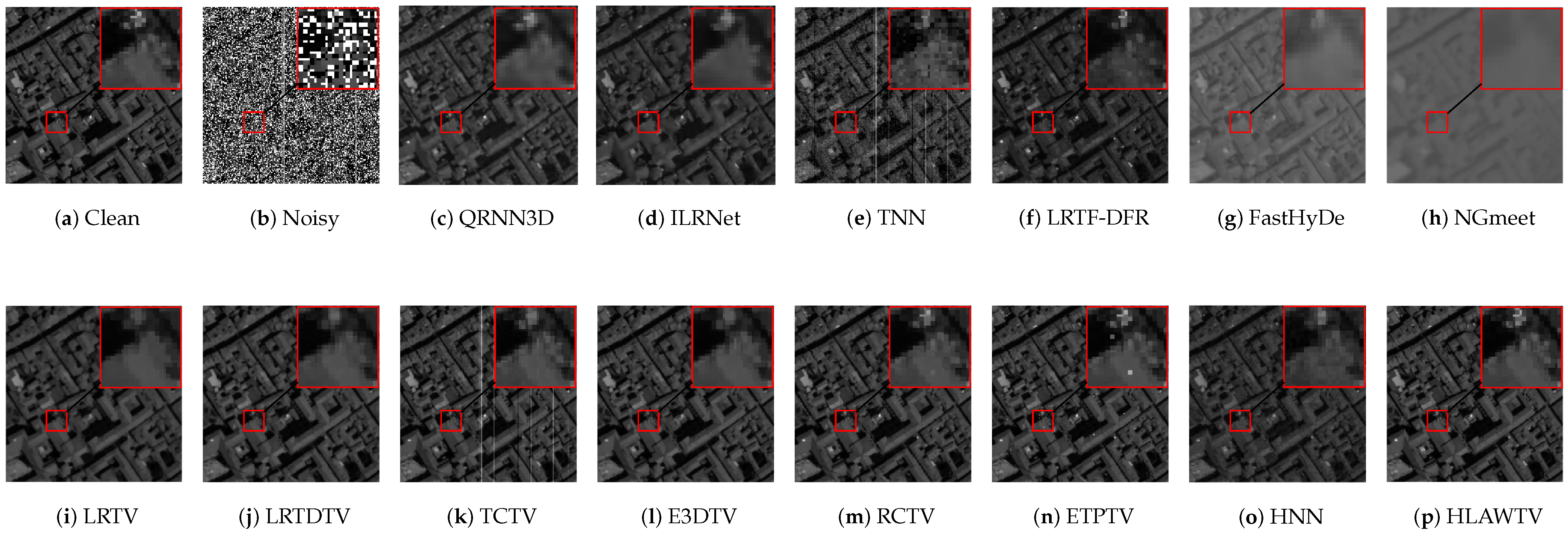
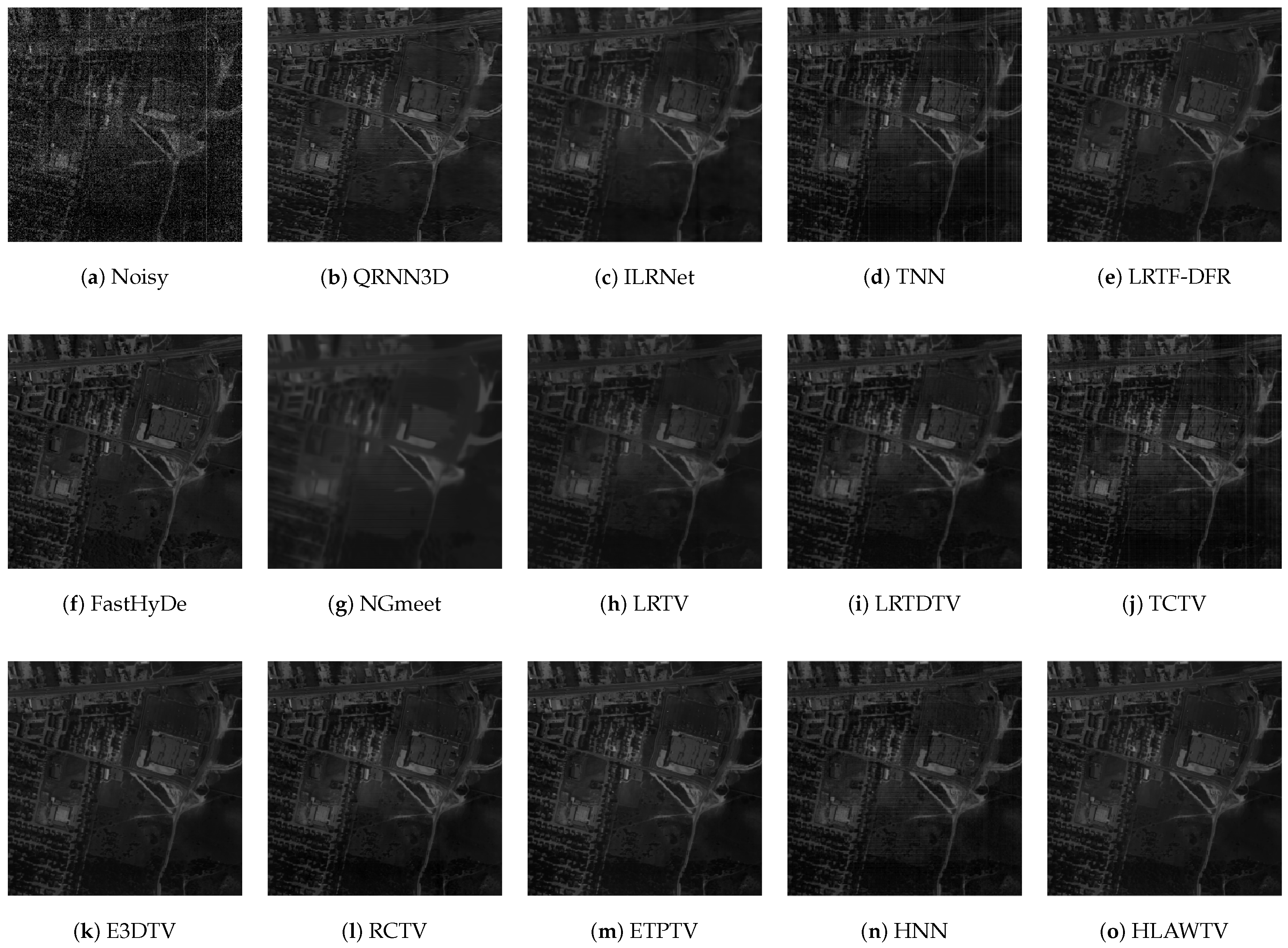
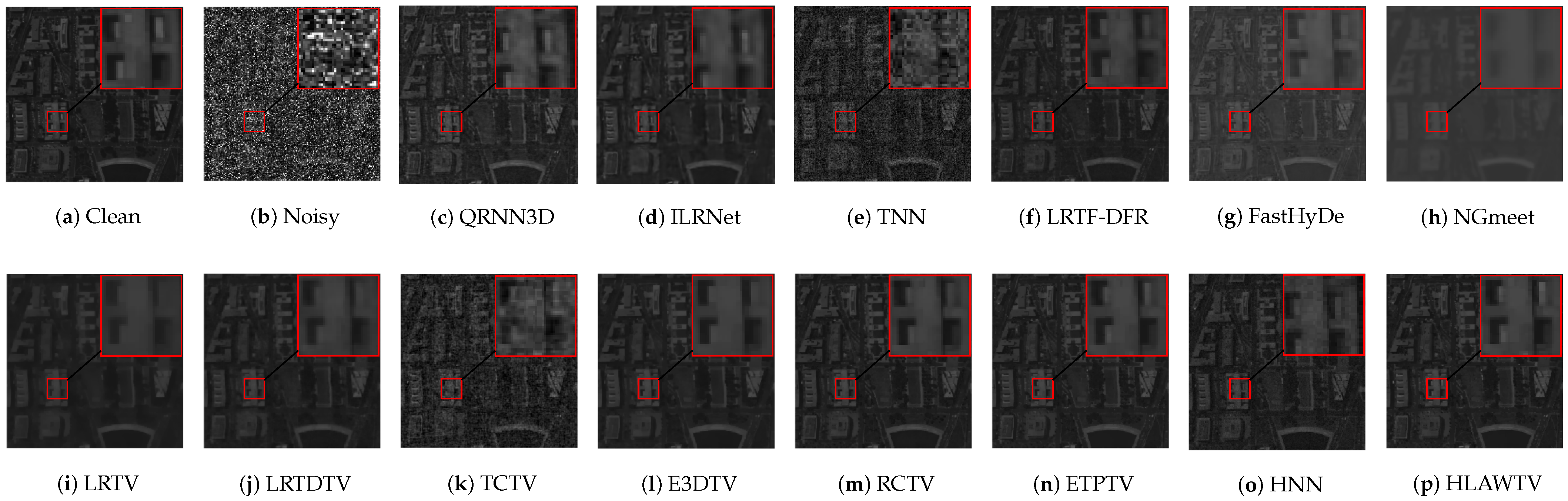
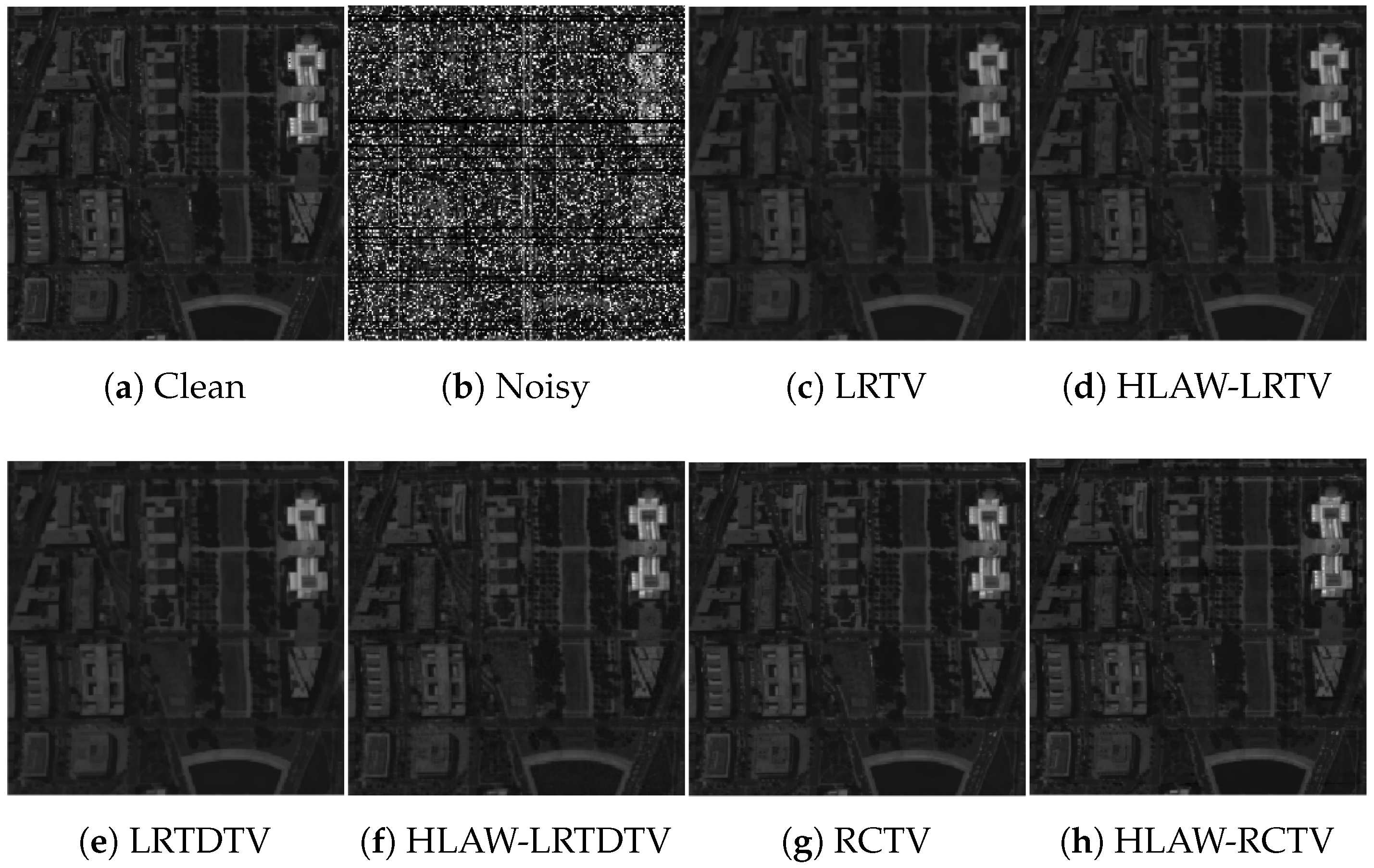
Visual Comparison: Figure 3 and Figure 4 illustrate the denoising performance of all competing algorithms on the 25th band of the PaviaC and WDC datasets. The noisy observations (b) are severely degraded by impulse noise, vertical stripes, and deadlines, causing most scene details to be overwhelmed. Deep-learning-based methods can remove noise effectively, but they suffer from heavy over-smoothing. Traditional low-rank models such as TNN, LRTF-DFR, and FastHyDe suppress part of the impulse noise yet leave conspicuous stripe residuals. NGmeet and LRTV further attenuate the stripes but suffer from heavy over-smoothing. The texture in PaviaC and the architectural details in WDC become blurred. LRTDTV, TCTV, E3DTV, and HNN successfully remove structured noise but introduce blocky artifacts. RCTV and ETPTV preserve geometric structures, though isolated impulse dots remain visible. The proposed HLAWTV almost completely eliminates impulse and stripe/deadlines corruption while retaining sharp boundaries. These observations substantiate the effectiveness and robustness of the HLSM prior combined with our adaptive weighting.

Table 2. Comparison of HSI denoising methods in terms of modeling properties and noise assumptions.

Method	Deep Learning Method	Low-Rank Modeling			Local Continuity		Non-Local Similarity	Gradient Distribution
		Spatial	Spectral	Both	Spatial	Spectral
QRNN3D	✓							-
ILRNet	✓							-
TNN				✓				-
LRTF-DFR				✓	✓	✓		Laplacian
FastHyDe			✓				✓	-
NGmeet			✓				✓	-
LRTV			✓		✓			Laplacian
LRTDTV				✓	✓	✓		Laplacian
TCTV			✓	✓	✓	✓		Laplacian
E3DTV					✓	✓		Laplacian
RCTV			✓		✓			Laplacian
ETPTV				✓	✓	✓		Laplacian
HNN				✓				-
HLAWTV (Ours)				✓	✓	✓		Hyper-Laplacian

Table 2. Comparison of HSI denoising methods in terms of modeling properties and noise assumptions.

Method	Deep Learning Method	Low-Rank Modeling			Local Continuity		Non-Local Similarity	Gradient Distribution
		Spatial	Spectral	Both	Spatial	Spectral
QRNN3D	✓							-
ILRNet	✓							-
TNN				✓				-
LRTF-DFR				✓	✓	✓		Laplacian
FastHyDe			✓				✓	-
NGmeet			✓				✓	-
LRTV			✓		✓			Laplacian
LRTDTV				✓	✓	✓		Laplacian
TCTV			✓	✓	✓	✓		Laplacian
E3DTV					✓	✓		Laplacian
RCTV			✓		✓			Laplacian
ETPTV				✓	✓	✓		Laplacian
HNN				✓				-
HLAWTV (Ours)				✓	✓	✓		Hyper-Laplacian

4.2. Real Data Experiments

To validate the proposed method under practical conditions, we executed experiments on two real HSI datasets. One of the real dataset selected is the Urban dataset whose size is 307 × 307 × 210, the other is the Indian Pines dataset with a size of 145 × 145 × 220. Both datasets are severely polluted, thereby furnishing a stringent benchmark for performance evaluation.

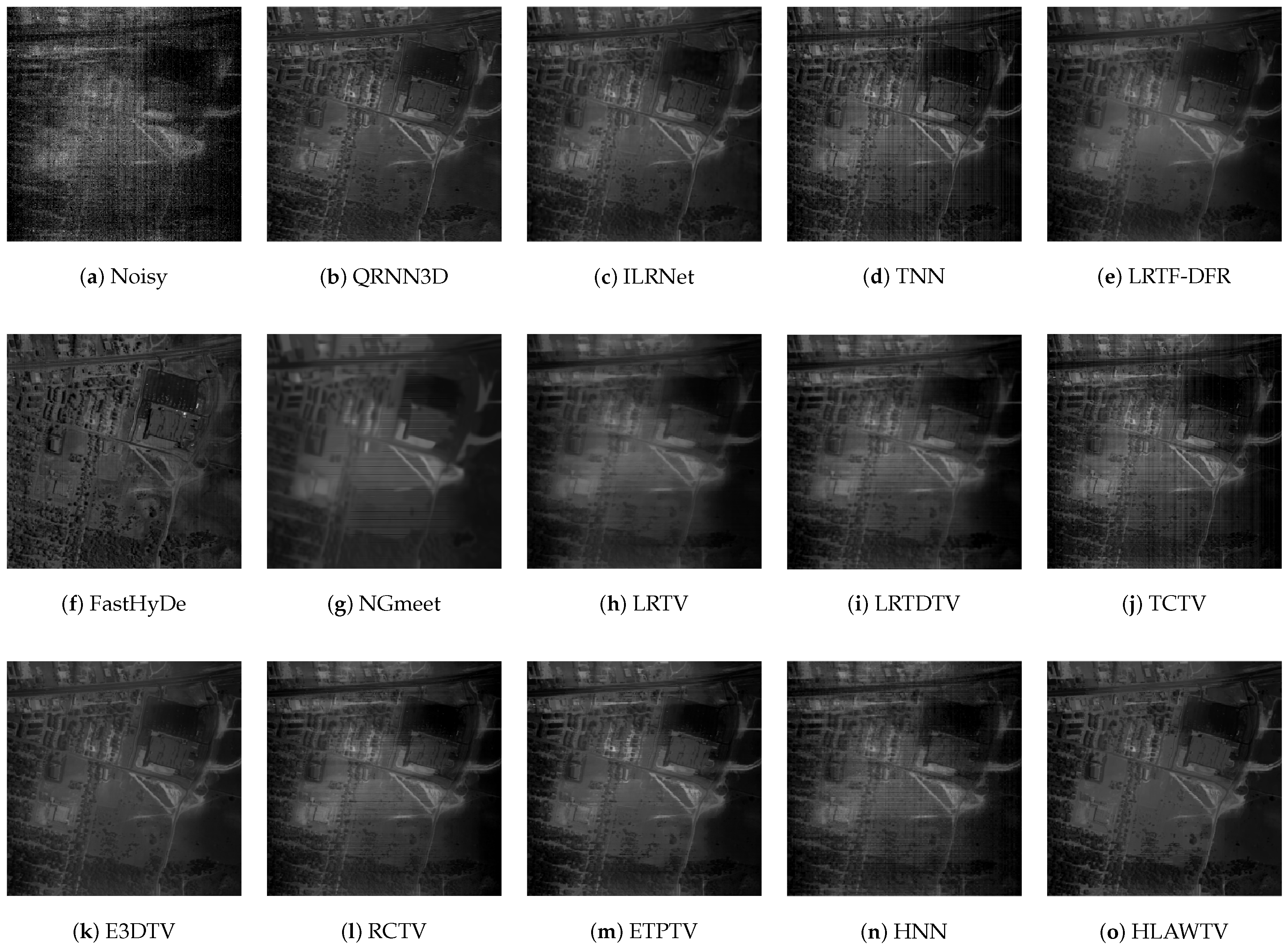
Figure 5 and Figure 6 show two representative bands of Urban. After denoising, methods such as QNNN3D, TNN, FastHyDe, LRTDTV, TCTV, RCTV, and HNN still exhibit obvious stripe noise. ILRNet, NGmeet, LRTV, and E3DTV produced noticeable over-smoothing. In contrast, HLAWTV simultaneously removed noise while preserving building edges and road textures.

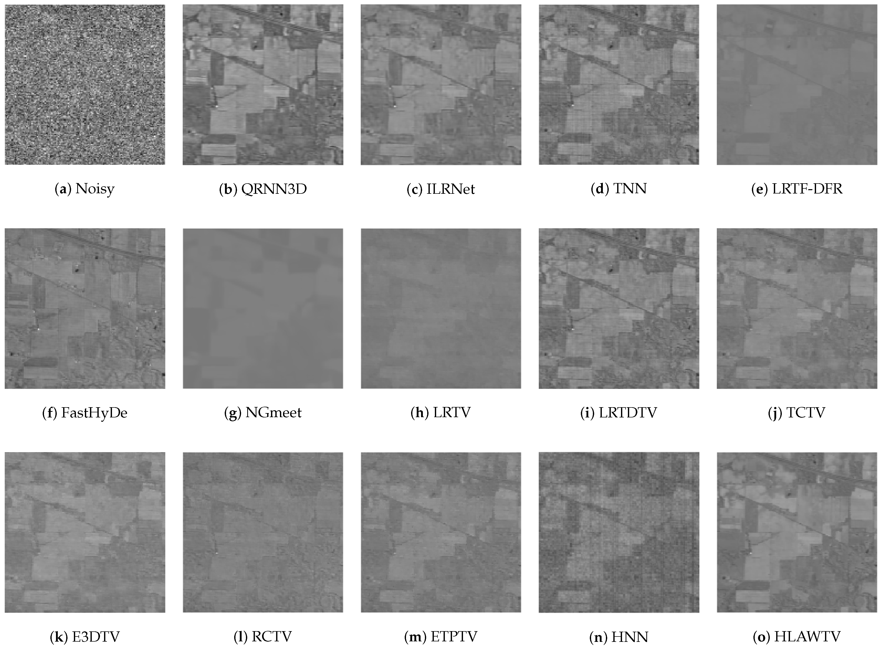
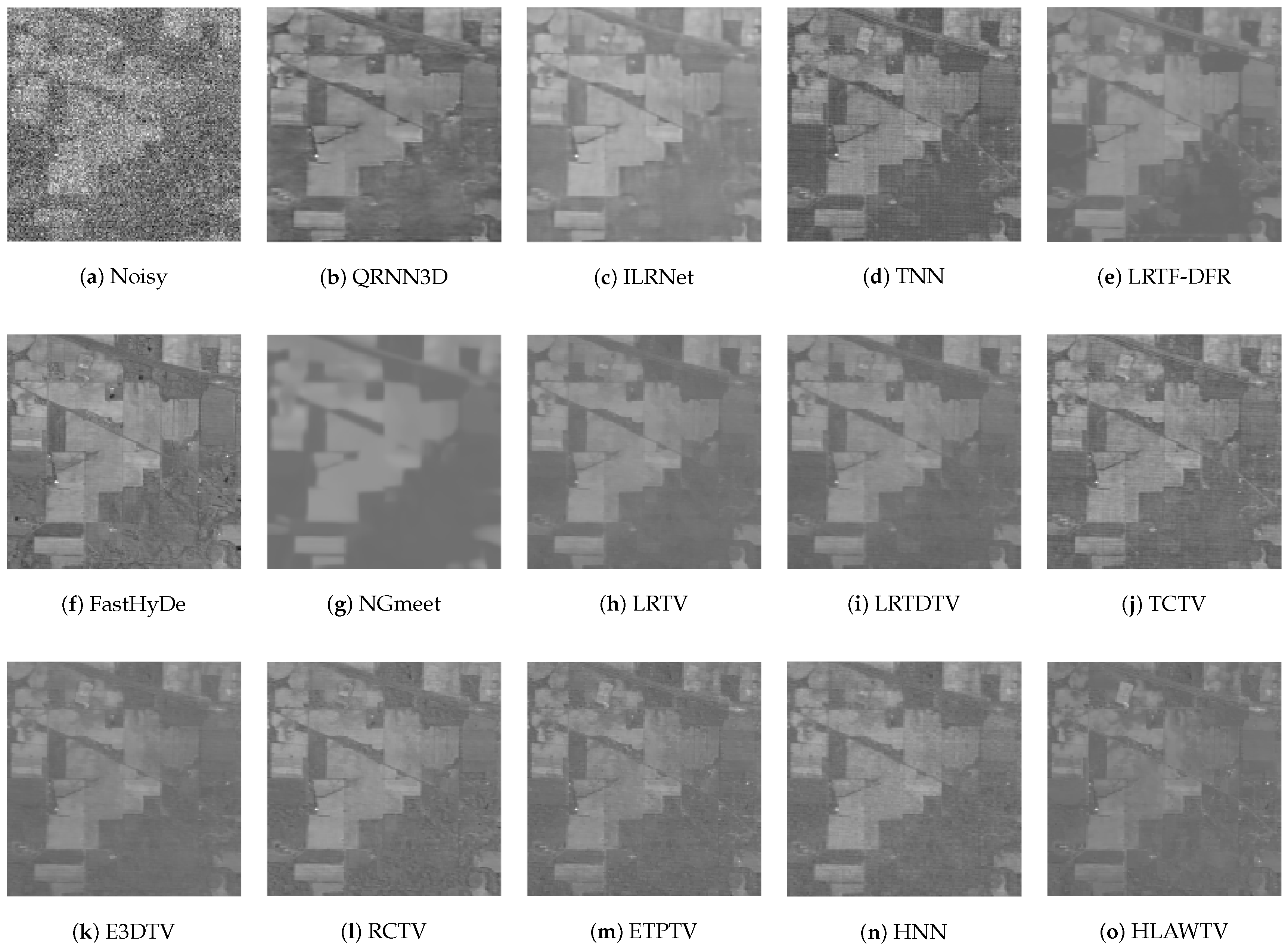
Figure 7 and Figure 8 show two bands from the Indian Pines dataset. The low-rankness based algorithm such as TNN, TCTV, and HNN mitigates Gaussian noise but is less effective against impulse noise. The conventional TV-based model performs better in removing impulse noise but blurs the farmland boundaries. HLAWTV effectively removes noise while maintaining clear texture.

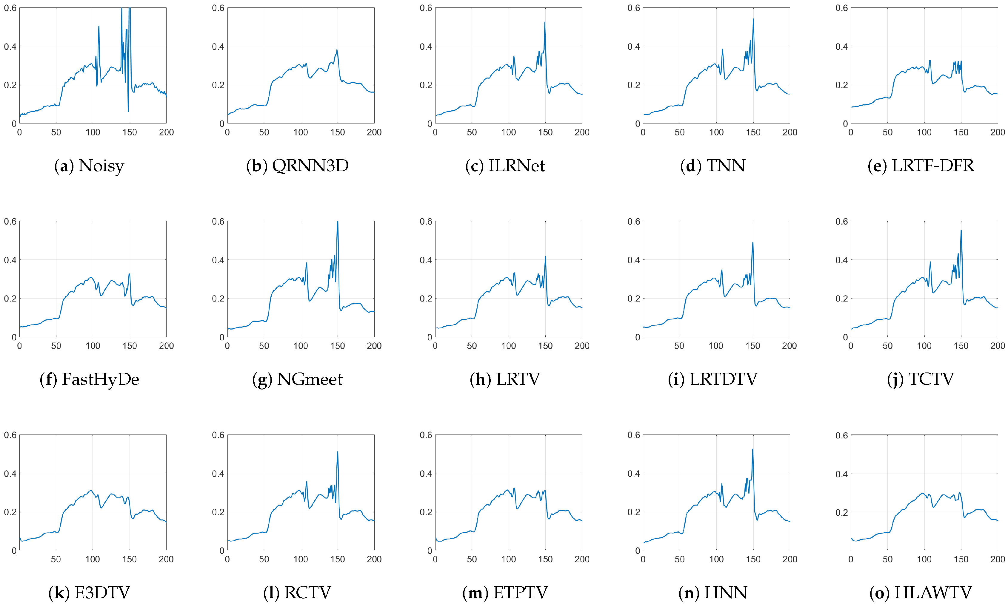
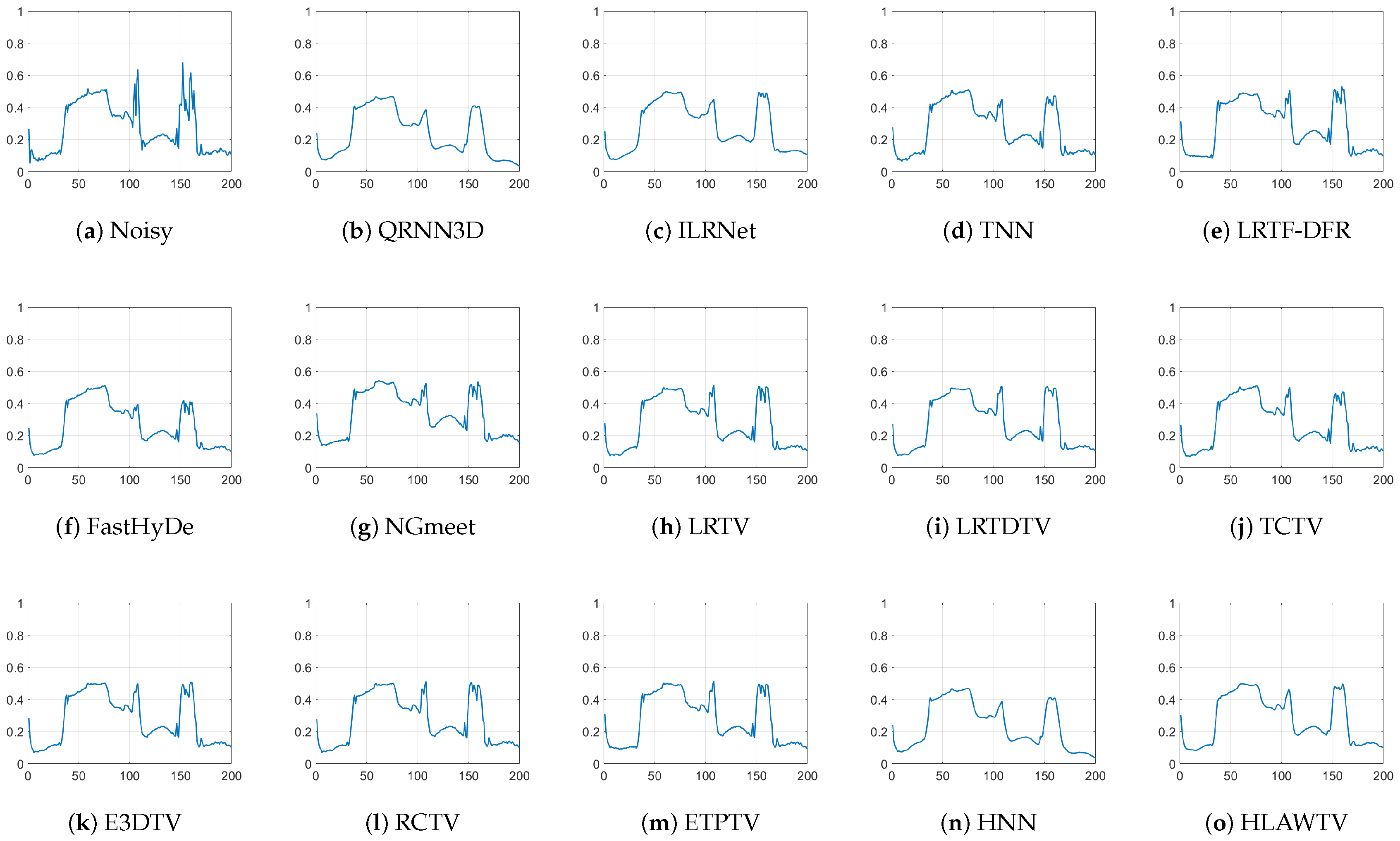
Figure 9 and Figure 10 plot the spectral features of the Urban pixel at (185, 132) and the Indian Pines pixel at (125,20). After ILRNet, TNN, NGmeet, LRTDTV, TCTV, RCTV, and HNN denoising, the strong spikes in the original spectral are partially suppressed. However, there are still noticeable fluctuations in several noisy bands, which implies that there is still residual noise interference. In contrast, the curves produced by the other methods are much smoother after denoising, indicating that the noise is well suppressed on all the bands.

To evaluate the denoising performance of various methods on real-noise datasets, we employ the Blind/Unreferenced Image Space Quality Evaluator (BRISQUE) [45] as the unreferenced metric to assess the results of different methods on the Urban and Indian Pines datasets. BRISQUE is a perceptual quality assessment metric that evaluates image quality based on the statistical characteristics of natural scenes, requiring no real reference images for evaluation. A lower BRISQUE score indicates higher image quality. The results are presented in Table 5.

Table 3. Quantitative indices of the PaviaC dataset with different methods under different cases.

Index	Noisy	QRNN3D	ILRNet	TNN	LRTF-DFR	FastHyDe	NGmeet	LRTV	LRTDTV	TCTV	E3DTV	RCTV	ETPTV	HNN	HLAWTV
Case 1: i.i.d. Gaussian Noise ($\sigma$ = 0.1)
MPSNR	20.592	31.085	34.474	25.381	34.345	34.532	24.513	30.383	32.881	30.046	33.700	34.161	34.411	32.322	34.892
MSSIM	0.416	0.913	0.928	0.628	0.926	0.925	0.489	0.814	0.884	0.818	0.909	0.918	0.924	0.932	0.937
MSAM	0.478	0.115	0.083	0.313	0.079	0.098	0.125	0.101	0.099	0.197	0.091	0.108	0.098	0.108	0.077
Time	0.000	0.155	1.494	50.793	13.338	0.197	23.126	8.913	26.564	1345.642	9.541	2.850	46.544	28.024	40.991
Case 2: non-i.i.d. Gaussian Noise (SNR ∈ [1, 15] dB)
MPSNR	27.494	33.246	39.197	31.966	38.270	42.050	25.067	34.101	36.090	36.089	36.176	38.644	39.787	36.932	39.997
MSSIM	0.712	0.948	0.940	0.866	0.967	0.984	0.533	0.915	0.945	0.942	0.951	0.963	0.973	0.977	0.974
MSAM	0.319	0.107	0.065	0.180	0.066	0.052	0.119	0.095	0.081	0.116	0.073	0.089	0.066	0.071	0.069
Time	0.000	0.271	1.893	50.020	13.118	0.188	22.637	8.675	26.502	1435.799	14.595	4.676	236.784	29.841	160.112
Case 3: Mixture of Gaussian and Impulse Noise
MPSNR	11.286	29.526	29.582	21.966	30.781	21.786	19.847	28.092	30.620	27.330	30.796	30.845	32.249	30.759	33.531
MSSIM	0.093	0.891	0.852	0.446	0.856	0.700	0.300	0.715	0.817	0.720	0.846	0.821	0.887	0.805	0.890
MSAM	0.788	0.113	0.130	0.406	0.106	0.151	0.163	0.133	0.120	0.239	0.107	0.177	0.113	0.117	0.103
Time	0.000	0.393	1.971	52.623	14.164	0.197	23.290	25.309	70.988	1508.890	13.481	4.532	228.653	30.250	153.020
Case 4: Mixed Impulse Noise + Stripes + Deadlines (Impulse Ratio 20%)
MPSNR	11.492	29.397	29.392	38.970	33.944	23.166	20.798	35.587	36.822	41.094	41.600	43.634	49.014	42.903	49.884
MSSIM	0.113	0.887	0.846	0.926	0.948	0.751	0.360	0.951	0.958	0.937	0.988	0.985	0.996	0.996	0.996
MSAM	0.799	0.117	0.134	0.206	0.078	0.144	0.156	0.092	0.083	0.200	0.045	0.051	0.034	0.043	0.033
Time	0.000	0.317	1.53	185.985	23.641	0.390	60.302	27.270	158.261	2348.431	9.611	2.811	46.316	27.931	42.589
Case 5: Mixed Impulse Noise + Stripes + Deadlines (Impulse Ratio 50%)
MPSNR	7.564	23.417	24.203	24.490	25.422	15.763	15.170	29.918	33.150	36.340	34.378	35.530	37.937	36.500	43.255
MSSIM	0.027	0.709	0.593	0.603	0.811	0.401	0.122	0.854	0.921	0.933	0.951	0.932	0.976	0.985	0.986
MSAM	0.859	0.158	0.170	0.342	0.113	0.203	0.204	0.147	0.110	0.172	0.074	0.109	0.054	0.065	0.054
Time	0.000	0.378	1.569	52.503	13.587	0.185	23.167	8.553	26.311	1146.588	9.176	2.690	45.512	40.109	45.334
Case 6: Mixed Gaussian + Impulse + Stripes + Deadlines
MPSNR	11.245	28.420	28.727	21.386	30.205	21.846	19.796	27.659	30.278	25.822	30.614	30.453	32.081	31.149	32.389
MSSIM	0.091	0.871	0.825	0.422	0.847	0.692	0.282	0.700	0.810	0.669	0.841	0.810	0.884	0.879	0.888
MSAM	0.789	0.122	0.142	0.431	0.119	0.158	0.168	0.157	0.133	0.292	0.111	0.203	0.117	0.129	0.109
Time	0.000	0.281	1.559	49.781	13.102	0.190	23.073	8.782	25.923	1178.679	9.476	2.652	46.392	94.718	40.634

Table 3. Quantitative indices of the PaviaC dataset with different methods under different cases.

Index	Noisy	QRNN3D	ILRNet	TNN	LRTF-DFR	FastHyDe	NGmeet	LRTV	LRTDTV	TCTV	E3DTV	RCTV	ETPTV	HNN	HLAWTV
Case 1: i.i.d. Gaussian Noise ($\sigma$ = 0.1)
MPSNR	20.592	31.085	34.474	25.381	34.345	34.532	24.513	30.383	32.881	30.046	33.700	34.161	34.411	32.322	34.892
MSSIM	0.416	0.913	0.928	0.628	0.926	0.925	0.489	0.814	0.884	0.818	0.909	0.918	0.924	0.932	0.937
MSAM	0.478	0.115	0.083	0.313	0.079	0.098	0.125	0.101	0.099	0.197	0.091	0.108	0.098	0.108	0.077
Time	0.000	0.155	1.494	50.793	13.338	0.197	23.126	8.913	26.564	1345.642	9.541	2.850	46.544	28.024	40.991
Case 2: non-i.i.d. Gaussian Noise (SNR ∈ [1, 15] dB)
MPSNR	27.494	33.246	39.197	31.966	38.270	42.050	25.067	34.101	36.090	36.089	36.176	38.644	39.787	36.932	39.997
MSSIM	0.712	0.948	0.940	0.866	0.967	0.984	0.533	0.915	0.945	0.942	0.951	0.963	0.973	0.977	0.974
MSAM	0.319	0.107	0.065	0.180	0.066	0.052	0.119	0.095	0.081	0.116	0.073	0.089	0.066	0.071	0.069
Time	0.000	0.271	1.893	50.020	13.118	0.188	22.637	8.675	26.502	1435.799	14.595	4.676	236.784	29.841	160.112
Case 3: Mixture of Gaussian and Impulse Noise
MPSNR	11.286	29.526	29.582	21.966	30.781	21.786	19.847	28.092	30.620	27.330	30.796	30.845	32.249	30.759	33.531
MSSIM	0.093	0.891	0.852	0.446	0.856	0.700	0.300	0.715	0.817	0.720	0.846	0.821	0.887	0.805	0.890
MSAM	0.788	0.113	0.130	0.406	0.106	0.151	0.163	0.133	0.120	0.239	0.107	0.177	0.113	0.117	0.103
Time	0.000	0.393	1.971	52.623	14.164	0.197	23.290	25.309	70.988	1508.890	13.481	4.532	228.653	30.250	153.020
Case 4: Mixed Impulse Noise + Stripes + Deadlines (Impulse Ratio 20%)
MPSNR	11.492	29.397	29.392	38.970	33.944	23.166	20.798	35.587	36.822	41.094	41.600	43.634	49.014	42.903	49.884
MSSIM	0.113	0.887	0.846	0.926	0.948	0.751	0.360	0.951	0.958	0.937	0.988	0.985	0.996	0.996	0.996
MSAM	0.799	0.117	0.134	0.206	0.078	0.144	0.156	0.092	0.083	0.200	0.045	0.051	0.034	0.043	0.033
Time	0.000	0.317	1.53	185.985	23.641	0.390	60.302	27.270	158.261	2348.431	9.611	2.811	46.316	27.931	42.589
Case 5: Mixed Impulse Noise + Stripes + Deadlines (Impulse Ratio 50%)
MPSNR	7.564	23.417	24.203	24.490	25.422	15.763	15.170	29.918	33.150	36.340	34.378	35.530	37.937	36.500	43.255
MSSIM	0.027	0.709	0.593	0.603	0.811	0.401	0.122	0.854	0.921	0.933	0.951	0.932	0.976	0.985	0.986
MSAM	0.859	0.158	0.170	0.342	0.113	0.203	0.204	0.147	0.110	0.172	0.074	0.109	0.054	0.065	0.054
Time	0.000	0.378	1.569	52.503	13.587	0.185	23.167	8.553	26.311	1146.588	9.176	2.690	45.512	40.109	45.334
Case 6: Mixed Gaussian + Impulse + Stripes + Deadlines
MPSNR	11.245	28.420	28.727	21.386	30.205	21.846	19.796	27.659	30.278	25.822	30.614	30.453	32.081	31.149	32.389
MSSIM	0.091	0.871	0.825	0.422	0.847	0.692	0.282	0.700	0.810	0.669	0.841	0.810	0.884	0.879	0.888
MSAM	0.789	0.122	0.142	0.431	0.119	0.158	0.168	0.157	0.133	0.292	0.111	0.203	0.117	0.129	0.109
Time	0.000	0.281	1.559	49.781	13.102	0.190	23.073	8.782	25.923	1178.679	9.476	2.652	46.392	94.718	40.634

Table 4. Quantitative indices of the WDC dataset with different methods under different cases.

Index	Noisy	QRNN3D	ILRNet	TNN	LRTF-DFR	FastHyDe	NGmeet	LRTV	LRTDTV	TCTV	E3DTV	RCTV	ETPTV	HNN	HLAWETV
Case 1: i.i.d. Gaussian Noise ($\sigma$ = 0.1)
MPSNR	20.713	30.260	34.145	25.296	35.137	35.708	35.681	30.235	32.508	29.570	32.947	35.228	35.587	33.536	35.874
MSSIM	0.407	0.877	0.933	0.615	0.953	0.956	0.955	0.837	0.904	0.807	0.922	0.950	0.956	0.933	0.957
MSAM	0.448	0.152	0.097	0.289	0.084	0.081	0.078	0.093	0.085	0.176	0.097	0.075	0.079	0.089	0.070
Time	0.000	0.727	3.27	592.092	78.912	0.701	105.312	117.485	1318.765	1303.256	53.931	13.624	1204.346	192.072	762.212
Case 2: non-i.i.d. Gaussian Noise (SNR ∈ [1, 15] dB)
MPSNR	28.366	31.838	38.018	32.462	37.408	42.157	34.787	33.327	34.507	35.615	35.817	38.326	39.323	37.980	39.977
MSSIM	0.739	0.907	0.968	0.888	0.973	0.988	0.946	0.915	0.940	0.949	0.958	0.976	0.982	0.979	0.984
MSAM	0.305	0.131	0.073	0.140	0.062	0.047	0.085	0.081	0.070	0.093	0.075	0.057	0.048	0.057	0.050
Time	0.000	0.837	3.741	207.009	50.741	0.367	43.734	54.412	254.309	1246.466	58.075	14.880	1267.650	214.052	829.846
Case 3: Mixture of Gaussian and Impulse Noise
MPSNR	11.425	28.677	30.002	23.137	33.716	22.258	19.693	28.954	31.447	27.914	31.331	33.607	34.015	32.005	34.230
MSSIM	0.113	0.860	0.856	0.508	0.937	0.779	0.462	0.796	0.880	0.746	0.891	0.928	0.939	0.906	0.940
MSAM	0.792	0.175	0.132	0.350	0.099	0.220	0.273	0.109	0.098	0.207	0.116	0.097	0.093	0.110	0.087
Time	0.000	0.926	3.84	387.397	54.884	0.371	39.023	47.733	100.479	645.359	58.416	12.720	365.138	91.146	258.205
Case 4: Mixed Impulse Noise + Stripes + Deadlines (Impulse Ratio $20\%$)
MPSNR	11.385	28.521	29.795	34.978	35.197	22.935	20.019	34.553	34.717	36.545	38.742	42.170	43.950	43.840	44.913
MSSIM	0.122	0.857	0.852	0.923	0.969	0.795	0.468	0.949	0.946	0.930	0.984	0.992	0.995	0.995	0.996
MSAM	0.804	0.179	0.136	0.175	0.064	0.209	0.270	0.064	0.065	0.170	0.042	0.028	0.027	0.019	0.018
Time	0.000	0.836	3.485	319.254	92.515	0.749	131.510	136.032	1168.649	951.130	65.150	16.020	870.936	85.302	274.423
Case 5: Mixed Impulse Noise + Stripes + Deadlines (Impulse Ratio $30\%$)
MPSNR	9.659	27.126	28.538	33.323	32.859	19.720	17.881	32.936	34.343	35.744	37.420	40.843	43.460	43.710	44.770
MSSIM	0.075	0.827	0.813	0.914	0.957	0.702	0.418	0.928	0.941	0.929	0.979	0.989	0.994	0.994	0.995
MSAM	0.851	0.193	0.151	0.176	0.077	0.262	0.302	0.084	0.069	0.167	0.050	0.030	0.028	0.020	0.020
Time	0.000	0.787	3.543	765.559	94.188	0.383	41.364	52.584	116.259	847.853	65.440	12.865	681.155	83.519	308.118
Case 6: Mixed Gaussian + Impulse + Stripes + Deadlines
MPSNR	11.214	28.171	29.370	22.136	32.377	21.828	21.425	28.492	30.995	26.562	30.574	32.578	33.488	29.224	33.809
MSSIM	0.104	0.851	0.842	0.464	0.921	0.761	0.650	0.781	0.870	0.704	0.871	0.911	0.935	0.837	0.937
MSAM	0.800	0.184	0.145	0.389	0.119	0.231	0.254	0.134	0.110	0.249	0.128	0.115	0.102	0.162	0.097
Time	0.000	0.844	3.548	636.327	168.988	0.367	39.662	48.769	102.941	933.142	55.822	14.374	533.271	89.439	238.935

Table 4. Quantitative indices of the WDC dataset with different methods under different cases.

Index	Noisy	QRNN3D	ILRNet	TNN	LRTF-DFR	FastHyDe	NGmeet	LRTV	LRTDTV	TCTV	E3DTV	RCTV	ETPTV	HNN	HLAWETV
Case 1: i.i.d. Gaussian Noise ($\sigma$ = 0.1)
MPSNR	20.713	30.260	34.145	25.296	35.137	35.708	35.681	30.235	32.508	29.570	32.947	35.228	35.587	33.536	35.874
MSSIM	0.407	0.877	0.933	0.615	0.953	0.956	0.955	0.837	0.904	0.807	0.922	0.950	0.956	0.933	0.957
MSAM	0.448	0.152	0.097	0.289	0.084	0.081	0.078	0.093	0.085	0.176	0.097	0.075	0.079	0.089	0.070
Time	0.000	0.727	3.27	592.092	78.912	0.701	105.312	117.485	1318.765	1303.256	53.931	13.624	1204.346	192.072	762.212
Case 2: non-i.i.d. Gaussian Noise (SNR ∈ [1, 15] dB)
MPSNR	28.366	31.838	38.018	32.462	37.408	42.157	34.787	33.327	34.507	35.615	35.817	38.326	39.323	37.980	39.977
MSSIM	0.739	0.907	0.968	0.888	0.973	0.988	0.946	0.915	0.940	0.949	0.958	0.976	0.982	0.979	0.984
MSAM	0.305	0.131	0.073	0.140	0.062	0.047	0.085	0.081	0.070	0.093	0.075	0.057	0.048	0.057	0.050
Time	0.000	0.837	3.741	207.009	50.741	0.367	43.734	54.412	254.309	1246.466	58.075	14.880	1267.650	214.052	829.846
Case 3: Mixture of Gaussian and Impulse Noise
MPSNR	11.425	28.677	30.002	23.137	33.716	22.258	19.693	28.954	31.447	27.914	31.331	33.607	34.015	32.005	34.230
MSSIM	0.113	0.860	0.856	0.508	0.937	0.779	0.462	0.796	0.880	0.746	0.891	0.928	0.939	0.906	0.940
MSAM	0.792	0.175	0.132	0.350	0.099	0.220	0.273	0.109	0.098	0.207	0.116	0.097	0.093	0.110	0.087
Time	0.000	0.926	3.84	387.397	54.884	0.371	39.023	47.733	100.479	645.359	58.416	12.720	365.138	91.146	258.205
Case 4: Mixed Impulse Noise + Stripes + Deadlines (Impulse Ratio $20\%$)
MPSNR	11.385	28.521	29.795	34.978	35.197	22.935	20.019	34.553	34.717	36.545	38.742	42.170	43.950	43.840	44.913
MSSIM	0.122	0.857	0.852	0.923	0.969	0.795	0.468	0.949	0.946	0.930	0.984	0.992	0.995	0.995	0.996
MSAM	0.804	0.179	0.136	0.175	0.064	0.209	0.270	0.064	0.065	0.170	0.042	0.028	0.027	0.019	0.018
Time	0.000	0.836	3.485	319.254	92.515	0.749	131.510	136.032	1168.649	951.130	65.150	16.020	870.936	85.302	274.423
Case 5: Mixed Impulse Noise + Stripes + Deadlines (Impulse Ratio $30\%$)
MPSNR	9.659	27.126	28.538	33.323	32.859	19.720	17.881	32.936	34.343	35.744	37.420	40.843	43.460	43.710	44.770
MSSIM	0.075	0.827	0.813	0.914	0.957	0.702	0.418	0.928	0.941	0.929	0.979	0.989	0.994	0.994	0.995
MSAM	0.851	0.193	0.151	0.176	0.077	0.262	0.302	0.084	0.069	0.167	0.050	0.030	0.028	0.020	0.020
Time	0.000	0.787	3.543	765.559	94.188	0.383	41.364	52.584	116.259	847.853	65.440	12.865	681.155	83.519	308.118
Case 6: Mixed Gaussian + Impulse + Stripes + Deadlines
MPSNR	11.214	28.171	29.370	22.136	32.377	21.828	21.425	28.492	30.995	26.562	30.574	32.578	33.488	29.224	33.809
MSSIM	0.104	0.851	0.842	0.464	0.921	0.761	0.650	0.781	0.870	0.704	0.871	0.911	0.935	0.837	0.937
MSAM	0.800	0.184	0.145	0.389	0.119	0.231	0.254	0.134	0.110	0.249	0.128	0.115	0.102	0.162	0.097
Time	0.000	0.844	3.548	636.327	168.988	0.367	39.662	48.769	102.941	933.142	55.822	14.374	533.271	89.439	238.935

Table 5. Blind/Referenceless Image Spatial Quality Evaluator (BRISQUE) comparison on the real data.

Index	Noisy	QRNN3D	ILRNet	TNN	LRTF-DFR	FastHyDe	NGmeet	LRTV	LRTDTV	TCTV	E3DTV	RCTV	ETPTV	HNN	HLAWTV
Urban	72.50	39.42	36.95	47.97	31.79	34.98	38.43	35.81	55.24	48.63	36.71	36.85	36.97	50.46	28.51
Indian Pines	93.57	31.72	25.12	27.75	34.74	45.96	61.85	27.71	28.96	64.02	24.76	35.88	35.39	57.97	23.49

Table 5. Blind/Referenceless Image Spatial Quality Evaluator (BRISQUE) comparison on the real data.

Index	Noisy	QRNN3D	ILRNet	TNN	LRTF-DFR	FastHyDe	NGmeet	LRTV	LRTDTV	TCTV	E3DTV	RCTV	ETPTV	HNN	HLAWTV
Urban	72.50	39.42	36.95	47.97	31.79	34.98	38.43	35.81	55.24	48.63	36.71	36.85	36.97	50.46	28.51
Indian Pines	93.57	31.72	25.12	27.75	34.74	45.96	61.85	27.71	28.96	64.02	24.76	35.88	35.39	57.97	23.49

5. Discussion

5.1. Transferring to Other TV Regularizers

In this section, we investigate the portability of the proposed HLAWTV framework by integrating it into several TV-based regularizers. Therefore, three representative baselines with distinct TV formulations are selected as follows: LRTV applied 2-D TV to each band individually. LRTDTV considered pixel-variation distributions along the three tensor modes and assigned mode-specific weights to the corresponding gradient maps. RCTV adopted 2-D TV on representative coefficients of HSIs. For each baseline, we replace its original TV term with the HLAWTV regularization to obtain HLAW-LRTV, HLAW-LRTDTV, and HLAW-RCTV. The solver only needs to make local modifications to the TV minimization subproblem, while the overall optimization framework remains unchanged.

We conducted comparison experiments on the WDC dataset with the same noise settings as the synthetic data experiments, and the quantitative and visual results are shown in

Table 6. Performance comparison of all competing methods on the WDC dataset.

Case	Index	Noisy HSI	LRTV	HLAW-LRTV	LRTDTV	HLAW-LRTDTV	RCTV	HLAW-RCTV
Case 1	MPSNR	20.713	30.235	32.419	32.508	33.984	35.228	35.982
	MSSIM	0.407	0.837	0.894	0.904	0.924	0.950	0.954
	SAM	0.448	0.093	0.080	0.085	0.070	0.070	0.068
	Time (s)	0.000	117.485	53.616	1318.765	120.483	13.624	11.541
Case 2	MPSNR	28.366	33.327	35.967	34.507	35.514	38.326	39.297
	MSSIM	0.739	0.915	0.952	0.940	0.949	0.976	0.977
	SAM	0.305	0.081	0.071	0.070	0.064	0.057	0.052
	Time (s)	0.000	54.412	199.817	254.309	127.898	14.880	19.052
Case 3	MPSNR	11.425	28.954	30.981	31.447	33.040	33.607	34.043
	MSSIM	0.113	0.796	0.863	0.880	0.908	0.928	0.929
	SAM	0.792	0.109	0.097	0.098	0.085	0.087	0.086
	Time (s)	0.000	47.733	199.955	100.479	837.385	12.720	11.162
Case 4	MPSNR	11.385	34.553	38.156	34.717	35.495	42.170	44.246
	MSSIM	0.122	0.949	0.976	0.946	0.950	0.992	0.995
	SAM	0.804	0.064	0.057	0.065	0.060	0.028	0.025
	Time (s)	0.000	136.032	54.355	1168.649	144.298	16.020	13.809
Case 5	MPSNR	9.659	32.936	36.625	34.343	35.396	40.843	43.245
	MSSIM	0.075	0.928	0.966	0.941	0.949	0.989	0.993
	SAM	0.851	0.084	0.066	0.069	0.060	0.030	0.026
	Time (s)	0.000	52.584	136.405	116.259	677.877	12.865	20.191
Case 6	MPSNR	11.214	28.492	30.395	30.995	32.177	32.578	33.050
	MSSIM	0.104	0.781	0.851	0.870	0.889	0.911	0.928
	SAM	0.800	0.134	0.125	0.110	0.109	0.115	0.107
	Time (s)	0.000	48.769	57.872	102.941	136.427	14.374	10.380

and Figure 11. It can be seen that the denoising performance is greatly improved after using our HLAWTV framework, which indicates that the weighting scheme can be finely ported to other TV regularizers and significantly improve the performance of the original model.

5.2. Ablation Study

To evaluate the effectiveness of each component in our proposed HLAWTV model, we perform a comprehensive ablation study on the WDC dataset under Case 5. Starting from the baseline LTV model, we progressively incorporate the following two key modules: adaptive weighting (AW) and HLSM. The results are shown in Table 7.

The LTV+AW model enables adaptive adjustment of the sparsity constraint between smooth and textured regions, thereby better preserving textures and edges in the image. However, due to the absence of global gradient sparsity modeling, its performance in terms of structural similarity and spectral accuracy remains suboptimal. In contrast, the LTV+HLSM model enhances global gradient sparsity by adjusting a heavy-tailed distribution on the gradients. Yet, it applies uniform penalties across the entire image without distinguishing between smooth and textured regions, leading to a lack of local adaptivity.

Although both AW and HLSM individually lead to slight decreases in SSIM and SAM compared to the baseline, their combination in the HLAWTV model results in the best overall performance across all three metrics (MPSNR, MSSIM, and MSAM). This clearly demonstrates the strong coupling between the following two components: adaptive weights enhance local sensitivity, while the Hyper-Laplacian prior ensures global denoising robustness.

Moreover, applying our proposed adaptive weighting design to the baseline LTV significantly reduces computation time. This confirms the effectiveness of leveraging the conjugacy between the Hyper-Laplacian and Gamma distributions to derive efficient, data-driven weight estimation. The resulting balance between computational efficiency and denoising quality highlights the practical value of our method in real-world applications.

Table 7. Ablation study results.

Method	MPSNR	MSSIM	MSAM	Time (s)
LTV	43.460	0.994	0.028	681
LTV+AW	43.901	0.983	0.032	232
LTV+HLSM	43.923	0.985	0.026	319
HLAWTV	44.770	0.995	0.020	308

Table 7. Ablation study results.

Method	MPSNR	MSSIM	MSAM	Time (s)
LTV	43.460	0.994	0.028	681
LTV+AW	43.901	0.983	0.032	232
LTV+HLSM	43.923	0.985	0.026	319
HLAWTV	44.770	0.995	0.020	308

5.3. Parameter Analysis

The robustness of the proposed HLAWTV model to its hyper-parameters $\lambda$ and rank $(r_1,r_2,r_3)$ is evaluated on the simulated data of Case 4. In this case, the denoising quality is monitored with MPSNR and MSSIM while a single parameter is varied and all others are fixed. Each experiment is repeated ten times to obtain statistically reliable curves.

First, we investigated the effect of the regularization parameter $\lambda$ on denoising performance. As shown in Figure 12a, when $\lambda$ is small, the HLAWTV regularization plays a minor role in the model, resulting in inadequate noise suppression and thus low MPSNR values with visible residual artifacts remaining in the denoised images. As $\lambda$ gradually increases, more noise is effectively eliminated, leading to a rapid improvement in MPSNR and optimal preservation of image structures at the peak value. However, further increasing $\lambda$ causes the regularization to become excessively strong, which in turn leads to over-smoothing and a loss of fine spatial details, causing the MPSNR to gradually decrease. Nevertheless, it is noteworthy that within a certain range of $\lambda$, the MPSNR remains consistently high, indicating that the model exhibits acceptable sensitivity to this parameter in practical applications. In summary, $\lambda$ controls the strength of HLAWTV regularization, and its optimal value can be chosen based on the smoothness of the image as follows: smoother images generally require a larger $\lambda$, while images with more texture or detail benefit from a smaller $\lambda$.

The factor rank in HLAWTV is specified by a triplet $(r_1,r_2,r_3)$, which controls the dimensionality of the low-rank subspace along the two spatial modes and the spectral mode. As shown in Figure 12b, varying these three ranks exhibits a clear pattern as follows: MPSNR increases rapidly as $r_1,r_2$, and $r_3$ grow from small values, reflecting the enhanced preservation of spatial and spectral structures. As $r1\ge 5$ and $r2\ge 5$ rise, the MPSNR plateaus and remains stable over a broad range of higher rank values, indicating that the model is robust to the choice of these parameters within this interval and does not easily overfit.

Overall, these parameter studies demonstrated the robustness of the proposed method and provided clear practical guidelines for selecting optimal parameter settings under various noise.

6. Conclusions

In this article, we proposed the Hyper-Laplacian Adaptive Weighted Total Variation model for hyperspectral image denoising. By integrating a Hyper-Laplacian Scale Mixture prior and leveraging the conjugacy between Gamma and Hyper-Laplacian distributions, our method efficiently computes adaptive weights that reflect the local sparsity and heavy-tailed characteristics of spatial-spectral gradients. The adaptive weighting, shared across all spectral bands at each pixel but varying spatially, enables precise noise suppression and detail preservation. Extensive experiments on both synthetic and real datasets demonstrated that HLAWTV consistently outperforms existing state-of-the-art methods. Furthermore, embedding our adaptive weighting mechanism into conventional total variation frameworks significantly enhances their effectiveness, confirming the broad applicability and robustness of our approach.