SATRNet: Self-Attention-Aided Deep Unfolding Tensor Representation Network for Robust Hyperspectral Anomaly Detection

Abstract

Hyperspectral anomaly detection (HAD) aims to separate subtle anomalies of a given hyperspectral image (HSI) from its background, which is a hot topic as well as a challenging inverse problem. Despite the significant success of the deep learning-based HAD methods, they are hard to interpret due to their black-box nature. Meanwhile, deep learning methods suffer from the identity mapping (IM) problem, referring to the network excessively focusing on the precise reconstruction of the background while neglecting the appropriate representation of anomalies. To this end, this paper proposes a self-attention-aided deep unfolding tensor representation network (SATRNet) for interpretable HAD by solving the tensor representation (TR)-based optimization model within the framework of deep networks. In particular, a Self-Attention Learning Module (SALM) was first designed to extract discriminative features of the input HSI. The HAD problem was then formulated as a tensor representation problem by exploring both the low-rankness of the background and the sparsity of the anomaly. A Weight Learning Module (WLM) exploring local details was also generated for precise background reconstruction. Finally, a deep network was built to solve the TR-based problem through unfolding and parameterizing the iterative optimization algorithm. The proposed SATRNet prevents the network from learning meaningless mappings, making the network interpretable to some extent while essentially solving the IM problem. The effectiveness of the proposed SATRNet is validated on 11 benchmark HSI datasets. Notably, the performance of SATRNet against adversarial attacks is also investigated in the experimentation, which is the first work exploring adversarial robustness in HAD to the best of our knowledge.

1. Introduction

Hyperspectral anomaly detection (HAD), which enables the identification of subtle, unknown materials within hyperspectral images (HSIs), represents a fundamental task in hyperspectral data analysis [1]. HAD typically operates in an unsupervised manner without requiring prior spectral knowledge of targets, aiming to detect objects whose spectral characteristics significantly differ from their background [2]. This unique capability renders HAD particularly valuable for various surveillance applications, where specific targets are unknown beforehand, including but not limited to the following: detecting camouflaged personnel in battlefield scenarios [3], identifying pesticide residues during food safety inspections [4], and locating tumors in medical imaging [5].

In the nascent stage of HAD development, statistical-based methods predominated in this field. These approaches, rooted in signal detection theory, were primarily employed for background characterization. The Reed–Xiaoli (RX) detector [6], derived from a binary hypothesis testing framework under a multivariate Gaussian distribution assumption, subsequently became the most widely adopted HAD method due to its algorithmic simplicity and computational efficiency. Its numerous variants rapidly proliferated, including local-RX (LRX) [7], which exclusively utilizes pixels from dual concentric sliding windows to maintain uncontaminated background sets, weighted-RX (WRX) [8], which strategically implements weighting schemes to enhance background representation and improve the detection performance of RX, and kernel-RX (KRX) [9], which projects original data into higher-dimensional feature spaces through nonlinear mapping to amplify separability between background and anomalies. Further methodological innovations introduced using the signal-to-noise ratio (SNR) as an alternative optimization criterion for detector design [10]. Notably, the formulation of a hyperspectral target detection (HTD) dual theory specifically for HAD applications marked the first comprehensive exploration of their inherent duality relationships.

However, statistical assumption-based approaches for HAD algorithm design encounter a fundamental limitation: the unknown probability density function in practical applications. This challenge has led to the widespread investigation and application of sparse coding (SC) [11,12] and matrix low-rank representation (MLRR) [13,14,15] techniques in HAD research. These methods rely on carefully designed regularization terms that employ various norms to capture essential data characteristics, particularly low-rankness and sparsity properties. SC-based HAD approaches utilize over-complete dictionaries with multiple atoms to represent test pixels through ${\mathsf{\ell }}_1$-norm optimization, as demonstrated in background joint SC [11] and archetypal analysis with structured SC [12]. At the matrix level, common optimization objectives incorporate the Frobenius norm, ${\mathsf{\ell }}_{2,1}$-norm, and nuclear norm to enforce desired structural properties. The low-rank and sparse representation (LRASR) framework [13] unifies these concepts by jointly modeling low-rank structures in coefficient matrices and sparse structures in residual matrices. By imposing nuclear norm constraints on the coefficient matrix, LRASR effectively captures the intrinsic HSI structure while isolating anomalies. Further developments, like graph and total variation regularized low-rank representation (GTVLRR) [14], augment the capabilities of LRASR through dual regularization terms that better preserve spatial structures. Recent advances include nonconvex-based HAD [15], where generalized shrinkage mapping achieves three objectives: approximating ${\mathsf{\ell }}_{2,0}$ penalties through group sparsity constraints, simulating ${\mathsf{\ell }}_0$ TV penalties via TV regularization, and enforcing low-rank properties with nuclear norm penalties. This integrated approach enables comprehensive spatial correlation modeling.

The intrinsic data structure of HSI is fundamentally tensor-based, while most existing methods convert the HSI data into matrix form. This will potentially compromise the inherent spatial characteristics of HSI. In contrast, tensor representation (TR) methods preserve spatial information completely, consequently achieving enhanced HAD performance. The TR algorithms focus on tensor rank minimization, where (unlike matrix rank) multiple definitions exist, including but not limited to the following: CANDECOMP/PARAFAC (CP) rank [16], Tucker rank [17], ring rank [18], average rank [19], and tubal rank [20]. A CP rank-based TR model [16] decomposes backgrounds via mode-3 products of abundance tensors and endmember matrices while preserving spatial-spectral integrity. By leveraging the inherent sparsity of core tensors generated through Tucker decomposition of gradient tensors, a specialized regularization term [17] is developed. This unified term simultaneously encodes both the low-rank and local smoothness constraints of background components, consequently improving HAD detection performance. The tensor ring decomposition (TRD) method [18] effectively exploits low-rank characteristics inherent in HSI background tensors. This approach decomposes a third-order background tensor through multilinear tensor products of three factor tensors, systematically uncovering low-rank features across different dimensionalities of the background tensor. A TR model [19] incorporates both low average rank and piecewise smooth constraints, employing the tensor nuclear norm (TNN) derived from tensor singular value decomposition (T-SVD) to induce low-rank properties on the background tensor. The tensor low-rank and sparse representation (TLRSR) framework [20] extends LRASR to the tensor domain, employing the weighted tensor nuclear norm (WTNN) as the convex relaxation for tensor tubal rank. This formulation enables computationally efficient Fourier-domain implementation while maintaining strong theoretical guarantees. The TLRSR further incorporates the ${\mathsf{\ell }}_{F,1}$ norm to enforce structured group sparsity constraints. As a tensor dictionary representation model, the spatial invariant tensor self-representation (SITSR) model [21] merges the unfolded matrices of two representative coefficients and constrains them in a low-dimensional subspace. This strategy fully preserves the multi-dimensional structure. Beyond convex formulations, some nonconvex TR methods [22,23,24] have been explored as alternatives to unbiased estimators. These nonconvex formulations can be replaced to promote sparsity, group sparsity, and low-rankness, which have shown obvious advantages in HAD.

More recently, the deep learning (DL) technique has achieved significant success in multiple real-world tasks [25,26,27,28]. This rapid development in DL also prompted numerous researchers to apply it to HAD, as evidenced by the growing body of work in this field [29,30,31,32,33,34,35]. The well-known deep learning method is the autonomous HAD (Auto-AD) network [29], which uses a fully convolutional autoencoder (AE) network to reconstruct the background and uses the reconstruction error as the anomaly score. Auto-AD applies an adaptive weighted loss function to further reduce the reconstruction of anomalies by lowering the weight of anomalous pixels during training. The robust graph autoencoder (RGAE) [30] incorporates a graph regularization term to preserve the spatial geometric structure during the reconstruction process. RGAE utilizes a superpixel segmentation-based graph regularization term instead of constructing a graph Laplacian matrix to reduce the computational complexity. In addition, the ${\mathsf{\ell }}_{2,1}$ norm is introduced into the loss function to improve the robustness to anomalies. The transformer-based AE framework (TAEF) [31] customizes the multilinear transformation decoder, which aims to improve the background learning capability of vanilla AE. In the preprocessing phase, TAEF uses a clustering-based method to suppress anomalies. The deep feature aggregation network (DFAN) [32] discovers the anomalies by enhancing the representation of various background patterns and calculating the Mahalanobis distance of the residual results. The gated transformer Network for HAD (GT-HAD) [33] is a dual-branch framework consisting of the anomaly-focused branch and the gated transformer block to accurately reconstruct the background while suppressing the anomalies. To further improve HAD performance, some studies have built deep networks based on the dual-window idea [34,35]. The spatial-spectral dual window mask transformer (S2DWMTrans) [34] makes full use of spatial-spectral information. Specifically, S2DWMTrans develops the local shallow feature extraction module to integrate adjacent spatial information, and the encoder block based on dual-window mask multihead self-attention further eliminates anomalies. Moreover, DirectNet [35] incorporates a sliding dual-window model to adaptively reconstruct the background, which increases the reconstruction error of anomalies.

Although the DL-based methods have become promising approaches in HAD, there are still some challenges. As mentioned in [36,37,38], the DL-based HAD methods widely suffer from the identity mapping (IM) problem, which refers to the phenomenon that the network reconstructs the whole HSI completely so that the anomalies are represented with imperceptible errors and, thus, are hard to detect. Moreover, the black-box nature of DL-based HAD methods makes them lack interpretability, which aggravates the IM issue to some extent. In fact, most of the existing DL-based methods, no matter how the architecture varies, learn meaningless mappings more or less due to the lack of interpretability and finally drive the network towards IM. On the contrary, traditional methods such as TR algorithms are fully interpretable and do not suffer from the IM problem, despite their limited generalization capability. Based on this observation, we naturally think of combining the TR methods with DL-based methods. Inspired by the deep unfolding technology, we propose a self-attention-aided deep unfolding tensor representation network called SATRNet for HAD. Specifically, SATRNet introduces Deep Unfolding Tensor Representation (DUTR), the architecture of which is designed by unfolding a customized TR algorithm. Due to the global modeling nature of DUTR, a Weight Learning Module (WLM) was developed to inject local details, enhancing the accuracy of background reconstruction. Moreover, a Self-Attention Learning Module (SALM) was introduced before DUTR to extract discriminative features, weakening the subsequent network’s ability to reconstruct the anomalies. In this way, the working principles of the key components in SATRNet are consistent with the iterative algorithms of TR models, which avoids the meaningless feature mappings of the black-box models, and the network is guided towards the explicit objective. The IM problem can be effectively alleviated and thus enhance HAD performance and generalization capability. The main contributions of this work can be summarized as follows:

• An interpretable network, the deep unfolding tensor representation network, is developed for HAD, solving the traditional TR model within a deep network. The combination of these two techniques integrates the interpretability of the TR model and the efficiency of the deep network for reliable anomaly detection. Moreover, a Weight Learning Module (WLM) is designed to learn local details to accurately reconstruct the background.
• A Self-Attention Learning Module (SALM) is introduced to extract discriminative features, which avoids reconstructing the anomalies during the background reconstruction process. This also helps to effectively alleviate the identity mapping (IM) problem.
• Apart from systematic evaluation against 11 HSI benchmark datasets, the adversarial attack experiment for HAD is performed in this work for the first time, indicating the adversarial robustness of the proposed SATRNet.

The rest of this paper is organized as follows. Notations, basic definitions, and related works are introduced in Section 2. Section 3 presents the proposed SATRNet model in detail. Comprehensive experimental results are given in Section 4. Discussions on the adversarial robustness of the proposed method are provided in Section 5. Finally, Section 6 concludes the paper.

2. Preliminaries

This section provides notations, basic definitions, and reviews of related works.

2.1. Notations and Basic Definitions

In this work, scalars, vectors, matrices, and tensors are represented by lowercase, bold lowercase, bold uppercase, and bold calligraphic uppercase letters, respectively, e.g., a, $\mathit{a}$, $\mathit{A}$, and $\mathcal{A}$. For a third-order tensor $\mathcal{A}\in {\mathbb{R}}^{n_1\times n_2\times n_3}$, ${\mathcal{A}}_{\left(i\right)}$ is the ith frontal slice of $\mathcal{A}$. In addition, $unfold\left(\mathcal{A}\right)$ converts $\mathcal{A}$ into a matrix with dimensions $n_1{n}_3\times n_2$, and $fold(·)$ is its inverse operator. The block circulant matrix $bcirc\left(\mathcal{A}\right)$ is defined as

$$\begin{array}{c}\hfill bcirc\left(\mathcal{A}\right)=\left[\begin{array}{cccc}{\mathcal{A}}_{\left(1\right)}& {\mathcal{A}}_{\left(n_3\right)}& \dots & {\mathcal{A}}_{\left(2\right)}\\ {\mathcal{A}}_{\left(2\right)}& {\mathcal{A}}_{\left(1\right)}& \dots & {\mathcal{A}}_{\left(3\right)}\\ ⋮& ⋮& \ddots & ⋮\\ {\mathcal{A}}_{\left(n_3\right)}& {\mathcal{A}}_{(n_3-1)}& \dots & {\mathcal{A}}_{\left(1\right)}\end{array}\right]\end{array}.$$

(1)

For unary operations, the ${\mathsf{\ell }}_1$-norm ${\parallel ·\parallel }_1$ and Frobenius norm ${\parallel ·\parallel }_F$ of $\mathcal{A}$ are defined as

$$\begin{array}{c}\hfill {\parallel \mathcal{A}\parallel }_1=\sum _{i_1=1}^{n_1}\sum _{i_2=1}^{n_2}\sum _{i_3=1}^{n_3}\left|{\mathcal{A}}_{i_1{i}_2{i}_3}\right|\end{array},$$

(2)

$$\begin{array}{c}\hfill {\parallel \mathcal{A}\parallel }_F=\sqrt{\sum _{i_1=1}^{n_1}\sum _{i_2=1}^{n_2}\sum _{i_3=1}^{n_3}{\left|{\mathcal{A}}_{i_1{i}_2{i}_3}\right|}^2}\end{array}.$$

(3)

For binary operations, the inner product $\langle ·,·\rangle$ of tensors $\mathcal{A},\mathcal{C}\in {\mathbb{R}}^{n_1\times n_2\times n_3}$ is defined as

$$\begin{array}{c}\hfill \langle \mathcal{A},\mathcal{C}\rangle =\sum _{i_1=1}^{n_1}\sum _{i_2=1}^{n_2}\sum _{i_3=1}^{n_3}{\mathcal{A}}_{i_1{i}_2{i}_3}{\mathcal{C}}_{i_1{i}_2{i}_3}\end{array}.$$

(4)

Furthermore, the tensor–tensor product (t-product) [39] of $\mathcal{A}\in {\mathbb{R}}^{n_1\times n_2\times n_3}$ and $\mathcal{C}\in {\mathbb{R}}^{n_2\times n_4\times n_3}$ is defined as

$$\begin{array}{c}\hfill \mathcal{A}\ast \mathcal{C}=fold(bcirc(\mathcal{A})·unfold(\mathcal{C}\left)\right)\end{array}.$$

(5)

2.2. Related Works

(1) Alternating direction method of multiplier (ADMM) [40]: The ADMM method has been proven to be effective in dealing with constrained optimization problems. This algorithm decomposes the original problem into several manageable subproblems by introducing auxiliary variables and is able to derive closed-form solutions for each subproblem, thereby significantly improving computational efficiency. The algorithmic structure of ADMM is naturally suitable for handling structured sparsity constraints in high-dimensional data, a characteristic that makes it particularly valuable in the field of remote sensing image analysis [41]. Specifically, in the HAD task, ADMM is one of the preferred tools for solving optimization problems involved in MLRR [15] and TR [20] approaches.

(2) Deep unfolding: Recently, the deep unfolding technique has made significant progress in fusion [42], super-resolution [43], pansharpening [44], and so on. The deep unfolding network is designed according to a model-based iterative algorithm by cascading basic units, where each basic unit corresponds to a single iteration of the algorithm, and multiple basic units are connected into a deep network. By combining the interpretability of the iterative algorithm with the data-driven learning ability of the deep network, deep unfolding benefits from the advantages of both methods, i.e., better interpretability and generalization. As stated in [45,46], deep unfolding usually can achieve better performance compared with model-driven versus data-driven methods.

In the field of HAD, deep unfolding technology has also been explored recently. The basic idea of these approaches is to correspond the operators of traditional models with the network structure and transform the regularization parameters into learnable deep network parameters. For example,  LRR-Net [46] is a kind of generalized deep unfolding network, in which the traditional MLRR model is unfolded into an unsupervised interpretable network. On this basis, by embedding sparsity, the LRR-Net framework also demonstrates certain scalability. LRSR-I2Net-TV [47] is also an unfolding network based on MLRR. Different from LRR-Net, LRSR-I2Net-TV introduces the TV regularization term in an effort to compensate for the spatial correlation ignored in the MLRR model. However, these methods still have obvious limitations. Firstly, they are matrix-based methods that only realize the mining of spectral information. Although LRSR-I2Net-TV introduces TV regularization, it only provides limited utilization of spatial information, but inevitably increases the computational burden. Secondly, these approaches usually rely on original image features, which may hinder the accurate separation of anomalies and their backgrounds due to spectral variation and noise pollution. Therefore, it is necessary to develop more advanced solutions for deep unfolding-based HAD.

(3) Self-attention mechanism: Self-attention mechanism, as the core of transformer, is outstanding in constructing global spatial dependencies. In HAD, residual self-attention-based autoencoder (RSAAE) [48] exploits self-attention mechanism to highlight the features with high attention weight values, i.e., background features. Meanwhile, a low-rank constraint loss function is designed to preserve the low-rank property of the background in the latent space. In [49], a self-attention suppression (SAS) module is developed to reduce the impact of anomalies. By combining the SAS module with a multi-scale feature extraction strategy, the network can better minimize Please check that intended meaning has been retained the essential data features, thus improving the effect of background reconstruction.

3. Methodology

For an input HSI tensor $\mathcal{M}\in {\mathbb{R}}^{h\times w\times c}$, where h, w, and c express the height, width, and bands, respectively, the proposed SATRNet finally outputs the corresponding anomaly map $\mathit{B}\in {\mathbb{R}}^{h\times w}$. Figure 1 shows a schematic of the proposed SATRNet. SATRNet primarily consists of two parts: Self-Attention Learning Module (SALM) and Deep Unfolding Tensor Representation (DUTR), which are introduced in Section 3.1 and Section 3.2, respectively.

3.1. SALM: Self-Attention Learning Module

The raw pixels of the input HSI usually contain redundant information and are easily disturbed by noise; therefore, the learned features are generally used in the literature [50,51,52]. However, due to the limited receptive field of standard convolutions, global contexts are usually not adequately modeled. While dilated convolutions, deeper networks, or equivalent strategies can expand the receptive field, they risk overfitting. The attention mechanism enables the model to dynamically focus on important parts, which has been proven to be a powerful tool for feature extraction [53]. Thus, before the deep unfolding process, we introduce a Self-Attention Learning Module (SALM) to capture the discriminative and representative feature of the input HSI.

As shown in Figure 2, SALM includes a self-attention layer and a feed-forward network (FFN) layer. The FFN consists of $1\times 1$ convolution, $3\times 3$ convolution, and leaky rectified linear unit layers, following the common practice in [54]. In the self-attention layer, given the input tensor $\mathcal{M}$, the output of this layer is ${\mathcal{M}}^{\ast }$. The $\mathit{Q},\mathit{K},\mathit{V}\in {\mathbb{R}}^{hw\times c}$ are obtained through feature projection and patch embedding. A kernel operation based on Mercer’s theorem [55] is employed to reconstruct $\mathit{Q}$ and $\mathit{K}$ for robust feature extraction. The kernel operation $\psi (·)$ is expressed as follows (taking $\mathit{Q}$ as an example):

$$\begin{array}{cc}\hfill \psi \left(\mathit{Q}\right)& =(1,{\displaystyle \frac{{(\mathit{Q}-\overline{\mathit{Q}})}^2}{{\sigma }^{\frac{1}{2}}}},{\displaystyle \frac{{(\mathit{Q}-\overline{\mathit{Q}})}^4}{{\sigma }^{\frac{1}{2}}}},\dots ,{\displaystyle \frac{{(\mathit{Q}-\overline{\mathit{Q}})}^{2i}}{{\sigma }^{\frac{1}{2}}}}).\hfill \end{array}$$

(6)

where $\overline{\mathit{Q}}$ represents the mean of $\mathit{Q}$, and $\sigma$ controls the scale of kernel operation $\psi (·)$. Furthermore, the computational efficiency is improved by changing the order of multiplication in self-attention, i.e., first multiplying $\mathit{K}$ and $\mathit{V}$. The formula for calculating the self-attention matrix SA is as follows:

$$\begin{array}{c}\hfill SA(\mathit{Q},\mathit{K},\mathit{V})=softmax\left({\displaystyle \frac{{\psi \left(\mathit{K}\right)}^T·\mathit{V}}{\sqrt{d_s}}}\right)\psi \left(\mathit{Q}\right),\end{array}$$

(7)

where $d_s$ is the scaling factor. The theoretical justification and mathematical details for changing the order of multiplication can be found in [56]. In SATRNet, SALM not only effectively extracts distinctive features but also simplifies the subsequent process of separating background and anomalies. The feature extracted by SALM is represented as $\mathcal{D}$.

3.2. DUTR: Deep Unfolding Tensor Representation

DUTR aims to design an effective deep architecture to solve the tensor-based HAD problem. The solving steps of TR-based models are essentially interpretable, which avoids producing meaningless mappings in deep models. Moreover, by incorporating physical priors (such as low-rankness and sparsity) in the tensor representation, the network can be guided to achieve explicit goals, which effectively alleviates the IM problem. In the following, we first customize a TR-based optimization problem, then design an ADMM-based iterative algorithm for model solving, and finally, unfold the algorithm into a deep network.

3.2.1. TR Model Formulation and Optimization

We consider the robust principal component analysis (RPCA) problem for tensors, in which an input tensor $\mathcal{D}$ is decomposed into a low-rank background tensor $\mathcal{H}$ and a sparse anomaly tensor $\mathcal{E}$. The tensor RPCA formulation for HAD is given by

$$\begin{array}{cc}\hfill & \underset{\mathcal{H},\mathcal{E}}{min}rank\left(\mathcal{H}\right)+{\lambda \left|\right|\mathcal{E}\left|\right|}_0\hfill \\ \hfill & \mathrm{s}.\mathrm{t}.\mathcal{D}=\mathcal{H}+\mathcal{E},\hfill \end{array}$$

(8)

where $rank(·)$ represents various tensor low-rank modeling strategies, $\mathcal{D}$ is obtained through SALM, and $\lambda$ is a trade-off parameter.

Tensor low-rank modeling strategies depend on the definition of tensor rank. The tubal rank, which is used in this study, is a good extension of the matrix rank and can characterize the low-rank property more accurately than other definitions. However, inducing low tubal rank usually uses TNN, which involves T-SVD computation and has been proven to be computationally expensive [19]. To avoid T-SVD computation, the t-product-based low-rank modeling strategy [39] is utilized to develop the fidelity term. Moreover, the ${\mathsf{\ell }}_1$-norm, which is the convex relaxation of ${\mathsf{\ell }}_0$-norm, is used, and the model is formulated as follows:

$$\begin{array}{c}\hfill \begin{array}{cc}\hfill & \underset{\mathcal{X},\mathcal{Y},\mathcal{H},\mathcal{E}}{min}{\displaystyle \frac{1}{2}}{\parallel \mathcal{X}\ast \mathcal{Y}-\mathcal{H}\parallel }_F^2+\lambda {\parallel \mathcal{E}\parallel }_1\hfill \\ \hfill & \mathrm{s}.\mathrm{t}.\mathcal{D}=\mathcal{H}+\mathcal{E},\hfill \end{array}\end{array}$$

(9)

where the tensor $\mathcal{H}$ is decomposed into the t-product of two tensors $\mathcal{X}$ and $\mathcal{Y}$, i.e., $\mathcal{H}=\mathcal{X}\ast \mathcal{Y}$, avoiding T-SVD calculation.

Now the model (9) can effectively model the background and obtain an interpretable mathematical expression. However, this modeling strategy still has limitations. Specifically, low-rank modeling is essentially based on global feature correlation, which lacks the ability to capture local details and is likely to lead to incomplete background learning. In addition, SALM tends to learn global spatial dependency and also ignores the local spatial features. It is not difficult to notice that the low-rank term in (9) directly processes the original data, rather than analyzing singular values in the transformed domain. This makes the low-rank part more susceptible and controllable. Therefore, we further introduce a Weight Learning Module (WLM) to capture local details and generate a weight $\mathcal{K}$ to inject into the low-rank background term ${\displaystyle \frac{1}{2}}{\parallel \mathcal{X}\ast \mathcal{Y}-\mathcal{H}\parallel }_F^2$. As shown in Figure 3, WLM is a simple convolutional neural network (CNN), which first uses an expanded depth-wise convolution with kernel size $3\times 3$ to learn local information in $\mathcal{D}$. Then, two $1\times 1$ convolutions with a hidden Gaussian error linear unit (GELU) activation function [57] are used to generate enhanced local features. Finally, the sigmoid activation function is used to generate weight tensor $\mathcal{K}$. The specific implementation of WLM is as follows:

$$\begin{array}{c}\hfill \begin{array}{c}\hfill \mathcal{K}=\mathrm{Sigmoid}\left({\mathrm{Conv}}_{1\times 1}\left(\theta \left({\mathrm{Conv}}_{1\times 1}\left({\mathrm{DWConv}}_{3\times 3}\left(\mathcal{D}\right)\right)\right)\right)\right),\end{array}\end{array}$$

(10)

where $\theta (·)$ represents the GELU activation function.

For the weight tensor $\mathcal{K}$, the optimization problem in (9) is further written as

$$\begin{array}{c}\hfill \begin{array}{cc}\hfill & \underset{\mathcal{X},\mathcal{Y},\mathcal{H},\mathcal{E}}{min}{\displaystyle \frac{1}{2}}\parallel \sqrt{\mathcal{K}}{\odot (\mathcal{X}\ast \mathcal{Y}-\mathcal{H})\parallel }_F^2+\lambda {\parallel \mathcal{E}\parallel }_1\hfill \\ \hfill & \mathrm{s}.\mathrm{t}.\mathcal{D}=\mathcal{H}+\mathcal{E}.\hfill \end{array}\end{array}$$

(11)

where ⊙ denotes the element-wise multiplication. Now, ${\displaystyle \frac{1}{2}}{\parallel \sqrt{\mathcal{K}}\odot (\mathcal{X}\ast \mathcal{Y}-\mathcal{H})\parallel }_F^2$ is injected with local details learned by WLM. This not only reduces the computational burden but also provides finer feature learning, which the traditional regularization terms struggle to do.

3.2.2. Solution to the TR Model

In this section, we will solve the optimization problem (11) by using ADMM. Under the ADMM framework, the penalty parameter ${\mu }^{k+1}=\rho {\mu }^k>0$ is introduced to accelerate convergence, where $\rho >1$, k is the number of iterations. Empirically, a larger value of $\rho$ will lead to fewer iterations but lower accuracy, while a smaller $\rho$ will lead to a higher number of iterations and higher accuracy. Next, we define the augmented Lagrangian function as follows:

$$\begin{array}{c}\hfill \begin{array}{cc}\hfill \mathcal{L}(\mathcal{X},\mathcal{Y},\mathcal{H},\mathcal{E},\mathcal{Q})& ={\displaystyle \frac{1}{2}}\parallel \sqrt{\mathcal{K}}{\odot (\mathcal{X}\ast \mathcal{Y}-\mathcal{H})\parallel }_F^2+\lambda {\parallel \mathcal{E}\parallel }_1\hfill \\ \hfill & +{\displaystyle \frac{\mu }{2}}{\parallel \mathcal{D}-\mathcal{H}-\mathcal{E}\parallel }_F^2+\langle \mathcal{Q},\mathcal{D}-\mathcal{H}-\mathcal{E}\rangle ,\hfill \end{array}\end{array}$$

(12)

where $\mathcal{Q}$ represents the Lagrange multiplier.

We minimize the augmented Lagrangian function in (12) to obtain the optimal solution to the optimization problem (11) as follows:

$$\begin{array}{c}\hfill \begin{array}{c}\hfill \begin{array}{c}\hfill ({\mathcal{X}}^{🟉},{\mathcal{Y}}^{🟉},{\mathcal{H}}^{🟉},{\mathcal{E}}^{🟉})=\underset{\mathcal{X},\mathcal{Y},\mathcal{H},\mathcal{E}}{argmin}\mathcal{L}(\mathcal{X},\mathcal{Y},\mathcal{H},\mathcal{E},\mathcal{Q}).\end{array}\end{array}\end{array}$$

(13)

The joint optimization problem in (13) is difficult to solve directly; we decompose it into multiple subproblems in the kth iteration and solve them separately as follows:

(1) Update $\mathcal{H}$:

$$\begin{array}{cc}\hfill {\mathcal{H}}^{k+1}& =\underset{\mathcal{H}}{argmin}{\displaystyle \frac{1}{2}}{\parallel \sqrt{\mathcal{K}}\odot ({\mathcal{X}}^k\ast {\mathcal{Y}}^k-\mathcal{H})\parallel }_F^2\hfill \\ \hfill & +{\displaystyle \frac{{\mu }^k}{2}}{\parallel \mathcal{D}-\mathcal{H}-{\mathcal{E}}^k\parallel }_F^2+\langle {\mathcal{Q}}^k,\mathcal{D}-\mathcal{H}-{\mathcal{E}}^k\rangle .\hfill \end{array}$$

(14)

The closed-form solution to this subproblem is given by

$$\begin{array}{c}\hfill {\mathcal{H}}^{k+1}={\displaystyle \frac{\mathcal{K}\odot ({\mathcal{X}}^k\ast {\mathcal{Y}}^k)+{\mathcal{Q}}^k+{\mu }^k\mathcal{D}-{\mu }^k{\mathcal{E}}^k}{\mathcal{K}+{\mu }^k\mathcal{N}}},\end{array}$$

(15)

where $\mathcal{N}$ is a tensor of all versions. Moreover, the involved t-product in (15) is computed following [39] to save computational cost.

(2) Update $\mathcal{X}$ and $\mathcal{Y}$:

$$\begin{array}{c}\hfill \underset{\mathcal{X},\mathcal{Y}}{min}{\displaystyle \frac{1}{2}}{\parallel \sqrt{\mathcal{K}}\odot (\mathcal{X}\ast \mathcal{Y}-\mathcal{H})\parallel }_F^2.\end{array}$$

(16)

Let ${\widehat{\mathcal{A}}}^{k+1}$ be the Fourier transform on ${\mathcal{A}}^{k+1}$ along the third mode, i.e.,  ${\widehat{\mathcal{A}}}^{k+1}(i,j,:)=FFT\left\{{\mathcal{A}}^{k+1}(i,j,:)\right\}$. In the Fourier domain, the closed-form solutions of ${\widehat{\mathcal{X}}}^{k+1}$ and ${\widehat{\mathcal{Y}}}^{k+1}$ are given by

$$\begin{array}{c}\hfill {\widehat{\mathcal{X}}}^{k+1}={\widehat{\mathcal{H}}}_{\left(i\right)}^{k+1}{\left({\widehat{\mathcal{Y}}}_{\left(i\right)}^k\right)}^H{\left({\widehat{\mathcal{Y}}}_{\left(i\right)}^k{\left({\widehat{\mathcal{Y}}}_{\left(i\right)}^k\right)}^H\right)}^{†},\end{array}$$

(17)

$$\begin{array}{c}\hfill {\widehat{\mathcal{Y}}}^{k+1}={\left({\left({\widehat{\mathcal{Y}}}_{\left(i\right)}^k\right)}^H{\widehat{\mathcal{Y}}}_{\left(i\right)}^k\right)}^{†}{\left({\widehat{\mathcal{Y}}}_{\left(i\right)}^k\right)}^H{\widehat{\mathcal{H}}}_{\left(i\right)}^{k+1},\end{array}$$

(18)

where ${(·)}^H$ and ${(·)}^{†}$ are the conjugate transpose and the pseudo-inverse operations. Then, ${\mathcal{X}}^{k+1}$ and ${\mathcal{Y}}^{k+1}$ are obtained using inverse Fourier transform as follows:

$$\begin{array}{c}\hfill {\mathcal{X}}^{k+1}(i,j,:)=IFFT\left\{{\widehat{\mathcal{X}}}^{k+1}(i,j,:)\right\},\end{array}$$

(19)

$$\begin{array}{c}\hfill {\mathcal{Y}}^{k+1}(i,j,:)=IFFT\left\{{\widehat{\mathcal{Y}}}^{k+1}(i,j,:)\right\}.\end{array}$$

(20)

(3) Update $\mathcal{E}$:

$$\begin{array}{cc}\hfill {\mathcal{E}}^{k+1}& =\underset{\mathcal{E}}{argmin}{\lambda }^k{\parallel \mathcal{E}\parallel }_1+{\displaystyle \frac{{\mu }^k}{2}}{\parallel \mathcal{D}-{\mathcal{H}}^{k+1}-\mathcal{E}\parallel }_F^2\hfill \\ & +\langle {\mathcal{Q}}^k,\mathcal{D}-{\mathcal{H}}^{k+1}-\mathcal{E}\rangle .\hfill \end{array}$$

(21)

The closed-form solution to this subproblem is given by

$$\begin{array}{cc}\hfill {\mathcal{E}}^{k+1}& ={\mathcal{S}}_{\tau }({\displaystyle \frac{{\mathcal{Q}}^k}{{\mu }^k}}+\mathcal{D}-{\mathcal{H}}^k),\hfill \end{array}$$

(22)

where ${\mathcal{S}}_{\tau }$ is the element-wise soft-thresholding operator [35], i.e., ${\mathcal{S}}_{\tau }=\mathrm{sign}\left({\mathcal{S}}_{ijk}\right)\left(\right|{\mathcal{S}}_{ijk}{|-\tau )}_{+}$, where ${\left(x\right)}_{+}=x$ if $x>0$; otherwise, it is ${\left(x\right)}_{+}=0$, $\tau ={\displaystyle \frac{{\lambda }^k}{{\mu }^k}}$.

(4) Update $\mathcal{Q}$:

$$\begin{array}{c}\hfill {\mathcal{Q}}^{k+1}={\mathcal{Q}}^k+{\mu }^k(\mathcal{D}-{\mathcal{H}}^{k+1}-{\mathcal{E}}^{k+1}).\end{array}$$

(23)

3.2.3. Deep Unfolding

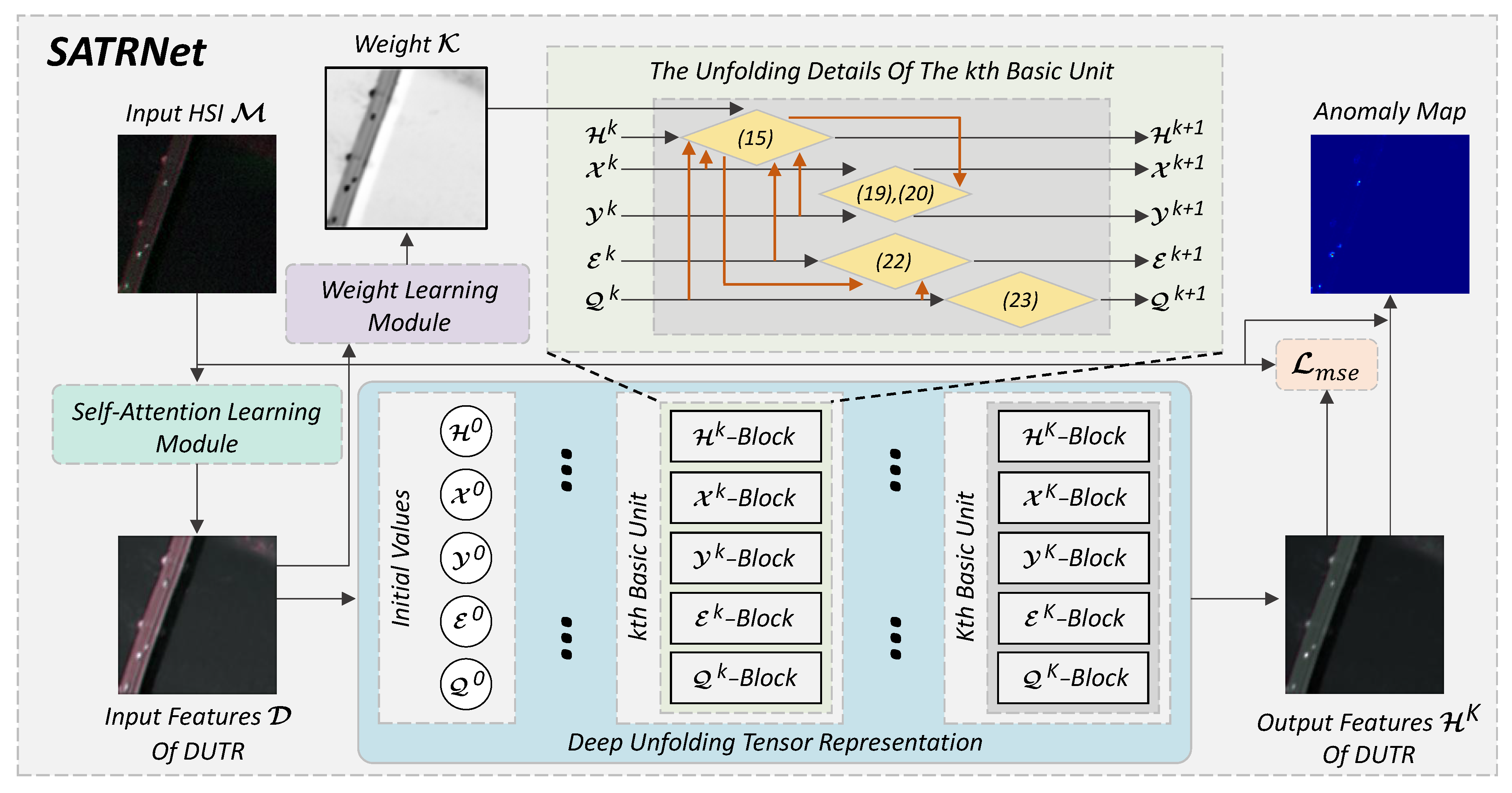
Now, we unfold the above iterative algorithm to build an effective deep network. As shown in Figure 1, DUTR first receives the tensor $\mathcal{D}$ obtained by SALM and then learns local details to produce the weight tensor $\mathcal{K}$ via WLM. Finally, the tensors $\mathcal{D}$ and $\mathcal{K}$ are input into the deep network consisting of K consecutive basic units; the value of K is typically smaller than that of the iteration number for traditional algorithms. Each basic unit in DUTR consists of $\mathcal{H}$-block, $\mathcal{X}$-block, $\mathcal{Y}$-block, $\mathcal{E}$-block, and $\mathcal{Q}$-block, where each block corresponds to a subproblem-solving step in the iterative algorithm. Such a network architecture design gives each module of the network explicit physical meaning, therefore enhancing the network interpretability and essentially alleviating the IM problem. Figure 4 shows the relationship between the optimization algorithms and the design of network blocks more clearly. Each block is regarded as the interpretable mapping of the optimization algorithm, and the basic units formed by the connection of these network blocks form an interpretable network. In addition, unlike traditional ADMM, in which most of the parameters are predefined or calculated manually, all the parameters are learnable and can be updated automatically by the network in the proposed SATRNet. For example, the update of penalty parameter $\mu$ is independent of $\rho$ but is adjusted by backpropagation during the network training process. Similarly, $\lambda$ does not need to be configured manually but is learned adaptively from the network.

3.3. SATRNet for HAD

SATRNet is optimized by the widely used Adam optimizer and the backpropagation strategy. The mean squared error (MSE) is a simple and effective loss function commonly used in HAD [32]. As the objective function for optimization of SATRNet, MSE is given by

$$\begin{array}{c}\hfill {\mathcal{L}}_{mse}={\displaystyle \frac{1}{hw}}\sum _{i=1}^h\sum _{j=1}^w{\parallel ({\mathit{x}}_{i,j}-{\tilde{\mathit{x}}}_{i,j})\parallel }_2^2,\end{array}$$

(24)

where ${\mathit{x}}_{i,j}$ and ${\tilde{\mathit{x}}}_{i,j}$ represent the pixels at location $(i,j)$ of $\mathcal{M}$ and ${\mathcal{H}}^K$. Finally, the anomaly detection map $\mathit{B}$ can be obtained by

$$\begin{array}{c}\hfill \mathit{B}(h,w)=\sqrt{\sum _{i=1}^c{\left|\mathcal{P}(h,w,c)\right|}^2}.\end{array}$$

(25)

where $\mathcal{P}=\mathcal{M}-{\mathcal{H}}^K$.

The SATRNet for HAD is summarized in Algorithm 1.

Algorithm 1 SATRNet

for HAD Input: HSI tensor $\mathcal{M}$, parameter K.    1: Initialize: ${\mathcal{H}}^0={\mathcal{E}}^0={\mathcal{Q}}^0=0,{\mathcal{X}}^0={\mathcal{Y}}^0=1e-1$.    2: Step 1: Training Process:    3: while training process do    4:    Obtain $\mathcal{D}$ by Self-Attention Learning Module;    5:    while $i<K$ do    6:       Update $\mathcal{H}$ by (15);    7:       Update $\mathcal{X}$, $\mathcal{Y}$ by (19) and (20);    8:       Update $\mathcal{E}$ by (22);    9:       Update $\mathcal{Q}$ by (23);    10:      $i=i+1$.    11:   end while    12:   Compute the loss function by (24);    13:   Perform network backward process.    14: end while    15: Step 2: Detection Process:    16: Obtain the low-rank background tensor ${\mathcal{H}}^K$.    17: Obtain the anomaly detection map $\mathit{B}$ by (25).    Output:  Anomaly detection map $\mathit{B}$.

4. Results

In this section, we assess the efficacy of the proposed SATRNet in comparison with a number of advanced HAD methods across 11 HSI datasets.

4.1. Datasets

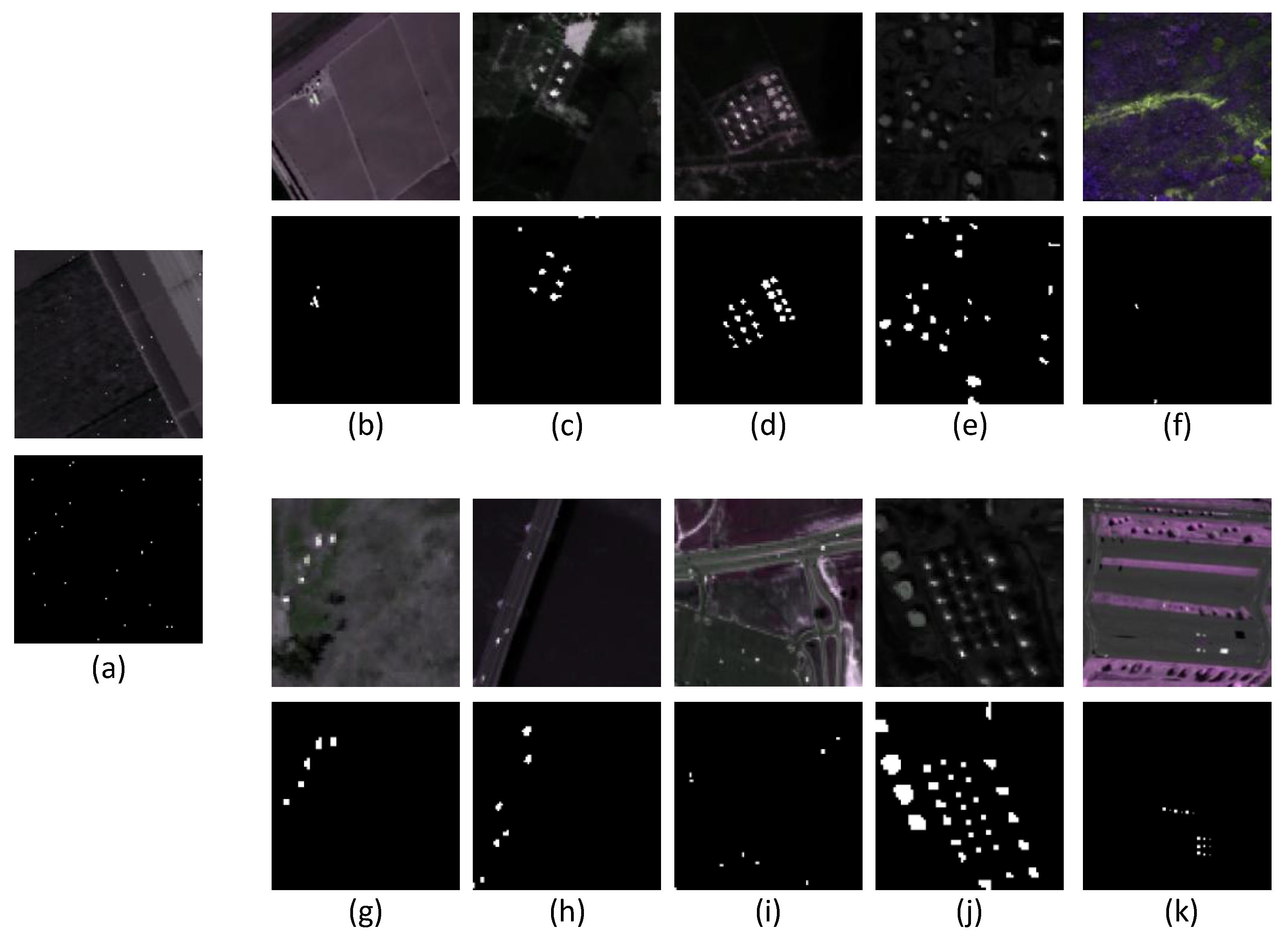
To systematically evaluate the performance of the proposed SATRNet approach, one synthetic and 10 real HSI datasets were employed, where the synthetic Salinas-I dataset was provided by Tan et al. [58]. The Salinas-II dataset was collected in the Salinas Valley, CA, USA, where farmhouses are regarded as anomalies [59]. The Urban-I, Urban-II, and Urban-IV datasets were collected from the widely used ABU dataset [22]. In the Urban-I dataset, multiple storage tanks within an oil refinery are labeled as anomalies. In the Urban-II and Urban-IV datasets, buildings are considered as anomalies. The UHAD dataset [60] is provided by Liu et al. and represents a park scene where pedestrians on the grass are regarded as anomalous, tiny targets. The HAD-100 dataset is a test scene from a large-scale HAD dataset [61] proposed by Li et al., where man-made objects are considered as anomalies. The Pavia dataset [32] was collected in Pavia, Italy, where three cars on the bridge and two patches of bare soil near the bridge-pier are labeled as anomalies. The HYDICE dataset [32] was acquired using the hyperspectral digital imagery collection experiment (HYDICE), and the anomalies are composed of vehicles and roofs under different backgrounds. The anomalies in the Segundo dataset [62] are storage tanks and towers, and the anomaly pixels account for 6.45% of the whole image, which is significantly higher than the above datasets. The background of the SpecTIR dataset [63] is mainly roads and vegetation, while anomalies are composed of man-made colored square textiles of different sizes. The details of these datasets are listed in

Table 1. Detailed information for 11 HSI datasets.

Datasets	Location	Spatial Size	Number of Bands	Sensors	Size of Targets	Proportion
Salinas-I [58]	Salinas Valley	120 × 120	204	AVIRIS	Small	0.17%
Salinas-II [59]	Salinas Valley	150 × 200	204	AVIRIS	Small and large	0.14%
Urban-I [22]	Texas Coast	100 × 100	204	AVIRIS	Small and large	0.67%
Urban-II [22]	Texas Coast	100 × 100	207	AVIRIS	Small and large	1.55%
Urban-IV [22]	Los Angeles	100 × 100	205	AVIRIS	Large	2.72%
UHAD [60]	Park	250 × 250	61	HyperspecI	Small	0.05%
HAD-100 [61]	Grassland	64 × 64	276	AVIRIS-NG	Large	0.65%
Pavia [32]	Pavia	100 × 100	102	ROSIS	Small and large	0.68%
HYDICE [32]	Urban	80 × 100	162	HYDICE	Small	0.23%
Segundo [62]	Segundo	75 × 75	224	AVIRIS	Small and large	6.45%
SpecTIR [63]	New York	180 × 180	120	SHARE	Small and large	0.22%

, and the pseudo-color images and ground truth images are exhibited in Figure 5.

4.2. Compared Methods and Parameter Settings

In the experiments, 7 advanced compared methods were selected to evaluate the detection performance of the developed SATRNet method. These compared methods include two statistical theory-based methods, i.e., RX [6] and 2S-GLRT [64]; one MLRR-based method, i.e., LRASR [13]; three TR-based methods, i.e., PCA-TLRSR [20], CF2-GNBRL [24], and LARTVAD [19]; and two DL-based methods, i.e., Auto-AD [29] and DFAN [32]. All parameters involved in the above compared methods were used according to the authors’ recommended values or tuned to the optimal settings. As shown in

Table 2. Parameter values for the compared methods on the first 6 datasets.

Methods	Parameters	Salinas-I	Salinas-II	Urban-I	Urban-II	Urban-IV	UHAD
RX	/	/	/	/	/	/	/
2S-GLRT	($w_{in}$, $w_{out}$)	(1, 3)	(11, 15)	(11, 13)	(11, 13)	(11, 13)	(11, 13)
LRASR	(p, k, $\lambda$, $\beta$)	(20, 15, 0.1, 0.1)	(20, 15, 0.1, 0.1)	(20, 15, 0.1, 0.01)	(20, 15, 0.1, 0.1)	(20, 15, 0.1, 0.1)	(20, 15, 0.1, 0.1)
PCA-TLRSR	(d, ${\lambda }_1$, ${\lambda }_2$, $\omega$)	(10, 0.06, 0.1, 5)	(5, 0.1, 0.5, 5)	(5, 0.06, 0.1, 5)	(5, 0.06, 0.1, 5)	(10, 0.06, 0.1, 5)	(5, 0.06, 0.01, 5)
LARTVAD	(K, $\lambda$, $\beta$)	(60, 0.1, 2)	(60, 0.1, 2)	(80, 0.1, 0.1)	(80, 0.1, 0.1)	(80, 0.1, 0.1)	(80, 0.1, 0.1)
CF2-GNBRL	($x_{PCA}$, ${\lambda }_1$, ${\lambda }_2$, $\beta$)	(2, 0.01, 0.01, 0.05)	(2, 0.01, 0.01, 0.05)	(2, 0.01, 0.01, 0.05)	(2, 0.01, 0.01, 0.05)	(2, 0.01, 0.01, 0.05)	(5, 0.01, 0.01, 0.05)
Auto-AD	/	/	/	/	/	/	/
DFAN	($MinPts$, $Eps$, $Epochs$, $LR$)	(3, 0.5, 30, 1 × 10−5)	(3, 0.5, 30, 1 × 10−5)	(4, 0.5, 20, 1 × 10−4)	(3, 0.5, 30, 1 × 10−5)	(6, 0.5, 20, 1 × 10−2)	(3, 0.5, 30, 1 × 10−5)

and

Table 3. Parameter values for the compared methods on the last 5 datasets.

Methods	Parameters	HAD-100	Pavia	HYDICE	Segundo	SpecTIR
RX	/	/	/	/	/	/
2S-GLRT	($w_{in}$, $w_{out}$)	(11, 13)	(11, 13)	(11, 13)	(11, 13)	(11, 13)
LRASR	(p, k, $\lambda$, $\beta$)	(20, 15, 0.01, 0.1)	(20, 15, 0.01, 0.1)	(20, 15, 0.01, 0.1)	(20, 15, 0.01, 0.1)	(20, 15, 0.1, 0.1)
PCA-TLRSR	(d, ${\lambda }_1$, ${\lambda }_2$, $\omega$)	(10, 0.06, 0.1, 5)	(10, 0.06, 0.01, 5)	(10, 0.06, 0.01, 5)	(5, 0.06, 0.1, 5)	(5, 0.06, 0.1, 5)
LARTVAD	(K, $\lambda$, $\beta$)	(40, 0.1, 10)	(80, 0.1, 0.1)	(80, 3, 2)	(80, 0.1, 0.1)	(80, 0.1, 0.1)
CF2-GNBRL	(${\lambda }_1$, ${\lambda }_2$, $\beta$)	(5, 0.01, 0.01, 0.05)	(2, 0.01, 0.01, 0.05)	(2, 0.01, 0.01, 0.05)	(2, 0.01, 0.01, 0.05)	(2, 0.01, 0.01, 0.05)
Auto-AD	/	/	/	/	/	/
DFAN	($MinPts$, $Eps$, $Epochs$, $LR$)	(3, 0.5, 30, 1 × 10−5)	(6, 0.6, 20, 1 × 10−4)	(3, 0.5, 30, 1 × 10−2)	(3, 0.5, 30, 1 × 10−5)	(3, 0.5, 30, 1 × 10−5)

, we give the parameter values of all compared algorithms for each dataset.

The proposed SATRNet was computed on NVIDIA GPUs, GeForce RTX 4060, and Intel Core i7 processors, implemented in the Pytorch framework on the Windows 10 operating system. The network was trained using the Adam optimizer, and the hyperparameters were set as follows: the learning rate was 0.001, the batch size was 1, and the training epochs were 300 and 500 for the HYDICE and SpecTIR datasets, respectively, and 100 for the other datasets. In addition, SATRNet involves a key parameter, i.e., the number of basic units K, which is discussed in detail in Section 4.5.

4.3. Detection Performance

The detection performance of each method was evaluated using the receiver operating characteristic (ROC) curve and the area under the ROC curve (AUC) [65]. In addition, 3D-ROCs [66], generated by ROCs and separability box plots, were also introduced to further evaluate detection performance effectively.

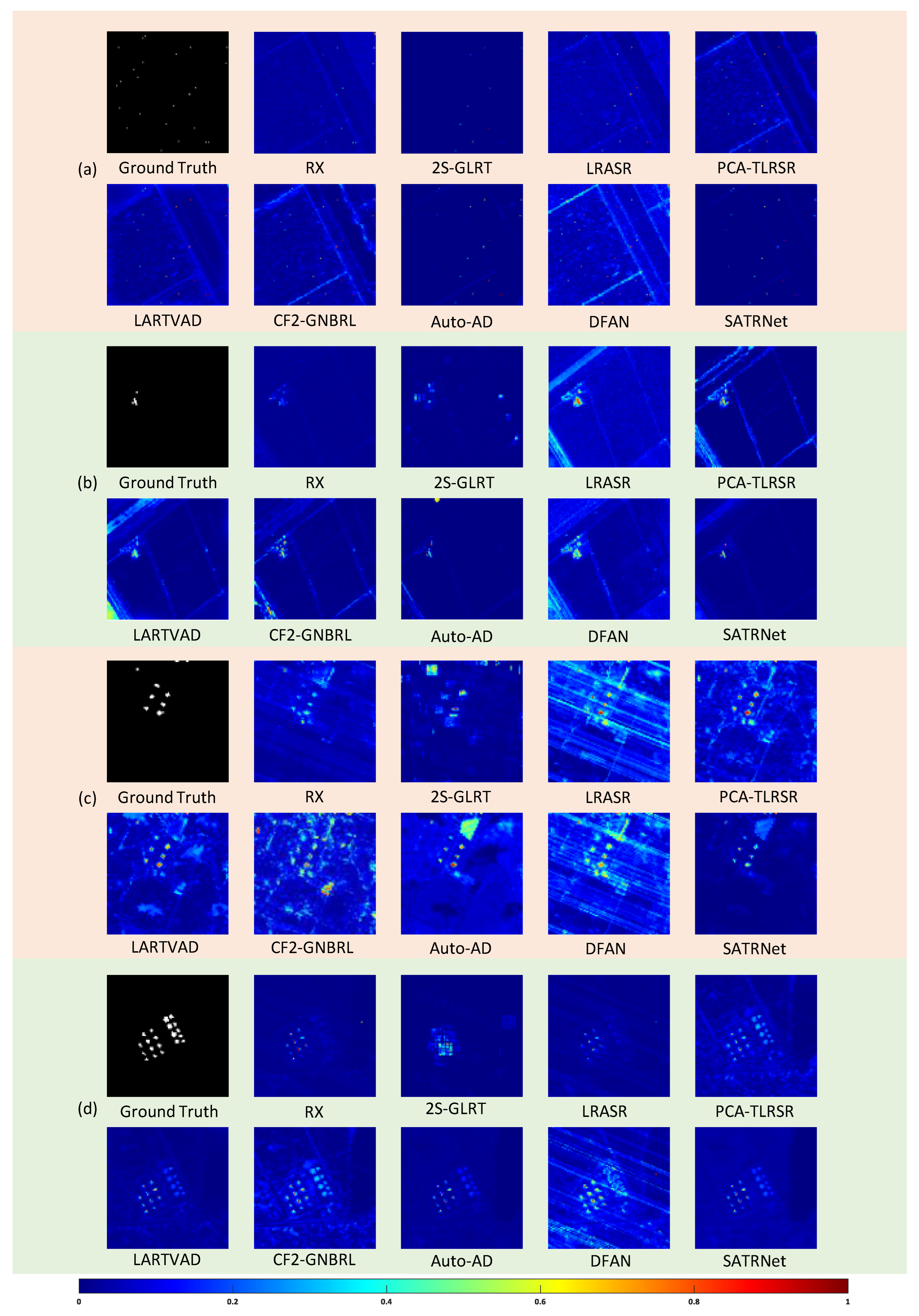
Figure 6, Figure 7 and Figure 8 show the visual detection results of different HAD methods on 11 HSI datasets. The RX detector can detect most anomalies, but it has a dark brightness and slight false alarms. Its performance on the HAD-100 dataset is commendable, with obvious anomalies detected. Overall, the performance of RX is relatively balanced. For the 2S-GLRT algorithm, a few anomalies are correctly detected. The detection map shows erroneous blocky anomalies; this is unacceptable, although the background is relatively pure. This result may be attributed to the sliding dual-window strategy of 2S-GLRT to reduce false alarms, which also makes it unable to handle features of different scales. As a milestone of the MLRR-based method, the detection results of LRASR show that it has poor ability in the degree of background suppression, and on the Urban-I dataset, it suffers serious interference from noise. Owing to the powerful representation capacity of TR, the detection performance of PCA-TLRSR is better than the above algorithms, and more anomalies are detected, but it also suffers from eliminating background information. In terms of visual effects, LARTVAD has good performance, similar to PCA-TLRSR, but its background suppression is slightly better than PCA-TLRSR. CF2-GNBRL has the same limitation on false detections as PCA-TLRSR and LARTVAD, which is more serious on some datasets, such as Urban-I and HAD-100. The detection results of Auto-AD on all datasets show relatively pure backgrounds, but they are affected by the IM issue, and significantly fewer anomalies are detected. Although DFAN can highlight anomalies well, there are lots of false alarms on all datasets, which makes it more difficult to locate anomalies. On the contrary, the proposed SATRNet can greatly reduce the erroneous detection on the background and maintain an appearance similar to the ground truth maps.

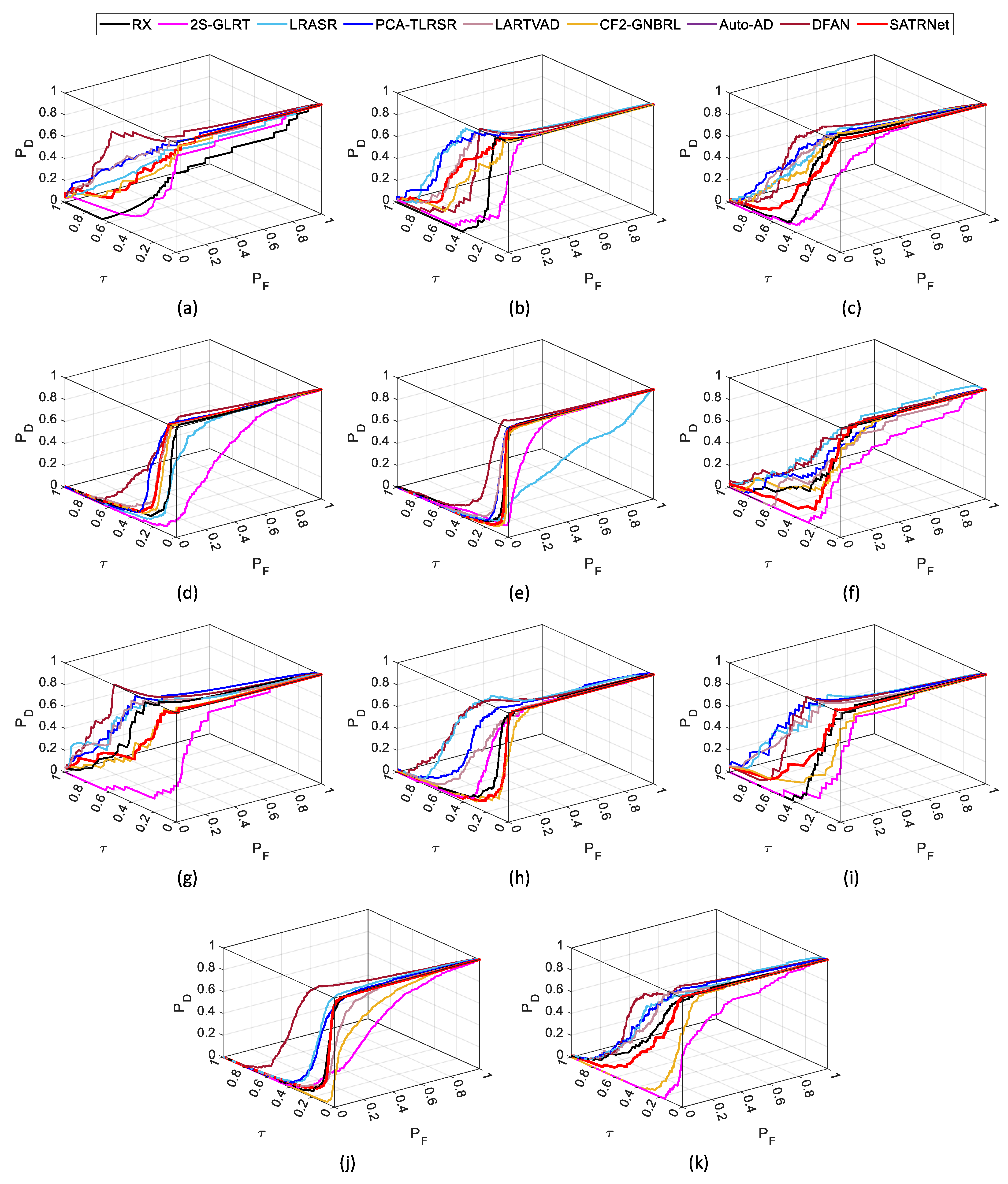
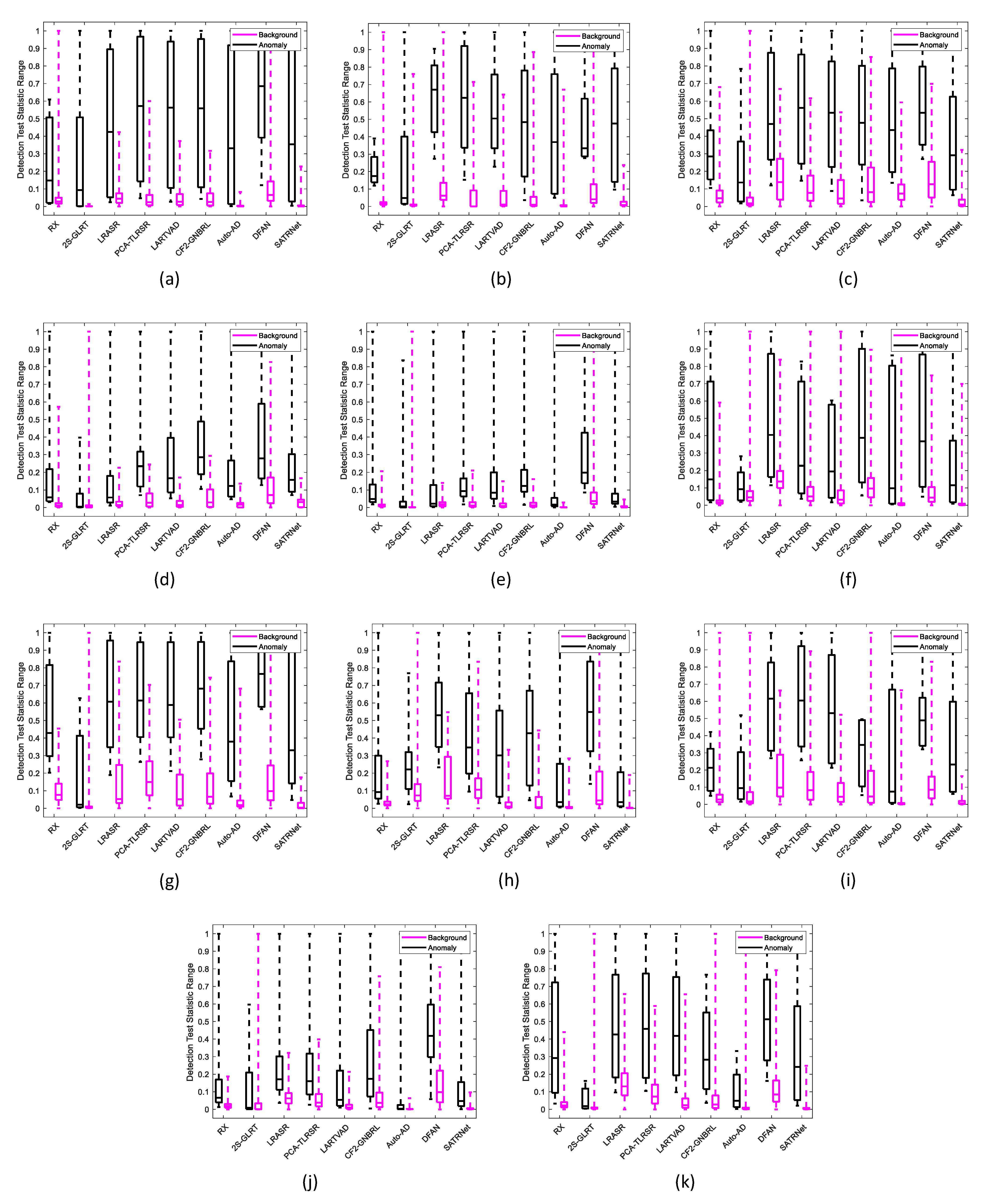
Figure 9 shows the ROC curves of different HAD methods on all datasets. The red curve regarding the proposed SATRNet has both high detection probability $P_D$ and low false alarm probability $P_F$. Therefore, it is closer to the upper left corner than other HAD methods, which stands for excellent HAD performance. Figure 10 shows the 3D-ROC curves obtained by each method on 11 datasets, respectively. As can be seen from Figure 10, the 3D-ROC curves of the SATRNet are closer to the upper right corner than those of other detectors, which means that SATRNet has the best detection performance. Furthermore, Figure 11 shows the box plots of the separation of backgrounds and anomalies by different methods on all datasets. The background boxes (i.e., purple boxes) and anomaly boxes (i.e., black boxes) are displayed by 10% to 90% of the images, and the height of the boxes indicates the degree of background suppression and anomaly detection of different algorithms. It can be seen from Figure 11 that although the gap between the background and anomaly boxes of the proposed method is not always the largest, it achieves the best background suppression without overlapping. In summary, SATRNet exhibits a stronger ability to separate background from anomalies on 11 datasets.

To quantitatively measure the accuracy of the proposed method, the AUC and running time of each method on 11 datasets are listed in

Table 4. Quantitative results over different HAD algorithms on 11 datasets.

Datasets	Metrics	RX	2S-GLRT	LRASR	PCA-TLRSR	LARTVAD	CF2-GNBRL	Auto-AD	DFAN	SATRNet
Salinas-I	AUC	0.8073	0.9296	0.9269	0.9884	0.9780	0.9833	0.9876	0.9913	0.9924
	Time (s)	0.6036	45.9294	60.3541	4.0059	31.1208	150.4626	9.9758	30.9004	13.3504
Salinas-II	AUC	0.9994	0.9754	0.9983	0.9974	0.9945	0.9881	0.9965	0.9677	0.9994
	Time (s)	1.0782	626.3742	58.0547	19.7640	86.0172	212.4481	26.6702	60.4936	26.3504
Urban-I	AUC	0.9907	0.9206	0.9621	0.9892	0.9893	0.9474	0.9844	0.9898	0.9909
	Time (s)	0.4242	134.8021	20.0812	2.2647	24.3573	170.7258	19.7661	32.7611	9.6824
Urban-II	AUC	0.9946	0.7354	0.9482	0.9947	0.9983	0.9968	0.9993	0.9652	0.9994
	Time (s)	0.3719	191.4367	24.3287	2.4378	26.4354	170.4741	9.9373	28.4253	12.5209
Urban-IV	AUC	0.9887	0.9099	0.6120	0.9856	0.9908	0.9952	0.9924	0.9832	0.9965
	Time (s)	0.4025	201.6623	38.7214	2.4194	23.2054	213.9266	6.9560	15.6662	6.4984
UHAD	AUC	0.9759	0.7509	0.9241	0.9194	0.8953	0.9367	0.9640	0.9677	0.9902
	Time (s)	0.0968	823.9238	297.4990	69.4288	231.2874	840.1632	33.8099	98.5544	25.7368
HAD-100	AUC	0.9977	0.8920	0.9816	0.9920	0.9965	0.9931	0.9924	0.9971	0.9977
	Time (s)	0.1885	112.6620	11.4568	1.9148	6.0656	84.7245	21.0011	8.6736	13.5849
Pavia	AUC	0.9887	0.9084	0.9910	0.9665	0.9896	0.9873	0.9732	0.9914	0.9971
	Time (s)	0.0538	140.1739	12.4761	4.7736	24.5325	87.5847	20.8602	27.6034	32.1914
HYDICE	AUC	0.9824	0.8843	0.9742	0.9963	0.9974	0.9216	0.9694	0.9982	0.9986
	Time (s)	0.3047	129.0832	21.2849	4.2619	22.7051	101.1674	23.4645	14.8354	15.6793
Segundo	AUC	0.9753	0.7570	0.9719	0.9576	0.9305	0.9249	0.8701	0.9714	0.9900
	Time (s)	0.2937	115.2845	13.9249	2.4278	15.3215	48.6454	18.4637	16.5910	5.5105
SpecTIR	AUC	0.9914	0.8440	0.9491	0.9889	0.9959	0.9774	0.9719	0.9910	0.9988
	Time (s)	1.1375	410.0467	56.3814	34.3501	175.2243	420.6973	26.2397	43.2219	36.5105

Bold values indicate the best performance results.

, where the best results are shown in bold. From Table 4, it can be seen that SATRNet achieves the highest AUC values on all datasets. For the Salinas-II and HAD-100 datasets, the RX method is tied for first place with our method, but SATRNet is highly competitive due to better background suppression and detection rates in visualization, which is more conducive to accurate anomaly identification. In terms of running time, the RX algorithm has the shortest running time, but the detection results are not satisfactory. Although the time efficiency of the proposed SATRNet ranks middle among all methods, such time cost is acceptable given the excellent HAD ability.

4.4. Ablation Study

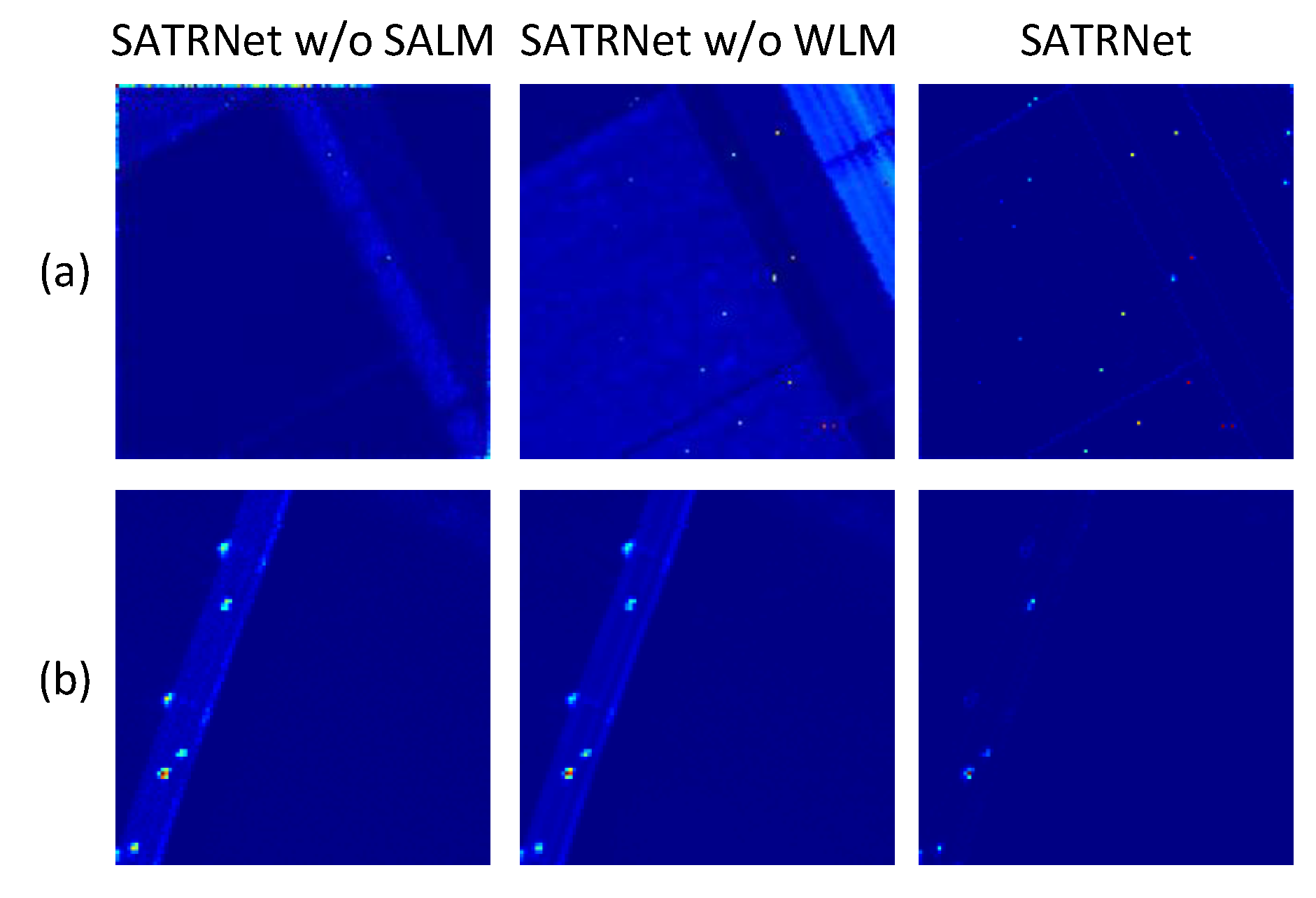
This section studies the effectiveness of the two key components of SATRNet, i.e., SALM and WLM.

Table 5. Quantitative results of ablation experiments on 11 datasets.

Datasets	Metrics	SATRNet w/o SALM	SATRNet w/o WLM	SATRNet
Salinas-I	AUC	0.7599	0.9441	0.9924
	Time (s)	9.9418	12.9921	13.3504
Salinas-II	AUC	0.9998	0.9998	0.9994
	Time (s)	21.2195	23.4119	26.3504
Urban-I	AUC	0.9718	0.9832	0.9909
	Time (s)	7.7756	7.9701	9.6824
Urban-II	AUC	0.9989	0.9993	0.9994
	Time (s)	4.8408	10.9294	12.5209
Urban-IV	AUC	0.3948	0.9964	0.9965
	Time (s)	4.7376	5.5326	6.4984
UHAD	AUC	0.0180	0.9257	0.9902
	Time (s)	20.3288	24.5836	25.7368
HAD-100	AUC	0.7491	0.7457	0.9977
	Time (s)	11.5895	11.1662	13.5849
Pavia	AUC	0.9903	0.9907	0.9971
	Time (s)	29.4589	29.1680	32.1914
HYDICE	AUC	0.7549	0.8463	0.9986
	Time (s)	11.6275	14.7218	15.6793
Segundo	AUC	0.9899	0.9808	0.9900
	Time (s)	4.4982	4.4902	5.5105
SpecTIR	AUC	0.6042	0.8561	0.9988
	Time (s)	39.8812	43.1194	46.5105

Bold values indicate the best performance results.

shows the detection performance of the proposed method with SALM and WLM removed. As can be seen from Table 5, except for the Salinas-II dataset, the detection performance on other datasets has declined to varying degrees after removing SALM. The performance degradation is more significant on Salinas-I, Urban-IV, UHAD, HAD-100, HYDICE, and SpecTIR after removing SALM, among which HAD completely failed on the UHAD dataset; this sufficiently illustrates the importance of SALM in extracting discriminant features for subsequent separation of background and anomalies. Then, we fixed all values in the weight tensor $\mathcal{K}$ of SATRNet to 1 for the method after removing WLM. As shown in Table 5, there is still a decline in detection performance on all datasets except for Salinas-II. This indicates that DUTR may not be able to completely and accurately learn the background features when it loses the local details injected by WLM, thus affecting HAD performance. We provide qualitative results on the Salinas-I and Pavia datasets, as shown in Figure 12. On the Salinas-I dataset, removing SALM makes the method detect fewer anomalies. When removing WLM, the background is falsely detected, which means that WLM is beneficial for more accurate background learning. For the Pavia dataset, removing either SALM or WLM makes the model wrongly detect roads as anomalies. Such results are not surprising and correspond well to the AUC scores. Therefore, we can conclude that both SALM and WLM are crucial for improving detection performance. When incorporating SALM and WLM, SATRNet can achieve excellent HAD performance on 11 datasets, demonstrating the effectiveness and rationality of the proposed method.

4.5. Parameter Analysis

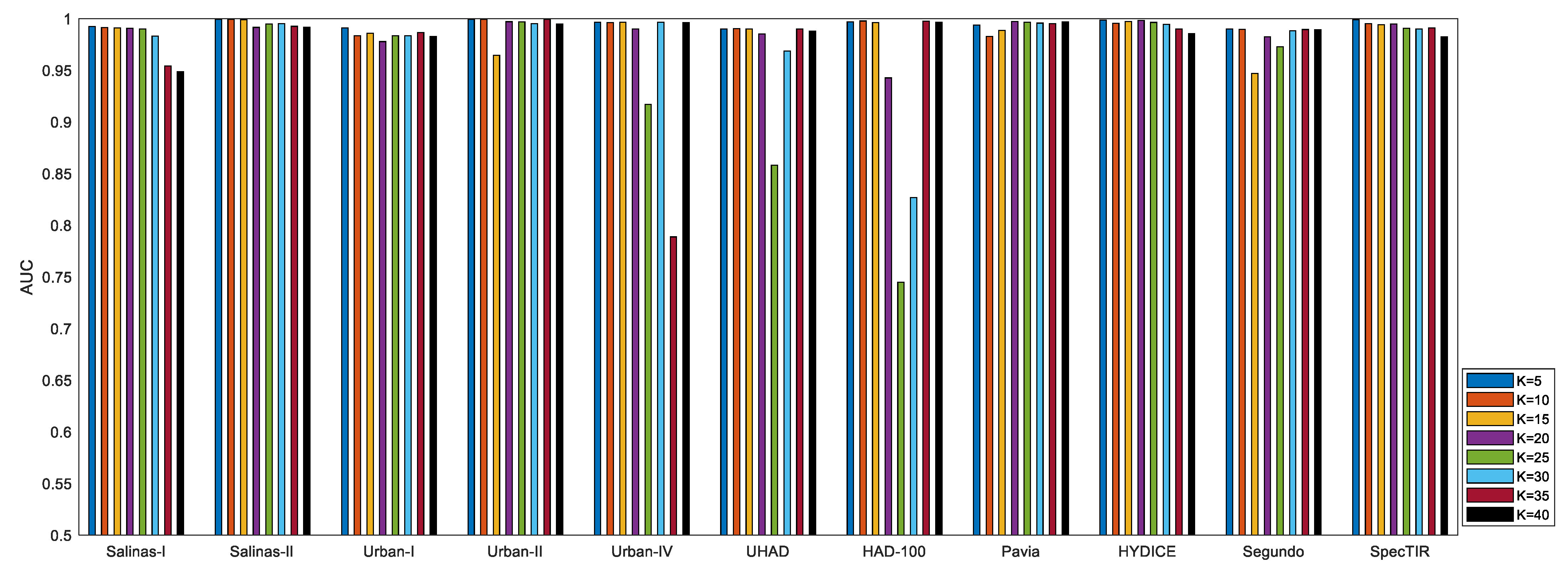
In the proposed SATRNet, the main DUTR part consists of K successive basic units to progressively separate the background and anomalies, corresponding to the iteration times of model-based algorithms. This section investigates the impacts of the number of basic units K on detection performance. Figure 13 shows the detection performance of the proposed method with various values of K on 11 datasets, where the value of K is set as 5, 10, 15, 20, 25, 30, 35, and 40 for each dataset. As shown in Figure 13, the best performance on most of the datasets is produced at $K=5$ and $K=10$, which illustrates that the required iteration times of SATRNet are much less than those of model-based algorithms, showing high efficiency. Therefore, for Salinas-I, Salinas-II, Urban-I, Urban-II, Urban-IV, HYDICE, Segundo, and SpecTIR datasets, the value of K is set as 5; for the UHAD and HAD-100 datasets, the value of K is 10; and for the Pavia dataset, the value of K is set as 20. For future users, to balance time efficiency and detection performance, we suggest setting K as 5.

5. Discussion

Despite the great success that deep learning-based models have achieved in different fields, recent studies reveal that deep learning is vulnerable under adversarial attacks [67]. Szegedy et al. [67] first found that deep neural networks are fragile when facing adversarial examples. Adversarial examples, also called adversarial noises, are generated by adding subtle adversarial perturbations to the original images and showing a similar appearance to the original images visually. In remote sensing, adversarial examples have also been proven to exist and draw people’s attention to the adversarial robustness of networks [68]. As far as we know, this topic in HAD has not been studied yet. Different from traditional noises that bring about visible degradation to images, adversarial noise can make networks output wrong results without being perceived by humans. This may cause serious security problems in some application scenarios [68]. Therefore, it is essential to analyze the adversarial robustness of the HAD methods.

To examine the adversarial robustness of our proposed SATRNet, we initially generated adversarial samples. These samples necessitate the utilization of adversarial attacks against a well-trained model. Goodfellow et al. [69] introduced a potent adversarial attack method, the fast gradient sign method (FGSM). Notably, FGSM is an established and effective attack method capable of theoretically attacking any loss function [69]. Therefore, we used FGSM as the method for obtaining adversarial samples. The samples $x_{adv}$ are obtained through FGSM as follows:

$$\begin{array}{c}\hfill x_{adv}=clip\left(x+ϵ·sign\left({\nabla }_x{\mathcal{L}}_{mse}(\theta ,x,f\left(x\right))\right)\right).\end{array}$$

(26)

where $clip(·)$ clips the pixel values in the image, ${\nabla }_x{\mathcal{L}}_{mse}(\theta ,x,f\left(x\right))$ calculates the gradients of the loss function ${\mathcal{L}}_{mse}(·)$ with respect to the input sample x, $sign(·)$ is the sign function, and parameter $ϵ$ is used to control the attack strength. Further details of the method can be found in [69].

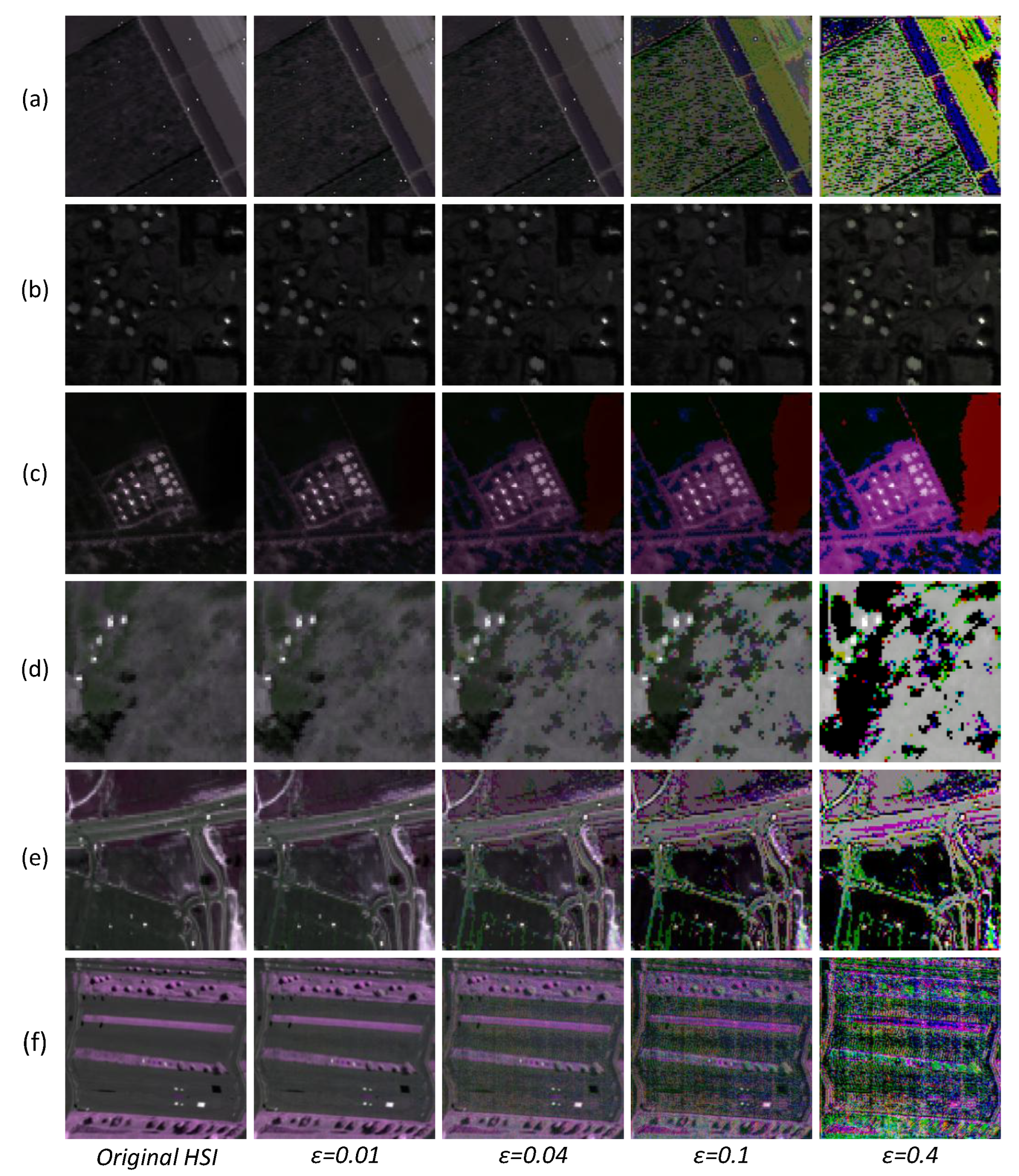
We took 6 HSI datasets to test the adversarial robustness of the proposed method. Figure 14 visualizes the adversarial examples on 6 datasets with different $ϵ$ values. As shown in Figure 14, on 6 datasets, the changes in adversarial examples with $ϵ=0.01$ and $ϵ=0.04$ are hard to perceive compared to clean data. When $ϵ=0.1$ and $ϵ=0.4$, the quality degradation becomes obvious on five datasets, except for Urban-IV. The small-sized anomalies are completely submerged in the background, especially on the Salinas-I, HYDICE, and SpecTIR datasets. For the Urban-IV dataset, as the value of $ϵ$ increases, the quality degradation is relatively not obvious. Combining the above observations, in order to balance attack strength with visual imperceptibility, we selected $ϵ=0.04$ to evaluate adversarial robustness. It is worth mentioning that these observations are basically consistent with those findings in [68,70], where the $ϵ$ value was also set as 0.04.

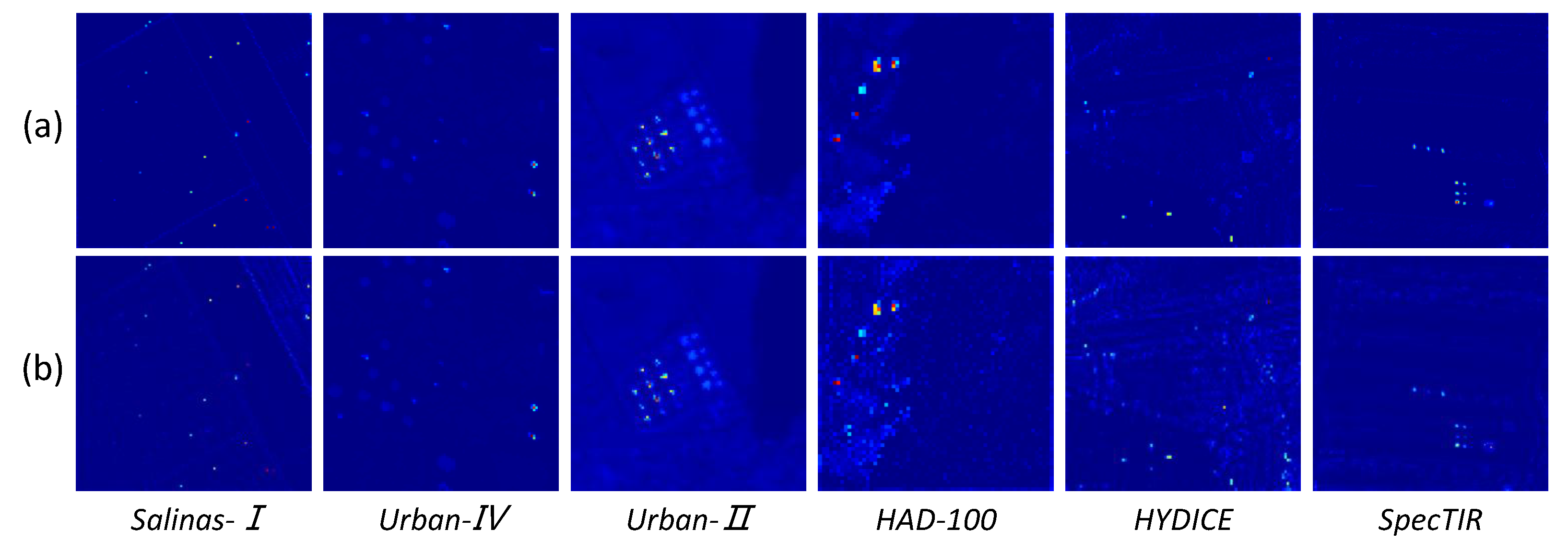
Quantitative performance of the proposed method under different $ϵ$ values on 6 datasets is exhibited in

Table 6. Detection performance ($\mathrm{AUC}$) of the proposed method with different $ϵ$ values.

Datasets	Test Without FGSM	$\mathit{ϵ}=0.01$	$\mathit{ϵ}=0.04$	$\mathit{ϵ}=0.1$	$\mathit{ϵ}=0.4$
Salinas-I	0.9924	0.9933	0.9912	0.9861	0.8761
Urban-IV	0.9965	0.9965	0.9965	0.9965	0.9965
Urban-II	0.9994	0.9994	0.9994	0.9994	0.9987
HAD-100	0.9977	0.9970	0.9907	0.9467	0.7150
HYDICE	0.9986	0.9980	0.9892	0.9480	0.7257
SpecTIR	0.9988	0.9981	0.9918	0.9516	0.7139

Bold values indicate the best performance results.

. As shown in Table 6, on the Salinas-I, HYDICE, SpecTIR, and HAD-100 datasets, the detection performance of the proposed method experienced a continuous decline with the increase in attack strength. Compared to the detection performance on clean images, the performance degradation on the four datasets was not obvious at $ϵ=0.01$ and $ϵ=0.04$. Among them, detection performance on the Salinas-I dataset at $ϵ=0.01$ even exceeded the performance on clean images, which may be caused by the fact that adversarial attacks highlighted small-sized anomalies to some extent while interfering with background learning. At $ϵ=0.1$, the detection performance on the HYDICE, HAD-100, and SpecTIR datasets began to show a large degree of degradation, and at $ϵ=0.4$, the detection results became unsatisfactory. Different from the above results, on the two urban datasets Urban-II and Urban-IV, the proposed method showed almost consistently reliable detection performance under different $ϵ$ values, with only a slight performance degradation on the Urban-II dataset at $ϵ=0.4$, but this is still reliable. The difference in the results can be attributed to the diversity of the surface features of the datasets. Studies have shown that the adversarial robustness of deep neural networks is also related to remote sensing datasets [71]. In general, datasets with higher diversity tend to provide higher robustness when suffering adversarial attacks. The Urban-II and Urban-IV datasets collect urban scenes, which have higher diversity compared to the large patches of grassland in other datasets such as HAD-100. This can be regarded as one possible reason for the difference in performance. Apart from the $\mathrm{AUC}$ index, further comprehensive quantitative analysis is performed using two metrics: ${\mathrm{AUC}}_{\mathrm{BS}}$ [23] and ${\mathrm{AUC}}_{\mathrm{ODP}}$ [23]. ${\mathrm{AUC}}_{\mathrm{BS}}$ focuses on reflecting the background suppression level of the detector, whereas ${\mathrm{AUC}}_{\mathrm{ODP}}$ measures the overall performance of the detection rate and false alarm rate.

Table 7. Background suppression level (${\mathrm{AUC}}_{\mathrm{BS}}$) of the proposed method with different $ϵ$ values.

Datasets	Test Without FGSM	$\mathit{ϵ}=0.01$	$\mathit{ϵ}=0.04$	$\mathit{ϵ}=0.1$	$\mathit{ϵ}=0.4$
Salinas-I	0.9894	0.9894	0.9834	0.9751	0.8761
Urban-IV	0.9927	0.9927	0.9927	0.9927	0.9927
Urban-II	0.9701	0.9700	0.9696	0.9666	0.9987
HAD-100	0.9864	0.9842	0.9702	0.9021	0.6965
HYDICE	0.9892	0.9864	0.9678	0.9315	0.7253
SpecTIR	0.9950	0.9923	0.9820	0.9516	0.7138

Bold values indicate the best performance results.

and

Table 8. Overall performance (${\mathrm{AUC}}_{\mathrm{ODP}}$) of the proposed method with different $ϵ$ values.

Datasets	Test Without FGSM	$\mathit{ϵ}=0.01$	$\mathit{ϵ}=0.04$	$\mathit{ϵ}=0.1$	$\mathit{ϵ}=0.4$
Salinas-I	1.4078	1.4063	1.4071	1.2712	0.8761
Urban-IV	1.4085	1.4085	1.4085	1.4085	1.4085
Urban-II	1.1681	1.1683	1.1698	1.1727	1.0084
HAD-100	1.4414	1.4300	1.3905	1.2861	0.7210
HYDICE	1.3212	1.3157	1.2814	1.0531	0.7256
SpecTIR	1.2826	1.2788	1.1708	0.9517	0.7139

Bold values indicate the best performance results.

show the ${\mathrm{AUC}}_{\mathrm{BS}}$ and ${\mathrm{AUC}}_{\mathrm{ODP}}$ of the proposed method with different $ϵ$ values, respectively. From Table 7 and Table 8, it is not difficult to see that adversarial attacks have a negative impact on the background suppression capability and overall performance of the detector, which is similar to what is reflected by the AUC values. To investigate the adversarial robustness of the proposed method, we further studied the detection performance of $ϵ=0.04$. Figure 15 shows the visual detection results of the 6 datasets when $ϵ=0.04$. As shown in Figure 15, the visual detection effects of the Urban-II and Urban-IV datasets remain basically unchanged, and on other datasets, compared with the original detection results, a small number of false detections appear in the background area of the detection map. However, under the adversarial attack, the visual effect still maintains strong discrimination ability. The above results indicate that, despite the difficulties brought by adversarial attacks to the HAD problem, the proposed SATRNet method maintains strong detection performance under reasonable attack intensity and presents good visual effects.

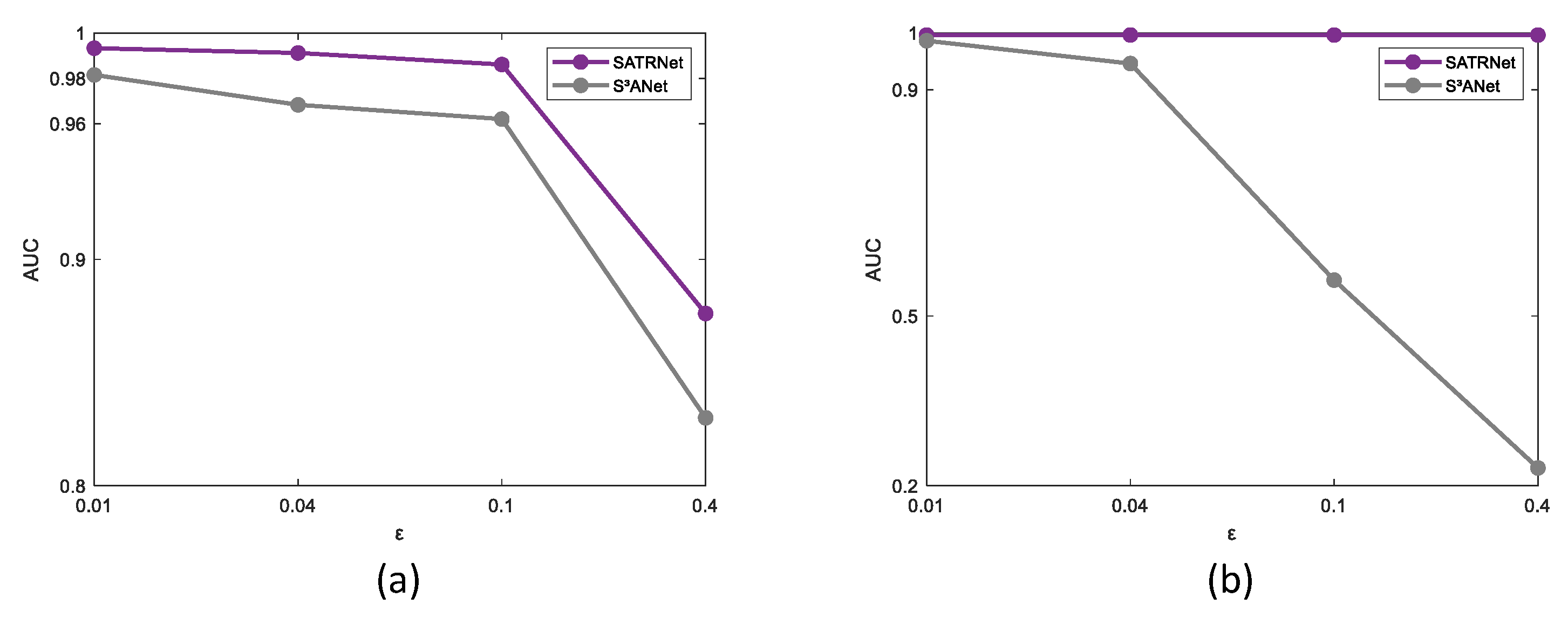
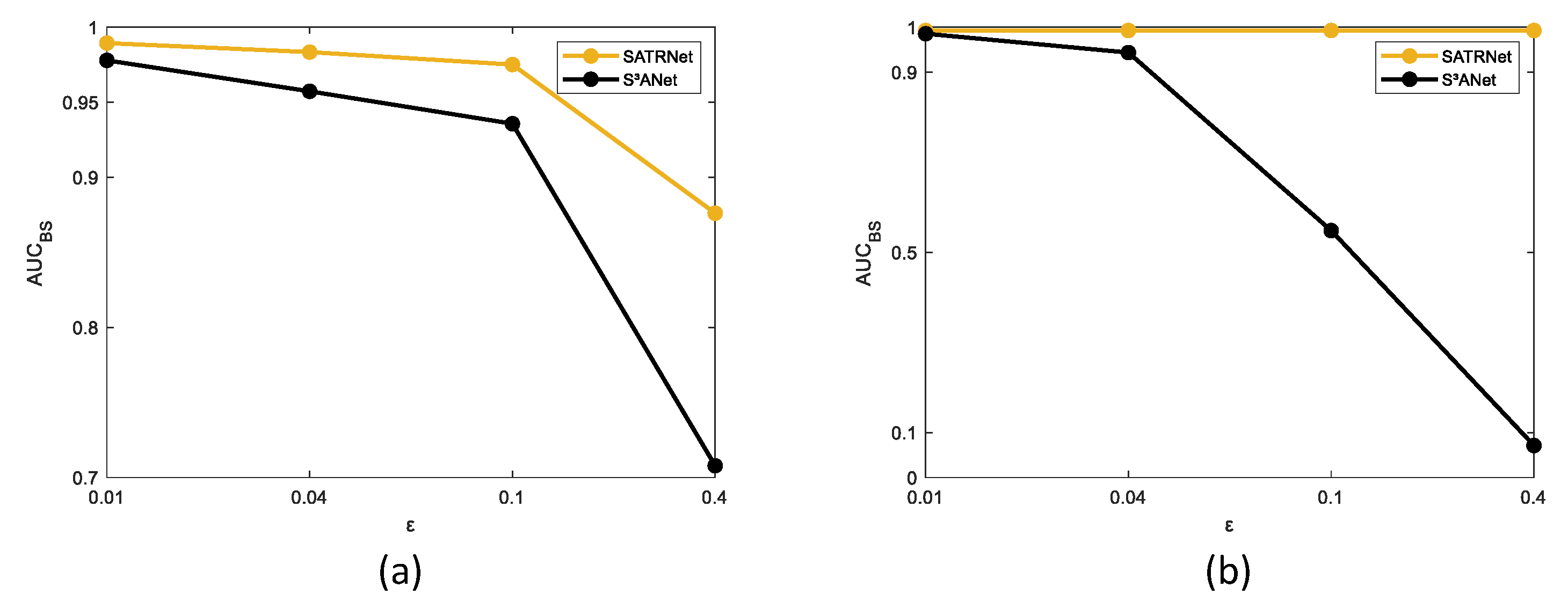
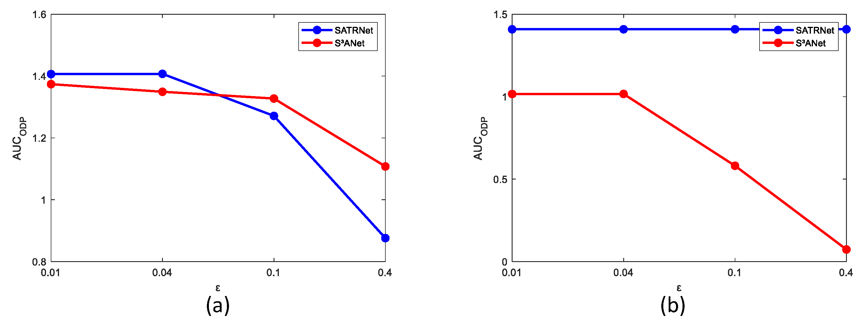
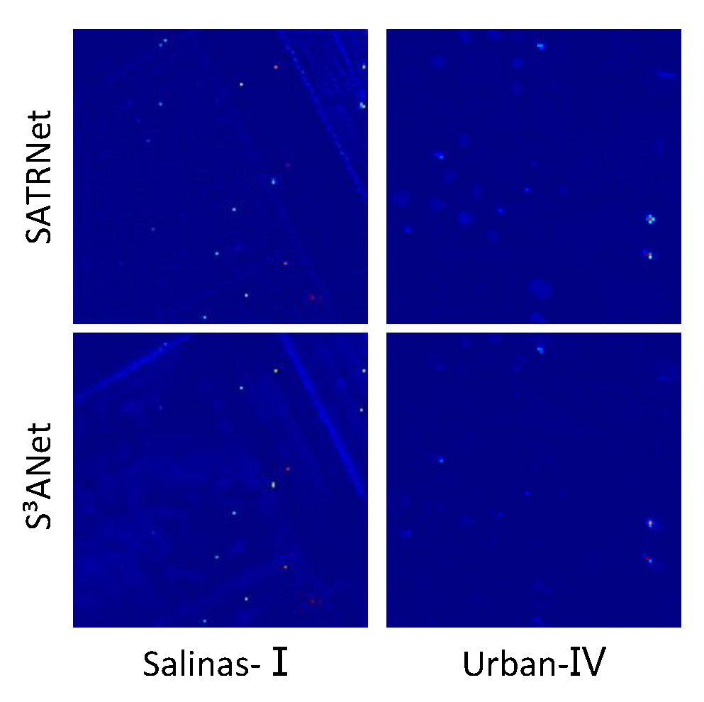
To more comprehensively evaluate the robustness of the proposed algorithm, we compared SATRNet with S³ANet [70], a recently proposed classification network with strong adversarial robustness. The original S³ANet is designed for hyperspectral image classification, which is a supervised method and is inherently different from the unsupervised HAD problem in this work. In order to fit its structure and learning learning paradigm to the HAD task, we made the following modifications. Firstly, in the original S³ANet, the number of output channels is the number of categories; we adjusted it to the number of bands of the input image so as to maintain the consistency of input and output dimensions. Secondly, the loss function was replaced by the MSE regression loss to optimize the reconstruction quality. This adjustment enables S³ANet to reconstruct the background of hyperspectral images in an unsupervised manner and, thus, achieve anomaly detection through residual operation. In the training phase, the batch size was 1, the learning rate was 0.001, and the iteration was 100 rounds. Figure 16 shows the performance of S³ANet on the Salinas-I and Urban-IV datasets when $ϵ=0.04$. It can be seen from Figure 16 that S³ANet experiences a significant decline in various detection indicators on the Salinas-I and Urban-IV datasets, where the performance degradation on the Urban-IV dataset is more significant. As shown in Figure 17, Figure 18 and Figure 19, the AUC, ${\mathrm{AUC}}_{\mathrm{BS}}$, and ${\mathrm{AUC}}_{\mathrm{ODP}}$ metrics under different $ϵ$ values were tested on the Salinas-I and Urban-IV datasets, respectively. The experimental results show that the proposed method performs better in most cases when compared with S³ANet in terms of different AUC metrics on the Salinas-I dataset. On the Urban-IV dataset, the performance of S³ANet declines seriously as the attack strength increases, while the proposed SATRNet method maintains stability in all metrics, showing its significant superiority to the performance of S³ANet. Detection maps of the two methods at $ϵ=0.04$ are given in Figure 20, which also shows that the proposed SATRNet exhibits better detection accuracy. Combining all observations, we can consider that the proposed method has certain adversarial robustness. This benefits from the capture of spatial correlation by self-attention learning and the inherent robustness of the tensor model [72].

6. Conclusions

This paper presents a self-attention-aided deep unfolding tensor representation network (SATRNet) for HAD. SATRNet introduces SALM to extract discriminative features to reduce the difficulty of the following separation of background and anomalies. Then, we formulated the HAD problem as the TR problem, which is further guided by the weight tensor $\mathcal{K}$ generated by WLM to inject local details into the model. By unfolding and parameterizing this TR algorithm, DUTR has K consecutive basic units with precise correspondence to the iterative algorithm, ensuring seamless integration of model-based methods and learning-based methods. Combining the merits of model-based and learning-based paradigms, SATRNet can effectively alleviate the IM problem, leading to the best performance on 11 datasets. Note that SATRNet is resistant to adversarial attacks, which also represents the first work to investigate adversarial robustness in HAD.

References

1. Chen, X.; Wang, Z.; Wang, K.; Jia, H.; Han, Z.; Tang, Y. Multi-dimensional low-rank with weighted Schatten p-norm minimization for hyperspectral anomaly detection. Remote Sens. 2023, 16, 74. [Google Scholar] [CrossRef]
2. Zhao, R.; Yang, Z.; Meng, X.; Shao, F. A novel fully convolutional auto-encoder based on dual clustering and latent feature adversarial consistency for hyperspectral anomaly detection. Remote Sens. 2024, 16, 717. [Google Scholar] [CrossRef]
3. Yin, C.; Lv, X.; Zhang, L.; Ma, L.; Wang, H.; Zhang, L.; Zhang, Z. Hyperspectral UAV images at different altitudes for monitoring the leaf nitrogen content in cotton crops. Remote Sens. 2022, 14, 2576. [Google Scholar] [CrossRef]
4. Farrar, M.B.; Wallace, H.M.; Brooks, P.; Yule, C.M.; Tahmasbian, I.; Dunn, P.K.; Hosseini Bai, S. A performance evaluation of Vis/NIR hyperspectral imaging to predict curcumin concentration in fresh turmeric rhizomes. Remote Sens. 2021, 13, 1807. [Google Scholar] [CrossRef]
5. Zhang, X.; Han, L.; Dong, Y.; Shi, Y.; Huang, W.; Han, L.; González-Moreno, P.; Ma, H.; Ye, H.; Sobeih, T. A deep learning-based approach for automated yellow rust disease detection from high-resolution hyperspectral UAV images. Remote Sens. 2019, 11, 1554. [Google Scholar] [CrossRef]
6. Reed, I.S.; Yu, X. Adaptive multiple-band CFAR detection of an optical pattern with unknown spectral distribution. IEEE Trans. Acoust. Speech Signal Process. 1990, 38, 1760–1770. [Google Scholar] [CrossRef]
7. Borghys, D.; Kåsen, I.; Achard, V.; Perneel, C. Comparative evaluation of hyperspectral anomaly detectors in different types of background. In Proceedings of the Algorithms and Technologies for Multispectral, Hyperspectral, and Ultraspectral Imagery XVIII, Baltimore, MD, USA, 23–27 April 2012; pp. 803–814. [Google Scholar]
8. Guo, Q.; Zhang, B.; Ran, Q.; Gao, L.; Li, J.; Plaza, A. Weighted-RXD and linear filter-based RXD: Improving background statistics estimation for anomaly detection in hyperspectral imagery. IEEE J. Sel. Top. Appl. Earth Obs. Remote Sens. 2014, 7, 2351–2366. [Google Scholar] [CrossRef]
9. Kwon, H.; Nasrabadi, N.M. Kernel RX-algorithm: A nonlinear anomaly detector for hyperspectral imagery. IEEE Trans. Geosci. Remote Sens. 2005, 43, 388–397. [Google Scholar] [CrossRef]
10. Chang, C.-I. Hyperspectral anomaly detection: A dual theory of hyperspectral target detection. IEEE Trans. Geosci. Remote Sens. 2021, 60, 1–20. [Google Scholar] [CrossRef]
11. Li, J.; Zhang, H.; Zhang, L.; Ma, L. Hyperspectral anomaly detection by the use of background joint sparse representation. IEEE J. Sel. Top. Appl. Earth Obs. Remote Sens. 2015, 8, 2523–2533. [Google Scholar] [CrossRef]
12. Zhao, G.; Li, F.; Zhang, X.; Laakso, K.; Chan, J.C.-W. Archetypal analysis and structured sparse representation for hyperspectral anomaly detection. Remote Sens. 2021, 13, 4102. [Google Scholar] [CrossRef]
13. Xu, Y.; Wu, Z.; Li, J.; Plaza, A.; Wei, Z. Anomaly detection in hyperspectral images based on low-rank and sparse representation. IEEE Trans. Geosci. Remote Sens. 2015, 54, 1990–2000. [Google Scholar] [CrossRef]
14. Cheng, T.; Wang, B. Graph and total variation regularized low-rank representation for hyperspectral anomaly detection. IEEE Trans. Geosci. Remote Sens. 2019, 58, 391–406. [Google Scholar] [CrossRef]
15. Ren, L.; Gao, L.; Wang, M.; Sun, X.; Chanussot, J. HADGSM: A unified nonconvex framework for hyperspectral anomaly detection. IEEE Trans. Geosci. Remote Sens. 2024, 62, 5503415. [Google Scholar] [CrossRef]
16. Shang, W.; Jouni, M.; Wu, Z.; Xu, Y.; Dalla Mura, M.; Wei, Z. Hyperspectral anomaly detection based on regularized background abundance tensor decomposition. Remote Sens. 2023, 15, 1679. [Google Scholar] [CrossRef]
17. Shang, W.; Peng, J.; Wu, Z.; Xu, Y.; Jouni, M.; Dalla Mura, M.; Wei, Z. Hyperspectral anomaly detection via sparsity of core tensor under gradient domain. IEEE Trans. Geosci. Remote Sens. 2023, 61, 5517816. [Google Scholar] [CrossRef]
18. Feng, M.; Chen, W.; Yang, Y.; Shu, Q.; Li, H.; Huang, Y. Hyperspectral anomaly detection based on tensor ring decomposition with factors TV regularization. IEEE Trans. Geosci. Remote Sens. 2023, 61, 5514114. [Google Scholar] [CrossRef]
19. Sun, S.; Liu, J.; Chen, X.; Li, W.; Li, H. Hyperspectral anomaly detection with tensor average rank and piecewise smoothness constraints. IEEE Trans. Neural Netw. Learn. Syst. 2022, 34, 8679–8692. [Google Scholar] [CrossRef]
20. Wang, M.; Wang, Q.; Hong, D.; Roy, S.K.; Chanussot, J. Learning tensor low-rank representation for hyperspectral anomaly detection. IEEE Trans. Cybern. 2022, 53, 679–691. [Google Scholar] [CrossRef] [PubMed]
21. Sun, S.; Liu, J.; Li, W. Spatial invariant tensor self-representation model for hyperspectral anomaly detection. IEEE Trans. Cybern. 2023, 54, 3120–3131. [Google Scholar] [CrossRef] [PubMed]
22. Qin, H.; Shen, Q.; Zeng, H.; Chen, Y.; Lu, G. Generalized nonconvex low-rank tensor representation for hyperspectral anomaly detection. IEEE Trans. Geosci. Remote Sens. 2023, 61, 5526612. [Google Scholar] [CrossRef]
23. Yang, J.; Zhao, J.; Chen, L.; Geng, H.; Zhang, P. Learning nonconvex tensor representation with generalized reweighted sparse regularization for hyperspectral anomaly detection. IEEE J. Sel. Top. Appl. Earth Obs. Remote Sens. 2025, 18, 14718–14737. [Google Scholar] [CrossRef]
24. Yu, Q.; Bai, M. Generalized nonconvex hyperspectral anomaly detection via background representation learning with dictionary constraint. SIAM J. Imaging Sci. 2024, 17, 917–950. [Google Scholar] [CrossRef]
25. Chen, L.; Li, Z.; Lu, Z.; Wang, Y.; Nie, H.; Yang, C. Domain-invariant feature learning via margin and structure priors for robotic grasping. IEEE Robot. Autom. Lett. 2024, 10, 1313–1320. [Google Scholar] [CrossRef]
26. Li, J.; Zheng, K.; Gao, L.; Han, Z.; Li, Z.; Chanussot, J. Enhanced deep image prior for unsupervised hyperspectral image super-resolution. IEEE Trans. Geosci. Remote Sens. 2025, 63, 5504218. [Google Scholar] [CrossRef]
27. Li, J.; Zheng, K.; Gao, L.; Ni, L.; Huang, M.; Chanussot, J. Model-informed multistage unsupervised network for hyperspectral image super-resolution. IEEE Trans. Geosci. Remote Sens. 2024, 62, 5516117. [Google Scholar] [CrossRef]
28. Li, Q.; Gong, M.; Yuan, Y.; Wang, Q. Symmetrical feature propagation network for hyperspectral image super-resolution. IEEE Trans. Geosci. Remote Sens. 2022, 60, 5536912. [Google Scholar] [CrossRef]
29. Wang, S.; Wang, X.; Zhang, L.; Zhong, Y. Auto-AD: Autonomous hyperspectral anomaly detection network based on fully convolutional autoencoder. IEEE Trans. Geosci. Remote Sens. 2021, 60, 5503314. [Google Scholar] [CrossRef]
30. Fan, G.; Ma, Y.; Mei, X.; Fan, F.; Huang, J.; Ma, J. Hyperspectral anomaly detection with robust graph autoencoders. IEEE Trans. Geosci. Remote Sens. 2021, 60, 5511314. [Google Scholar]
31. Wu, Z.; Wang, B. Transformer-based autoencoder framework for nonlinear hyperspectral anomaly detection. IEEE Trans. Geosci. Remote Sens. 2024, 62, 5508015. [Google Scholar] [CrossRef]
32. Cheng, X.; Huo, Y.; Lin, S.; Dong, Y.; Zhao, S.; Zhang, M.; Wang, H. Deep feature aggregation network for hyperspectral anomaly detection. IEEE Trans. Instrum. Meas. 2024, 73, 5033016. [Google Scholar] [CrossRef]
33. Lian, J.; Wang, L.; Sun, H.; Huang, H. GT-HAD: Gated transformer for hyperspectral anomaly detection. IEEE Trans. Neural Netw. Learn. Syst. 2024, 36, 3631–3645. [Google Scholar] [CrossRef]
34. Xiao, S.; Zhang, T.; Xu, Z.; Qu, J.; Hou, S.; Dong, W. Anomaly detection of hyperspectral images based on transformer with spatial–spectral dual-window mask. IEEE J. Sel. Top. Appl. Earth Obs. Remote Sens. 2023, 16, 1414–1426. [Google Scholar] [CrossRef]
35. Wang, D.; Zhuang, L.; Gao, L.; Sun, X.; Zhao, X.; Plaza, A. Sliding dual-window-inspired reconstruction network for hyperspectral anomaly detection. IEEE Trans. Geosci. Remote Sens. 2024, 62, 5504115. [Google Scholar] [CrossRef]
36. Yang, Z.; Zhao, R.; Meng, X.; Yang, G.; Sun, W.; Zhang, S.; Li, J. A multi-scale mask convolution-based blind-spot network for hyperspectral anomaly detection. Remote Sens. 2024, 16, 3036. [Google Scholar] [CrossRef]
37. Wang, D.; Zhuang, L.; Gao, L.; Sun, X.; Huang, M.; Plaza, A.J. PDBSNet: Pixel-shuffle downsampling blind-spot reconstruction network for hyperspectral anomaly detection. IEEE Trans. Geosci. Remote Sens. 2023, 61, 5511914. [Google Scholar] [CrossRef]
38. Wang, D.; Zhuang, L.; Gao, L.; Sun, X.; Huang, M.; Plaza, A. BockNet: Blind-block reconstruction network with a guard window for hyperspectral anomaly detection. IEEE Trans. Geosci. Remote Sens. 2023, 61, 5531916. [Google Scholar] [CrossRef]
39. Lu, C.; Feng, J.; Chen, Y.; Liu, W.; Lin, Z.; Yan, S. Tensor robust principal component analysis with a new tensor nuclear norm. IEEE Trans. Pattern Anal. Mach. Intell. 2019, 42, 925–938. [Google Scholar] [CrossRef]
40. Chan, S.H.; Wang, X.; Elgendy, O.A. Plug-and-play ADMM for image restoration: Fixed-point convergence and applications. IEEE Trans. Comput. Imaging 2016, 3, 84–98. [Google Scholar] [CrossRef]
41. He, X.; Wu, J.; Ling, Q.; Li, Z.; Lin, Z.; Zhou, S. Anomaly detection for hyperspectral imagery via tensor low-rank approximation with multiple subspace learning. IEEE Trans. Geosci. Remote Sens. 2023, 61, 5509917. [Google Scholar] [CrossRef]
42. Khader, A.; Yang, J.; Xiao, L. NMF-DuNet: Nonnegative matrix factorization inspired deep unrolling networks for hyperspectral and multispectral image fusion. IEEE J. Sel. Top. Appl. Earth Obs. Remote Sens. 2022, 15, 5704–5720. [Google Scholar] [CrossRef]
43. Qu, J.; Dong, W.; Li, Y.; Hou, S.; Du, Q. An interpretable unsupervised unrolling network for hyperspectral pansharpening. IEEE Trans. Cybern. 2023, 53, 7943–7956. [Google Scholar] [CrossRef]
44. Wang, K.; Liao, X.; Li, J.; Meng, D.; Wang, Y. Hyperspectral image super-resolution via knowledge-driven deep unrolling and transformer embedded convolutional recurrent neural network. IEEE Trans. Image Process. 2023, 32, 4581–4594. [Google Scholar] [CrossRef]
45. Yang, Y.; Sun, J.; Li, H.; Xu, Z. ADMM-CSNet: A deep learning approach for image compressive sensing. IEEE Trans. Pattern Anal. Mach. Intell. 2018, 42, 521–538. [Google Scholar] [CrossRef] [PubMed]
46. Li, C.; Zhang, B.; Hong, D.; Yao, J.; Chanussot, J. LRR-Net: An interpretable deep unfolding network for hyperspectral anomaly detection. IEEE Trans. Geosci. Remote Sens. 2023, 61, 5513412. [Google Scholar] [CrossRef]
47. Lin, S.; Cheng, X.; Zeng, Y.; Huo, Y.; Zhang, M.; Wang, H. Low-rank and sparse representation inspired interpretable network for hyperspectral anomaly detection. IEEE Trans. Instrum. Meas. 2024, 73, 5033116. [Google Scholar] [CrossRef]
48. Wang, L.; Wang, X.; Vizziello, A.; Gamba, P. RSAAE: Residual self-attention-based autoencoder for hyperspectral anomaly detection. IEEE Trans. Geosci. Remote Sens. 2023, 61, 5510614. [Google Scholar] [CrossRef]
49. Tu, B.; Zhou, T.; Liu, B.; He, Y.; Li, J.; Plaza, A. Multi-scale autoencoder suppression strategy for hyperspectral image anomaly detection. IEEE Trans. Image Process. 2023. online ahead of print. [Google Scholar] [CrossRef]
50. Li, Q.; Yuan, Y.; Jia, X.; Wang, Q. Dual-stage approach toward hyperspectral image super-resolution. IEEE Trans. Image Process. 2022, 31, 7252–7263. [Google Scholar] [CrossRef]
51. Li, Q.; Yuan, Y.; Wang, Q. Multiscale factor joint learning for hyperspectral image super-resolution. IEEE Trans. Geosci. Remote Sens. 2023, 61, 5523110. [Google Scholar] [CrossRef]
52. Li, J.; Zheng, K.; Li, Z.; Gao, L.; Jia, X. X-shaped interactive autoencoders with cross-modality mutual learning for unsupervised hyperspectral image super-resolution. IEEE Trans. Geosci. Remote Sens. 2023, 61, 5518317. [Google Scholar] [CrossRef]
53. Chen, L.; Niu, M.; Yang, J.; Qian, Y.; Li, Z.; Wang, K.; Yan, T.; Huang, P. Robotic grasp detection using structure prior attention and multiscale features. IEEE Trans. Syst. Man Cybern. Syst. 2024, 54, 7039–7053. [Google Scholar] [CrossRef]
54. Li, Y.; Zhang, K.; Cao, J.; Timofte, R.; Van Gool, L. Localvit: Bringing locality to vision transformers. arXiv 2021, arXiv:2104.05707. [Google Scholar]
55. Mercer, J. Xvi. functions of positive and negative type, and their connection the theory of integral equations. Philos. Trans. R. Soc. Lond. Ser. A Contain. Pap. A Math. Phys. Character 1909, 209, 415–446. [Google Scholar]
56. Zhang, M.; Zhang, C.; Zhang, Q.; Guo, J.; Gao, X.; Zhang, J. ESSAformer: Efficient transformer for hyperspectral image super-resolution. In Proceedings of the IEEE/CVF International Conference on Computer Vision, Paris, France, 2–3 October 2023; pp. 23073–23084. [Google Scholar]
57. Hendrycks, D.; Gimpel, K. Gaussian error linear units (gelus). arXiv 2016, arXiv:1606.08415. [Google Scholar]
58. Tan, K.; Hou, Z.; Wu, F.; Du, Q.; Chen, Y. Anomaly detection for hyperspectral imagery based on the regularized subspace method and collaborative representation. Remote Sens. 2019, 11, 1318. [Google Scholar] [CrossRef]
59. Zhang, W.; Lu, X.; Li, X. Similarity constrained convex nonnegative matrix factorization for hyperspectral anomaly detection. IEEE Trans. Geosci. Remote Sens. 2019, 57, 4810–4822. [Google Scholar] [CrossRef]
60. Liu, S.; Peng, L.; Chang, X.; Wen, G.; Zhu, C. Adaptive dual-domain learning for hyperspectral anomaly detection with state space models. IEEE Trans. Geosci. Remote Sens. 2025, 63, 5503719. [Google Scholar] [CrossRef]
61. Li, Z.; Wang, Y.; Xiao, C.; Ling, Q.; Lin, Z.; An, W. You only train once: Learning a general anomaly enhancement network with random masks for hyperspectral anomaly detection. IEEE Trans. Geosci. Remote Sens. 2023, 61, 1–18. [Google Scholar] [CrossRef]
62. Sun, B.; Zhao, Z.; Liu, D.; Gao, X.; Yu, T. Tensor decomposition-inspired convolutional autoencoders for hyperspectral anomaly detection. IEEE J. Sel. Top. Appl. Earth Obs. Remote Sens. 2022, 15, 4990–5000. [Google Scholar] [CrossRef]
63. Li, L.; Li, W.; Qu, Y.; Zhao, C.; Tao, R.; Du, Q. Prior-based tensor approximation for anomaly detection in hyperspectral imagery. IEEE Trans. Neural Netw. Learn. Syst. 2020, 33, 1037–1050. [Google Scholar] [CrossRef]
64. Liu, J.; Hou, Z.; Li, W.; Tao, R.; Orlando, D.; Li, H. Multipixel anomaly detection with unknown patterns for hyperspectral imagery. IEEE Trans. Neural Netw. Learn. Syst. 2021, 33, 5557–5567. [Google Scholar] [CrossRef]
65. Chang, C.-I. Comprehensive analysis of receiver operating characteristic (roc) curves for hyperspectral anomaly detection. IEEE Trans. Geosci. Remote Sens. 2022, 60, 5541124. [Google Scholar] [CrossRef]
66. Chang, C.-I. An effective evaluation tool for hyperspectral target detection: 3D receiver operating characteristic curve analysis. IEEE Trans. Geosci. Remote Sens. 2020, 59, 5131–5153. [Google Scholar] [CrossRef]
67. Szegedy, C.; Zaremba, W.; Sutskever, I.; Bruna, J.; Erhan, D.; Goodfellow, I.; Fergus, R. Intriguing properties of neural networks. arXiv 2013, arXiv:1312.6199. [Google Scholar]
68. Xu, Y.; Du, B.; Zhang, L. Self-attention context network: Addressing the threat of adversarial attacks for hyperspectral image classification. IEEE Trans. Image Process. 2021, 30, 8671–8685. [Google Scholar] [CrossRef] [PubMed]
69. Goodfellow, I.J.; Shlens, J.; Szegedy, C. Explaining and harnessing adversarial examples. arXiv 2014, arXiv:1412.6572. [Google Scholar]
70. Xu, Y.; Xu, Y.; Jiao, H.; Gao, Z.; Zhang, L. S3ANet: Spatial–spectral self-attention learning network for defending against adversarial attacks in hyperspectral image classification. IEEE Trans. Image Process. 2024, 62, 5512913. [Google Scholar]
71. Chen, L.; Zhu, G.; Li, Q.; Li, H. Adversarial example in remote sensing image recognition. arXiv 2019, arXiv:1910.13222. [Google Scholar]
72. Zhang, J.; Hong, Y.; Cheng, D.; Zhang, L.; Zhao, Q. Defending adversarial attacks in Graph Neural Networks via tensor enhancement. Pattern Recognit. 2025, 158, 110954. [Google Scholar] [CrossRef]
Figure 1. Framework of the proposed SATRNet. SALM first extracts discriminative features from input HSI M . DUTR then takes the feature D as input and unfolds a tensor representation algorithm into an interpretable network. WLM injects local details via weight K to refine background reconstruction. The final output is the anomaly map. Note that the numbers in the yellow diamond shaped blocks represent relevant equations.
Remotesensing 17 03137 g001
Figure 2. The detailed architecture of SALM, mainly including a self-attention layer and an FFN layer, aiming to extract distinctive and representative features.
Remotesensing 17 03137 g002
Figure 3. The detailed architecture of the WLM. This module aims to learn the enhanced local features and generate the refined weight of injecting local details into background reconstruction.
Remotesensing 17 03137 g003
Figure 4. Relationship diagram between optimization algorithms and network blocks.
Remotesensing 17 03137 g004
Figure 5. Pseudo-color images and ground truth of 11 datasets. (a) Salinas-I. (b) Salinas-II. (c) Urban-I. (d) Urban-II. (e) Urban-IV. (f) UHAD. (g) HAD-100. (h) Pavia. (i) HYDICE. (j) Segundo. (k) SpecTIR.
Remotesensing 17 03137 g005
Figure 6. Detection results of different HAD methods. (a) Salinas-I. (b) Salinas-II. (c) Urban-I. (d) Urban-II.
Remotesensing 17 03137 g006
Figure 7. Detection results of different HAD methods. (a) Urban-IV. (b) UHAD. (c) HAD-100. (d) Pavia.
Remotesensing 17 03137 g007
Figure 8. Detection results of different HAD methods. (a) HYDICE. (b) Segundo. (c) SpecTIR.
Remotesensing 17 03137 g008
Figure 9. ROC curves of all HAD methods on 11 datasets. (a) Salinas-I. (b) Salinas-II. (c) Urban-I. (d) Urban-II. (e) Urban-IV. (f) UHAD. (g) HAD-100. (h) Pavia. (i) HYDICE. (j) Segundo. (k) SpecTIR.
Remotesensing 17 03137 g009
Figure 10. 3D-ROC curves of all HAD methods on 11 datasets. (a) Salinas-I. (b) Salinas-II. (c) Urban-I. (d) Urban-II. (e) Urban-IV. (f) UHAD. (g) HAD-100. (h) Pavia. (i) HYDICE. (j) Segundo. (k) SpecTIR.
Remotesensing 17 03137 g010
Figure 11. Separability box plots of all HAD methods on 11 datasets. (a) Salinas-I. (b) Salinas-II. (c) Urban-I. (d) Urban-II. (e) Urban-IV. (f) UHAD. (g) HAD-100. (h) Pavia. (i) HYDICE. (j) Segundo. (k) SpecTIR.
Remotesensing 17 03137 g011
Figure 12. Visualization of ablation study on two datasets. (a) Salinas-I. (b) Pavia.
Remotesensing 17 03137 g012
Figure 13. Impact of the parameter K on 11 datasets.
Remotesensing 17 03137 g013
Figure 14. Adversarial examples generated with different ϵ values on 6 datasets. (a) Salinas-I. (b) Urban-IV. (c) Urban-II. (d) HAD-100. (e) HYDICE. (f) SpecTIR.
Remotesensing 17 03137 g014
Figure 15. Visualization of detection performance for ϵ = 0.04 versus detection performance without adversarial attacks. (a) Detection performance without adversarial attacks. (b) Detection performance with ϵ = 0.04 .
Remotesensing 17 03137 g015
Figure 16. Performance of S3ANet with and without adversarial attacks ( ϵ = 0.04 ) on Salinas-I and Urban-IV datasets using different metrics. (a) AUC. (b) AUC BS . (c) AUC ODP .
Remotesensing 17 03137 g016
Figure 17. AUC values of the Salinas-I and Urban-IV datasets for different ϵ values. (a) Salinas-I. (b) Urban-IV.
Remotesensing 17 03137 g017
Figure 18. AUC BS values of the Salinas-I and Urban-IV datasets for different ϵ values. (a) Salinas-I. (b) Urban-IV.
Remotesensing 17 03137 g018
Figure 19. AUC ODP values of the Salinas-I and Urban-IV datasets for different ϵ values. (a) Salinas-I. (b) Urban-IV.
Remotesensing 17 03137 g019
Figure 20. Detection maps of the two methods at ϵ = 0.04 .
Remotesensing 17 03137 g020