Abstract
Nepal is known for its complex terrain, climate, and vegetation dynamics, resulting in tremendous hydrologic variability and complexity. Accurately quantifying the water balances at the national level in Nepal is extremely challenging and is currently not available. This study constructed long-term (2000–2022) water balances for 358 watersheds across Nepal by integrating watershed hydrometeorological monitoring data, remote sensing products including Leaf Area Index and land use and land cover data, with an existing ecohydrological model, Water Supply Stress Index (WaSSI). The WaSSI model’s performance is assessed at both watershed and national levels using observed water yield (Q) and evapotranspiration (ET) products derived from remote sensing (ETMonitor, PEW, SSEBop) and eddy flux network (i.e., FLUXCOM). We show that the WaSSI model captured the seasonal dynamics of ET and Q, providing new insights about climatic controls on ET and Q across Nepal. At the national scale, the simulated long-term (2000–2020) mean annual Q and ET was about half of the precipitation (1567 mm), but both Q and ET varied tremendously in space and time as influenced by a monsoon climate and mountainous terrain. We found that watersheds in the central Gandaki River basin had the highest Q (up to 1600 mm yr−1) and ET (up to 1000 mm yr−1). This study offers a validated ecohydrological modeling tool for the Himalaya region and a national benchmark dataset of the water balances for Nepal. These products are useful for quantitative assessment of ecosystem services and science-based watershed management at the national scale. Future studies are needed to improve the WaSSI model and remote sensing ET products by conducting ecohydrological research on key hydrologic processes (i.e., forest ET, streamflow generations of small watersheds) across physiographic gradients to better answer emerging questions about the impacts of environmental change in Nepal.
1. Introduction
The Himalaya region is known for its complex terrain, climate, and vegetation dynamics. It serves as one of the world’s biodiversity ‘Hotspots’ and regional ‘Water Tower’ [1], playing an important role in mountain ecosystems and the livelihoods of a large population [2]. However, the region is extremely sensitive and vulnerable to climate and land cover change [3]. For example, although Nepal ranks high in water resources per capita in the world, and the country is not immune to water shortage. Over 70% of the springs have shown a continuous decline, with 2% already being dried up in the Mahakali River basin in far western Nepal [4]. The uneven temporal distribution in precipitation, characteristic of a monsoon climate, poses a major challenge to water security in Nepal. Recent studies also indicate that precipitation patterns are changing due to global climate change [5]. The region is also experiencing rapid urbanization and a demographic shift—more people are moving from rural areas to urban areas to seek opportunities, presenting challenges to water supplies in cities [6,7,8]. Also, there are increasing concerns about the combined effects of climate and land use change on watershed hydrology and water resources including spring waters—a key water source for local communities living on high mountains, especially during the dry seasons [9]. Indeed, understanding how climate change and human activities (e.g., afforestation and deforestation, urbanization, land management) affect key elements of the water cycles, such as evapotranspiration (ET) and runoff, has become the frontier in global change studies [10,11]. Accurate quantification of the spatial and temporal distribution of these key water fluxes is essential for understanding the response of regional ecohydrological processes to environmental changes and assessing ecosystem services at a national level [12].
Water balance research at the field [13] and watershed [14] scale in Nepal is limited [15]. Our previous work has identified water imbalance (e.g., precipitation < streamflow) issues in several gaged basins with different catchment sizes in Nepal. Hydrological model (e.g., SWAT, InVEST, HBV) applications to understand land use [6,14,16] and climate change effects in Nepal are emerging [17,18,19], and have mostly focused on flood predictions [20,21,22] and glacier dynamics [23,24]. However, these models are rarely evaluated with ET data, and there remains large uncertainty in model predictions in groundwater recharge and water yield in scenario analysis since modeled results for streamflow might be ‘correct for the wrong reasons’ due to model ‘equifinality’. There is a lack of large-scale water balance studies at the national scale for water resource planning purposes in Nepal [15].
Remote sensing [24,25], hydrological models [26], and machine learning techniques [27] have been widely used to estimate ET and Q at watershed or nation large scale, representing a significant advance in hydrologic sciences [28]. These approaches are essential largely because in situ measurements of these two fluxes are often too costly or even not feasible on a regional scale. The advantage of this strategy is especially evident for research in remote mountainous regions such as the Himalayas where direct ET measurements using sapflow [29] and the eddy flux techniques [30,31,32], and small process-base watershed studies are challenging [33]. Our previous studies in Nepal suggest significant uncertainty in remote sensing products for ecohydrological studies [34] consistent with the global notion that existing ET estimates based on remote sensing have large bias when compared to ground measurements [35]. Therefore, integrating hydrological modeling and remote sensing products and ground-based observations is recognized as an effective approach for quantifying watershed water balances in a large area [36,37]. In this approach, hydrologic models are calibrated and validated using streamflow measured at the watershed outlets while model performance on ET at the watershed scale is assessed using in situ flux measurements if such data are available [38]. For model performance assessment on Q and ET at the regional scale, one viable way is comparing modeled ET to ET products derived from remote sensing. Currently, there are a number of large-scale models or remote sensing datasets developed using various mechanisms, such as land surface energy balances and traditional Penman–Monteith ET principles or nonparametric approaches [39,40,41]. Improvements to the remote sensing ET enterprise continue in spatial resolution and accuracy for multiple applications from monitoring crop and forest water stress to assessing wildland fire risks and insect and disease outbreaks under meteorological drought [42,43].
Our previous studies in Nepal on climate [5], vegetation [34], and ecohydrology have found that the region is “greening up” [44] as a result of the implementation of ‘Community Forestry’ programs amid climate change. Concerns arise about vegetation recovery impacts on local water resources since land greening, especially planning pine trees, is believed to increase water use and reduce river flows in the dry season while improving soil hydraulic properties [45]. In addition, how rapid urbanization affects the local water balance is unclear [6]. Accurate accounting for the water balances at the national scale is essential to assess ecosystem services such as drinking water supply, carbon sequestration, and local livelihood support in Nepal [46].
The aim of this study was to develop a long-term (2000–2022) watershed water balance dataset and improve the understanding of the spatial and temporal patterns of Q and ET at the national scale in Nepal. We achieved our goals by integrating existing information on watershed characteristics, soils, and vegetation, hydrological monitoring and remote sensing ET products, and a monthly scale distributed ecohydrological model, WaSSI. By applying the WaSSI model with minor adjustments, we were able to simulate the key elements of the water balance of 358 watersheds across Nepal. The model was validated by comparing streamflow data from local hydrological stations and commonly used remote sensing-based ET datasets. This study provides a scientific basis for exploring the evolution of water resources and assessing ecosystem services such as water supply across Nepal.
2. Materials and Methods
2.1. Study Area
Geographically, Nepal occupies a region from 80°04′ to 88°12′E longitudes and 26°22′ to 30°27′N latitudes, with an altitude ranging from 60 m to 8000 m above sea level (Figure 1). Nepal is in the center of the Himalayan region, which contains the world’s highest mountains representing “Water Towers” for ten large Asian river systems [2]. About 80% of Nepal’s landscape comprises mountains, hillsides, and watersheds that feed over 6000 rivers. The river basins support water use for a population of 1.3 billion for drinking, irrigation, hydropower, and industry. Nepal’s climate varies significantly within a span of less than 200 km, featuring the high Himalayan Mountains in the north and the low-lying Gangetic Plains in the south (Figure 1). Consequently, Nepal has almost all climate zones, from subtropical to alpine [6]. The climate in Nepal is controlled by the southeasterly monsoon with over 80% of annual precipitation of 1311 mm falling during the rainy summer months (June–September) [47] and little rainfall (below 50 mm per month) during November–April [48]. The highest mean annual daily temperatures are recorded in the southern Terai and Siwalik regions (25 °C), while the lowest temperatures are observed in the northern high Himalayan regions (−1 °C) [48].
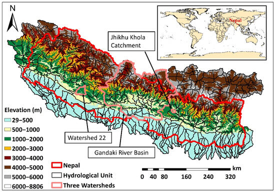
Figure 1.
A map showing a large elevation gradient and the 358 modeled watersheds in Nepal and surrounding watersheds. Watershed 22 (W22), Jhikhu Khola Catchment (JKC), and Gandaki River Basin (GRB) are used for ecohydrological model (WaSSI) evaluations.
2.2. Hydrological Model and Validation
2.2.1. Water Supply Stress Index Model (WaSSI) Description
In this study, The WaSSI model [37,49] was selected for modeling water and carbon balances at a monthly scale across the 358 watersheds with different climates and land covers in Nepal. The WaSSI model has been successfully applied in several regional and national assessments to simulate global change impacts on water balances in a variety of applications in the U.S. [49,50], Mexico and West Africa [51], Australia [52] and China [53].
The WaSSI model operates at a monthly time scale to simulate the full hydrological cycle within a watershed [37,38]. The core of the model is an empirical ET model derived from global eddy covariance data that describe total ET as a function of potential ET (PET), leaf area index (LAI), and precipitation. For this study, we used the following algorithms to estimate monthly ET:
where P is monthly precipitation (mm), LAI is the average monthly Leaf Area Index, and PET is modeled using Hamon’s temperature-based PET method. In WaSSI, ET is further constrained by soil moisture availability under extremely dry conditions.
Our initial WaSSI model testing suggested that Equation (1) above might overestimate monthly ET in regions with extremely high rainfall (i.e., >300 mm per month) during the monsoon season, so we implemented a constraint: if ET > 1.2 PET, ET is reset to Hamon PET [54,55]. Watershed monthly ET is the weight-averaged mean of ET by land cover types (deciduous, evergreen, grass, shrub, savanna, and crop).
The WaSSI model uses a conceptual snow model [56] to partition precipitation into rainfall and snowfall, and snowpack/melting is estimated using a temperature threshold. Infiltration, surface runoff, soil moisture, and baseflow processes for each land cover within each watershed are computed using algorithms of the Sacramento Soil Moisture Accounting Model (SAC-SMA).
In this study, the DEM data for Nepal with a spatial resolution of 90 m were used for the delineation of the 358 modeling watershed units using the ArcSWAT (version 2012. 10. 26, Soil and Water Assessment Tool) model (https://swat.tamu.edu/, accessed on 18 Agust 2023). The sub-watershed area threshold was set as 10 km2 for watershed delineation. International (China and India) transboundary watersheds were also accounted for in this study. Consequently, the total simulation domain area is 232,854 km2 (Figure 1).
2.2.2. WaSSI Model Validation
Previous studies have demonstrated that conventional calibrations of the model input parameters are not required because the WaSSI model was designed based on limited key ecohydrological processes and readily remote sensing data as drivers. Nonetheless, we assessed the model’s fidelity using both in situ observations (e.g., discharge data from gauging watershed) and remotely sensed ET data (Table 1). The validation was first carried out using stream discharge data from two sub-watersheds, locally designed as Jhikhu Khola catchment (JKC), Watershed 22 (W22) and one large basin (Gandaki River Basin) that covers a large portion of Nepal (Figure 1). The main reason for the selection of these three basins is that most of the basins in Nepal for which observations are available suffer from water imbalance, and only five basins have appropriate annual water balances. However, the ET/P ratios of two of these five basins exceeded the energy limits of the Budyko framework (ET > PET); therefore, only three basins (JKC, W22, and GRB) were ultimately selected for this study to evaluate the model performance at different scales. JKC is a small basin (323 km2), W22 is a medium-sized basin (13 km2), and Gandaki (36,094 km 2) is a large basin with a pronounced altitudinal gradient and climatic characteristics.

Table 1.
Datasets for hydrologic modeling and validation.
Finally, the modeled ET estimates were validated against remote sensing ET data and basin-specific ET values calculated by subtracting discharge (Q) from precipitation (P) (ET = P − Q). Performance evaluation criteria included relative model bias (%), Coefficients of Determination (r2), and slope of the regression models. The Budyko framework was also used to examine the PET/P vs. ET/P relationship [57,58] to make sure the long-term mean ET is reasonable (i.e., ET/P < 1.0).
2.3. Model Input Data
Required data to estimate Q and ET by WaSSI model include land cover type, 11 soil parameters, remotely-sensed monthly LAI (Table 1), monthly total precipitation and mean air temperature. The potential ET (PET) was derived using Hamon’s method [59], which is a function of monthly temperature and latitude [37,38,52].
2.3.1. Meteorological Data
The gridded meteorological data (i.e., precipitation and temperature) used in this study were acquired from the Third Pole Region Long Time Series High-Resolution Surface Meteorological Factor Driven Dataset (TPMFD) [60] (Table 1). The precipitation dataset is derived from high-resolution simulations based on the improved WRF model, which downscales ERA5 precipitation data by integrating simulation results and machine learning techniques. Additionally, it integrates observation data from over 9000 precipitation stations. Evaluation results indicate that its accuracy is comparable to mainstream precipitation products and reflects the spatial variation of precipitation under the complex terrain conditions of the Third Pole Region [61,62,63].
The raw data format in TPMFD is NetCDF format with a spatial resolution of 0.03° and a daily temporal resolution for the period of 1979–2022. For data preprocessing, the NetCDF format was transferred to GeoTIFF format data based on the Python (version 2.7 and 3.9) programming language to facilitate operations such as masking and statistics. The daily scale data of temperature and precipitation were scaled to a monthly scale. Then, precipitation and temperature data for each of the 358 watersheds were extracted by area-weighted average using ArcGIS (version 10.2) and Python and converted into the CSV format as model inputs.
2.3.2. Land Cover, Leaf Area Index and Soil Data
The global land use and land cover datasets produced by the European Space Agency (ESA, https://www.esa.int/ (accessed on 5 November 2024)) were used to drive WaSSI to model land cover-specific water balances. Four years of data, 2000, 2005, 2010, and 2015, were selected as inputs for each five-year land use reference. The spatial resolution of the raw data was 300 m, and the data format was in NetCDF format. In order to reduce data redundancy, the global-scale data were masked to the Lesser Himalayan region, and the spatial resolution was resampled to 1000 m to facilitate subsequent processing with the nearest neighbor method. The 36 land use types in the original remotely sensed satellite images data were reclassified into eleven land use types. These eleven land use types were Needleleaf Forest, Broadleaf Forest, Mixed Forest, Shrubland, Savanna, Cropland, Urban, Barren, Grassland, Water, Snow, and Ice. The area share of each land use type in each watershed was counted and used as a geographic information element input into the WaSSI model.
The Global Land Surface Satellite (GLASS) LAI datasets (version 3.0) were used to calculate LAI for each land use required by WaSSI. The dataset has an HDF format with a 500-m spatial resolution and an 8-day temporal resolution. Its spatial continuity is significantly better than the LAI product data from MODIS. The MODIS Tool was used to convert the data in HDF into GeoTIFF format, and then spatial statistical analysis was carried out for each geographic unit to calculate the overall LAI mean value and the corresponding LAI eigenvalues according to different land use types. The accuracy of estimated LAI dynamics was extensively validated for the study period by GLASS [64].
The soil data utilized in this study were derived from the “A priori global 250m parameter dataset for the SAC-SMA model” [65]. This dataset includes 11 essential soil parameters required for SAC-SMA modeling. It was derived from the Global 250 m Soil Hydraulic Properties dataset [66], integrating data from SoilGrids 250m 2.0 (https://soilgrids.org (accessed on 1 May 2020)) and the Copernicus Climate Change Service (C3S) Global Land Cover dataset (2020, 300-m resolution) (https://cds.climate.copernicus.eu/datasets/satellite-land-cover?tab=overview (accessed on 19 April 2024)). Full details related to the development of this dataset are described in the related technical reports [59].
2.4. Model Validation Data
2.4.1. Observed Streamflow Data for Calculating ET and Model Validation at a Watershed Scale
The daily discharge (Q) dataset was used to validate the WaSSI model at the watershed level. Our previous study found that only five watersheds among the 12 watersheds initially selected were qualified for ET model validation purposes due to potential issues of water imbalances as judged by the Budyko framework (unpublished data). We selected JKC and W22 catchments, and another large basin (Gandaki River basin, GRB) for model assessment. Watershed actual ET was calculated based on water balance () on the annual scale.
At the annual scale, the change in annual soil storage () is small and assumed to be negligible.
2.4.2. National Remote Sensing Based ET Products
We used four ET products to assess WaSSI model performance at the national scale including the Operational Simplified Surface Energy Balance (SSEBop) model, ETMonitor, Proportionality hypothesis-based surface Energy–Water balance model (PEW), and FLUXCOM (Table 1). SSEBop ET product provided ET at monthly and 1-km resolution [67]. SSEBop ET estimates compared reasonably well with monthly eddy covariance ET data explaining 64% of the observed variability across diverse ecosystems in the continental U.S. [67]. ETMonitor is a distributed ET model that integrates land surface characteristics [68]. The model considers evaporation, transpiration, or sublimation from soil, vegetation, water bodies, and snow within the same pixel. The model considers three parts of the energy balance, the radiation processes of vegetation and soil, the ecophysiological processes of vegetation, and the water balance processes. PEW [69] is based on the generalized proportionality hypothesis on water balance [70]. The PEW product incorporates precipitation data in its model construction, which is one of its unique features compared to other remote sensing-based ET products. The FLUXCOM data stream is produced using machine learning to merge eddy flux measurements from the FLUXNET eddy covariance measurement network with remote sensing and meteorological data to estimate net radiation, latent and sensible heat and their uncertainties [71]. The resulting FLUXCOM database comprises 147 global gridded products in two setups: 0.0833° resolution using MODIS remote sensing data (RS) and 0.5° resolution using remote sensing and meteorological data (RS + METEO).
3. Results
3.1. Model Validations at Multiple Scales
3.1.1. Validating the WaSSI Model with Discharge and ET
The monthly discharge simulated by the WaSSI model performed reasonably when compared against observed flow data from the local gauging station in JKC (Figure 2a). On a monthly scale, the correlation coefficient between the observed and simulated runoff values was 0.85, with an r2 of 0.7 (Figure 2a). The deviation between the two was 5.8 ± 40.8 mm month−1, with a relative error of 14.7%. However, the model tends to underestimate runoff during the dry season (December–February) while exhibiting a large positive bias (an average of 51.5 mm) during the monsoon season (June–September). The simulated results of the WaSSI are generally lower by 19.7 mm in the dry season (Figure 2b).
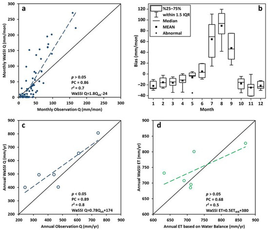
Figure 2.
Annual and monthly scatter plot between simulation and observed discharge (Q) and evapotranspiration (ET) for the JKC watershed during 2000–2005. (a) Monthly WaSSI Q vs. monthly observed Q, (b) Monthly bias between WaSSI Q and observed Q, (c) Annual WaSSI Q vs. annual observed Q, and (d) Annual WaSSI ET vs. annual ET-based water balance (ETwb). PC is Pearson’s correlation coefficient. The black solid line represents the 1:1 line while the dashed solid line denotes the fitted line.
On an annual scale, the WaSSI simulations for Q show a better correlation with the observations (Figure 2c). During the period 2000–2005, the mean deviation was 69.5 ± 83.4 mm yr−1, with a relative error of 14.7%. The correlation between the simulated and observed Q is significantly higher than at the monthly scale with a Pearson’s correlation coefficient of 0.89 and an r2 of 0.8 (p < 0.05) (Figure 2c). Simulated annual ET by WaSSI compared well with ET calculated using the water balance method () (Figure 2d) with an r2 of 0.5, and the Pearson’s correlation coefficient is 0.68. The average bias between the two on the annual scale was small, with the simulated values being lower than ETWB by 19 ± 59 mm yr−1, with a relative error of 2.6%.
Overall, the WaSSI model captured the temporal variations of both ET and Q in response to rainfall patterns at the monthly and annual scales (Figure 2). The WaSSI model performed better than the remote sensing product ETMonitor (Table 2). The small model bias percentage and high regression values at the annual scale indicate that WaSSI can satisfactorily simulate long-term temporal variability of the Q and ET.
Table 2.
Mean annual comparison between WaSSI Q vs. observed Q (Qobs), WaSSI ET vs. P − Qobs (ETWB), and WaSSI ET vs. ETMonitor product from 2001 to 2005 for the JKC watershed.
3.1.2. Model Validation on ET Using Remote Sensing Products at Multiple Scales
We used the four remote sensing products (Table 1) to assess WaSSI’s ability to model ET at different spatial and temporal scales. The spatial scales include two small catchments (JKC and W22), a large basin (Gandaki River Basin, GRB), and the whole of Nepal. Our previous preliminary study has found that the ETMonitor remote sensing products are superior among multiple remote sensing ET products evaluated for JKC [65]. Therefore, we adopted the ETMonitor product for model validation at the monthly and annual scales. On the monthly scale, we found a high Pearson’s correlation coefficient of 0.8 (p < 0.05) and an r2 of 0.63 (Figure 3a,b). The average difference between the two on the monthly scale was −4.5 ± 22.3 mm mon−1, with a small relative error of −6.9%. The difference between the two was small in the dry season (December–February). However, in March–June, WaSSI ET was much lower than ETMonitor ET, with a mean deviation of −24.5 mm mon−1, whereas in July–September WaSSI ET was higher, with a mean deviation of 15.9 mm mon−1 (Figure 3b).
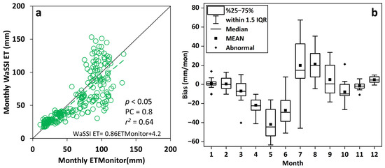
Figure 3.
A comparison between modeled monthly ET by the WaSSI model and estimates by ETMonitor for the JKC watershed during 2000–2020. (a) Scatter plot, and (b) Monthly differences (WaSSI ET minus ETMonitor ET). In (a), the black solid line represents the 1:1 line, while the dashed solid line denotes the fitted line.
Large discrepancies were found when comparing annual ET variations with the four remote sensing products (ETMonitor, SSEBop, and PEW, FLUXCOM) and ETwb for the two small watersheds (JKC and W22) and one large basin (GRB) (Figure 4). Harmon-PET data were also plotted and compared with ET products to assess the quality of these products. We found that both ETMonitor and WaSSI ET showed an increasing trend in the JKC between 2000 and 2020, with rates of 1.0 mm yr−1 for WaSSI ET and 3.2 mm yr−1 for ETMonitor. Overall, annual WaSSI ET was −53.4 ± 69 mm yr−1 lower than the ETMonitor, with a small average relative error of −6.9%. It is noteworthy that FLUXCOM’s ET estimates were much higher than other ET estimates in JKC, even higher than Hamon-PET (Figure 4a). In W22, the ETMonitor and WaSSI ET simulations were closely aligned (Figure 4b). In the large GRB, the WaSSI ET simulations were close to the PEW and SSEBop ET estimates (Figure 4c).
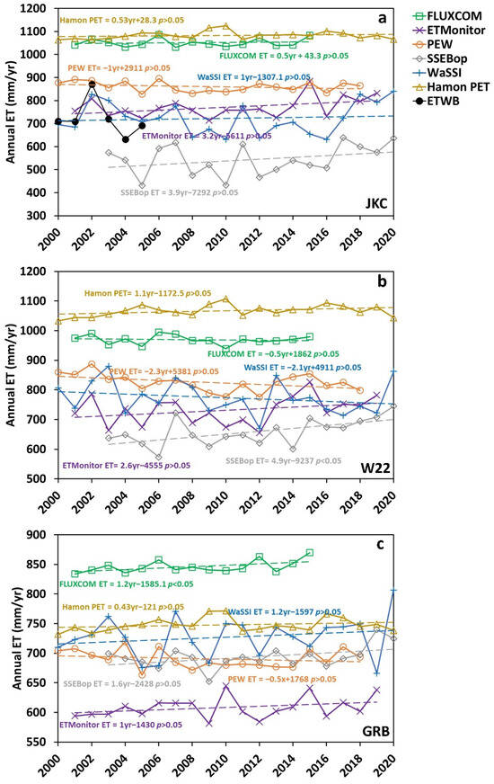
Figure 4.
Annual ET comparisons among FLUXCOM ET, remote sensing products (ETMonitor, SSEBop ET, and PEW ET), water balance-based ET (ETwb), WaSSI ET, and Harmon-PET from 2000 to 2020 in three watersheds (a) Jhikhu Khola catchment (JKC), (b) Watershed 22 (W22), and (c) Gandaki River Basin (GRB).
Comparisons of multi-year mean WaSSI ET and other products at the national level show that WaSSI performed well overall in Nepal, with r2 of 0.85 for ETMonitor, 0.85 for FLUXCOM, 0.92 for PEW, and 0.73 for SSEBop (Figure 5). Among the four remote sensing-based ET products, ETMonitor showed the strongest agreement with WaSSI, with a mean deviation value of 29 ± 135 mm and a relative deviation of 4.6% (Figure 5a). However, spatially, WaSSI ET simulation was found to be lower than ETMonitor in the high mountainous areas of northern Nepal (cold regions), with an average deviation of about 150 mm. In contrast, WaSSI ET was higher by more than 150 mm in the mid-mountainous regions (wet and warm regions) and 0–200 mm in other regions (Figure 5a).
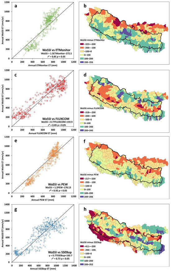
Figure 5.
WaSSI model validations for mean annual ET during 2000–2020. The left panel shows scatter plots comparing WaSSI ET with four remote sensing-based ET products, while the right panel presents difference maps (WaSSI ET minus ET products) to illustrate the magnitude and distribution of spatial similarities between the different datasets across Nepal. (a) WaSSI vs. ETMonitor, (b) bias pattern between WaSSI and ETMonitor, (c) WaSSI vs. FLUXCOM, (d) bias pattern between WaSSI and FLUXCOM, (e) WaSSI vs. PEW, (f) bias pattern between WaSSI and PEW, (g) WaSSI vs. SSEBop, and (h) bias pattern between WaSSI and SSEBop. In (a,c,e,g), the black solid line represents the 1:1 line, while the dashed solid line denotes the fitted line.
Similarly, compared with PEW, the WaSSI model mostly overestimated ET in the mid-mountainous regions of Nepal while generally underestimating it in the high mountainous areas of northern Nepal (Figure 5c). On the contrary, compared with FLUXCOM, the WaSSI model mostly overestimated ET in the high mountainous regions of Nepal while underestimating it in the mid-mountainous areas (Figure 5b). Compared with SSEBop, the WaSSI model generally overestimated ET across Nepal, except in the southwestern region (Figure 5d).
3.2. Spatiotemporal Patterns of Water Balances at the National Scale
3.2.1. Spatial Distributions of Hydrological Variables
Both mean watershed ET and Q varied dramatically in Nepal from 2000–2020 (Figure 6). The mean annual ET values across Nepal ranged from 150 to 1100 mm yr−1 and showed a decreasing distribution with altitude from the south to the north (Figure 6a). The south-central plains in the central GRB have the highest ET (more than 1000 mm yr−1) corresponding to a region with high P (Figure 6c) and PET (Figure 6d) followed by the southeastern region, and the cool high-altitude northwestern region where ET < 400 mm yr−1. The watershed with a high Q in Nepal is also found in the central GRB with the highest P (Figure 6b,c), where some of its sub-watersheds have an annual Q of more than 1600 mm yr−1.
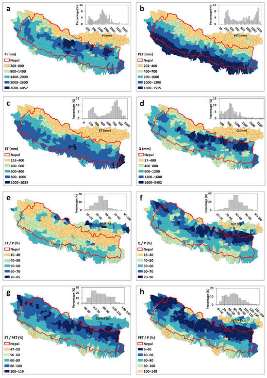
Figure 6.
WaSSI modeled mean (2000–2020) annual water balances as quantified by actual precipitation (P), evapotranspiration (ET), water yield (Q) and other indicators across 385 watersheds in Nepal. (a) Precipitation (P, mm yr−1), (b) Potential ET (PET, mm yr−1), (c) ET (mm yr−1), (d) Q (mm yr−1), (e) Ratios between ET and P (%), (f) Runoff coefficients (Q/P, %), (g) Ratios between ET and PET (%), and (h) Ratios between PET and P (%). The figure inserts in a–d are frequency distributions.
The ET/P ratio reflects the efficiency of water use or precipitation partitioning as ‘green water’, while the Q/P ratio (runoff coefficient) indicates the proportion of precipitation converted to runoff or ‘blue water’. Across Nepal, ET/P ratios decrease with altitude from south to north, whereas Q/P ratios show the opposite trend (Figure 6e,f). Generally, areas with high ET/P ratios in southern Nepal imply that water resources are more fully utilized or precipitation is relatively deficient. In contrast, areas with low ET/P ratios in mid- and high mountain regions indicate precipitation less fully utilized (Figure 6c) as ‘Green water’ and more precipitation is partitioned as ‘blue water’. Areas with a high Q/P ratio in the mid- and high mountainous regions of Nepal have low PET and steep slopes but low P, resulting in more precipitation being converted to runoff. In contrast, areas with low Q/P ratio are found in the northern Terai Plain with gentle slopes where high ET and moderate P are present.
3.2.2. WaSSI Result Summary on Budyko Framework
The WaSSI modeling results are further summarized using the Budyko energy and water balance framework, which provides a long-term picture of the hydrometeorological regime and how evapotranspiration efficiency (EP/P) responds to variation of the climatic regime as quantified by the dryness index (PET/P) (Figure 7). Overall, the simulated mean ET/P data follow the general Budyko curve, developed using one of the commonly used Fu [58] models (Figure 7). The majority of the 358 watersheds are considered not water stressed (PET/P < is 1.0)—precipitation can meet the potential water evaporative demand at the annual scale. The majority of the watersheds have ET/P ratios less than 0.6 or Q/P ratios (or 1 − ET/P) higher than 0.4. However, ET/P values for some watersheds that receive precipitation less than 800 mm in the high mountains (Figure 6e) deviate from the general pattern. A close examination reveals that the LAI values for these watersheds are uncharacteristically high, resulting in over-prediction of ET by the WaSSI model (Figure 6e).
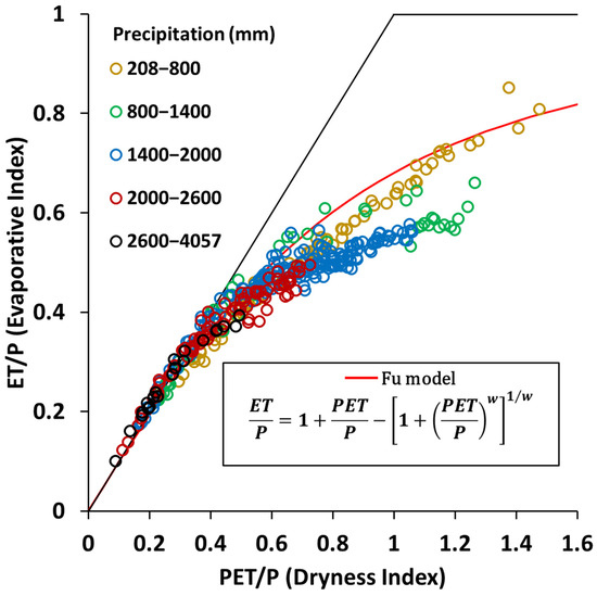
Figure 7.
The Budyko framework shows relations between the mean annual Evaporative Index (ET/P) vs. Dryness Index (DI = PET/P). The dashed line represents the Fu model [58] with a parameter w = 2.5. The data points are presented in color by annual precipitation (mm) acquired from the Third Pole Region Long Time Series High-Resolution Surface Meteorological Factor Driven Dataset (TPMFD).
3.2.3. Temporal Trend of Annual Water Balance
A nonparametric trend testing (Mann–Kendall test, M-K test) method [72,73] was employed for trend analysis across Nepal. Based on the M-K test results, P shows decreasing trends in western and southern regions while exhibiting increasing patterns in certain northern basins (Figure 8a). M-K result of water yield (Q) demonstrates no significant changes across most areas, though declines are observed in specific basins of the western, southern, and southeastern regions (Figure 8b). In contrast, some high-altitude basins in northern areas reveal upward trends in Q. Evapotranspiration remains largely stable throughout most territories, with observable increases primarily concentrated in select northern watersheds (Figure 8c).
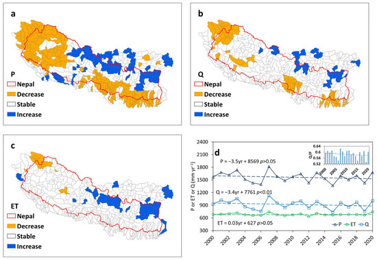
Figure 8.
Simulated water balance across 385 watersheds in Nepal during 2000–2020. (a) M-K trend pattern of precipitation (P), (b) M-K trend pattern of runoff (Q), (c) M-K trend pattern of evapotranspiration (ET), (d) P, Q, and ET are area-weighted annual mean precipitation (mm yr−1), water yield (mm yr−1), and actual evapotranspiration (mm yr−1), respectively. The insert figure shows the trend of the mean annual runoff coefficient (Q/P).
The WaSSI water balance simulation results showed that, during the past 21 years (2000–2020), the long-term mean annual ET was 684 mm, nearly half the mean precipitation of 1567 mm. Mean annual stream flow slightly decreased from 903 mm to 853 mm from period 1 (2000–2011) to period 2 (2012–2020) (Figure 8d). This represents a slight decrease in the runoff coefficient (Q/P) from 0.57 to 0.55 (insert in Figure 8d). The trend of annual stream flow was influenced heavily by the year 2007 with a large precipitation of 1817 mm. In the meantime, annual ET was stable with an average of 684 mm for the two periods. Our results show that precipitation dominated the water balances in Nepal, and the balance between ET and precipitation explained the annual dynamics of water yield.
4. Discussion
This regional modeling study represents the most complete, explicit mapping of water balances (P, Q, ET) that considers the key biophysical controls to ET in 358 watersheds across Nepal and surrounding areas. Different from previous studies that focus on individual basins [6,44] or sub-regions at the national scale [38] in Nepal, this work uses an integrated watershed modeling approach that provides a ‘wall-to-wall’ modeling of the monthly water balances of intermediate-size watersheds over a two-decade period. The modeled water balance spatial patterns reflect the dominant controls of a monsoon climate and elevation/topography gradient in Nepal. The watersheds that yield most of the water are those with an elevation in the 2000–3000 m zone, not in the mountains with the highest elevations (>3000 m)—the perceived ‘Water Tower’. This finding is consistent with the report that most of the streamflow in the Himalaya regions is from the middle mountains where precipitation is highest and the Tibetan Plateau is not the ‘Water Tower’ [74]. Additionally, recent research has revealed that glacial meltwater from the Tibetan Plateau plays a limited role in sustaining downstream water resources, as precipitation constitutes the dominant contributor to runoff [75,76]. This conclusion remains to be our tentative hypothesis at this stage, definitive confirmation would require additional field studies including establishing monitoring stations in high-altitude regions to validate these findings.
4.1. Success and Uncertainty of the WaSSI Model and Remote Sensing ET Products
It appears that the WaSSI model that was developed outside of the study region [36,37] provides a reasonable estimate of water balances in Nepal when compared to a small watershed site. The ET estimates by WaSSI also compare favorably when compared to remote sensing products at the national and annual levels. In addition, the simulated mean ET/P-PET/P relations follow the Budyko framework reasonably well for most watersheds (Figure 7), providing confidence that WaSSI as a monthly scale model captures the general water balances. However, WaSSI overestimated annual ET in regions with high ET where precipitation is extremely high in the middle mountain regions, such as the Gandaki River Basin. The modeled annual ET values for the JKC watershed generally exceed 600 mm with a long-term mean of 700 mm. These estimates contrast with findings by a one-year (2010–2011) field study that reports annual ET of 250 mm, 524 mm, and 577 mm for degraded pasture, natural forest, and pine forest, respectively [29]. We consider these measured ET rates as the low-end values for the central mountain regions [15,30].
Discrepancies between modeled and estimated Q and ET at the watershed and regional levels may come from several key sources. These include issues with ET model algorithms, model parameters [40], and spatial input data (e.g., leaf areas index and land cover types, soil characterizations) that drive the model. For example, most of the existing meteorological stations are found in low-altitude areas, leading to underestimation of precipitation and overestimation of air temperature. It is not uncommon for monitored streamflow to exceed precipitation as found in our previous study. Also, the remote sensing-based ET products and the ET estimates using watershed hydrological balances have uncertainty.
In this study, the empirical formulas for estimating ET and PET by WaSSI are constructed from North America and other regions. Despite making a minor modification to ET algorithms, the ET model likely still has deficiency in accounting for the local climatic and terrain and vegetation (i.e., forest communities) conditions in the lower Himalayas. For example, distinguishing between sunny and shady slopes and accounting for fog effects on energy availability (e.g., solar radiation) are important for accurately estimating ET [77]. The size of water bodies can also influence terrestrial energy balance to some extent [78]. Significant vertical climatic variations also require refinement of climate data inputs, especially in precipitation. Furthermore, the ET model used in WaSSI also has its inherent limitations that balance input data needs and model accuracy [37,79]: (1) The model might be biased when only air temperature is used for estimating PET in lieu of radiation, humidity, and wind speed data because plant stomatal conductance and transpiration are sensitive to radiation and vapor pressure deficit, and (2) The WaSSI model uses LAI as the only vegetation structure variable to estimate total ET, not each of the ET components. Other biophysical processes such as canopy interception, hydraulic redistribution, stomatal regulations of water uptake, and soil preferential flows are not explicitly modeled, but can be important in the study region.
Our study found that remote sensing products, SSEBop, PEW, ETmonitor, and FLUXCOM, have large uncertainty in characterizing ET patterns at both individual watersheds and across Nepal (Figure 5 and Figure 6). Although it remains difficult to rank the accuracy of each product since ground measurements are lacking, we could narrow down the general applicability of these ET products by integrating them with WaSSI ET results. For example, FLUXCOM obviously overestimates ET (by more than 300 mm) at the JCK watershed (Figure 5a) because annual actual ET should rarely exceed PET. Therefore, although the FLUXCOM data developed using global eddy flux measurements have the advantages of high spatial and temporal resolution, fusion of multiple data sources, and broad applicability in complex terrain, they have limitations in Nepal perhaps due to the model’s empirical nature and input data limitation. Annual ET estimates by SSEBop and PEW are similar for the GRB case (Figure 5c) but not for the other two watersheds (JKC and W22) (Figure 5a,b). Both datasets show more than 100 mm higher than the ETmonitor estimates and 50 mm lower than WaSSI ET for the GRB case (Figure 5c). SSEBop ET values compared more than 200 mm lower than other products (ETMonitor, PEW) for both JKC and W22 cases (Figure 5a,b) with annual ET of less than 600 mm, which is considered unrealistic for a subtropic region. SEEBop ET modeling is based on the principle of energy balance and uses the ratio of surface temperature to reference temperature [67], and the choices of PET calculation methods have large influences on the resulting ET accuracy. So, SSEBop products likely have limitations due to topographic effects, cloud cover, and parameterization schemes to accommodate the high spatial heterogeneity of surface temperature and PET algorithms that should reflect landcover characteristics. The PEW ET estimates generally fall in the middle of the ET products examined in this study (Figure 5b,c), but PEW is considered somewhat high for the JKC watershed since the values are almost as high as PET (Figure 5a). Although the PEW ET products are based on the Priestley Taylor–Jet Propulsion Laboratory (PT-JPL) algorithm [80], there is no guarantee of model accuracy, which largely depends on the reliability of remote sensing data for land characteristics and model parameterization, as both are challenging in Nepal. The ETmonitor products are based on multi-source data fusion, combining remote sensing, meteorological monitoring, and ground observation data, and have been recognized to be the most reliable overall in our previous assessment in Nepal (unpublished data) and this study (Figure 5). However, the lack of ground observation data makes it difficult to make a broad statement on the model’s accuracy.
On seasonal scales, the WaSSI simulation results exhibit certain discrepancies compared to actual observations and product data. First, in comparison with monthly observed Q, the most pronounced difference occurs during the rainy season (June to September). During this period, runoff estimates are systematically higher, likely due to overestimated precipitation inputs in the model, as rainy-season runoff variations are primarily precipitation-controlled and ET modeling errors should have little contribution to the overall model bias. Seasonal-scale ET results show deviations from the ETMonitor product, mainly characterized by lower estimates in the pre-monsoon season and higher estimates during the monsoon season. We attribute these differences to several key factors. Energy-wise, winter temperatures are relatively low, leading to closer agreement between the two ET simulations. However, as temperatures gradually rise during the pre-monsoon period, discrepancies emerge. ETMonitor uses net radiation flux as its energy input, whereas WaSSI relies on temperature-based PET, resulting in divergent energy component estimations during the pre-monsoon season when precipitation remains limited ETMonitor’s energy input estimates may exceed those of WaSSI under these conditions. Compared to the Penman–Monteith [81] equation recommended by FAO-56 or the Priestley–Taylor [82] model, the Hamon PET model has a simpler structure and requires only air temperature data as input. Notably, air temperature data are the easiest and highest-quality meteorological variable to obtain in this data-poor region. Furthermore, since ETMonitor ET calculations do not involve precipitation, while WaSSI incorporates precipitation inputs, the influence of precipitation on evapotranspiration discrepancies may become more pronounced during the monsoon season.
The variability in data inputs is another key factor contributing to uncertainty in model outcomes. Different models require varying types of input data, and even distinct modeling products often demand slightly different input parameters. These discrepancies naturally lead to variations in output results. In Nepal’s case, where data scarcity remains a persistent challenge, this limitation becomes particularly pronounced—essentially acting as a multiplier that amplifies differences between simulation results from various models. It is like trying to solve the same puzzle with different sets of missing pieces; each model inevitably fills the gaps differently based on its unique data requirements and available information.
In our linear regression model analysis for WaSSI model validation for the JKC basin and cross-comparison with various remote sensing products, we observed that the scatterplot’s linear fit failed the Durbin–Watson test, suggesting potential autocorrelation among samples. However, annual-scale ET and Q simulations from the WaSSI model successfully passed multiple diagnostic checks including the Durbin–Watson autocorrelation test, White test, and Studentized Residuals outlier assessment, although they did not satisfy the normality requirement in the Q-Q plot evaluations.
Spatially, Mann–Kendall trend analysis revealed declining P and Q patterns across most regions, aligning with overall linear trend observations. Meanwhile, ET maintained stable trends in most areas, consistent with its aggregated behavior. Our conceptual model based on the Budyko framework demonstrated close alignment with Fu curve predictions under this theoretical structure. While data limitations constrained long-term temporal validation, the convergence of evidence from multiple analytical perspectives—including trend consistency across scales, diagnostic test outcomes, and theoretical framework compatibility collectively indicates that WaSSI model outputs show enhanced reliability when compared to alternative ET products.
4.2. Implications to Water Resources Under a Changing Environment
This national water balance modeling study shows that most of the watersheds in Nepal are dominated by an ‘energy-limited’ (P > PET) hydrology due to high precipitation in the summer months (May–September), as they are influenced by a monsoon climate. However, the seasonable distribution of precipitation and water yield is very uneven in Nepal, resulting in well-known extreme hydrologic hazards such as floods and erosion in the wet season and water shortages in the dry season [83,84]. Although this modeling study did not detect an overall increase in ET for the study period, there is an expectation that water loss through ET will increase in some basins in Nepal due to land ‘greening up’ and/or global warming [33], which is especially pronounced at higher altitudes. Glaciers retreat due to global warming and are elevate river flow in high-elevation watersheds [3]. Climate change is hydrologic change [11]. Climate change is projected to have a significant impact on the water balances in the Hindu Kush Himalayas, including Nepal [85]. Most of the studies show a decreasing trend in annual precipitation in Nepal over the past decades, but there are significant regional and seasonal differences. For example, precipitation decreased in the western mountains and increased in the east, and there has been an increase in the frequency and intensity of extreme precipitation events [5], leading to more severe flooding and landslides. Reduced precipitation has directly led to a decrease in water production, especially in the western mountainous regions, resulting in a decline in spring water flow, a major water source for rural communities in the Himalaya region [4,86].
This study focuses on water resources and how the WaSSI can be used to map the temporal and spatial distribution. The WaSSI model has the capacity to estimate carbon balances and this function needs to be evaluated to understand carbon and water tradeoff when it comes to ecosystem service quantifications. The WaSSI model mainly looks at how climate and vegetation affect water and carbon systems under natural conditions, but it does not fully account for human activities. This model deficiency could impact how we assess water management in regions with large agricultural farming activities downstream with irrigation in the south. Future studies should combine economic models with population, social, and economic data, creating a water–society–economy model that helps developing countries plan their water use more holistically.
5. Conclusions
This study developed a national water balance dataset for Nepal by integrating hydrometeorological monitoring data, land use and land cover data, and watershed information with an ecohydrological model. The study indicates that the WaSSI model outperforms most global remote sensing products in capturing ET dynamics at the watershed and national levels. It appears that a combination of remotely sensed data, ground-based observations, and hydrologic models is effective in estimating water balances for data-poor regions by identifying potential uncertainties in each hydrologic flux.
Future water balance studies should focus on improving the research capacity of measuring ET of forests and croplands, the two dominant land uses in Nepal, to improve algorithms of remote sensing-based ET models that capture the spatial heterogeny of terrain, climate and vegetation. Ground-based monitoring of meteorological variables and streamflow in small watersheds (<100 km2) facilitates the development of accurate watershed water balances. These hydrological budgets are particularly valuable for refining modeling tools, which can be broadly applied in watershed management decision-making to mitigate water security risks and enhance resilience against rapidly evolving environmental pressures, notably climate change and land-use transitions.
Author Contributions
Conceptualization, G.S. and L.H.; Data curation, K.J. and R.T.; Formal analysis, K.J., N.L. and R.T.; Funding acquisition, G.S. and L.H.; Methodology, K.J., N.L. and R.T.; Project administration, L.H.; Software, K.J., N.L. and G.S.; Supervision, G.S. and L.H.; Validation, K.J. and N.L.; Writing—original draft, K.J., N.L., G.S. and L.H.; Writing—review and editing, K.J., N.L., G.S. and L.H. All authors have read and agreed to the published version of the manuscript.
Funding
This research was funded by the National Natural Science Foundation of China, grant numbers 42061144004 and 41877151 (principal investigator: Lu Hao, NUIST). Partial support is also from the Southern Research Station USDA Forest Service.
Data Availability Statement
The data that support the findings of this study are available upon reasonable request from the authors.
Conflicts of Interest
The authors declare that they have no known competing financial interests or personal relationships that could have appeared to influence the work reported in this paper.
References
- Bruijnzeel, L.; Sun, G.; Zhang, J.; Tiwari, K.; Hao, L. Forests, Water, and Livelihoods in the Lesser Himalaya. Eos. 2024. Available online: https://research.fs.usda.gov/treesearch/68169 (accessed on 15 May 2024).
- Xu, J.; Grumbine, R.E.; Shrestha, A.; Eriksson, M.; Yang, X.; Wang, Y.U.N.; Wilkes, A. The melting Himalayas: Cascading effects of climate change on water, biodiversity, and livelihoods. Conserv. Biol. 2009, 23, 520–530. [Google Scholar] [CrossRef] [PubMed]
- Chaulagain, N.P. Impacts of Climate Change on Water Resources of Nepal: The Physical and Socioeconomic Dimensions. Ph.D. Thesis, Flensburg University, Flensburg, Schleswig-Holstein, Germany, 2007. [Google Scholar]
- Pandit, A.; Batelaan, O.; Pandey, V.P.; Adhikari, S. Depleting spring sources in the Himalayas: Environmental drivers or just perception? J. Hydrol. Reg. Stud. 2024, 53, 101752. [Google Scholar] [CrossRef]
- Luo, Y.; Wang, L.; Hu, C.; Hao, L.; Sun, G. Changing extreme precipitation patterns in Nepal over 1971–2015. Earth Space Sci. 2024, 11, e2024EA003563. [Google Scholar] [CrossRef]
- Acharya, S.; Hori, T.; Karki, S. Assessing the spatio-temporal impact of landuse landcover change on water yield dynamics of rapidly urbanizing Kathmandu valley watershed of Nepal. J. Hydrol. Reg. Stud. 2023, 50, 101562. [Google Scholar] [CrossRef]
- Poudel, N.; Shaw, R. Challenges of Urban Water Security and Drivers of Water Scarcity in Kathmandu Valley, Nepal. Urban Sci. 2025, 9, 54. [Google Scholar] [CrossRef]
- United Nation-Habitat. Cities and Climate Action: World Cities Report 2024. Available online: https://unhabitat.org/ (accessed on 12 May 2025).
- Kulkarni, H.; Desai, J.; Siddique, M.I. Rejuvenation of springs in the Himalayan Region. In Water, Climate Change, and Sustainability, 1st ed.; Pandey, V.P., Shrestha, S., Wiberg, D., Eds.; John Wiley & Sons, Inc.: Hoboken, NJ, USA, 2021; pp. 97–107. [Google Scholar]
- Vose, J.M.; Sun, G.; Ford, C.R.; Bredemeier, M.; Otsuki, K.; Wei, X.; Zhang, Z.; Zhang, L. Forest ecohydrological research in the 21st century: What are the critical needs? Ecohydrology 2011, 4, 146–158. [Google Scholar] [CrossRef]
- Sun, G.; Tiwari, K.R.; Hao, L.; Amatya, D.; Liu, N.; Song, C. Climate change and forest hydrology in future forests. In Future Forests Mitigation and Adaptation to Climate Change; Elsevier Inc.: Amsterdam, The Netherlands, 2024; Chapter 6; pp. 95–124. [Google Scholar]
- Sun, G.; Hallema, D.; Asbjornsen, H. Ecohydrological processes and ecosystem services in the Anthropocene: A review. Ecol. Process. 2017, 6, 35. [Google Scholar] [CrossRef]
- Badu, M.; Nuberg, I.; Ghimire, C.P.; Bajracharya, R.M.; Meyer, W.S. Negative trade-offs between community forest use and hydrological benefits in the forested catchments of Nepal’s mid-hills. Mt. Res. Dev. 2019, 39, R22. [Google Scholar] [CrossRef]
- Thapa, B.R.; Ishidaira, H.; Pandey, V.P.; Shakya, N.M. A multi-model approach for analyzing water balance dynamics in Kathmandu Valley, Nepal. J. Hydrol. Reg. Stud. 2017, 9, 149–162. [Google Scholar] [CrossRef]
- Talchabhadel, R.; Chhetri, R. Evaluation of long-term changes in water balances in the Nepal Himalayas. Theor. Appl. Climatol. 2024, 155, 439–450. [Google Scholar] [CrossRef]
- Bastola, S.; Seong, Y.J.; Lee, S.H.; Jung, Y. Water yield estimation of the Bagmati basin of Nepal using GIS based InVEST model. J. Korea Water Resour. Assoc. 2019, 52, 637–645. [Google Scholar]
- Bharati, L.; Gurung, P.; Jayakody, P.; Smakhtin, V.; Bhattarai, U. The projected impact of climate change on water availability and development in the Koshi Basin, Nepal. Mt. Res. Dev. 2014, 34, 118–130. [Google Scholar] [CrossRef]
- Budhathoki, B.R.; Adhikari, T.R.; Shrestha, S.; Awasthi, R.P. Application of hydrological model to simulate streamflow contribution on water balance in Himalaya river basin, Nepal. Front. Earth Sci. 2023, 11, 1128959. [Google Scholar] [CrossRef]
- Dhami, B.; Himanshu, S.K.; Pandey, A.; Gautam, A.K. Evaluation of the SWAT model for water balance study of a mountainous snowfed river basin of Nepal. Environ. Earth Sci. 2018, 77, 21. [Google Scholar] [CrossRef]
- Baniya, B.; Tang, Q.; Adhikari, T.R.; Zhao, G.; Haile, G.G.; Sigdel, M.; He, L. Climate change induced Melamchi extreme flood and environment implication in central Himalaya of Nepal. Nat. Hazards 2024, 120, 11009–11029. [Google Scholar] [CrossRef]
- Pradhan, A.M.S.; Silwal, G.; Shrestha, S.; Huynh, T.C.; Dawadi, S. Can a Spatially Distributed Hydrological Model Effectively Analyze Hydrological Processes in the Nepal Himalaya River Basin? Environ. Model. Assess. 2024, 29, 1037–1058. [Google Scholar] [CrossRef]
- Nepal, S.; Krause, P.; Flügel, W.A.; Fink, M.; Fischer, C. Understanding the hydrological system dynamics of a glaciated alpine catchment in the Himalayan region using the J2000 hydrological model. Hydrol. Process. 2014, 28, 1329–1344. [Google Scholar] [CrossRef]
- Shrestha, S.; Nepal, S. Water balance assessment under different glacier coverage scenarios in the Hunza Basin. Water 2019, 11, 1124. [Google Scholar] [CrossRef]
- Zhang, Y.; Kong, D.; Gan, R.; Chiew, F.H.; McVicar, T.R.; Zhang, Q.; Yang, Y. Coupled estimation of 500 m and 8-day resolution global evapotranspiration and gross primary production in 2002–2017. Remote Sens. Environ. 2019, 222, 165–182. [Google Scholar] [CrossRef]
- Bhattarai, N.; Wagle, P. Recent advances in remote sensing of evapotranspiration. Remote Sens. 2021, 13, 4260. [Google Scholar] [CrossRef]
- Sun, G.; Wei, X.; Hao, L.; Sanchis, M.G.; Hou, Y.; Yousefpour, R.; Tang, R.; Zhang, Z. Forest hydrology modeling tools for watershed management: A review. For. Ecol. Manag. 2023, 530, 120755. [Google Scholar] [CrossRef]
- Zhang, J.; Kong, D.; Li, J.; Qiu, J.; Zhang, Y.; Gu, X.; Guo, M. Comparison and integration of hydrological models and machine learning models in global monthly streamflow simulation. J. Hydrol. 2025, 650, 132549. [Google Scholar] [CrossRef]
- Yi, K.; Senay, G.B.; Fisher, J.B.; Wang, L.; Suvočarev, K.; Chu, H.; Moore, G.W.; Novick, K.A.; Barnes, M.L.; Keenan, T.F.; et al. Challenges and future directions in quantifying terrestrial evapotranspiration. Water Resour. Res. 2024, 60, e2024WR037622. [Google Scholar] [CrossRef]
- Ghimire, C.P.; Bruijnzeel, L.A.; Lubczynski, M.W.; Bonell, M. Negative trade-off between changes in vegetation water use and infiltration recovery after reforesting degraded pasture land in the Nepalese Lesser Himalaya. Hydrol. Earth Syst. Sci. 2014, 18, 4933–4949. [Google Scholar] [CrossRef]
- Srinet, R.; Nandy, S.; Watham, T.; Padalia, H.; Patel, N.R.; Chauhan, P. Measuring evapotranspiration by eddy covariance method and understanding its biophysical controls in moist deciduous forest of northwest Himalayan foothills of India. Trop. Ecol. 2022, 63, 387–397. [Google Scholar] [CrossRef]
- Deb Burman, P.K.D.; Launiainen, S.; Mukherjee, S.; Chakraborty, S.; Gogoi, N.; Murkute, C.; Lohani, P.; Sarma, D.; Kumar, K. Ecosystem-atmosphere carbon and water exchanges of subtropical evergreen and deciduous forests in India. For. Ecol. Manag. 2021, 495, 119371. [Google Scholar] [CrossRef]
- Deb Burman, P.K.; Sarma, D.; Morrison, R.; Karipot, A.; Chakraborty, S. Seasonal variation of evapotranspiration and its effect on the surface energy budget closure at a tropical forest over north-east India. J. Earth Syst. Sci. 2019, 128, 127. [Google Scholar] [CrossRef]
- Dorji, U.; Olesen, J.E.; Seidenkrantz, M.S. Water balance in the complex mountainous terrain of Bhutan and linkages to land use. J. Hydrol. Reg. Stud. 2016, 7, 55–68. [Google Scholar] [CrossRef]
- Zhou, D.; Zhang, L.; Hao, L.; Sun, G.; Xiao, J.; Li, X. Large discrepancies among remote sensing indices for characterizing vegetation growth dynamics in Nepal. Agric. For. Meteorol. 2023, 339, 109546. [Google Scholar] [CrossRef]
- Long, D.; Longuevergne, L.; Scanlon, B.R. Uncertainty in evapotranspiration from land surface modeling, remote sensing, and GRACE satellites. Water Resour. Res. 2014, 50, 1131–1151. [Google Scholar] [CrossRef]
- Glenn, E.P.; Huete, A.R.; Nagler, P.L.; Hirschboeck, K.K.; Brown, P. Integrating remote sensing and ground methods to estimate evapotranspiration. Crit. Rev. Plant Sci. 2007, 26, 139–168. [Google Scholar] [CrossRef]
- Sun, G.; Caldwell, P.; Noormets, A.; McNulty, S.G.; Cohen, E.; Moore Myers, J.; Domec, J.C.; Treasure, E.; Mu, Q.; Xiao, J.; et al. Upscaling key ecosystem functions across the conterminous United States by a water-centric ecosystem model. J. Geophys. Res. Biogeosciences 2011, 116, G00J05. [Google Scholar] [CrossRef]
- Sun, G.; Alstad, K.; Chen, J.; Chen, S.; Ford, C.R.; Lin, G.; Liu, C.; Lu, N.; McNulty, S.G.; Miao, H.; et al. A general predictive model for estimating monthly ecosystem evapotranspiration. Ecohydrology 2011, 4, 245–255. [Google Scholar] [CrossRef]
- Li, Z.L.; Tang, R.; Wan, Z.; Bi, Y.; Zhou, C.; Tang, B.; Yan, G.; Zhang, X. A review of current methodologies for regional evapotranspiration estimation from remotely sensed data. Sensors 2009, 9, 3801–3853. [Google Scholar] [CrossRef]
- Zhang, K.; Kimball, J.S.; Running, S.W. A review of remote sensing based actual evapotranspiration estimation. Wiley Interdiscip. Rev. Water 2016, 3, 834–853. [Google Scholar] [CrossRef]
- Liu, M.; Bárdossy, A.; Li, J.; Jiang, Y. Physically-based modeling of topographic effects on spatial evapotranspiration and soil moisture patterns through radiation and wind. Hydrol. Earth Syst. Sci. 2012, 16, 357–373. [Google Scholar] [CrossRef]
- Yang, Y.; Anderson, M.; Gao, F.; Hain, C.; Noormets, A.; Sun, G.; Wynne, R.; Thomas, V.; Sun, L. Investigating impacts of drought and disturbance on evapotranspiration over a forested landscape in North Carolina, USA using high spatiotemporal resolution remotely sensed data. Remote Sens. Environ. 2020, 238, 111018. [Google Scholar] [CrossRef]
- Volk, J.M.; Huntington, J.L.; Melton, F.S.; Allen, R.; Anderson, M.; Fisher, J.B.; Kilic, A.; Ruhoff, A.; Senay, G.B.; Minor, B.; et al. Assessing the accuracy of OpenET satellite-based evapotranspiration data to support water resource and land management applications. Nat. Water 2024, 2, 193–205. [Google Scholar] [CrossRef]
- Gao, S.; Wang, L.; Hao, L.; Sun, G. Community forestry dominates the recent land greening amid climate change in Nepal. Environ. Res. Lett. 2023, 18, 104014. [Google Scholar] [CrossRef]
- Badu, M.; Ghimire, C.P.; Bruijnzeel, L.A.; Nuberg, I.; Meyer, W.S. Net precipitation, infiltration and overland flow production in three types of community-managed forest in the Mid-hills of East Central Nepal. Trees, Forests and People 2022, 8, 100218. [Google Scholar] [CrossRef]
- Pokhrel, G.; Rijal, M.L. Recent Trends in the Study of Springs in Nepal: A Review. Bull. Dep. Geol. 2024, 24, 47–55. [Google Scholar] [CrossRef]
- Shrestha, A.B.; Aryal, R. Climate change in Nepal and its impact on Himalayan glaciers. Reg. Environ. Change 2011, 11, 65–77. [Google Scholar] [CrossRef]
- Kansakar, S.R.; Hannah, D.M.; Gerrard, J.; Rees, G. Spatial pattern in the precipitation regime of Nepal. Int. J. Climatol. A J. R. Meteorol. Soc. 2004, 24, 1645–1659. [Google Scholar] [CrossRef]
- Caldwell, P.V.; Sun, G.; McNulty, S.G.; Cohen, E.C.; Moore Myers, J.A. Impacts of impervious cover, water withdrawals, and climate change on river flows in the conterminous U.S. Hydrol. Earth Syst. Sci. 2012, 16, 2839–2857. [Google Scholar] [CrossRef]
- Tavernia, B.G.; Nelson, M.D.; Caldwell, P.; Sun, G. Water Stress Projections for the North eastern and Midwestern United States in 2060: Anthropogenic and Ecological Consequences. J. Am. Water Resour. Assoc. (JAWRA) 2013, 49, 938–952. [Google Scholar] [CrossRef]
- Bagstad, K.J.; Cohen, E.; Ancona, Z.H.; McNulty, S.G.; Sun, G. The sensitivity of ecosystem service models to choices of input data and spatial resolution. Appl. Geogr. 2018, 93, 25–36. [Google Scholar] [CrossRef]
- Liu, N. Changes in Water and Carbon in Australian Vegetation in Response to Climate Change [Murdoch University]. 2017. Available online: https://researchrepository.murdoch.edu.au/id/eprint/40206/ (accessed on 1 October 2024).
- Liu, N.; SUN, P.-S.; Liu, S.-R.; Sun, G. Determination of spatial scale of response unit for WASSI-C eco–hydrological model—A case study on the upper Zagunao River watershed of China. Chin. J. Plant Ecol. 2013, 37, 132–141. [Google Scholar] [CrossRef]
- Lu, J.; Sun, G.; McNulty, S.G.; Amatya, D.M. A comparison of six potential evapotranspiration methods for regional use in the southeastern United States 1. JAWRA J. Am. Water Resour. Assoc. 2005, 41, 621–633. [Google Scholar] [CrossRef]
- Federer, C.A.; Lash, D. BROOK: A Hydrologic Simulation Model for Eastern Forests; N H Water Resources Research Center Scholarship.172; University of New Hampshire: Durham, NH, USA, 1978. [Google Scholar]
- Bao, W.; Chen, Y. A Conceptual Flow-Sedimentation Coupled simulation Model for Large Basins. Adv. Water Sci. 1994, 5, 287–292. (In Chinese) [Google Scholar]
- Budyko, M.I. Climate and Life; Academic Press: New York, NY, USA, 1974; p. 508. [Google Scholar]
- Fu, B.P. On the calculation of the evaporation from the land surface. Sci. Atmos. Sin. 1981, 5, 23–31. (In Chinese) [Google Scholar]
- Hamon, W.R. Estimating Potential Evapotranspiration. J. Hydraul. Div. 1961, 87, 107–120. [Google Scholar] [CrossRef]
- Yang, K.; Jiang, Y.; Tang, W.; He, J.; Shao, C.; Zhou, X.; Lu, H.; Chen, Y.; Li, X.; Shi, J. A HIGH-RESOLUTION NEAR-SURFACE METEOROLOGICAL FORCING DATASET for the Third Pole Region (TPMFD, 1979–2022). National Tibetan Plateau/Third Pole Environment Data Center. 2023. Available online: https://data.tpdc.ac.cn/en/data/44a449ce-e660-44c3-bbf2-31ef7d716ec7 (accessed on 27 March 2023).
- Jiang, Y.; Yang, K.; Qi, Y.; Zhou, X.; He, J.; Lu, H.; Li, X.; Chen, Y.; Li, X.D.; Zhou, B.; et al. TPHiPr: A long-term (1979–2020) high-accuracy precipitation dataset (1/30◦, daily) for the Third Pole region based on high-resolution atmospheric modeling and dense observations. Earth Syst. Sci. Data 2023, 15, 621–638. [Google Scholar] [CrossRef]
- Subba, S.; Ma, Y.; Ma, W.; Cun-Bo Han, C. Extreme precipitation detection ability of four high-resolution precipitation product datasets in hilly area: A case study in Nepal. Adv. Clim. Change Res. 2024, 15, 390–405. [Google Scholar] [CrossRef]
- Xiang, Y.; Zeng, C.; Zhang, F.; Wang, L. Effects of climate change on runoff in a representative Himalayan basin assessed through optimal integration of multi-source precipitation data. J. Hydrol. Reg. Stud. 2024, 53, 101828. [Google Scholar] [CrossRef]
- Xiao, Z.; Liang, S.; Wang, J.; Xiang, Y.; Zhao, X.; Song, J. Long-Time-Series Global Land Surface Satellite Leaf Area Index Product Derived From MODIS and AVHRR Surface Reflectance. IEEE Trans. Geosci. Remote Sens. 2016, 54, 5301–5318. [Google Scholar] [CrossRef]
- Liu, N. A priori global 250m parameters for the SAC-SMA model. v1. CSIRO. Data Collection. 2024. Available online: https://data.csiro.au/collection/csiro:62260 (accessed on 1 May 2024).
- Liu, N. Global 250m Soil Hydraulic Properties. v1. CSIRO. Data Collection. 2024. Available online: https://data.csiro.au/collection/csiro:62126 (accessed on 1 May 2024).
- Senay, G.B.; Bohms, S.; Singh, R.K.; Gowda, P.H.; Velpuri, N.M.; Alemu, H.; Verdin, J.P. Operational Evapotranspiration Mapping Using Remote Sensing and Weather Datasets: A New Parameterization for the SSEB Approach. J. Am. Water Resour. Assoc. 2013, 49, 577–591. [Google Scholar] [CrossRef]
- Zheng, C.; Jia, L.; Hu, G. Global land surface evapotranspiration monitoring by ETMonitor model driven by multi-source satellite earth observations. J. Hydrol. 2022, 613, 128444. [Google Scholar] [CrossRef]
- Fu, J.; Wang, W.; Shao, Q.; Xing, W.; Cao, M.; Wei, J.; Chen, Z.; Nie, W. Improved global evapotranspiration estimates using proportionality hypothesis-based water balance constraints. Remote Sens. Environ. 2022, 279, 113140. [Google Scholar] [CrossRef]
- Poncea, V.M.; Shetty, A.V. A conceptual model of catchment water balance: 1. Formulation and calibration. J. Hydrol. 1995, 173, 27–40. [Google Scholar] [CrossRef]
- Jung, M.; Koirala, S.; Weber, U.; Ichii, K.; Gans, F.; Camps-Valls, G.; Papale, D.; Schwalm, C.; Tramontana, G.; Reichstein, M. The FLUXCOM ensemble of global land-atmosphere energy fluxes. Sci. Data 2019, 6, 74. [Google Scholar] [CrossRef]
- Mann, H.B. Non-parametric test against trend. Econometrical 1945, 13, 245–259. [Google Scholar] [CrossRef]
- Kendall, M.G. Rank Correlation Methods; London Press: London, UK, 1975. [Google Scholar]
- Tian, F.; Nan, Y.; Ni, G.; Yang, L.; Tang, Q.; Grey, D. Is the Tibetan Plateau really a water tower? Hydrol. Process. 2024, 38, e15103. [Google Scholar] [CrossRef]
- Nan, Y.; Tian, F.; McDonnell, J.; Ni, G.; Tian, L.; Li, Z.; Yan, D.; Xia, X.; Wang, T.; Han, S.; et al. Glacier meltwater has limited contributions to the total runoff in the major rivers draining the Tibetan Plateau. npj Clim. Atmos. Sci. 2025, 8, 155. [Google Scholar] [CrossRef]
- Miller, J.D.; Immerzeel, W.W.; Rees, G. Climate change impacts on glacier hydrology and river discharge in the Hindu Kush–Himalayas. Mt. Res. Dev. 2012, 32, 461–467. [Google Scholar] [CrossRef]
- Valerio, F.; Godinho, S.; Ferraz, G.; Pita, R.; Gameiro, J.; Silva, B.; Marques, A.; Silva, J. Multi-temporal remote sensing of inland surface waters: A fusion of Sentinel-1&2 data applied to small seasonal ponds in semiarid environments. Int. J. Appl. Earth Obs. Geoinf. 2024, 135, 104283. [Google Scholar]
- Mengistu, M.G.; Savage, M.J. Open water evaporation estimation for a small shallow reservoir in winter using surface renewal. J. Hydrol. 2010, 380, 27–35. [Google Scholar] [CrossRef]
- Fang, Y.; Sun, G.; Caldwell, P.; McNulty, S.G.; Noormets, A.; Domec, J.C.; King, J.; Zhang, Z.; Zhang, X.; Lin, G.; et al. Monthly land cover-specific evapotranspiration models derived from global eddy flux measurements and remote sensing data. Ecohydrology 2016, 9, 248–266. [Google Scholar] [CrossRef]
- Fisher, J.B.; Tu, K.P.; Baldocchi, D.D. Global estimates of the land–atmosphere water flux based on monthly AVHRR and ISLSCP-II data, validated at 16 FLUXNET sites. Remote Sens. Environ. 2008, 112, 901–919. [Google Scholar] [CrossRef]
- Allen, R.G.; Pereira, L.S.; Raes, D.; Smith, M. Crop Evapotranspiration-Guidelines for Computing Crop Water Requirements-FAO Irrigation and Drainage Paper 56; FAO: Rome, Italy, 1998; Volume 300, p. D05109. [Google Scholar]
- Priestley, C.H.B.; Taylor, R.J. On the assessment of surface heat flux and evaporation using large-scale parameters. Mon. Weather Rev. 1972, 100, 81–92. [Google Scholar] [CrossRef]
- Tiwari, K.R.; Rayamajhi, S. Devastating monsoon: Water induced disaster management practices in Nepal. For. J. Inst. For. Nepal 2018, 15, 57–76. [Google Scholar] [CrossRef]
- Gurung, A.; Adhikari, S.; Chauhan, R.; Thakuri, S.; Nakarmi, S.; Ghale, S.; Dongol, B.S.; Rijal, D. Water crises in a water-rich country: Case studies from rural watersheds of Nepal’s mid-hills. Water Policy 2019, 21, 826–847. [Google Scholar] [CrossRef]
- Jackson, M.; Azam, M.F.; Baral, P.; Benestad, R.; Brun, F.; Muhammad, S.; Pradhananga, S.; Shrestha, F.; Steiner, J.F.; Thapa, A. Consequences of climate change for the cryosphere in the Hindu Kush Himalaya. In Water, Ice, Society, and Ecosystems in the Hindu Kush Himalaya: An Outlook; Wester, P., Chaudhary, S., Chettri, N., Jackson, M., Maharjan, A., Nepal, S., Steiner, J.F., Eds.; International Centre for Integrated Mountain Development (ICIMOD): Patan, Nepal, 2023; pp. 17–71. [Google Scholar] [CrossRef]
- Panwar, S. Vulnerability of Himalayan springs to climate change and anthropogenic impact: A review. J. Mt. Sci. 2020, 17, 117–132. [Google Scholar] [CrossRef]
Disclaimer/Publisher’s Note: The statements, opinions and data contained in all publications are solely those of the individual author(s) and contributor(s) and not of MDPI and/or the editor(s). MDPI and/or the editor(s) disclaim responsibility for any injury to people or property resulting from any ideas, methods, instructions or products referred to in the content. |
© 2025 by the authors. Licensee MDPI, Basel, Switzerland. This article is an open access article distributed under the terms and conditions of the Creative Commons Attribution (CC BY) license (https://creativecommons.org/licenses/by/4.0/).