First In-Orbit Validation of Interferometric GNSS-R Altimetry: Mission Overview and Initial Results

Abstract

Sea surface height (SSH) serves as a fundamental geophysical parameter in oceanographic research. In 2023, China successfully launched the world’s first spaceborne interferometric GNSS-R (iGNSS-R) altimeter, which features dual-frequency multi-beam scanning, interferometric processing, and compatibility with three major satellite navigation systems: the BeiDou Navigation Satellite System (BDS), the Global Positioning System (GPS), and the Galileo Satellite Navigation System (GAL). This launch marked the first in-orbit validation of the iGNSS-R altimetry technology. This study provides a detailed overview of the iGNSS-R payload design and analyzes its dual-frequency delay mapping (DM) measurements. We developed a refined DM waveform-matching algorithm that precisely extracts the propagation delays between reflected and direct GNSS signals, enabling the retrieval of global sea surface height (SSH) through the interferometric altimetry model. For validation, we employed an inter-satellite crossover approach using Jason-3 and Sentinel-6 radar altimetry as references, achieving an unprecedented SSH accuracy of 17.2 cm at a 40 km resolution. This represents a breakthrough improvement over previous GNSS-R altimetry efforts. The successful demonstration of iGNSS-R technology opens up new possibilities for cost-effective, wide-swath sea level monitoring. It showcases the potential of GNSS-R technology to complement existing ocean observation systems and enhance our understanding of global sea surface dynamics.

1. Introduction

Sea surface height (SSH) is a crucial parameter in the fields of ocean dynamics, climate research, marine ecology, and resource management, as well as marine engineering [1]. Satellite altimetry is the most effective means of obtaining global SSH data. Since the United States launched the first ocean satellite radar altimeter in 1973, more than 20 radar altimetry satellites have been successfully launched, providing valuable data support for marine scientific research and applications [2]. Traditional radar altimetry satellites use a nadir-point observation mode, which, despite its high precision and resolution, is fundamentally constrained by sparse spatial sampling characteristics. In recent years, altimetry technology has gradually evolved towards wide-swath measurement. A typical example is the Surface Water and Ocean Topography (SWOT) satellite launched by the United States in 2022 [3].

Global navigation satellite system reflectometry (GNSS-R) altimetry is another novel wide-swath altimetry technique that measures surface heights using the signals from global navigation satellite systems (GNSSs) that are reflected off the Earth’s surface [4]. Extensive peer-reviewed research has validated GNSS-R as an effective technique for retrieving diverse geophysical parameters, including the following: (i) oceanographic variables—surface wind speed [5,6], significant wave height [7,8], and sea surface height [9,10]; (ii) cryospheric characteristics—ice extent [11,12] and thickness [13,14]; and (iii) terrestrial hydrologic measures—soil moisture [15,16]. However, in the field of GNSS-R altimetry, the altimetry accuracy based on the local code correlation mode is at the meter level [10,17,18,19,20,21], which is far from meeting the requirements for studying marine phenomena. GNSS-R carrier phase altimetry technology calculates the time delay difference between the reflected and direct GNSS signals based on their phase tracking results, and the accuracy of satellite-based GNSS-R carrier phase altimetry can reach the centimeter level [22,23,24]. Cardellach et al. used GPS and Galileo observations from the Cyclone Global Navigation Satellite System (CYGNSS) satellite to conduct grazing carrier phase sea surface altimetry, achieving an accuracy of 3 cm/4.1 cm (median/mean) at a 20 Hz sampling rate and centimeter-level accuracy at a 1 Hz sampling rate, which is comparable to dedicated radar altimeters [25]. Nguyen et al. used initial grazing angle GNSS reflection data from Spire satellite observations and performed altimetry inversion with dual-frequency phase measurements. The root mean square difference between the sea ice area and the sea surface height model was 3 cm after bias removal [26]. However, the conditions for continuous carrier phase tracking of GNSS reflection signals are extremely stringent, requiring that the GNSS reflection signals be dominated by the coherent component. In practice, low-elevation GNSS signals are usually utilized to reduce the impact of sea surface roughness on the continuous carrier phase tracking of GNSS reflection signals, which greatly limits the scope of application [24].

Since Martín-Neira first proposed the concept of interferometric GNSS reflection (iGNSS-R) in 1993, iGNSS-R altimetry, utilizing the direct cross-correlation method between GNSS direct signals and reflected signals, which enables centimeter-to-decimeter-level altimetry by fully exploiting the broadband ranging code characteristics of GNSS signals, has been highly anticipated [27,28,29,30]. Theoretical analysis indicates that GNSS-R interferometric altimetry has the capability of centimeter–decimeter-level height measurement [4,27,28,29], and can be used for mapping ocean mesoscale sea surface heights [31], climate research [32,33], and tsunami research [34,35].

In 2010, Nogue’s-Correig et al. were the first to demonstrate the suitability of interferometric techiques for altimetric purposes using the developed PAssive Reflectometry and Interferometry System Interferometric Receiver (PIR) and GPS simulator equipment [36]. In 2011, Rius et al. conducted a two-day shore-based experiment in the Netherlands using high-gain antennas, a calibration system, and a receiver with interferometric correlation capabilities, verifying the feasibility of interferometric correlation technology. The experiment successfully calculated the water surface height and compared it with the measurements from a radar altimeter, demonstrating, for the first time, that interferometric altimetry outperforms local code tracking in terms of height measurement accuracy [37]. Subsequently, Cardellach et al. conducted an airborne experiment in which two high-gain antennas were used to receive direct and reflected signals, respectively, and obtained airborne interferometric data from the GPS for the first time [38]. In 2016, Ribó et al. developed a software-defined interferometric receiver (SPIR), which first sampled raw intermediate frequency signals collected by direct and reflection antennas using a high-speed sampling clock. During data processing, it processed the interferometric correlation results of all GNSS satellites in the same time period, enabling simultaneous tracking of multiple GNSS satellites [39]. Since 2014, the Technical University of Catalonia (UPC) has been developing a microwave interferometric reflectometer (MIR), which is an airborne multi-constellation multi-beam dual-band GNSS reflectometer, with beam-steering capabilities to automatically track the direct and reflected GNSS signals from the GPS and Galileo [40].The device has successfully received interferometric correlation waveforms from different GNSS satellites [40] and been validated in airborne experiments [41].

From 2011 to 2017, several satellite-based interferometric GNSS-R altimetry missions were proposed. In 2011, Martín-Neira introduced a satellite-based GNSS-R interferometric altimetry solution called the Passive Reflectometry and Interferometry System In-Orbit Demonstration (PARIS-IOD) [4]. After the proposal of the PARIS-IOD satellite mission, the European Space Agency (ESA) proposed the establishment of a GNSS-based observation device on the International Space Station (ISS), mainly for ocean height detection, as well as for the detection of sea surface roughness and wind speed. This led to the GNSS Reflectometry, Radio Occultation, and Scatterometry on the International Space Station (GEROS-ISS) project, which achieved synchronous observation of GNSS reflection and occultation and continuous observation of mesoscale sea surface height using GNSS-R interferometric altimetry [42]. In 2016, Martín-Neira et al. introduced a concept called “Cookie”, a satellite particularly suitable for dense spatial sampling in future GNSS remote sensing constellations [43]. In 2017, a team of 33 multidisciplinary scientists proposed the GNSS Transpolar Earth Reflectometry exploriNg (G-TERN) project for the ESA’s Earth Explorer 9 mission, focusing mainly on polar sea ice observation [33].

However, none of the proposed missions, including PARIS IOD, GEROS-ISS, Cookie, and G-TERN, have been launched into orbit. Since 2018, the National Space Science Center (NSSC) of the Chinese Academy of Sciences (CAS) has developed a novel triple-system (BeiDou Navigation Satellite System (BDS), Global Positioning System (GPS), and Galileo Satellite Navigation System (GAL))-compatible interferometric GNSS-R altimeter, hereinafter referred to as the NSSC iGNSS-R altimeter or the iGNSS-R altimeter. After extensive shore-based testing and improvements [44], the instrument was successfully launched aboard China’s altimetry satellite in 2023, marking the first in-orbit validation of satellite-based iGNSS-R altimetry technology [45]. This paper presents the first in-orbit validation experiment for iGNSS-R SSH altimetry, along with its preliminary SSH results. Section 2 provides a detailed overview of the NSSC iGNSS-R altimeter payload, the iGNSS-R dual-frequency interferometric waveforms, the spatial resolution of iGNSS-R SSH, and the retrieval and validation methods. Section 3 validates the iGNSS-R SSH retrievals, using high-precision radar altimeter data from Jason-3 and Sentinel-6 as reference benchmarks. Section 4 analyzes and discusses the preliminary performance of iGNSS-R altimetry. Section 5 concludes the paper with key findings and future research directions.

2. Mission Overview

2.1. Payload Design

The NSSC iGNSS-R altimeter operates in a near-polar orbit at ~900 km altitude, demonstrating innovative spaceborne iGNSS-R capabilities for high-precision SSH measurements, and is compatible with the GPS, BDS, and GAL systems.

The primary operating mode is the interferometric altimetry mode, though it also supports the local code correlation Delay–Doppler Mapping (DDM) mode and the carrier phase altimetry mode. The interferometric altimetry mode and the local code DDM mode share the same high-gain beam-scanning antenna, which features a back-to-back dual-layer structure. The sky-facing antenna, whose beams are steered toward GNSS satellite positions, which are computed by the receiver using ephemeris data derived from the navigation positioning antenna, is used to receive the direct dual-frequency signals from GNSS satellites, while the ground-facing antenna—whose beams are continuously aligned with dynamically computed specular reflection points, which are determined in real-time based on the GNSS satellite positions, the receiver positions, and the Earth’s surface topography, in order to optimally capture reflected dual-frequency GNSS signals—is used to receive the reflected dual-frequency signals. Each layer of the antenna structure consists of 45 phased array elements, as shown in Figure 1a, with a maximum scanning range of 45°, capable of simultaneously tracking signals from up to four GNSS satellites. The reflected signals received by the beam-scanning antenna are divided into two parts. The first part is directly correlated with the direct signals in the GNSS-R receiver to generate interferometric waveforms. The other part is correlated with the local code to generate the DDM, which serves as an auxiliary measurement for the NSSC iGNSS-R altimeter, primarily used to calibrate the pointing direction of the beam-scanning antenna and to provide the GNSS-reflected signal power. During operation, the receiver prioritizes tracking high-elevation satellites within a 35° incidence angle range, allowing for a maximum cross-track observation swath of approximately 1100 km, as shown in Figure 1b. To the best of the authors’ knowledge, this is the first launched GNSS-R satellite to employ a beam-scanning antenna. The carrier phase mode utilizes an independent left-hand and right-hand circularly polarized dual-frequency antenna, primarily for verifying low-elevation carrier phase altimetry.

This study primarily focuses on the interferometric altimetry mode, and on interferometric SSH retrieval and accuracy assessment utilizing the dual-frequency interferometric waveforms generated by this mode.

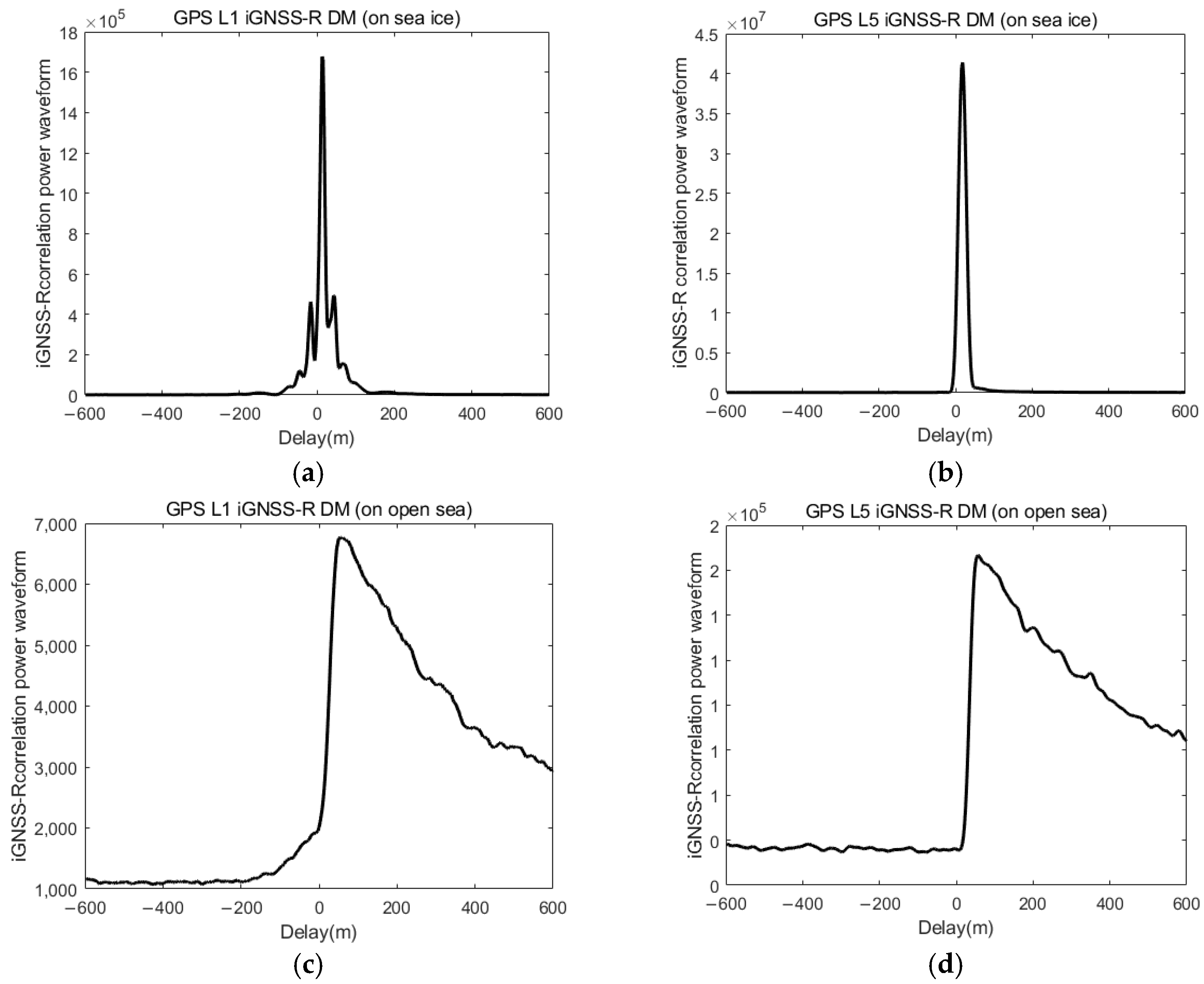
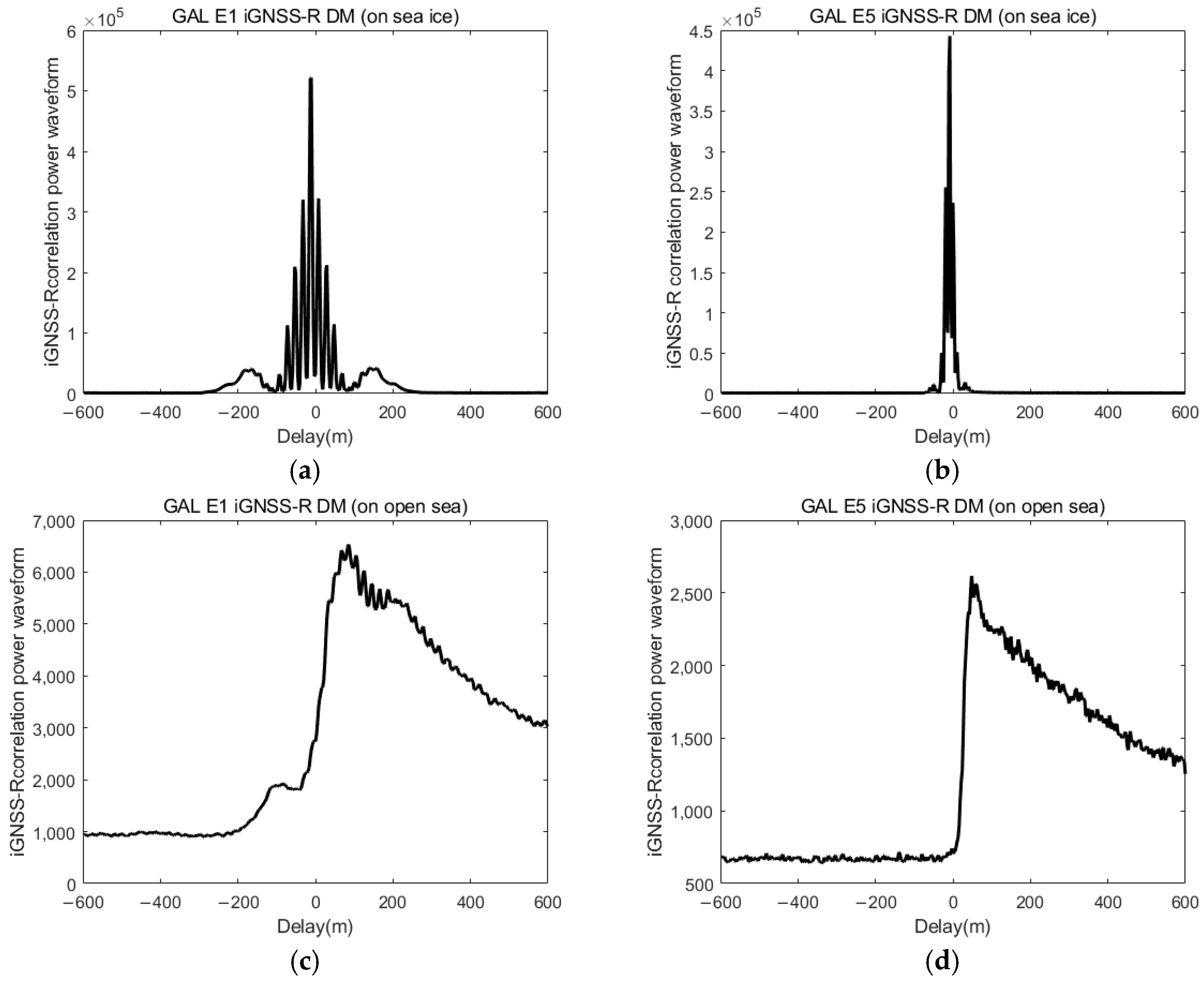
2.2. Interferometric Waveforms Description

The iGNSS-R interferometric waveform is the main measurement employed by the NSSC iGNSS-R altimeter for high-precision interferometric altimetry. They are 1D delay correlation power mappings (DMs) which correspond to the 0 Doppler cuts of the traditional 2D delay–Doppler correlation power mappings. The interferometric waveform is generated at a frequency of 5 Hz (i.e., one interferometric waveform every 0.2 s). Each interferometric waveform has a coherent integration time of 1 millisecond and undergoes 200 times of incoherent accumulation to reduce noise. The waveform consists of 448 time delay sampling points with a sampling rate of 112 MHz. The time delay between adjacent sampling points corresponds to a spatial distance of approximately 2.6767 m, covering a total range window of about ±600 m. The frequency bands are L1 and L5 for GPS, B1 and B2 for BDS, and E1 and E5 for the Galileo system. The main parameters used by the NSSC iGNSS-R altimeter to form the interferometric DMs can be found in

Table 1. Main parameters of NSSC iGNSS-R altimeter interferometric waveforms.

Parameters	Values
Frequency	GPS L1/L5, BDSB1/B2, GAL E1/E5
Beam	16 (4 direct L1/B1/E1, 4 direct L5/E5/B2, 4 reflected L1/B1/E1, 4 reflected L5/E5/B2)
DMs	5 Hz 448 delay tags Delay coverage: ±600 m Delay tag interval: 2.6767 m (112 MHz)
Coherent time	1 ms
Incoherent times	200
Band width	B1: 32 MHz, B2: 44 MHz L1: 26 MHz, L5: 20 MHz E1: 32 MHz, E5: 44 MHz

.

Since its launch in 2023, the NSSC iGNSS-R altimeter has collected a vast amount of interferometric waveforms from the BDS, GPS, and GAL systems. Figure 2, Figure 3 and Figure 4 present the typical coherent and incoherent interferometric waveforms collected on the sea ice surface and open ocean surface, corresponding to BDS, GPS, and GAL, respectively.

As is evident from Figure 2, Figure 3 and Figure 4, the utilization of GNSS broadband ranging codes in iGNSS-R yields two characteristic improvements in DMs: (1) steepened leading-edge slopes across all observed waveforms; and (2) multi-peak structures attributable to the incorporation of multiple code types. Particularly for sea ice observations, the DMs exhibit enhanced coherence in reflected signals. The spaceborne-acquired waveforms exhibit remarkable consistency with the land-based experimental waveforms reported in [44].

To more clearly illustrate the differences between GNSS-R interferometric waveforms and traditional GNSS-R DDM measurements, Figure 5 demonstrates the simultaneous acquisition of both DDM waveforms and dual-frequency interferometric waveforms from the same GPS PRN 3 satellite, obtained through the interferometric altimetry mode and the DDM measurement mode of the iGNSS-R altimeter, respectively. GPS L1 Coarse/Acquisition (C/A) code signals were employed for GNSS-R DDM measurements.The DDM has a size of 61 × 20, with a time delay interval of 1/8 chip, encompassing 61 sampling points. The Doppler frequency interval is 500 Hz, covering 20 sampling points. The specular point predicted by the model is designed to be at the center of the DDM waveform. The coherent integration time for the DDM waveforms is 1 millisecond, with each output waveform being the result of 1000 non-coherent accumulations, yielding an output rate of 1 Hz.

For comparative analysis, Figure 5d shows the DM waveform at 0 Hz Doppler frequency extracted from the DDM waveform in Figure 5c. Due to significant amplitude variations among the three DM waveforms, the y-axis in Figure 5 displays the Signal-to-Noise Ratio (SNR) for standardized comparison.

Comparative analysis in Figure 5 reveals that, for given sea conditions and antenna gain parameters, interferometric waveforms possess markedly steeper leading edges. This geometric characteristic is principally responsible for high-precision altimetry through interferometric approaches.

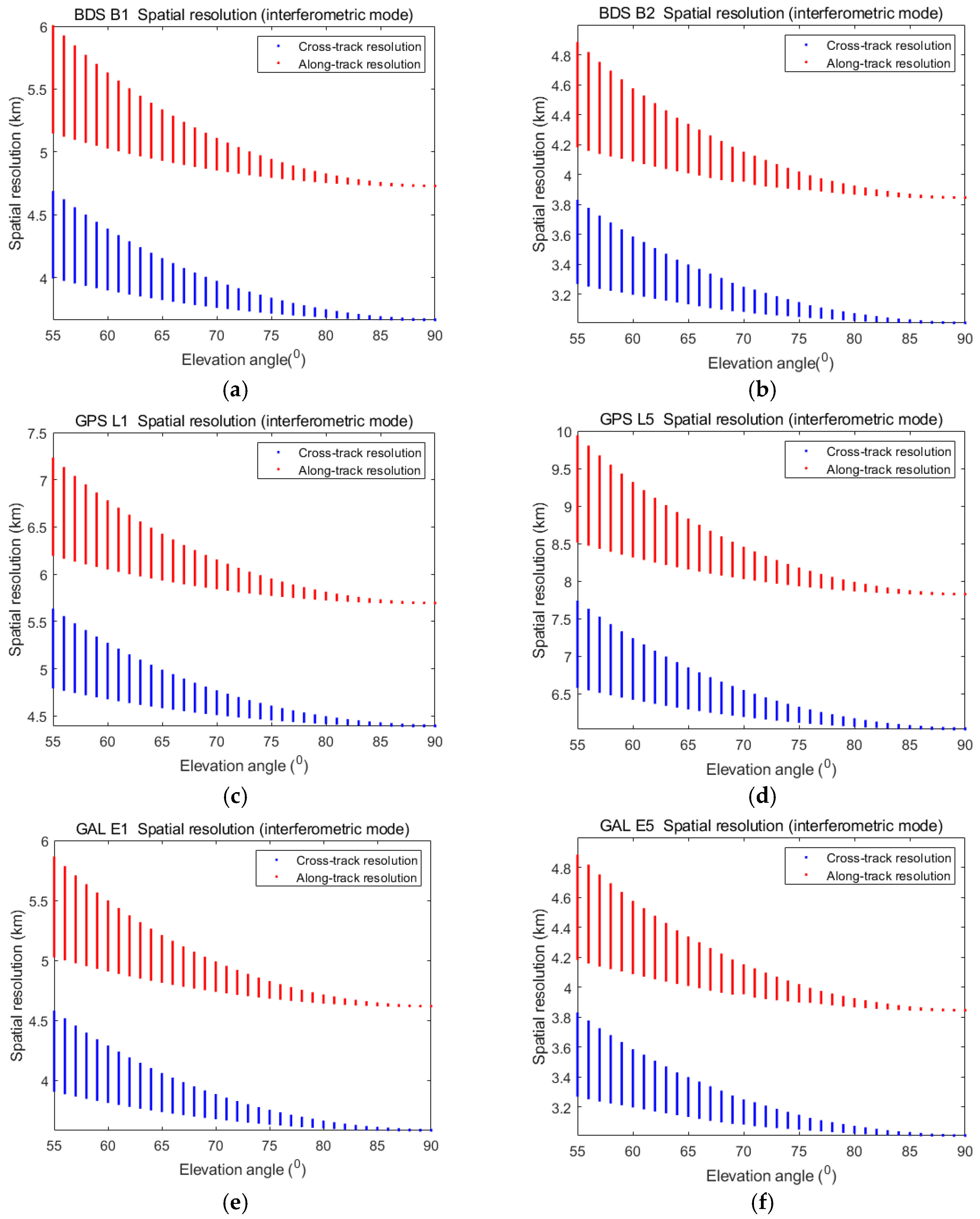
2.3. Spatial Resolution

The cross-track spatial resolution of the iGNSS-R altimeter in this experiment was primarily determined by the hybrid-code ambiguity function (using the half-power beamwidth criterion). Based on the satellite’s orbital altitude, we conducted simulations to evaluate the minimum resolution cells for the BDS, GPS, and Galileo systems across elevation angles ranging from 55° (incidence angle = 35°) to 90° (incidence angle = 0°) and azimuth angles ranging from 0° to 360°. The simulation results are shown in Figure 6. As can be seen from the figure, the minimum cross-track resolution and along-track spatial resolution of BDS and GAL are relatively close, with the cross-track resolution being less than 4.75 km and the along-track resolution being better than 6 km. In contrast, the cross-track resolution of GPS is less than 7.75 km, and the along-track resolution is less than 10 km.

To mitigate the effects of speckle noise and enhance altimetry accuracy, it is essential to apply incoherent accumulation processing to the DM waveform and to smooth the sea surface height in the along-track direction. Consequently, the along-track spatial resolution of the iGNSS-R altimetry product is contingent upon the duration of along-track incoherent accumulation and the extent of sea surface height smoothing. The iGNSS-R altimeter has a sampling rate of 5 Hz, meaning that incoherent processing has already been performed for 0.2 s onboard. Since the average moving speed of the specular point is about 5.6 km/s, the cross-track and along-track spatial resolutions shown in Figure 6 correspond to the cross-track and along-track spatial resolutions of a single DM waveform. The purpose of this experiment was to verify the interferometric altimetry accuracy under a spatial resolution of 40 km. Therefore, after inverting the sea surface height using the 5 Hz DM waveform, it was necessary to smooth the sea surface height over an along-track distance of 40 km. In summary, the along-track resolution of the final iGNSS-R sea surface height was close to 40 km.

2.4. iGNSS-R Sea Surface Height Retrieval

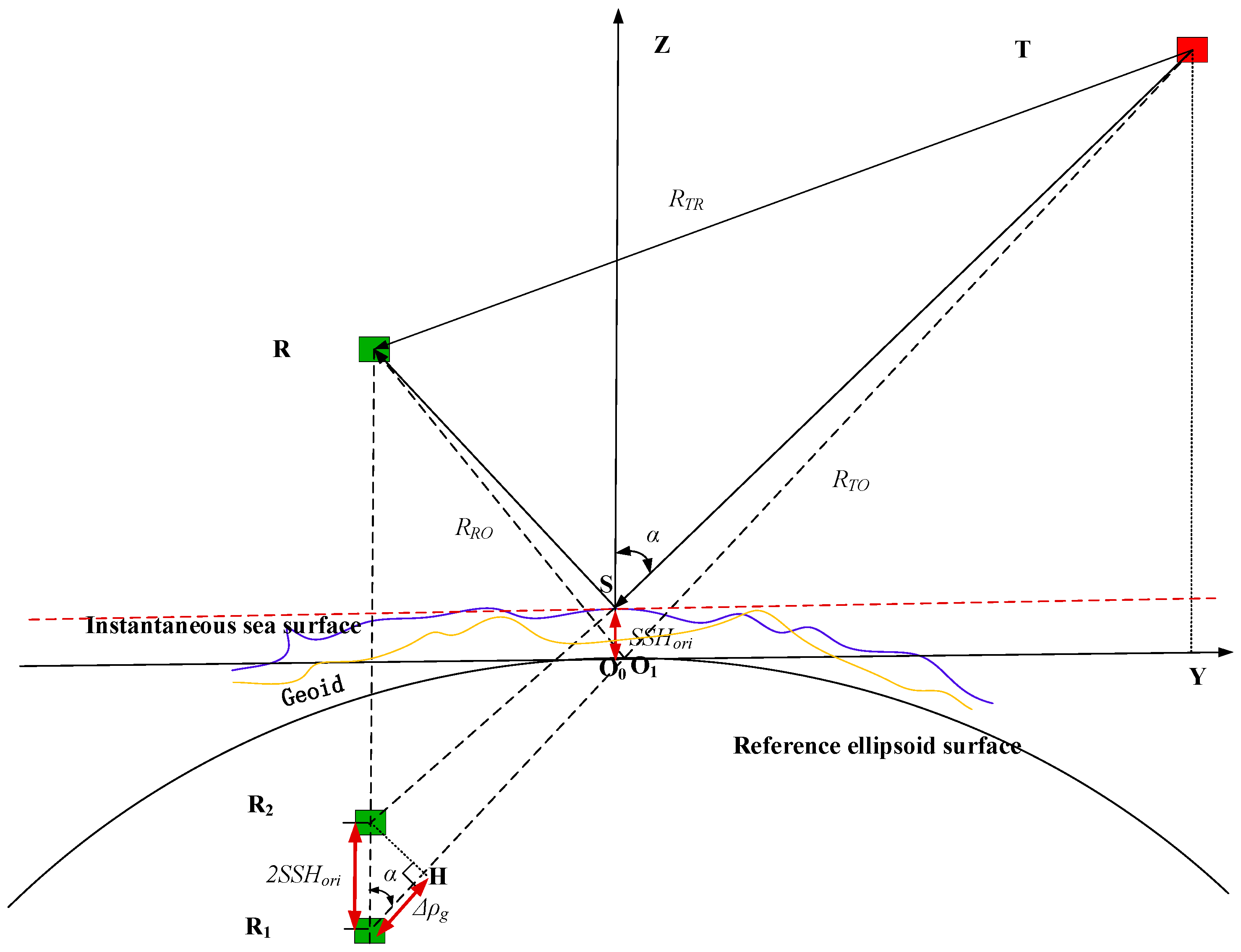
2.4.1. Geometry Model for iGNSS-R SSH Calculation

The geometry model for iGNSS-R SSH calculation is illustrated in Figure 7.

In Figure 7, T denotes a GNSS satellite, R represents a GNSS-R receiver, S indicates the sea surface specular point where the signal emitted by GNSS satellite T is reflected by the sea surface and received by iGNSS-R altimeter R, O₁ is the theoretical sea surface specular point on the reference ellipsoid surface, O₀ is the projection point of specular point S onto the reference ellipsoid surface, and α represents the incidence angle. The distance between O₀ and S is the height of the GNSS-R specular point relative to the reference ellipsoid surface, which is the instantaneous SSH (SSH_ori) measurable by GNSS-R. Points R₁ and R₂ represent the mirror images of receiver R relative to the ellipsoid surface and sea level, respectively. According to the mirror image principle, the distance between R₁ and R₂ equals twice the SSH_ori.

The formula for calculating the GNSS-R SSH_ori is as follows [44]:

$${SSH}_{ori}={\displaystyle \frac{∆{\rho }_g}{2cos\alpha }}={\displaystyle \frac{\left({\rho }_{geo}^{ro}-{\rho }_{geo}^{do}\right)-c∆\tau }{2cos\alpha }}+{\displaystyle \frac{{\rho }_{trop}^r+\left({\rho }_{ion}^r-{\rho }_{ion}^d\right)+{\rho }_{rough}^r+{\rho }_{instru}^{rd}+{\epsilon }^{rd}}{2cos\alpha }}$$

(1)

where $∆{\rho }_g$ is the geometric distance difference of TR₁ and TR₂ in the geometry model; ${\rho }_{geo}^{ro}$ represents the sum of the distance from the GNSS satellite to O1 and the geometric distance from O1 to the iGNSS-R altimeter R; ${\rho }_{geo}^{do}$ is the geometric distance between the iGNSS-R altimeter R and the GNSS satellite T; c is the speed of light; Δτ is the measured propagation delay difference between the GNSS sea surface reflected signal and the direct signal, and is measured utilizing the leading edge of the iGNSS-R DM in this study; ${\mathsf{\rho }}_{\mathrm{t}\mathrm{r}\mathrm{o}\mathrm{p}}^{\mathrm{r}}$ accounts for the tropospheric delay of the GNSS reflection path, including dry and wet tropospheric delays; ${\rho }_{ion}^r$ and ${\rho }_{ion}^d$ represent the ionospheric delays along GNSS reflection path and direct path, respectively; ${\rho }_{rough}^r$ accounts for the electromagnetic deviation caused by sea surface roughness; ${\rho }_{instru}^{rd}$ is the receiver hardware delay; and ${\epsilon }^{rd}$ is the ranging error caused by the measurement error of Δτ.

Similarly to the radar altimeter, after obtaining the instantaneous sea surface height SSH_ori, it is necessary to apply geophysical corrections to it to compare measurements at different times or compare measurements to the mean sea surface, removing the influence of factors such as ocean tides, polar tides, solid Earth tides, and dynamic atmospheric correction (DAC) in order to obtain the final SSH.

2.4.2. DM Waveform Matching

We employed the waveform matching method to determine the time delay of the specular point in the iGNSS-R DM waveform. The theoretical waveform library used in this process was generated through simulation using the GREEPS software [46]. Figure 8 presents a set of results from the matched BDS iGNSS-R DM waveforms. Given that waveform matching is a computationally intensive process, we implemented multithreading technology to significantly enhance the matching efficiency.

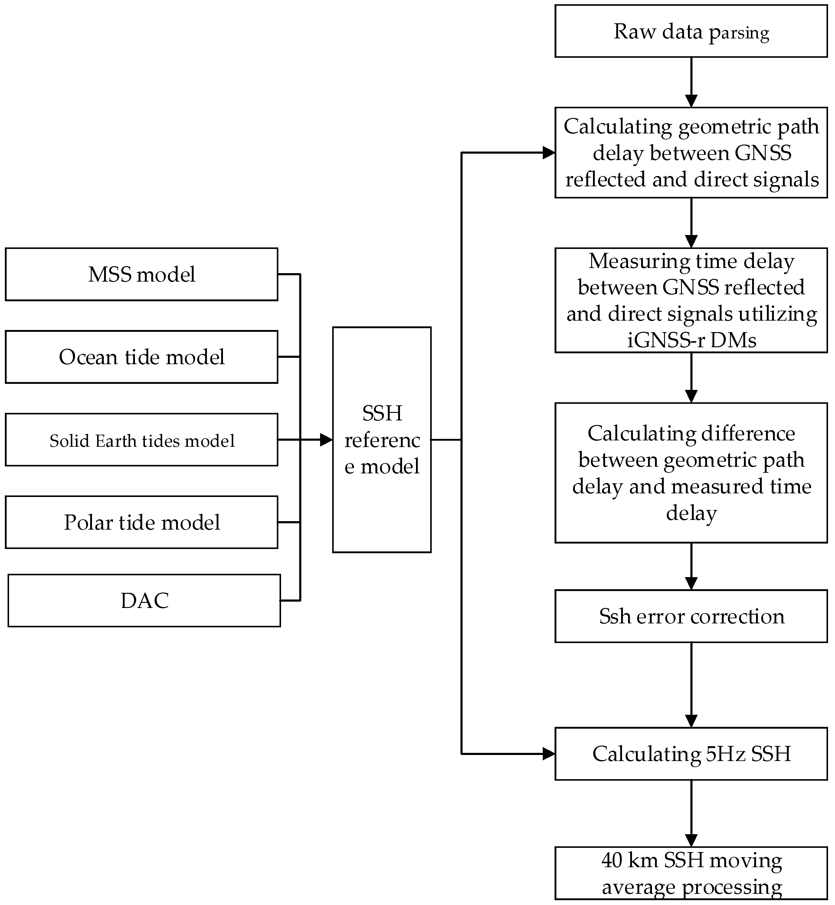
2.4.3. The Process of iGNSS-R SSH Retrieval

The flowchart of the iGNSS-R SSH inversion is depicted in Figure 9, and encompasses the following steps:

(1)

Data Parsing: Dual-frequency iGNSS-R DMs and auxiliary information are extracted from raw data packets.

(2)

Geophysical Path Delay Calculation: Utilizing the preliminary geolocation of the specular point calculated onboard, the SSH reference model is computed, incorporating the mean sea surface height, ocean tide, solid Earth tide, polar tide, and DAC. The specular point position is recalculated using the SSH reference model, precise GNSS ephemeris, and precise orbit determination files. Phase center corrections are applied to direct and reflected GNSS signals using satellite attitude information, and the geometry model delay difference between the GNSS reflected and direct signals is calculated.

(3)

Measuring Time Delay: The waveform-matching method is employed to determine the measured delay difference between GNSS reflected and direct signals. Corrections are applied, using a hardware delay lookup table, to the measured time delay difference between the reflected and direct GNSS signals.

(4)

Calculating the Delay Difference: The difference between the geophysical path delay and the measured time delay is calculated.

(5)

SSH_ori Error Correction and Calibration: The instantaneous sea surface height (SSHori) is calculated using (1). To eliminate the impact of ionospheric bias, a dual-frequency combination technique is employed. The dry and wet tropospheric delays are computed using the European Centre for Medium-Range Weather Forecasts (ECMWF) reanalysis data (temperature, humidity, and air pressure) through ray-tracing techniques that account for atmospheric variations along the reflection path. In [47,48], Ghavidel et al. utilized numerical simulations to calculate the electromagnetic (EM) bias of L-band waves using the physical optics (PO) method under the Kirchhoff approximation (KA). They examined the impacts of several factors, including the incidence angle, wind speed, rain, swell, and surface currents. Their findings indicate that significant wave height, sea surface wind speed, and the incidence angle are the main contributors to EM bias, with the effect of the incidence angle being well-described by a cosine function. Based on these results, we developed an EM bias lookup table to correct for sea state bias. After correcting for the aforementioned errors, the residual error compared with radar altimeter data are modeled according to the cosine function of the incidence angle to calibrate the SSHori.

(6)

Calculation of 5 Hz SSH: After SSH_ori error correction and calibration, the GOT4.10 model is used to correct for ocean tides. Polar tides, which are tidal phenomena caused by the centrifugal effect due to the motion of the Earth’s poles, are corrected using the International Earth Rotation and Reference Systems Service (IERS) polar tide model. Solid Earth tides are corrected using the tidal response analysis proposed in [49]. DAC is applied using the DAC data released by AVISO (https://www.aviso.altimetry.fr/en/data.html (accessed on 20 May 2025)).

(7)

40 km SSH Moving Average Processing: Utilizing the 5 Hz SSH data, 40 km along-track averaging is implemented to achieve the final SSH products. The main steps of the along-track averaging are as follows: First, the difference between the 5 Hz sea surface height measurements and the corresponding mean sea surface height model is calculated. Next, this difference is smoothed to a 40 km resolution. Finally, the smoothed difference is added back to the mean sea surface height model value to obtain the 40 km sea surface height product.

2.5. Inter-Satellite Cross-Validation Method

2.5.1. iGNSS-R Altimeter Products

The iGNSS-R altimeter experiment data used for inter-satellite cross-validation in this study were collected from 11 July 2023 to 29 December 2023. The data feature a sampling rate of 5 Hz and an along-track spatial resolution of 40 km. For inter-satellite cross-validation with radar altimeter products, sea surface heights and several error correction parameters were extracted from these data. These parameters include ocean tides, polar tides, solid Earth tides, DAC, and dry and wet tropospheric correction terms.

2.5.2. Jason-3 Satellite Radar Altimeter Products

Launched on 17 January 2016, the Jason-3 satellite is an international cooperative altimetry mission jointly developed by the National Aeronautics and Space Administration (NASA), the National Oceanic and Atmospheric Administration (NOAA), the European Organization for the Exploitation of Meteorological Satellites (EUMETSAT), and the Centre National d’Études Spatiales (CNES). As a successor to the TOPEX/Poseidon and Jason-1 missions, Jason-3 continues a nearly 30-year legacy of high-accuracy sea level measurements. It is a non-Sun-synchronous satellite with a mean altitude of 1336 km, an inclination of 66°, and a repeat cycle of 9.9156 days.

Since the Jason-3 Geophysical Data Records (GDRs) have undergone rigorous calibration and validation using in situ measurements and cross-satellite comparisons, we utilized Jason-3 Level 2 GDR 1 Hz data (from 1 July to 31 December 2023) to evaluate the accuracy of the NSSC iGNSS-R altimeter data products.

2.5.3. Sensial-6 Satellite Radar Altimeter Products

Sentinel-6, launched on 21 November 2020, operates at a mean altitude of 1336 km with an inclination of 66°. Its primary payload, the Poseidon-4 SAR altimeter, operates in the Ku- and C-band, with the latter primarily used for ionospheric corrections.

Poseidon-4 provides three types of Level 2 sea surface height (SSH) products: Near-Real-Time (NRT), Short-Time-Critical (STC), and Non-Time-Critical (NTC). These products are disseminated within 2 h, 36 h, and 60 days after data acquisition, respectively. In this study, the Level 2 NTC 1 Hz SSH product (from 1 July to 31 December 2023) was used to evaluate the accuracy of the NSSC iGNSS-R altimeter SSH products.

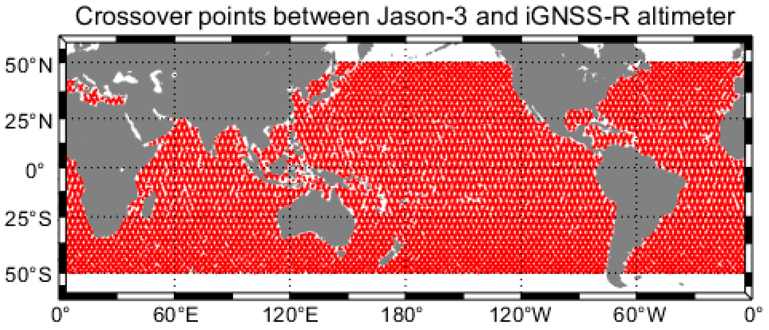
2.5.4. Crossover Data Calculation Method

In this study, we selected the near-observation point interpolation method for crossover data calculation [50]. This approach effectively mitigates inaccurate or erroneous assessments that may arise from imprecise positioning measurements at crossover points. To match the 40 km spatial resolution of the iGNSS-R altimeter SSH products, we applied an approximately 40 km smoothing filter to consecutive 1 Hz altimeter measurements prior to interpolation.

Rigorous data preprocessing was conducted, including temporal and spatial matching with radar altimeter data within a 3-day time window for SSH, a 0.2 h time window for ocean tides, pole tides, solid Earth tides, and DACs, and a 0.5 h time window for dry/wet tropospheric delay corrections.

In this study, we evaluated the bias, standard deviation (STD), root mean square error (RMSE), and correlation coefficient (R) of sea surface height, as well as several error correction parameters, including ocean tide, polar tide, solid Earth tide, DAC, and dry and wet tropospheric correction terms. It should be noted that the assessment results for the dry and wet tropospheric correction terms are only applicable to the case where the incidence angle is 0°. For other incidence angles, the assessment results at a 0° incidence angle should be divided by the cosine of the incidence angle to obtain equivalent evaluations.

The statistical parameters were calculated using the following equations:

$$Bias={\displaystyle \frac{1}{N}}\sum _{i=1}^N\left(R_i-A_i\right)$$

(2)

$$STD=\sqrt{{\displaystyle \frac{{\sum }_{i=1}^N{\left(R_i-A_i-\overline{R-A}\right)}^2}{N-1}}}$$

(3)

$$RMSE=\sqrt{{\displaystyle \frac{{\sum }_{i=1}^N{\left(R_i-A_i\right)}^2}{N}}}$$

(4)

$$R={\displaystyle \frac{{\sum }_{i=1}^N\left(R_i-\overline{R}\right)\left(A_i-\overline{A}\right)}{\sqrt{{\sum }_{i=1}^N{\left(R_i-\overline{R}\right)}^2{\sum }_{i=1}^N{\left(A_i-\overline{A}\right)}^2}}}$$

(5)

where N is the number of collocations, $R_{\mathrm{i}}$ is the GNSS-R SSH measurements, and $A_{\mathrm{i}}$ is the radar altimeter measurement. Together, these four statistical parameters are capable of characterizing the error property of the iGNSS-R measurements.

3. Results

This section characterizes the iGNSS-R altimeter SSH and quantifies its measurement accuracy by comparison with Jason-3 and Sentinel-6 reference data. The evaluation additionally encompasses the accuracy assessment of critical error correction components: ocean tide, polar tide, solid Earth tide, DAC, and dry/wet tropospheric corrections.

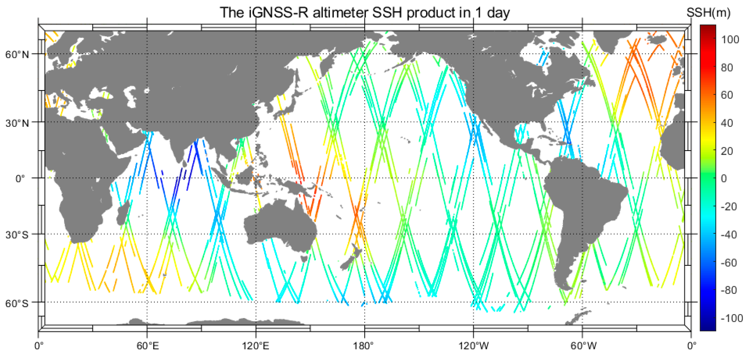
3.1. Routine Daily SSH Products from iGNSS-R Altimeter

Unlike conventional radar altimeters that provide continuous along-track measurements, GNSS-R interferometric altimetry produces segmented observations with variable durations dependent on the elevation angles of visible GNSS satellites. Tracking of individual satellites terminates when their incidence angles fall below 35°, at which point the system switches to alternate satellites. Figure 10 demonstrates the typical daily distribution pattern of these GNSS-R interferometric altimetry products. The system’s capability to simultaneously track up to four GNSS satellites enables concurrent observation of up to four distinct sea surface height swaths, representing a key advantage over traditional single-beam altimeters.

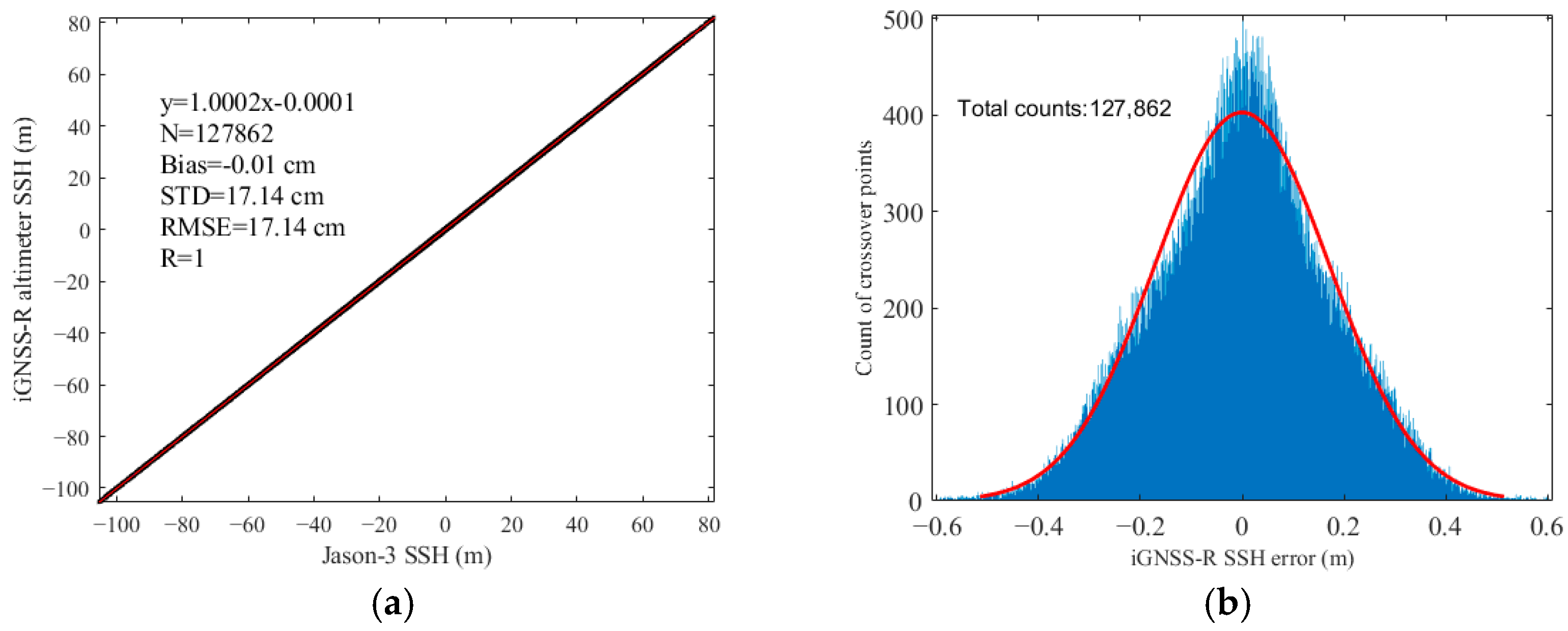
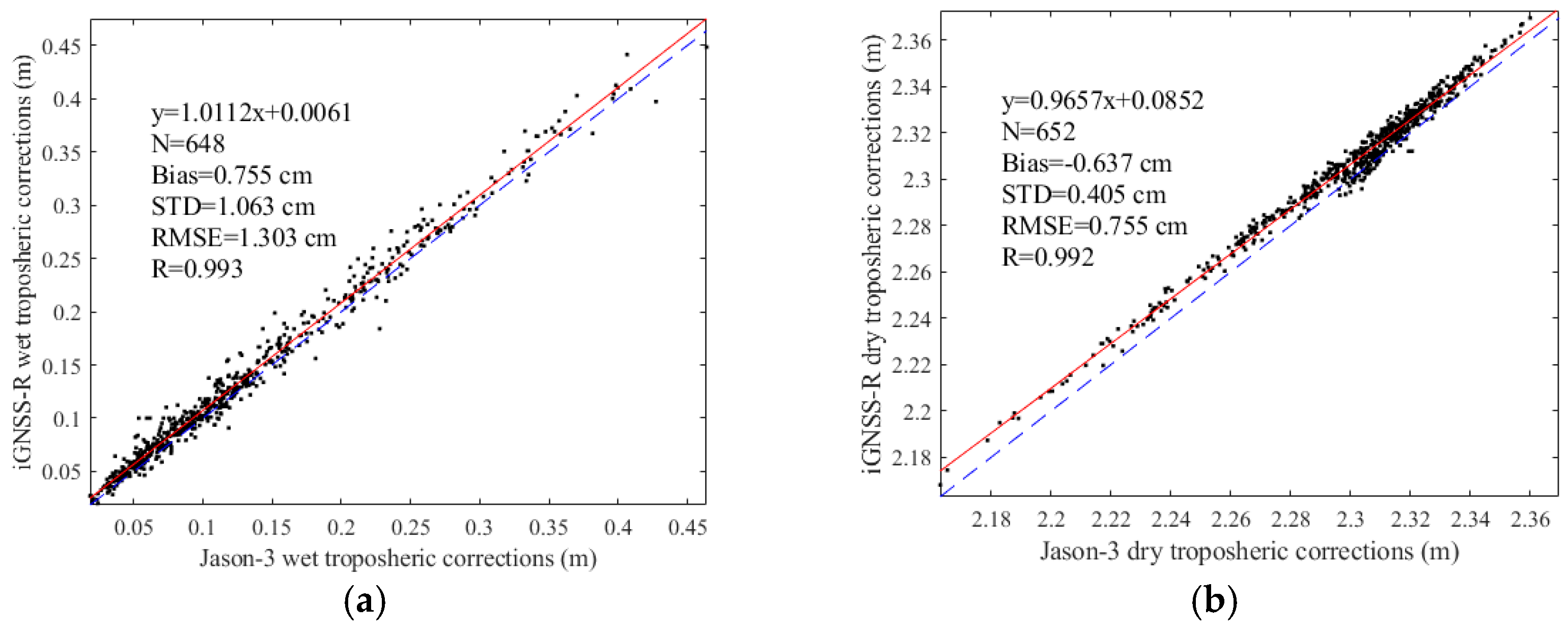
3.2. Intercomparisons with Jason-3 SSH Products

During the study period from 11 July to 29 December 2023, we identified 127,862 crossover points for SSH product accuracy assessment. Figure 11 presents their global distribution, limited to ±50° latitude to exclude potential sea ice effects (the iGNSS-R altimeter’s full observational range extends to ±81° latitude). The distribution demonstrates comprehensive coverage across all major ocean basins within this latitudinal zone.

Figure 12 presents the evaluation of iGNSS-R SSH against Jason-3 SSH at crossover points. Figure 12a shows the scatter plot comparison between the two datasets. To better illustrate the retrieval errors of iGNSS-R SSH, Figure 12b displays the statistical distribution of errors across 127,862 crossover points. The results indicate that the iGNSS-R SSH has a root mean square error (RMSE) of 17.14 cm and a bias of −0.01 cm, with the overall error distribution closely approximating a normal distribution (Gaussian).

Figure 13 presents the evaluation results of iGNSS-R altimeter SSH error corrections using Jason-3-derived parameters at crossover points, including dry/wet tropospheric delays, ocean tides, pole tides, solid Earth tides, and DAC. In the subfigures, the blue dashed lines represent the 1:1 lines, while the red solid lines show the results of the least-squares linear fit. With a 0.2 h time window for ocean tides, pole tides, solid Earth tides, and DAC matching, 668 crossover points were available for comparison. With a 0.5 h time window for dry/wet tropospheric delay correction matching, 650 crossover points were available for comparison.

Figure 13a,b show RMSEs of 1.303 cm for wet tropospheric delay correction and 0.755 cm for dry tropospheric delay correction at a 0° incidence angle. When scaled by the cosine of the incidence angle to account for the maximum 35° viewing geometry of iGNSS-R, these errors increase to 1.59 cm (wet) and 0.92 cm (dry), respectively.

Figure 13c–f reveal RMSEs for other correction terms: 3.23 cm (ocean tide), 0.49 cm (pole tide), 0.43 cm (solid Earth tide), and 0.39 cm (DAC).

Table 2. Comparative assessment with Jason-3 SSH products.

Validation Parameters	STD (cm)	Bias (cm)	RMSE (cm)	R
SSH	17.140	−0.010	17.140	1
Wet tropospheric delay *	1.063	0.755	1.303	0.993
Dry tropospheric delay *	0.405	−0.637	0.755	0.992
Ocean tide	3.225	−0.219	3.230	0.994
Polar tide	0.492	−0.003	0.492	0.902
Solid earth tide	0.435	−0.002	0.434	0.998
DAC	0.390	−0.013	0.390	1

* Statistical results at 0° incidence angle.

summarizes the overall accuracy assessment of iGNSS-R SSH products, using Jason-3 as reference.

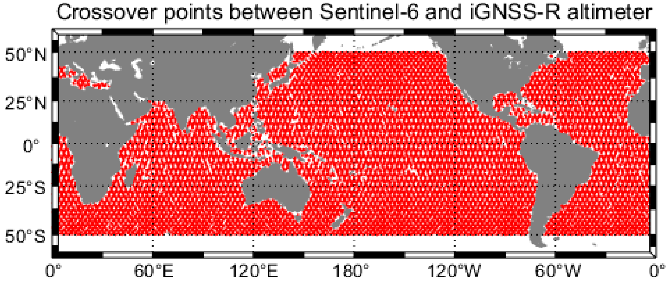
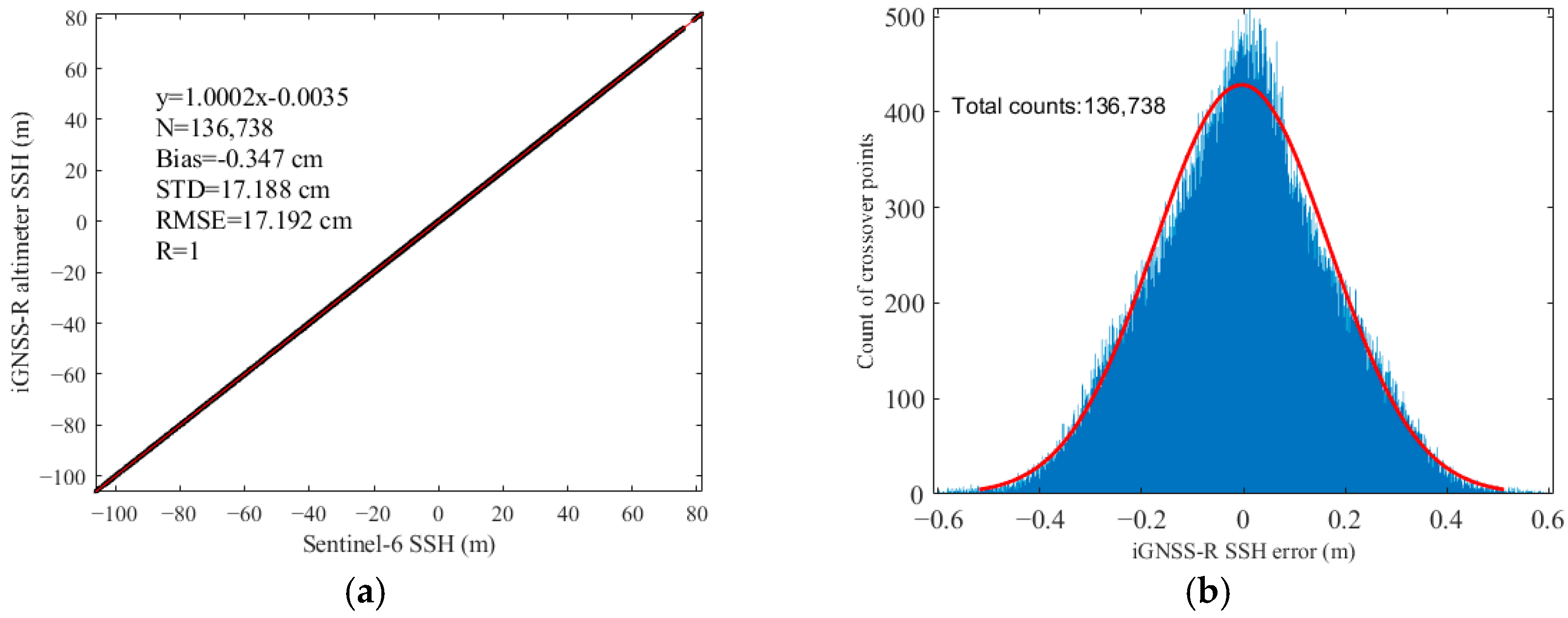
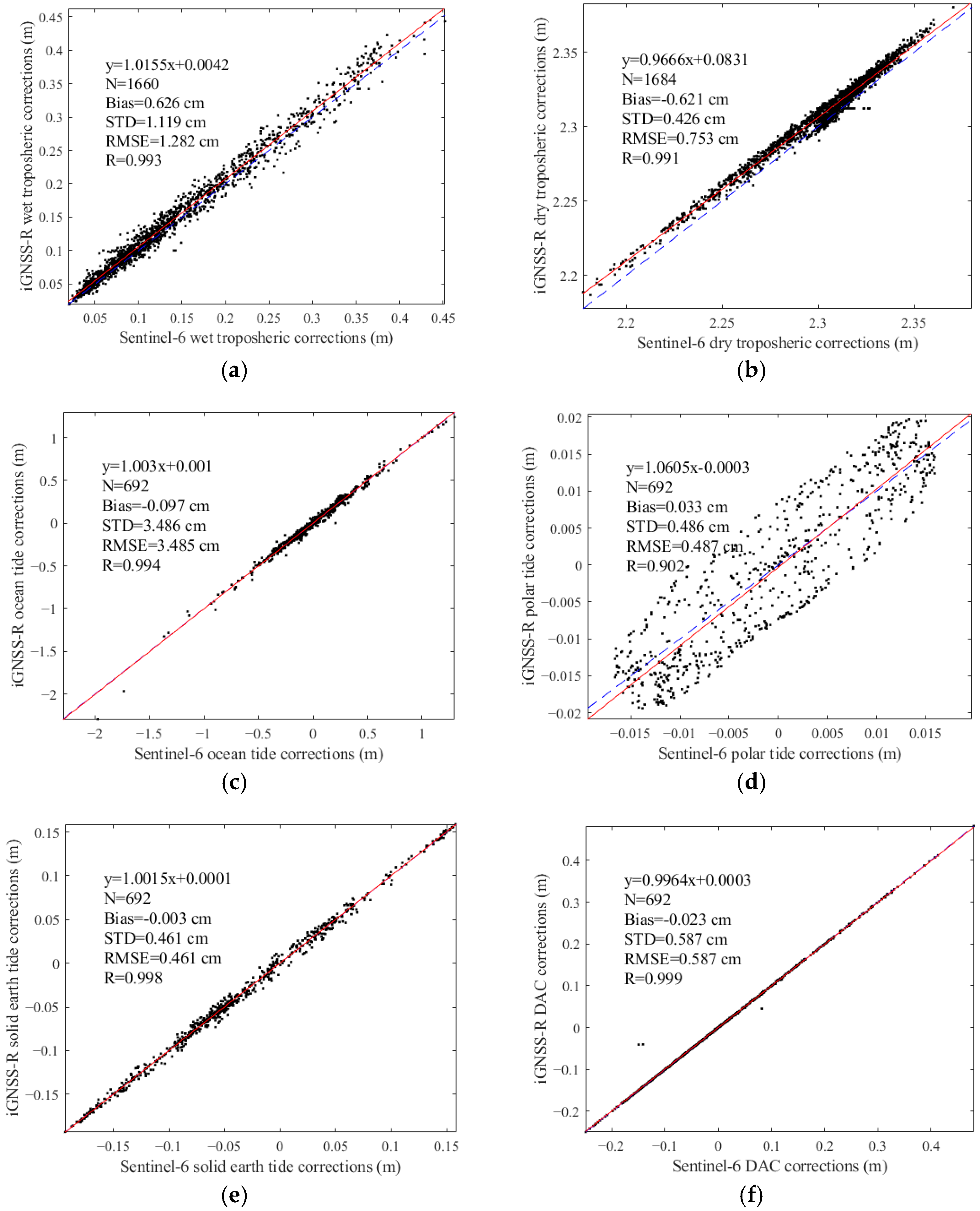
3.3. Intercomparisons with Sentinel-6 SSH Products

During the study period (11 July–29 December 2023), we identified 136,738 crossover points for SSH product accuracy assessment. Figure 14 shows their global distribution, demonstrating similar spatial patterns between Sentinel-6/iGNSS-R altimeter and Jason-3/iGNSS-R altimeter pairs. This similarity stems from nearly identical orbital parameters, with Sentinel-6’s orbit offset by ~157 km (half the intertrack distance) from Jason-3. This deliberate offset improves spatial sampling and enhances both the coverage and representativeness of our SSH evaluation.

Figure 15 presents the evaluation of iGNSS-R SSH against Sentinel-6 SSH at crossover points. Figure 15a shows the scatter plot comparison between the two datasets. To better illustrate the retrieval errors of iGNSS-R SSH, Figure 15b displays the statistical distribution of errors across 136738 crossover points. The results indicate that the iGNSS-R SSH has an RMSE of 17.19 cm and a bias of −0.35 cm, with the overall error distribution closely approximating a normal distribution. Compared to the evaluation based on Jason-3 data, the SSH deviations derived from Sentinel-6 data exhibit slightly larger magnitudes. This difference primarily originates from our calibration methodology, in which Jason-3 data were used as the reference standard for SSH calibration.

Figure 16 presents the evaluation results of iGNSS-R altimeter SSH error corrections using Sentinel-6-derived parameters at crossover points, including dry/wet tropospheric delays, ocean tide, pole tide, solid Earth tide, and DAC. In the subfigures, the blue dashed lines represent the 1:1 lines, while the red solid lines show the results of the least-squares linear fit. With a 0.2 h time window for ocean tide, pole tide, solid Earth tide, and DAC matching, 692 crossover points were available for comparison. With a 0.5 h time window for dry/wet tropospheric delay correction matching, more than 1660 crossover points were available for comparison. Due to orbital geometry, the number of crossover points available for dry/wet tropospheric delay evaluation was approximately 2.5 times greater for Sentinel-6 than for Jason-3.

Figure 16a,b show RMSEs of 1.282 cm for wet tropospheric delay correction and 0.753 cm for dry tropospheric delay correction at a 0° incidence angle. When scaled by the cosine of the incidence angle to account for the maximum 35° viewing geometry of iGNSS-R, these errors increase to 1.57 cm (wet) and 0.92 cm (dry), respectively.

Figure 16c–f reveal the RMSEs for the other correction terms: 3.49 cm (ocean tide), 0.49 cm (pole tide), 0.46 cm (solid Earth tide), and 0.59 cm (DAC).

Table 3. Intercomparison results with Sentinel-6 SSH products.

Validation Parameters	STD (cm)	Bias (cm)	RMSE (cm)	R
SSH	17.188	−0.347	17.192	1
Wet tropospheric delay *	1.119	0.626	1.282	0.993
Dry tropospheric delay *	0.426	−0.621	0.753	0.991
Ocean tide	3.486	−0.097	3.485	0.994
Polar tide	0.486	0.033	0.487	0.902
Solid Earth tide	0.461	−0.003	0.461	0.998
DAC	0.587	−0.023	0.587	0.999

* Statistical results at 0° incidence angle.

summarizes the overall accuracy assessment of the iGNSS-R SSH products, using Sentinel-6 as a reference.

4. Discussion

Unlike traditional altimeters, iGNSS-R offers wide-swath coverage, exceeding even SWOT’s swath width. However, its observations contain gaps due to limited beam counts. This study’s validation payload tracked up to four beams simultaneously, but geometric analysis suggests that 14–15 satellites could be tracked at 35° incidence by expanding the beam capacity. Combined with iGNSS-R’s low-cost advantage, multi-satellite constellations could further enhance spatial coverage. Based on the simulation results in Section 2.3, the iGNSS-R system achieves an average spatial resolution of 9 km for GPS and 5 km for BDS/Galileo within 35° incidence angles, comparable to Jason-3 and Sentinel-6’s low-resolution mode (LRM), though inferior to Sentinel-6’s SAR mode and SWOT. Nevertheless, this successful in-orbit validation demonstrates iGNSS-R’s potential for high-resolution (5–10 km) ocean remote sensing products (e.g., sea surface height, wind speed, and significant wave height).

Preliminary assessments using Jason-3 and Sentinel-6 data showed that the iGNSS-R altimeter achieves an SSH accuracy of 17.2 cm@40 km, which is a breakthrough for GNSS-R altimetry. Notably, current operational GNSS-R missions (e.g., CYGNSS, Spire) remain constrained to meter-level altimetry accuracy, due to their inherent reliance on narrow-bandwidth local code correlation processing schemes [10,17,18,19,20,21]. However, when equivalently scaled to 5 km along-track smoothing, the altimetric error of the iGNSS-R altimeter is about 48.65 cm, which is over an order of magnitude higher than that of conventional radar altimeters. In the future, further improvements in accuracy and synergistic use with existing altimeters require deeper study.

Compared with the SSH RMSE, error contributions from tides, DAC, and tropospheric delays are minor. The impacts of ionospheric delay and sea state bias require further validation, due to the current lack of reliable in situ reference data. While quantitative assessments of sea state bias and ionospheric errors are not addressed here, instrument noise and speckle errors—which directly degrade interferometric waveform quality—are the dominant error sources [51,52,53,54,55]. These errors exhibit strong dependencies on the GNSS constellation, signal frequency, bandwidth, incident angle, SNR, PRN code, and so on [56,57,58]. Given the complexity of these relationships, a detailed analysis will be presented in a subsequent study.

5. Conclusions

The first spaceborne demonstration of iGNSS-R altimetry via the 2023 Chinese satellite mission has validated its operational feasibility for global ocean monitoring. Our crossover validation with Jason-3 and Sentinel-6 reveals an unprecedented altimetric accuracy of 17.2 cm at 40 km resolution, representing a breakthrough improvement over previous GNSS-R missions and establishing a new benchmark for GNSS-R altimetry.

Compared to traditional altimeters and SWOT’s single-pass performance, iGNSS-R technology shows clear disadvantages in measurement precision. However, the successful demonstration of the iGNSS-R technology opens up new possibilities for cost-effective, wide-swath sea level monitoring; its unique advantages—including an observation swath exceeding 1000 km and rapid global coverage/revisit capability—present opportunities for complementary use with existing altimetry systems and enhance our understanding of global sea surface dynamics.

Future work will focus on further refining the SSH retrieval model and error correction methods presented in this study in order to achieve optimal performance, and on validating the impacts of ionospheric delay and sea state bias. Notably, iGNSS-R has also demonstrated strong coherent characteristics over polar ice surfaces, where its altimetric accuracy and spatial resolution are expected to surpass those over ocean surfaces. Exploring iGNSS-R’s applications in polar ice detection will be an important focus of future research.

References

1. Srinivasan, M.; Tsontos, V. Satellite Altimetry for Ocean and Coastal Applications: A Review. Remote Sens. 2023, 15, 3939. [Google Scholar] [CrossRef]
2. Yang, L.; Lin, L.N.; Fan, L.; Liu, N.; Huang, L.Y.; Xu, Y.S.; Mertikas, S.P.; Jia, Y.J.; Lin, M.S. Satellite Altimetry: Achievements and Future Trends by a Scientometrics Analysis. Remote Sens. 2022, 14, 3332. [Google Scholar] [CrossRef]
3. Yao, J.Q.; Xu, N.; Wang, M.R.; Liu, T.; Lu, H.; Cao, Y.Q.; Tang, X.M.; Mo, F.; Chang, H.Y.; Gong, H.Y.; et al. SWOT satellite for global hydrological applications: Accuracy assessment and insights into surface water dynamics. Int. J. Digit. Earth 2025, 18, 2472924. [Google Scholar] [CrossRef]
4. Martín-Neira, M.; D’Addio, S.; Buck, C.; Floury, N.; Prieto-Cerdeira, R. The PARIS Ocean Altimeter In-Orbit Demonstrator. IEEE Trans. Geosci. Remote Sens. 2011, 49, 2209–2237. [Google Scholar] [CrossRef]
5. Huang, F.X.; Xia, J.M.; Yin, C.; Zhai, X.C.; Yang, G.L.; Bai, W.H.; Sun, Y.Q.; Du, Q.F.; Wang, X.Y.; Qiu, T.S.; et al. Spaceborne GNSS Reflectometry With Galileo Signals on FY-3E/GNOS-II: Measurements, Calibration, and Wind Speed Retrieval. IEEE Trans. Geosci. Remote Sens. Lett. 2023, 20, 3501505. [Google Scholar] [CrossRef]
6. Ruf, C.; Al-Khaldi, M.; Asharaf, S.; Balasubramaniam, R.; Mckague, D.; Pascual, D.; Russel, A.; Twigg, D.; Warnock, A. Characterization of CYGNSS Ocean Surface Wind Speed Products. Remote Sens. 2024, 16, 4341. [Google Scholar] [CrossRef]
7. Wang, F.; Yang, D.K.; Yang, L. Retrieval and Assessment of Significant Wave Height from CYGNSS Mission Using Neural Network. Remote Sens. 2022, 14, 3666. [Google Scholar] [CrossRef]
8. Yu, H.; Du, Q.F.; Xia, J.M.; Huang, F.X.; Yin, C.; Meng, X.F.; Bai, W.H.; Sun, Y.Q.; Wang, X.Y.; Duan, L.C.; et al. Comparative Analysis of SWH Retrieval Between BDS-R and GPS-R Utilizing FY-3E/GNOS-II Data. IEEE J. Sel. Top. Appl. Earth Obs. Remote Sens. 2025, 18, 6520–6531. [Google Scholar] [CrossRef]
9. Li, W.Q.; Cardellach, E.; Fabra, F.; Ribo, S.; Rius, A. Assessment of Spaceborne GNSS-R Ocean Altimetry Performance Using CYGNSS Mission Raw Data. IEEE Trans. Geosci. Remote Sens. 2020, 58, 238–250. [Google Scholar] [CrossRef]
10. Zhang, Y.; Huang, S.; Han, Y.L.; Yang, S.H.; Hong, Z.H.; Ma, D.H.; Meng, W.T. Machine Learning Methods for Spaceborne GNSS-R Sea Surface Height Measurement From TDS-1. IEEE J. Sel. Top. Appl. Earth Obs. Remote Sens. 2022, 15, 1079–1088. [Google Scholar] [CrossRef]
11. Hu, Y.; Hua, X.F.; Yan, Q.Y.; Liu, W.; Jiang, Z.H.; Wickert, J. Sea Ice Detection from GNSS-R Data Based on Local Linear Embedding. Remote Sens. 2024, 16, 2621. [Google Scholar] [CrossRef]
12. Yin, C.; Xia, J.M.; Huang, F.X.; Li, W.; Bai, W.H.; Sun, Y.Q.; Liu, C.L.; Yang, G.L.; Hu, X.Q.; Xiao, X.J.; et al. Sea Ice Detection with Fy3e Gnos Ii Gnss Reflectometry. In Proceedings of the 2021 IEEE Specialist Meeting on Reflectometry Using GNSS and Other Signals of Opportunity 2021 (Gnss+R 2021), Virtual, 14–17 September 2021; pp. 36–38. [Google Scholar] [CrossRef]
13. Li, H.Y.; Yan, Q.Y.; Huang, W.M. Retrieval of sea ice thickness from FY-3E data using Random Forest method. Adv. Space Res. 2024, 74, 130–144. [Google Scholar] [CrossRef]
14. Xie, Y.J.; Yan, Q.Y. Retrieval of sea ice thickness using FY-3E/GNOS-II data. Satell. Navig 2024, 5, 17. [Google Scholar] [CrossRef]
15. Song, S.J.; Zhu, Y.C.; Qu, X.C.; Tao, T.Y. Spaceborne GNSS-R for Sensing Soil Moisture Using CYGNSS Considering Land Cover Type. Water Resour. Manag. 2025, 1–21. [Google Scholar] [CrossRef]
16. Yin, C.; Huang, F.X.; Xia, J.M.; Bai, W.H.; Sun, Y.Q.; Yang, G.L.; Zhai, X.C.; Xu, N.; Hu, X.Q.; Zhang, P.; et al. Soil Moisture Retrieval from Multi-GNSS Reflectometry on FY-3E GNOS-II by Land Cover Classification. Remote Sens. 2023, 15, 1097. [Google Scholar] [CrossRef]
17. Clarizia, M.P.; Ruf, C.; Cipollini, P.; Zuffada, C. First spaceborne observation of sea surface height using GPS-Reflectometry. Geophys. Res. Lett. 2016, 43, 767–774. [Google Scholar] [CrossRef]
18. Loria, E.; Mashburn, J.; O’Brien, A.; Axelrad, P.; Zuffada, C.; Li, Z.J. Towards an Ocean Altimetry Product Using CYGNSS. Int. Geosci. Remote Sens. 2019, 8700–8702. [Google Scholar] [CrossRef]
19. Park, J.; Johnson, J.T.; O’Brien, A.; Lowe, S.T. Studies of Tds-1 GNSS-R Ocean Altimetry Using a “Full Ddm” Retrieval Approach. Int. Geosci. Remote Sens. 2016, 5625–5626. [Google Scholar] [CrossRef]
20. Wang, Q.; Zheng, W.; Wu, F.; Xu, A.G.; Zhu, H.Z.; Liu, Z.Q. A New GNSS-R Altimetry Algorithm Based on Machine Learning Fusion Model and Feature Optimization to Improve the Precision of Sea Surface Height Retrieval. Front. Earth Sci. 2021, 9, 730565. [Google Scholar] [CrossRef]
21. Zhang, Y.; Lu, Q.; Jin, Q.; Meng, W.T.; Yang, S.H.; Huang, S.; Han, Y.L.; Hong, Z.H.; Chen, Z.S.; Liu, W.L. Global Sea Surface Height Measurement From CYGNSS Based on Machine Learning. IEEE J. Sel. Top. Appl. Earth Obs. Remote Sens. 2023, 16, 841–852. [Google Scholar] [CrossRef]
22. Buendia, R.N.; Tabibi, S.; Francis, O. Exploring grazing angle GNSS-R for precision altimetry: A comparative study. Remote Sens. Environ. 2025, 318, 114604. [Google Scholar] [CrossRef]
23. Jing, C.; Li, W.Q.; Wan, W.; Lu, F.; Niu, X.L.; Chen, X.W.; Rius, A.; Cardellach, E.; Ribó, S.; Liu, B.J.; et al. A review of the BuFeng-1 GNSS-R mission: Calibration and validation results of sea surface and land surface. Geo.-Spat. Inf. Sci. 2024, 27, 638–652. [Google Scholar] [CrossRef]
24. Martín-Neira, M. Considerations on Gnss-R Carrier Phase Altimetry. In Proceedings of the 2018 IEEE International Geoscience and Remote Sensing Symposium (IGARSS), Valencia, Spain, 22–27 July 2018; pp. 8299–8301. [Google Scholar] [CrossRef]
25. Cardellach, E.; Li, W.Q.; Rius, A.; Semmling, M.; Wickert, J.; Zus, F.; Ruf, C.S.; Buontempo, C. First Precise Spaceborne Sea Surface Altimetry With GNSS Reflected Signals. IEEE J. Sel. Top. Appl. Earth Obs. Remote Sens. 2020, 13, 102–112. [Google Scholar] [CrossRef]
26. Nguyen, V.A.; Nogués-Correig, O.; Yuasa, T.; Masters, D.; Irisov, V. Initial GNSS Phase Altimetry Measurements From the Spire Satellite Constellation. Geophys. Res. Lett. 2020, 47, e2020GL088308. [Google Scholar] [CrossRef]
27. Camps, A.; Park, H.; Domènech, E.V.I.; Pascual, D.; Martin, F.; Rius, A.; Ribo, S.; Benito, J.; Andrés-Beivide, A.; Saameno, P.; et al. Optimization and Performance Analysis of Interferometric GNSS-R Altimeters: Application to the PARIS IoD Mission. IEEE J. Sel. Top. Appl. Earth Obs. Remote Sens. 2014, 7, 1436–1451. [Google Scholar] [CrossRef]
28. Camps, A.; Pascual, D.; Park, H.; Martin, F.; Rius, A.; Ribo, S.; Benito, J.; Andrés, A.; Saameno, P.; Staton, G.; et al. Altimetry Performance and Error Budget of the PARIS In-Orbit Demonstration Mission. Int. Geosci. Remote Sens. 2013, 370–373. [Google Scholar] [CrossRef]
29. D’Addio, S.; Martín, F.; Park, H.; Camps, A.; Martin-Neira, M. Height Precision Prediction of the Paris in Orbit Demonstrator Based on Cramer-Rao Bound Analysis. Int. Geosci. Remote Sens. 2012, 7063–7066. [Google Scholar] [CrossRef]
30. D’Addio, S.; Martin-Neira, M.; Buck, C. End-to-End Performance Analysis of a Paris in-Orbit Demostrator Ocean Altimeter. Int. Geosci. Remote Sens. 2011, 4387–4390. [Google Scholar] [CrossRef]
31. Li, Z.J.; Zuffada, C.; Lowe, S.T.; Lee, T.; Zlotnicki, V. Analysis of GNSS-R Altimetry for Mapping Ocean Mesoscale Sea Surface Heights Using High-Resolution Model Simulations. IEEE J. Sel. Top. Appl. Earth Obs. Remote Sens. 2016, 9, 4631–4642. [Google Scholar] [CrossRef]
32. Camps, A.; Park, H.; Sekulic, I.; Rius, J.M. GNSS-R Altimetry Performance Analysis for the GEROS Experiment on Board the International Space Station. Sensors 2017, 17, 1583. [Google Scholar] [CrossRef]
33. Cardellach, E.; Wickert, J.; Baggen, R.; Benito, J.; Camps, A.; Catarino, N.; Chapron, B.; Dielacher, A.; Fabra, F.; Flato, G.; et al. GNSS Transpolar Earth Reflectometry exploriNg System (G-TERN): Mission Concept. IEEE Access 2018, 6, 13980–14018. [Google Scholar] [CrossRef]
34. Stosius, R.; Beyerle, G.; Helm, A.; Hoechner, A.; Wickert, J. Simulation of space-borne tsunami detection using GNSS-Reflectometry applied to tsunamis in the Indian Ocean. Nat. Hazard Earth Syst. 2010, 10, 1359–1372. [Google Scholar] [CrossRef]
35. Yu, K.G. Weak Tsunami Detection Using GNSS-R-Based Sea Surface Height Measurement. IEEE Trans. Geosci. Remote Sens. 2016, 54, 1363–1375. [Google Scholar] [CrossRef]
36. Nogués-Correig, O.; Ribó, S.; Arco, J.C.; Cardellach, E.; Rius, A.; Valencia, E.; Tarongí, J.M.; Camps, A.; van der Marel, H.; Martín-Neira, M. The Proof of Concept for 3-Cm Altimetry Using the Paris Interferometric Technique. In Proceedings of the 2010 IEEE International Geoscience and Remote Sensing Symposium, Honolulu, HI, USA, 25–30 July 2010; pp. 3620–3623. [Google Scholar] [CrossRef]
37. Rius, A.; Nogués-Correig, O.; Ribó, S.; Cardellach, E.; Oliveras, S.; Valencia, E.; Park, H.; Tarongí, J.M.; Camps, A.; van der Marel, H.; et al. Altimetry with GNSS-R interferometry: First proof of concept experiment. GPS Solut. 2012, 16, 231–241. [Google Scholar] [CrossRef]
38. Cardellach, E.; Rius, A.; Martín-Neira, M.; Fabra, F.; Nogués-Correig, O.; Ribó, S.; Kainulainen, J.; Camps, A.; D’Addio, S. Consolidating the Precision of Interferometric GNSS-R Ocean Altimetry Using Airborne Experimental Data. IEEE Trans. Geosci. Remote Sens. 2014, 52, 4992–5004. [Google Scholar] [CrossRef]
39. Ribó, S.; Arco-Fernández, J.C.; Nogués-Correig, O.; Fabra, F.; Cardellach, E.; Rius, A.; Martín-Neira, M. The Software Paris Interferometric Receiver. Int. Geosci. Remote Sens. 2016, 5593–5595. [Google Scholar] [CrossRef]
40. Pascual, D.; Onrubia, R.; Querol, J.; Alonso-Arroyo, A.; Park, H.; Camps, A. First Delay Doppler Maps Obtained with the Microwave Inteferometric Reflectometer (Mir). Int. Geosci. Remote Sens. 2016, 1993–1996. [Google Scholar] [CrossRef]
41. Nogues, O.C.I.; Munoz-Martin, J.F.; Park, H.; Camps, A.; Onrubia, R.; Pascual, D.; Rüdiger, C.; Walker, J.P.; Monerris, A. Improved GNSS-R Altimetry Methods: Theory and Experimental Demonstration Using Airborne Dual Frequency Data from the Microwave Interferometric Reflectometer (MIR). Remote Sens. 2021, 13, 4186. [Google Scholar] [CrossRef]
42. Wickert, J.; Cardellach, E.; Martín-Neira, M.; Bandeiras, J.; Bertino, L.; Andersen, O.B.; Camps, A.; Catarino, N.; Chapron, B.; Fabra, F.; et al. GEROS-ISS: GNSS REflectometry, Radio Occultation, and Scatterometry Onboard the International Space Station. IEEE J. Sel. Top. Appl. Earth Obs. Remote Sens. 2016, 9, 4552–4581. [Google Scholar] [CrossRef]
43. Martín-Neira, M.; Li, W.Q.; Andrés-Beivide, A.; Ballesteros-Sels, X. “Cookie”: A Satellite Concept for GNSS Remote Sensing Constellations. IEEE J. Sel. Top. Appl. Earth Obs. Remote Sens. 2016, 9, 4593–4610. [Google Scholar] [CrossRef]
44. Huang, L.; Li, S.; Xia, J.; Wang, H.; Sun, Y.; Yang, R.; Du, Q.; Huang, Z. Accurate verification and evaluation of on-board GNSS-R interferometric altimetry under on-shore conditions. Acta Geod. Et Cartogr. Sin. 2024, 53, 239–251. [Google Scholar]
45. Dang, Y.; Jiang, T.; Yang, Y.; Sun, H.; Jiang, W.; Zhu, J.; Xue, S.; Zhang, X.; Yu, B.; Luo, Z.; et al. Research progress of geodesy in China (2019–2023). Acta Geod. Et Cartogr. Sin. 2023, 52, 1419–1436. [Google Scholar]
46. Bai, W.H.; Xia, J.M.; Zhao, D.Y.; Sun, Y.Q.; Meng, X.G.; Liu, C.L.; Du, Q.F.; Wang, X.Y.; Wang, D.W.; Wu, D.; et al. Greeps: An Gnss-R End-to-End Performance Simulator. In Proceedings of the 2016 IEEE International Geoscience and Remote Sensing Symposium (IGARSS), Beijing, China, 10–15 July 2016; pp. 4831–4834. [Google Scholar] [CrossRef]
47. Ghavidel, A.; Camps, A. Impact of Rain, Swell, and Surface Currents on the Electromagnetic Bias in GNSS-Reflectometry. IEEE J. Sel. Top. Appl. Earth Obs. Remote Sens. 2016, 9, 4643–4649. [Google Scholar] [CrossRef]
48. Ghavidel, A.; Schiavulli, D.; Camps, A. Numerical Computation of the Electromagnetic Bias in GNSS-R Altimetry. IEEE Trans. Geosci. Remote Sens. 2016, 54, 489–498. [Google Scholar] [CrossRef]
49. Cartwright, D.E.; Edden, A.C. Corrected Tables of Tidal Harmonics. Geophys. J. Int. 1973, 33, 253–264. [Google Scholar] [CrossRef]
50. Jiang, X.W.; Jia, Y.J.; Zhang, Y.G. Measurement analyses and evaluations of sea-level heights using the HY-2A satellite’s radar altimeter. Acta Ocean. Sin. 2019, 38, 134–139. [Google Scholar] [CrossRef]
51. Martín, F.; Camps, A.; Park, H.; D’Addio, S.; Martín-Neira, M.; Pascual, D. Cross-Correlation Waveform Analysis for Conventional and Interferometric GNSS-R Approaches. IEEE J. Sel. Top. Appl. Earth Obs. Remote Sens. 2014, 7, 1560–1572. [Google Scholar] [CrossRef]
52. Martín, F.; D’Addio, S.; Camps, A.; Martín-Neira, M. Modeling and Analysis of GNSS-R Waveforms Sample-to-Sample Correlation. IEEE J. Sel. Top. Appl. Earth Obs. Remote Sens. 2014, 7, 1545–1559. [Google Scholar] [CrossRef]
53. Park, H.; Pascual, D.; Camps, A.; Martin, F.; Alonso-Arroyo, A.; Carreno-Luengo, H. Analysis of Spaceborne GNSS-R Delay-Doppler Tracking. IEEE J. Sel. Top. Appl. Earth Obs. Remote Sens. 2014, 7, 1481–1492. [Google Scholar] [CrossRef]
54. Park, H.; Valencia, E.; Camps, A.; Rius, A.; Ribó, S.; Martín-Neira, M. Delay Tracking in Spaceborne GNSS-R Ocean Altimetry. IEEE Geosci. Remote Sens. Lett. 2013, 10, 57–61. [Google Scholar] [CrossRef]
55. Pascual, D.; Park, H.; Camps, A.; Arroyo, A.A.; Onrubia, R. Simulation and Analysis of GNSS-R Composite Waveforms Using GPS and Galileo Signals. IEEE J. Sel. Top. Appl. Earth Obs. Remote Sens. 2014, 7, 1461–1468. [Google Scholar] [CrossRef]
56. Alonso-Arroyo, A.; Querol, J.; Lopez-Martinez, C.; Zavorotny, V.U.; Park, H.; Pascual, D.; Onrubia, R.; Camps, A. SNR and Standard Deviation of cGNSS-R and iGNSS-R Scatterometric Measurements. Sensors 2017, 17, 183. [Google Scholar] [CrossRef] [PubMed]
57. Li, W.Q.; Rius, A.; Fabra, F.; Cardellach, E.; Ribó, S.; Martín-Neira, M. Revisiting the GNSS-R Waveform Statistics and Its Impact on Altimetric Retrievals. IEEE Trans. Geosci. Remote Sens. 2018, 56, 2854–2871. [Google Scholar] [CrossRef]
58. Pascual, D.; Camps, A.; Martin, F.; Park, H.; Arroyo, A.A.; Onrubia, R. Precision Bounds in GNSS-R Ocean Altimetry. IEEE J. Sel. Top. Appl. Earth Obs. Remote Sens. 2014, 7, 1416–1423. [Google Scholar] [CrossRef]
Figure 1. Onboard configuration of NSSC iGNSS-R altimeter. (a) Upward-facing antenna array with multiple beams simultaneously tracking distinct GNSS satellites. (b) Reflected signal acquisition geometry, illustrating specular reflection paths and cross-track observation swath.
Remotesensing 17 01820 g001
Figure 2. Characteristic spaceborne BDS dual-frequency iGNSS-R DMs. (a) Coherent BDS B1DM over sea ice. (b) Coherent BDS B2 DM over sea ice. (c) Incoherent BDS B1 DM over open sea, with incidence angle of 22.9° and wind speed of 8.7 m/s. (d) Incoherent BDS B2 DM over open sea, with incidence angle of 22.9° and wind speed of 8.7 m/s.
Remotesensing 17 01820 g002
Figure 3. Characteristic spaceborne GPS dual-frequency iGNSS-R DMs. (a) Coherent GPS L1DM over sea ice. (b) Coherent GPS L5 DM over sea ice. (c) Incoherent GPS L1 DM over open sea, with incidence angle of 8.6° and wind speed of 8.2 m/s. (d) Incoherent GPS L5 DM over open sea, with incidence angle of 8.6° and wind speed of 8.2 m/s.
Remotesensing 17 01820 g003
Figure 4. Characteristic spaceborne GAL dual-frequency iGNSS-R DMs. (a) Coherent GAL E1DM over sea ice. (b) Coherent GAL E5 DM over sea ice. (c) Incoherent GAL E1 DM over open sea, with incidence angle of 16.1° and wind speed of 7.5 m/s. (d) Incoherent GAL E5 DM over open sea, with incidence angle of 16.1° and wind speed of 7.5 m/s.
Remotesensing 17 01820 g004
Figure 5. Comparative analysis of GPS L1 C/A and iGNSS-R DMs. (a) L1-band iGNSS-R DM; (b) L5-band iGNSS-R DM; (c) conventional L1 C/A DDM; (d) SNR and leading-edge slop performance comparison: L1 C/A DM vs. L1and L5 iGNSS-R DMs.
Remotesensing 17 01820 g005
Figure 6. Simulated minimum iGNSS-R resolution cells for BDS, GPS, and Galileo systems. (a) BDS B1, (b) BDS B2, (c) GPS L1, (d) GPS L5, (e) GAL E1, (f) GAL E5.
Remotesensing 17 01820 g006
Figure 7. Geometry model for iGNSS-R SSH calculation.
Remotesensing 17 01820 g007
Figure 8. Waveform matching cases for BDS iGNSS-R DMs: (a) BDS B1 iGNSS-R DM, (b) BDS B2 iGNSS-R DM.
Remotesensing 17 01820 g008
Figure 9. Flowchart of sea surface height inversion.
Remotesensing 17 01820 g009
Figure 10. Typical daily sea surface height product generated by iGNSS-R altimeter (1 October 2023 UTC).
Remotesensing 17 01820 g010
Figure 11. Crossover points between Jason-3 and iGNSS-R altimeter.
Remotesensing 17 01820 g011
Figure 12. Comparative analysis of sea surface height measurements between Jason-3 radar altimeter and iGNSS-R altimeter. (a) Scatter plot of coincident measurements. (b) Distribution histogram of measurement differences.
Remotesensing 17 01820 g012
Figure 13. Comparison scatter plots of Jason-3 vs. iGNSS-R SSH corrections: (a) wet tropospheric delay, (b) dry tropospheric delay, (c) ocean tide, (d) polar tide, (e) solid Earth tide, (f) DAC.
Remotesensing 17 01820 g013aRemotesensing 17 01820 g013b
Figure 14. Crossover points between Sentinel-6 and iGNSS-R altimeter.
Remotesensing 17 01820 g014
Figure 15. Comparative analysis of sea surface height measurements between Sentinel-6 radar altimeter and iGNSS-R altimeter. (a) Scatter plot of coincident measurements. (b) Distribution histogram of measurement differences.
Remotesensing 17 01820 g015
Figure 16. Comparison scatter plots of Sentinel-6 vs. iGNSS-R SSH corrections: (a) wet tropospheric delay, (b) dry tropospheric delay, (c) ocean tide, (d) polar tide, (e) solid Earth tide, (f) DAC.
Remotesensing 17 01820 g016