Abstract
Sustained reductions in terrestrial water storage (TWS) have been observed globally using Gravity Recovery and Climate Experiment (GRACE) satellite data since 2002. However, the underlying mechanisms remain incompletely understood due to limited record lengths and data discontinuity. Recently, explainable artificial intelligence (XAI) has provided robust tools for unveiling dynamics in complex Earth systems. In this study, we employed a deep learning technique (Long Short-Term Memory network, LSTM) to reconstruct global TWS dynamics, filling gaps in the GRACE record. We then utilized the Local Interpretable Model-agnostic Explanations (LIME) method to uncover the underlying mechanisms driving observed TWS reductions. Our results reveal a consistent decline in the global mean TWS over the past 22 years (2002–2024), primarily influenced by precipitation (17.7%), temperature (16.0%), and evapotranspiration (10.8%). Seasonally, the global average of TWS peaks in April and reaches a minimum in October, mirroring the pattern of snow water equivalent with approximately a one-month lag. Furthermore, TWS variations exhibit significant differences across latitudes and are driven by distinct factors. The largest declines in TWS occur predominantly in high latitudes, driven by rising temperatures and significant snow/ice variability. Mid-latitude regions have experienced considerable TWS losses, influenced by a combination of precipitation, temperature, air pressure, and runoff. In contrast, most low-latitude regions show an increase in TWS, which the model attributes mainly to increased precipitation. Notably, TWS losses are concentrated in coastal areas, snow- and ice-covered regions, and areas experiencing rapid temperature increases, highlighting climate change impacts. This study offers a comprehensive framework for exploring TWS variations using XAI and provides valuable insights into the mechanisms driving TWS changes on a global scale.
1. Introduction
Terrestrial water storage (TWS) represents the sum of all water stored on land, including soil moisture (SM), surface waters (rivers, lakes, wetlands), groundwater storage, ice, and snow [1]. As a crucial component of the global water cycle, TWS provides valuable insights into the overall status of hydrological systems [2,3,4]. Variations in TWS reflect changes driven by natural processes, climate variability such as the El Niño–Southern Oscillation (ENSO), anthropogenic climate warming, and direct human water management [5,6]. For example, extreme TWS anomalies are often associated with widespread floods and droughts [7]. Therefore, understanding long-term changes in TWS and identifying their primary drivers are crucial for sustainable water resource management and climate change adaptation [8,9].
Since the launch of the Gravity Recovery and Climate Experiment (GRACE) satellite mission in 2002 and its follow-on (GRACE-FO), accurate estimations of global land mass variations have become possible by measuring changes in Earth’s gravity field [10]. These measurements provide TWS changes as TWS anomalies (TWSA), enabling studies on regional and global scales. GRACE/GRACE-FO observations have been successfully used to monitor TWS in regions characterized by intensive irrigated agriculture and high population densities, such as the North China Plain [11,12], northern India [13], the Middle East [14,15], and California’s Central Valley [16]. Furthermore, GRACE data have revealed phenomena highly correlated with TWS changes, such as the shrinking of glaciers and ice sheets in regions like the Gulf of Alaska coast [17], the southeastern Tibetan Plateau [18,19], Patagonia [20,21], Greenland, and Antarctica [22,23]. It has also been instrumental in detecting drought-induced water storage depletion, for instance, during the Central European droughts in 2018 and 2019 [24] and the Yangtze River Basin drought in 2019 [22].
Despite the pivotal role of GRACE/GRACE-FO observations in advancing hydrological understanding, identifying long-term TWS patterns and drivers remains challenging due to the relatively short record length (~22 years) and data gaps resulting from instrumental limitations. Recent advancements in deep learning (DL) have opened new avenues for tackling long-standing challenges in hydrology and Earth sciences, particularly when process understanding is limited [25,26,27,28]. DL modeling is well-suited for accurately capturing complex, non-linear relationships and filling data gaps, outperforming traditional statistical approaches in many cases [29,30,31]. TWS dynamics differ significantly across diverse climate zones and landscapes (e.g., humid vs arid regions). Compared to traditional statistical approaches, DL could adapt flexibly to regional heterogeneity without requiring prior assumptions [30,31].
Currently, numerous efforts have been undertaken to fill data gaps and reconstruct the GRACE TWSA at basin or global scales using deep learning. For example, Huang et al. [32] and Yu et al. [33] demonstrated the feasibility of DL-based TWSA reconstruction in the Pearl River Basin and Canada, respectively. However, global-scale DL applications remain limited in full-sequence reconstruction, which have primarily focused on gap-filling. Humphrey and Gudmundsson [34] and Gerdener et al. [35] employed hydrological models to reconstruct global TWSA dynamics. Yin et al. [36] and Zhang et al. [37] managed to reconstruct long-term and high-resolution TWSA by machine learning, respectively. Mo et al. [38] and Gyawali et al. [39] employed DL to fill the gaps between GRACE and GRACE-FO, with Mo’s result considered the state-of-the-art benchmark. While these methods have demonstrated strong potential, most may overlook the local context of time series. Recently, Wang and Zhang [40] and Palazzoli et al. [41] employed Transformer and the long short-term memory (LSTM) models, respectively, to filling data gaps and achieved accurate TWSA reconstruction, laying the foundation for this study.
However, despite their predictive power, the “black-box” nature of DL models limits understanding of the hydrological mechanisms underlying their predictions. To address this, explainable artificial intelligence (XAI) methodologies have emerged to elucidate the physical mechanisms represented within data-driven models. Notable approaches include Local Interpretable Model-Agnostic Explanations (LIME) [42] and Shapley Additive Explanations (SHAP) [43], both of which have been widely used in hydrological studies [44,45]. While statistical techniques such as partial least squares [46] and machine learning methods [47] have been used to analyze TWS variations at regional scales, these findings often provide limited insights into global-scale patterns and driver interactions.
Therefore, the main objectives of this paper are to (1) reconstruct global GRACE and GRACE-FO TWSA observations from 2002 to 2024, filling missing values using a DL model; (2) analyze the temporal and spatial patterns of the reconstructed global TWS dynamics; and (3) investigate the contributions of various driving factors across different times and locations to uncover the mechanisms of TWS change using the LIME method.
2. Methodology
2.1. Data Sources
2.1.1. GRACE Data
In this study, TWS data were derived from the GRACE and GRACE-FO RL06.3 Mascon solutions released by the Center for Space Research (CSR) at the University of Texas at Austin [48,49]. The CSR RL06.3 Mascon solution provides monthly data interpolated and distributed onto a 0.25° spatial grid (effective spatial resolution is approximately 300 km near the equator), covering the period from February 2002 to the present (with October 2024 used in this study). The dataset spans 271 months, including 33 months with missing data. This version achieved higher accuracy by refining the GRACE-FO accelerometer data processing, improving the handling of GRACE-FO GPS data and the gravity field, and updating constraints over the Arctic Ocean to eliminate unrealistic signals. Additionally, TWS data are provided as anomalies relative to the mean TWS from January 2004 to December 2009. These anomalies are referred to as TWSA in the following text and can be accessed at https://www2.csr.utexas.edu/grace/RL06_mascons.html (accessed on 9 January 2025).
2.1.2. Auxiliary Data
TWS dynamics tend to be driven by different physical mechanisms under different underlying surface conditions and climate patterns across various regions. For instance, surface water dominates TWS in wet and tropical regions, soil moisture and groundwater are significant in mid-latitudes, while snow and ice play crucial roles in polar and alpine regions [1]. Therefore, this study incorporated TWS components such as soil moisture (SM, top 200 cm), and other hydrological variables including evapotranspiration (ET) and runoff (R), along with climate forcings such as precipitation (P), air temperature (T), wind speed (WS), and surface air pressure (AP). These variables were obtained from the Global Land Data Assimilation System (GLDAS) Noah land surface model version 2.1 (Noah-2.1) [50,51]. The Noah model’s efficacy in simulating TWS components has been validated against GRACE TWS data [52,53]. In this study, runoff includes surface runoff, baseflow–groundwater runoff, and snowmelt; soil moisture represents the total moisture content in 0–200 cm depth. Noah-2.1 monthly averaged data have a spatial resolution of 0.25° and a monthly temporal resolution, covering the period from January 2000 to the present (September 2024 in this study; originally at 3-h resolution). Noah-2.1 monthly averaged data are available at https://disc.gsfc.nasa.gov/datasets/GLDAS_NOAH025_3H_2.1/summary (accessed on 5 January 2025).
Additionally, leaf area index (LAI) was included as a proxy for vegetation status and land surface attributes, potentially reflecting indirect human influence. LAI data used in this study were extracted from the fifth generation of European Centre for Medium-Range Weather Forecasts (ECMWF) ReAnalysis-Land (ERA5-Land) monthly averaged data (https://cds.climate.copernicus.eu/, accessed on 11 January 2025). ERA5-Land LAI uses monthly climatology derived from the Moderate Resolution Imaging Spectroradiometer (MODIS). Snow water equivalent (SWE) was sourced from ERA5-Land for performing better in representing SWE, particularly in mountainous regions [54]. All datasets were processed to a common 0.25° × 0.25° regular latitude–longitude grid, covering the domain from 60°S to 90°N. ERA5-Land data (LAI and SWE), originally at 0.1°, were bilinearly interpolated to this target grid. These nine variables collectively constitute input features, as summarized in Table 1.

Table 1.
Descriptions to data used in this study.
2.2. LSTM Model
An LSTM neural network was employed to simulate TWSA dynamics and fill the missing values of GRACE observations. LSTM is a type of recurrent neural network (RNN) specifically designed for modeling long-term dependencies in sequential data [55]. Unlike standard RNNs, LSTM uses a cell-state structure and gating mechanisms (input, forget, output gates) to control information flow, effectively mitigating the vanishing gradient problem and capturing long-range temporal patterns. The LSTM model predicts TWSA at month t based on input features from the current and preceding months:
where TWSAt is the predicted TWSA in month t; f denotes the nonlinear LSTM mapping function; xt refers to the one-dimension input vector composed of nine variables corresponding to month t; xt−1, …, xt−n are the input vectors for the corresponding months from t − 1 to t − n; and n is the hyperparameter for length of input window, which is set to 13 (months) in this study.
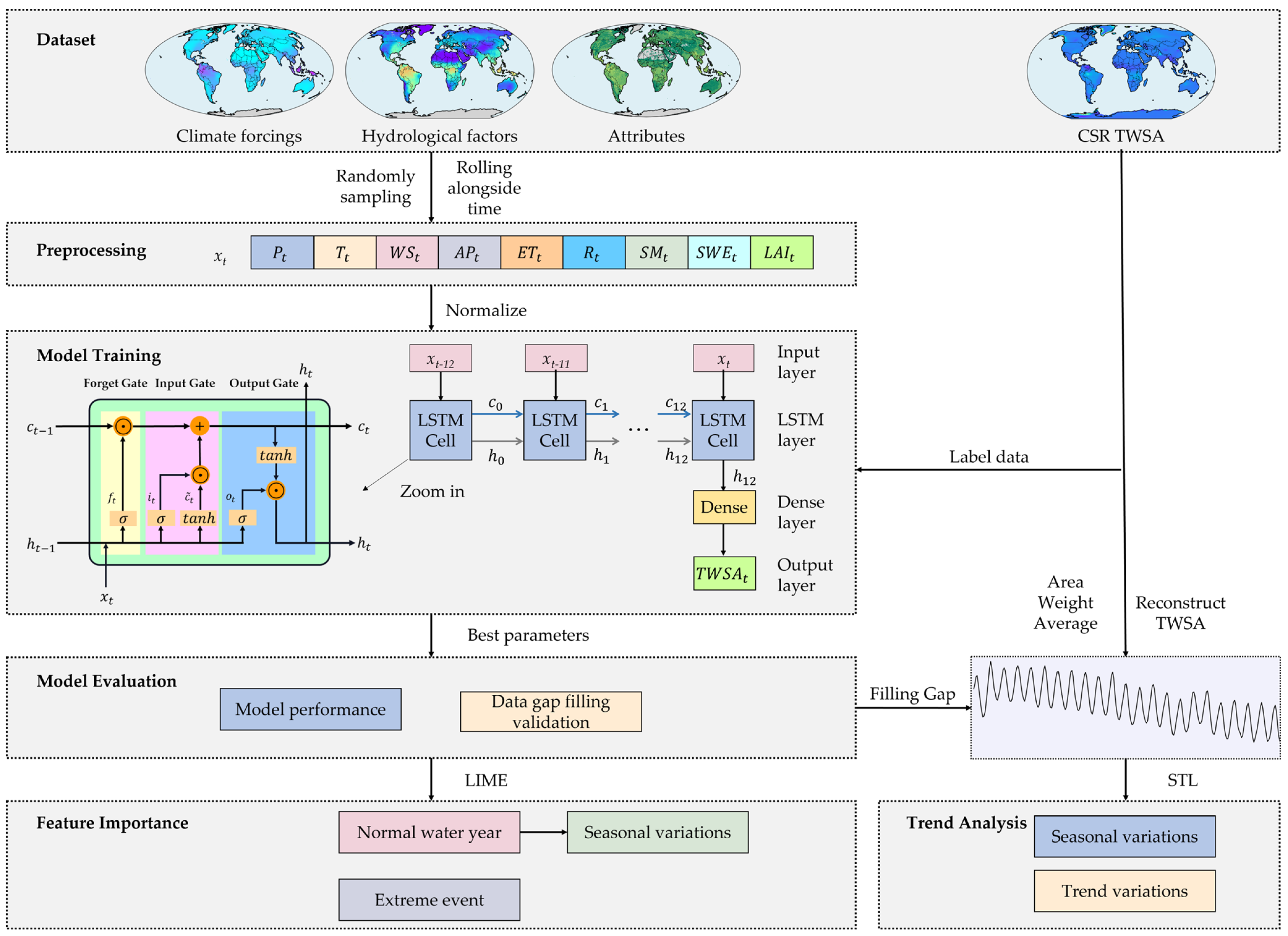
The LSTM architecture comprised an input dense layer (256 neurons), three consecutive LSTM layers (each with 256 neurons), and an output dense layer (1 neuron for TWSA prediction). Input data were carefully aligned spatially; a minor discrepancy of 8.37% exists between the effective global land grids used and the official CSR land mask (Figure S1). The dataset covered 22 years (April 2002 to March 2024). It was randomly split into training (70%), validation (15%), and testing (15%) sets based on time steps. A collinearity test using the variance inflation factor (VIF) showed low multicollinearity among input features (Table S1), supporting the reliability of driver analysis. The model was trained to minimize the mean squared error (MSE) loss function using the Adam optimizer [56]. Training converged over 20 epochs in approximately one hour using two NVIDIA RTX A6000 GPUs. The LSTM model was implemented using the TensorFlow framework (version 2.11.0).
To comprehensively evaluate model performance and assess its spatial and temporal recognition ability, four metrics including correlation coefficient (CC), Nash–Sutcliffe efficiency (NSE), normalized root-mean-square error (NRMSE) and BIAS are included. CC and NRMSE indicate the total correlation and absolute deviation between the prediction and observation, respectively. NSE represents the total performance of fitting, and BIAS measures how much the model underestimates or overestimates TWSA. Combinations of above four metrics are considered to be more balanced. The equations can be found in the Supplementary Materials. The complete technical workflow is shown in Figure 1.
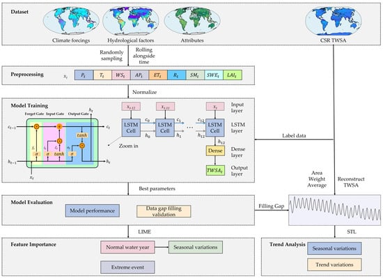
Figure 1.
Flowchart illustrating the LSTM-based methodology for reconstructing and interpreting TWSA dynamics.
2.3. LIME
LIME is an artificial intelligence technique for local post hoc explanation based on surrogate theory [42]. It effectively elucidates the predictions made by any classifier or regressor by approximating it locally with interpretable models, such as linear models. Different to other approaches like SHAP, LIME provides intuitive interpretations with high local fidelity, ensuring that explanations for individual predictions should at least be locally faithful. In this context, variations of model outputs at a local scale can be conceptualized as a linear system and captured by linear combination of features, which can be simplified as the following equation:
where x is the instance to interpret, g is a surrogate linear model created by LIME, and f is the pretrained model. Ω(g) represents the number of non-zero weights, and πx denotes a proximity measure defined locality around x. Thus, to ensure both interpretability and local fidelity, L(f, g, πx) has to be minimized while keeping Ω(g) sufficiently low. Further, in this study, the local effect of driving factors was assumed to be linear, and each grid was explained separately to discern the spatial pattern of the importance of driving factors. This approach effectively maintains local fidelity and balances explanation granularity and computational efficiency, crucial for interpreting model predictions. To capture seasonal variations and reduce computational costs, three normal water years (2004, 2009, and 2016) were selected, with four representative months (January, April, July, and October) from each year. Additionally, four extreme event months were included in the analysis: an extremely dry month (February 2023), an extremely wet month (July 2010), a low-temperature month (January 2011), and an extremely high-temperature month (July 2018). To further reduce computational costs, a 4 × 4 moving window was applied to sample global grid points spatially for each month to explain. For normal months, the grid point with the multi-year average of TWSA value closest to the window’s mean was selected for explanation. For extreme event months, the grid point with the largest variance across multiple years was chosen.
2.4. Temporal Variation Analysis
The primary TWSA series and driving factor dynamics derived from GRACE and Noah data capture the monthly variations of TWS and its driving factors within the Earth’s climate system. However, these primary signals encompass multiple components, such as seasonal signal, and it is necessary to isolate single components by removing other components to accurately investigate variations at specific scales. For instance, the trend component should be extracted from the primary TWSA time series to discern the effects of climate variability and human activity. Here, seasonal-trend decomposition based on loess (STL) method is adopted to decompose time series into trend, seasonal, and residual components, which is a robust and versatile method proposed by Cleveland et al. [57]. This method relies on local regression smoothing, where an inner loop is nested within an outer loop. The STL procedure involves multiple applications of loess smoothing, allowing analysis of procedural properties, fast calculations for long-term time series, and strong smoothing of trends and seasonal variability.
The method has been widely used to decompose GRACE TWSA when analyzing the different time series components. The capability of STL for disaggregating the original GRACE TWSA has been demonstrated by Humphrey et al. [58]. Here, we employ STL to decompose the monthly TWSA time series derived from GRACE and GLDAS as shown in the following formula:
where the long-term component (Slong-term), seasonal component (Sseasonal), and residual component (Sresidual) reflect the low-frequency signal, seasonal signal, and sub-seasonal signal combined with noise, respectively.
To analyze the temporal evolving of TWS across years, TWSA trends—represented by linear trends—are estimated through least squares regression applied to the long-term (deseasonalized) TWSA after STL analysis. This estimation is further validated using the Mann–Kendall trend test (MK test), which is widely used to detect trends in hydrologic data [59]. The MK test is a non-parametric and robust test for identifying the trend in a time series [60]. The MK test in this study is implemented by using the original Mann–Kendall test from the pyMannKendall package (version 1.4.3) in Python 3.11.11 [61], which does not consider serial correlation or seasonal effects. Global mean TWSA and TWSC values are computed using area-weighted averaging to account for latitudinal differences in grid cell size. Moreover, monthly changes of TWS, referred as TWSC, were estimated by the double-difference time derivative of TWSA instead of the simple difference derivation, which provides smoothing effects [62,63]. The simple difference derivation represents TWSC from the mean value of TWSC over a half-month period (such as TWSC from the month t to the middle of month t and month t + 1), which is different from temporal resolution of monthly and may introduce larger errors than double difference derivation [64,65]. Therefore, monthly TWSC can be estimated as follows:
where TWSCt is TWSC for month t; TWSAt+1 and TWSAt−1 represent TWSA for month t + 1 and t − 1, respectively; and Δt denotes the time interval between adjacent measurements, one month here for continuous data.
3. Results
3.1. Model Performance
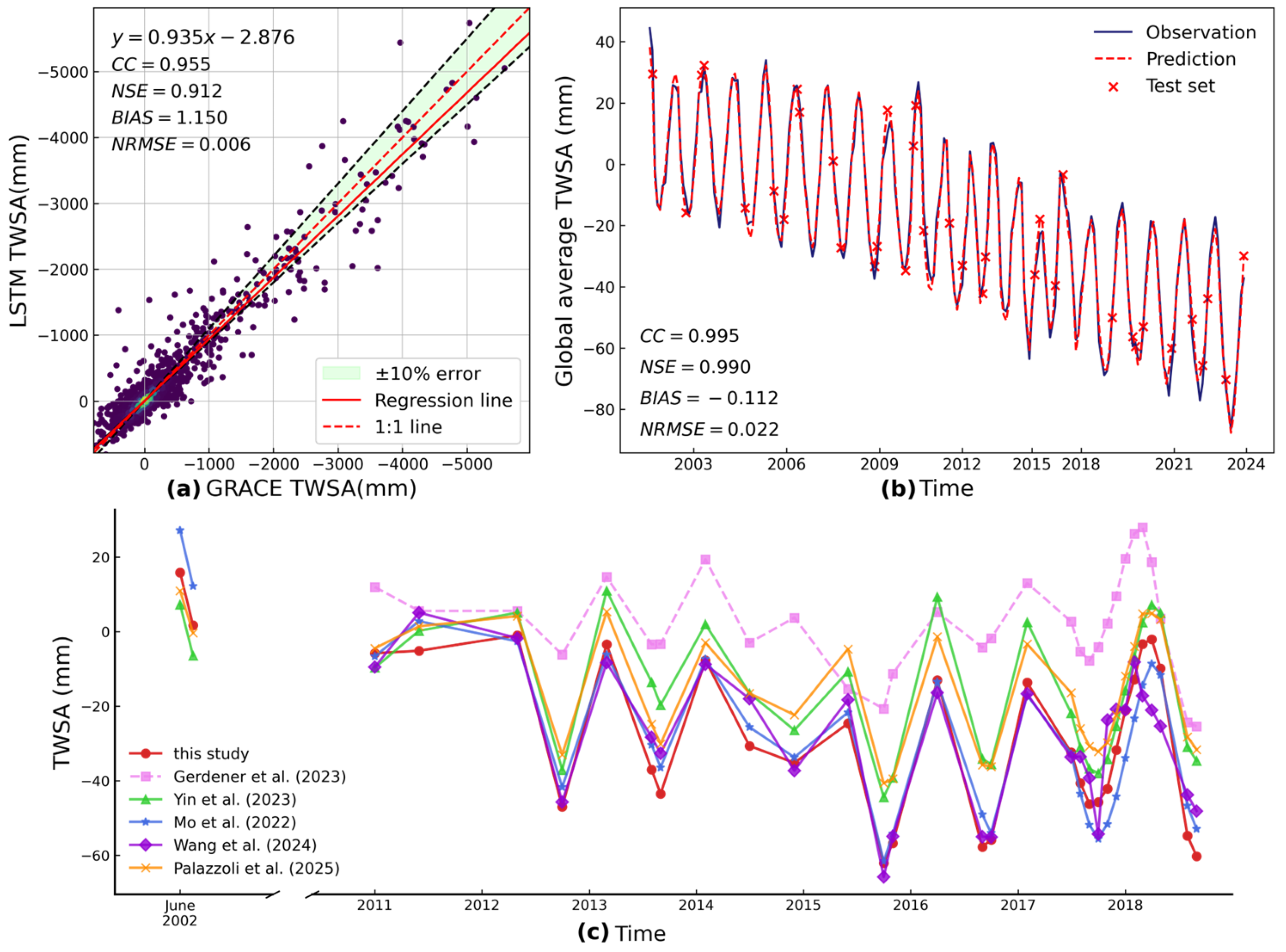
To comprehensively evaluate model performance which is closely related to the reliability of the model interpretation, a rigorous assessment was conducted. The prediction accuracy was examined using the testing set of the GRACE data (36 months) with four metrics. Figure 2a shows a density scatter plot comparing LSTM-predicted TWSA against GRACE observations, demonstrating strong agreement (CC = 0.955, NSE = 0.912, BIAS = 1.150 mm, NRMSE = 0.006 mm). Figure 2b illustrates the temporal performance of the LSTM model from 2002 to 2024. Generally, the LSTM model exhibited an excellent capability in capturing the temporal variations of TWSA, achieving a CC of 0.995 and an NSE of 0.990, along with a BIAS of −0.112 mm and a NRMSE of 0.022 mm. However, the LSTM model occasionally struggled to reproduce extreme values, particularly in early and recent years such as 2002, 2021, and 2023, where it predicted more typical values instead.
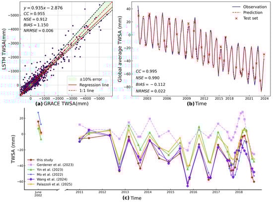
Figure 2.
(a) Density scatter plot between observations and simulations on the test set (displaying a subset of samples, specifically 10,000 points); (b) comparison of the global average TWSA time series derived from GRACE and LSTM from April 2002 to March 2024; (c) comparison of data gap filling results with previous studies (dashed lines indicate hydrological models; solid lines represent data-driven models) [35,36,38,40,41]. Note that reconstructions by Palazzoli et al. [41] exclude Greenland.
To assess the reliability of our gap-filling results, we compared our reconstructed data with several previously developed reconstruction products [35,36,38,40,41]. Results show that the five machine learning or deep learning-based products exhibit strong consistency, supporting the robustness of our approach. In contrast, the GLWS2.0 product [35], which is based on a hydrological model, shows notable discrepancies with machine learning productions. Notably, the model developed by Mo et al. [38] was widely regarded as one of the most accurate at the time of its publication, while the models proposed by Wang and Zhang [40] and Palazzoli et al. [41] represent the most up-to-date approaches. The close agreement between our results and those of both Wang and Zhang [40] and Palazzoli et al. [41] further demonstrates the high accuracy of our reconstruction.
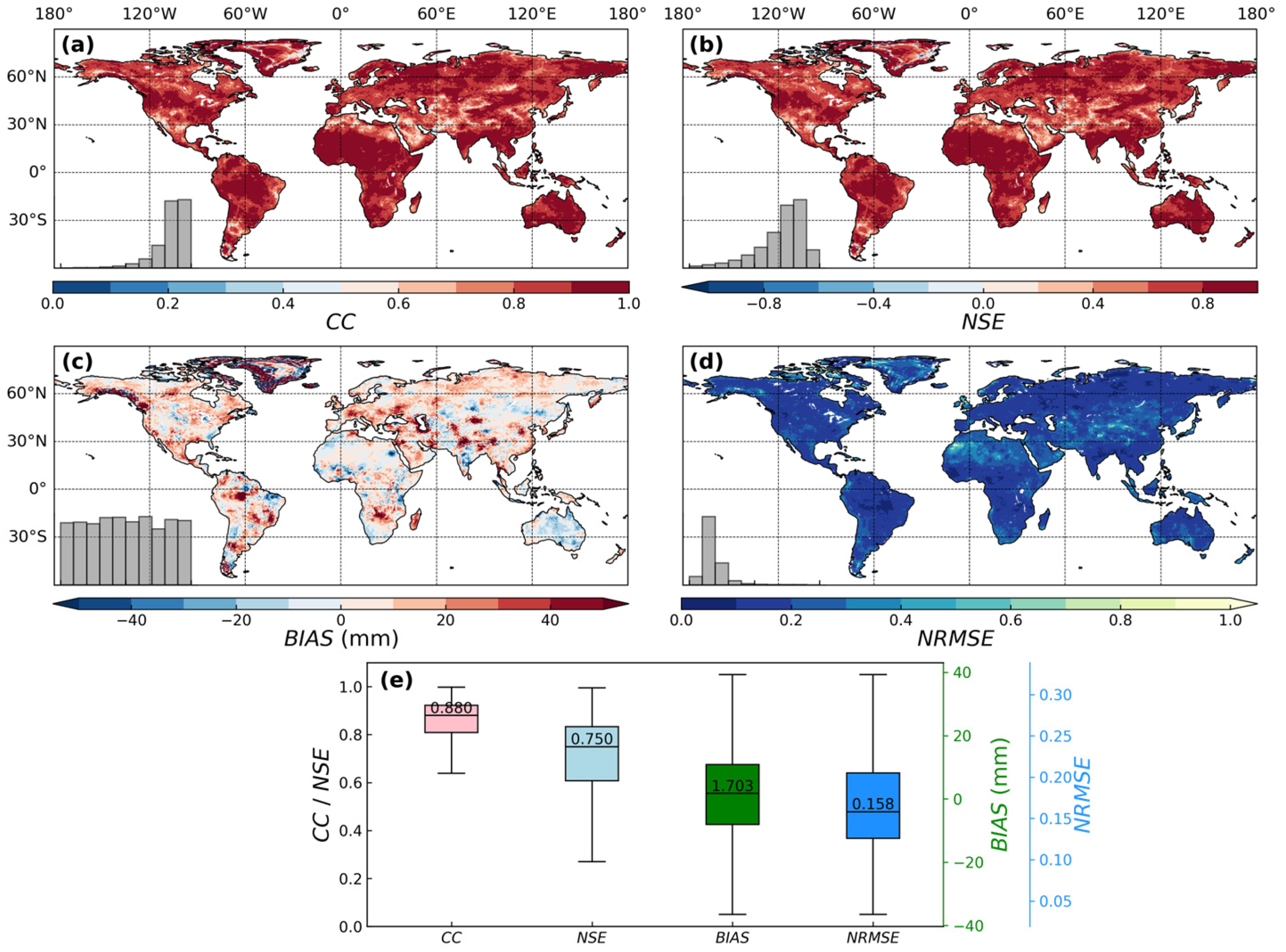
The model’s pixel-wise performance on the test set is presented in Figure 3. Evaluation yielded a median CC of 0.880, a median NSE of 0.750, a BIAS of 1.703 mm, and an NRMSE of 0.158 mm, reflecting lower skill compared to the metrics achieved in the temporal performance analysis. Generally, the model tends to fit the data relatively well for the humid zones, such as most of the lower- and middle-latitude regions with a higher CC and NSE, while it performs relatively poorly for arid zones like the Middle East. The model also showed limitations in capturing extreme TWSA values accurately. Notably, regions such as central Greenland and areas near the 30°N and 30°S latitudes, including northwestern Australia and the Middle East, exhibited poorer agreement with observations, reflected in relatively low CC and NSE values and higher BIAS and NRMSE. Furthermore, the model exhibited biases in Greenland, with overestimation in peripheral areas and underestimation in the central ice sheet. This suggests that the model may struggle to accurately capture the complex ice dynamics of TWSA in Greenland and its surrounding areas, despite the inclusion of SWE data as an input. Nevertheless, the LSTM model demonstrates acceptable performance across most global land areas, achieving generally high correlation and goodness-of-fit. This level of performance supports the feasibility of and provides confidence in subsequent interpretations of driver importance using LIME.
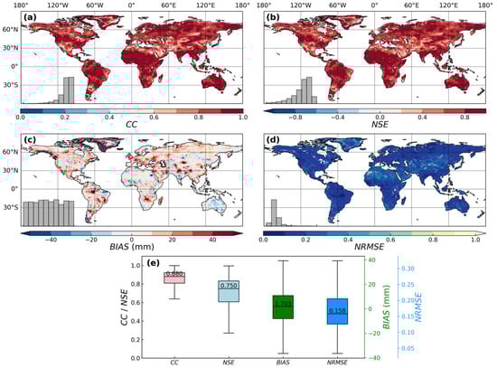
Figure 3.
Spatial distributions and box plot of performance metrics with inset subplots showing the frequency distribution of each metric (using the same range as the color bar). CC (a), NSE (b), BIAS (c), NRMSE (d) and box plot of the four metrics calculated from LSTM simulated against GRACE observed TWSA. The box plot (e) summarizes these four metrics based only on the grids in the testing set.
3.2. Trend Analysis and Seasonal Variations
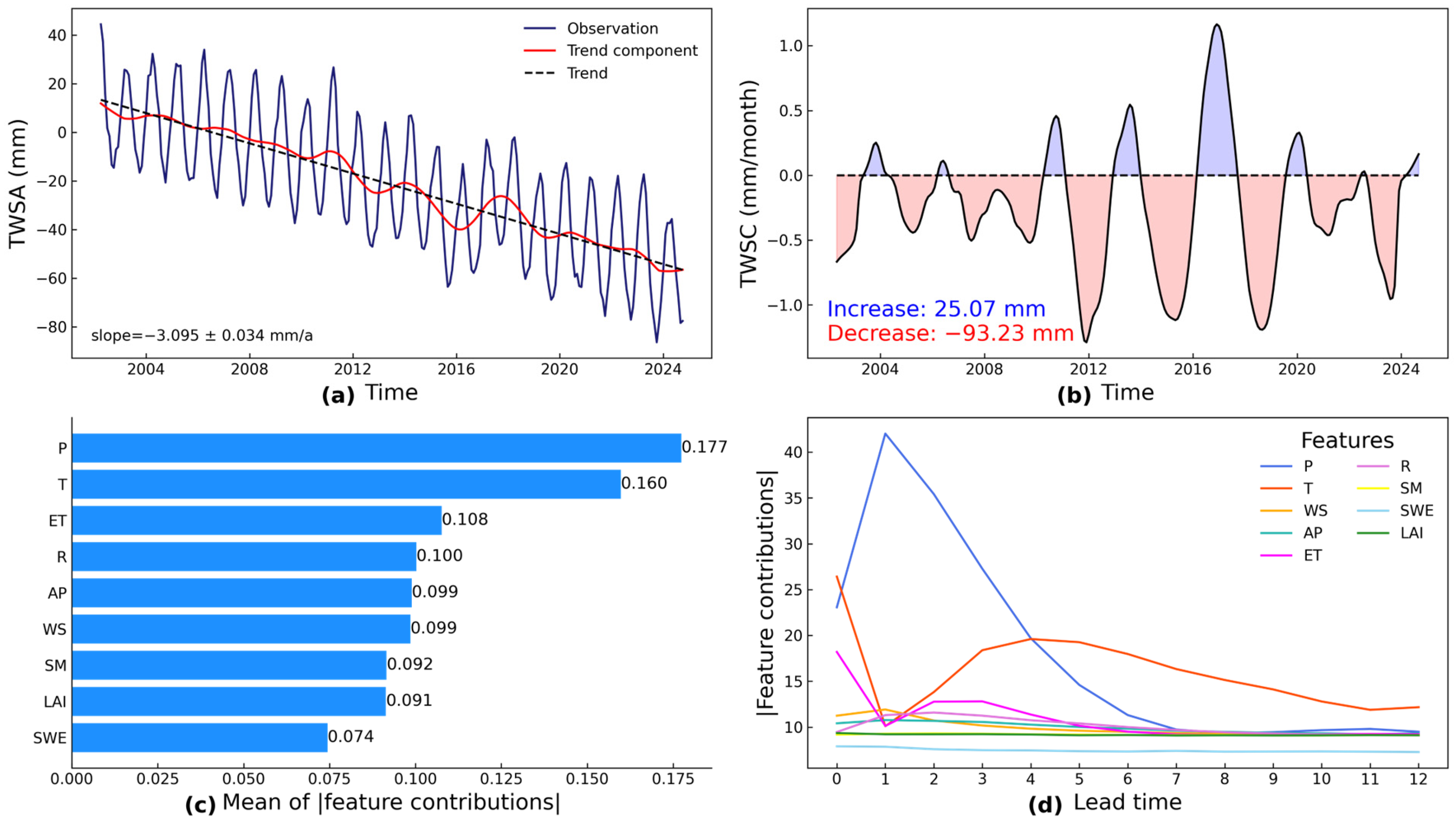
Figure 4a presents the dynamics of global average TWSA, with the 33 months of missing data imputed by the LSTM model. The GRACE TWSA dynamics were decomposed into long-term trend, seasonality signal, and residual signal using the STL analysis to facilitate the examination of inter-annual variations. Figure 4a depicts the inter-annual variations of TWSA and its trend component from 2002 to 2024. Generally, the global mean TWSA shows a significant decreasing trend of −3.095 ± 0.034 mm/a (p < 0.001) (Antarctica excluded in all subsequent calculations), amounting to a cumulative decline of approximately 70 mm over the 22-year period. Figure 4b illustrates the inter-annual variations of TWSC, highlighting a prevailing downward trend across most years, with notable decreases in 2012, 2015, and 2019, punctuated by significant increases in 2011, 2013, and 2017.
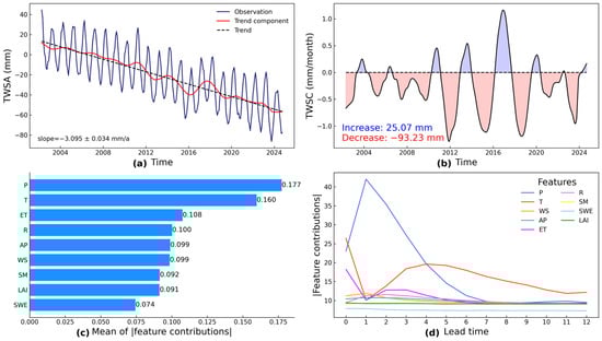
Figure 4.
Dynamics of TWSA (a) and TWSC (b) from 2002 to 2024, the ranking of feature importance (c) and the contributions of different features across various lead times (d), based on LIME.
To further explore the underlying mechanisms driving these trends, we interpreted the LSTM model’s predictions using LIME to analyze the importance of the input driving factors, illustrated in Figure 4c,d. Our findings underscore that precipitation and temperature exert the dominant influence on global mean TWSA. Other meteorological factors, including evapotranspiration, runoff, surface air pressure, wind speed, and soil moisture, alongside LAI and SWE, play less significant roles globally. Figure 4d shows the variations of feature importance relative to the prediction time (lead time), revealing two different patterns aligned with their respective hydrological timescales. Factors characterized by shorter response times exhibit non-linear importance dynamics, often accompanied by multiple extremes. For instance, the impact of evapotranspiration and its main driver temperature reaches a peak at lead time zero (current month), then recedes before rising sharply, hitting a second extreme three to four months prior; this secondary peak may be associated with delayed responses such as plant transpiration or seasonal energy storage impacting ET rates with longer time scales. For factors with longer response times, such as runoff, wind speed, and precipitation, they show heightened importance at short lead times and diminishes over longer lead times, hitting extremes with a lead time of approximately one to two months. In particular, precipitation exerts its peak importance with a lead time of one month, while the importance of runoff peaks two months prior, which may reflect the combined effects and travel times of the baseflow and snowmelt runoff. For factors with lesser importance in the global average, such as SWE and SM, their significance shows only slight fluctuations, and the temporal variation in importance is not significant. This low global average importance may be attributed partly to the model not assigning sufficient weight to these factors globally, or their impacts being more localized.
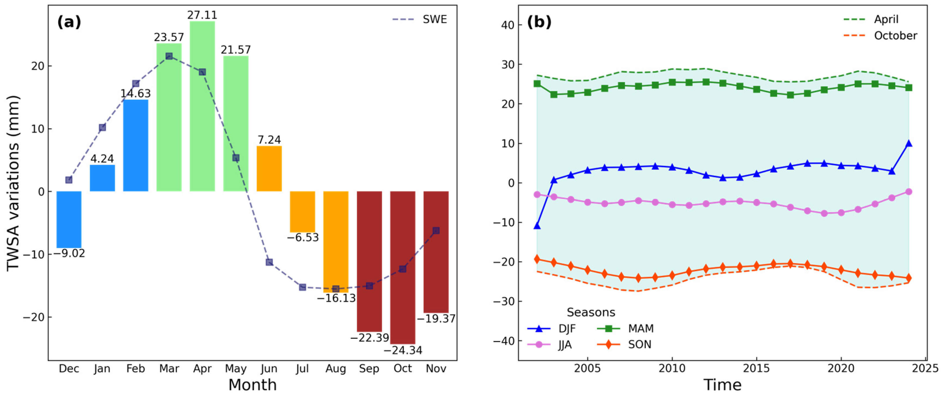
The seasonal variations in global mean TWSA are shown in Figure 5. Global mean TWSA shows significant growth from March to May, peaking at 27.11 mm in April, and experiences a sharp decline from July to October, reaching a minimum of −24.34 mm in October. This pattern is similar to the variation of SWE (dashed line in Figure 5a), with a lag time of approximately one month. This lag is likely driven by the time required for snowmelt (which peaks from March to May in the Northern Hemisphere, which encompasses more than 70% of the total terrestrial area and from September to November in the Southern Hemisphere) to contribute to TWS components. During these periods, as temperature rises, ice and snow begin to melt and transform into runoff and soil moisture, with a portion flowing into lakes or oceans. Simultaneously, a large amount of water evaporates and transpires back to the atmosphere, leading to the decrease in land TWS, culminating in the tipping point before summer. Moreover, the inter-annual variations of TWS in MAM (maximum in April) and DJF increase slightly across the 22 years, while TWS in SON shows a slightly decreasing trend.
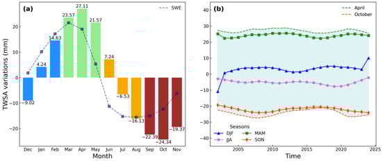
Figure 5.
Monthly climatology (a), and seasonal variations (b), of global mean TWSA. DJF refers to December through February, MAM to March through May, JJA to June through August, and SON to September through November.
3.3. Spatial Patterns of TWSA Trends and Drivers
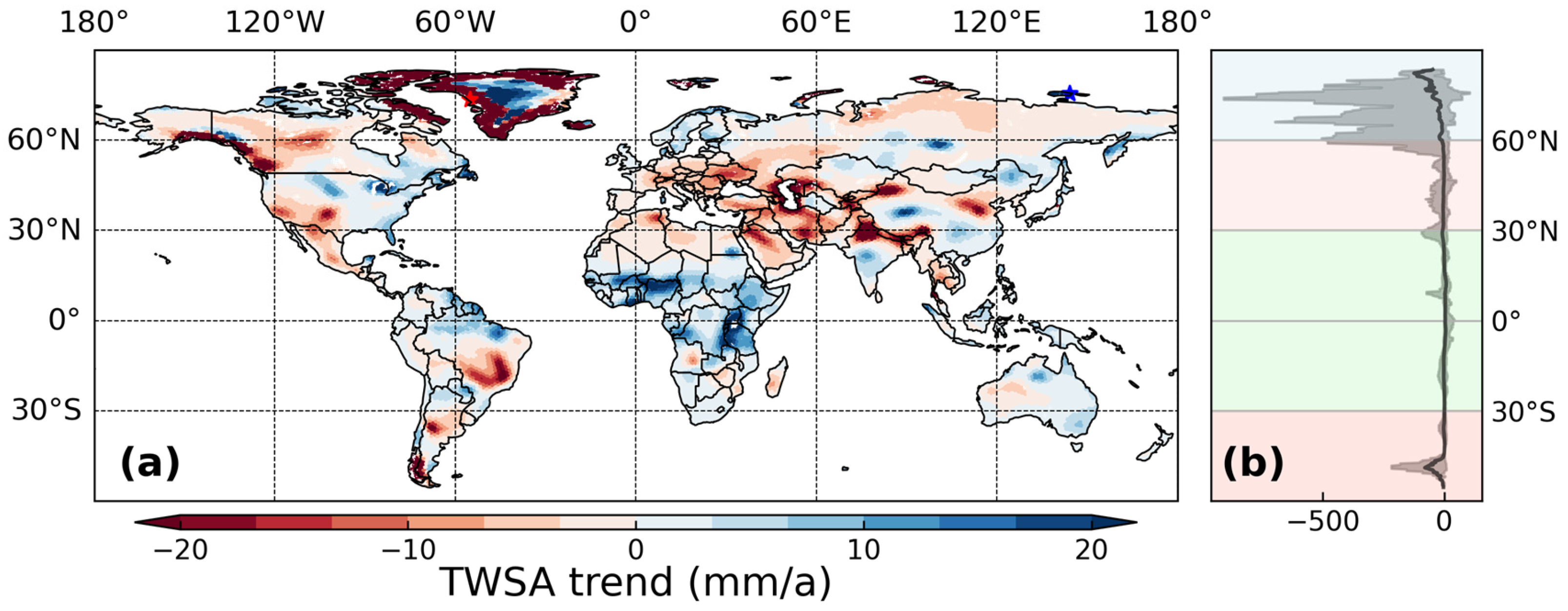
Figure 6 maps the spatial distribution of the TWSA trends over the 2002–2024 period. Significant spatial heterogeneity is evident, with red areas indicating declining TWSA (deeper red signifies larger loss rates) and blue areas indicating increasing TWSA. We found that trends in TWS vary significantly across latitudes. High-latitude regions contribute the most to global TWS reductions, with notable declines in Greenland’s peripheral regions, the Gulf of Alaska coast, and the Canadian Archipelago. Among these regions, Greenland makes the largest contribution, with sharp decreases in its peripheral areas reaching nearly 900 mm/a, whereas its central region shows an increasing trend, with a maximum of 50 mm/a. These high-latitude declines, particularly the mass loss from glaciers and ice sheets like Greenland’s, are the primary drivers of the overall negative trend in global mean TWSA. Mid-latitude regions also experience considerable TWS losses. Most mid-latitude regions exhibit a declining trend, except for the eastern United States, whereas low-latitude regions generally show an increasing trend, with central Brazil as an exception.
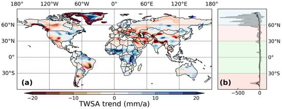
Figure 6.
The spatial pattern of TWSA trend at pixelwise (a) and the TWSA trend across latitudes (b). Marker star in figure (a) marks the maximum increase trend using blue color and minimum decrease trend using red color; the grey area in figure (b) represents the range of TWSA trend and the black line marks the average trend, with different colors representing different latitudes.
To further explain the drivers behind these spatially varying changes, an analysis of factor importance at each grid point was conducted based on the LIME method (Figure 7). The results indicate that precipitation is the dominant driver in most low-latitude and mid-latitude humid regions, as well as in certain arid areas such as Northern Africa and the Middle East, where rainfall variability strongly impacts sparse water resources. Temperature, on the other hand, plays a more important role in arid regions and in areas covered by ice or snow. In these cryosphere regions, snow-related variables, such as snowmelt-influenced runoff and SWE, exert a stronger influence on TWSA dynamics than in other regions. In mid-latitude regions, TWSA changes are often driven by the combined effects of multiple factors. Among the other contributing factors beyond precipitation and temperature, air pressure exerts a particularly significant influence in mountainous areas, while evapotranspiration, runoff, wind speed, and soil moisture also contribute to variability.
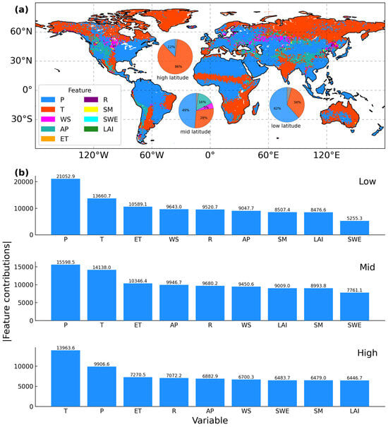
Figure 7.
The spatial pattern of the dominant driving factors of TWSA over three normal water years at pixelwise (a) and histogram of dominant driving factors across different latitudes (b). The inset pie chart in subgraph (a) illustrates the proportion of driving factors across latitudes.
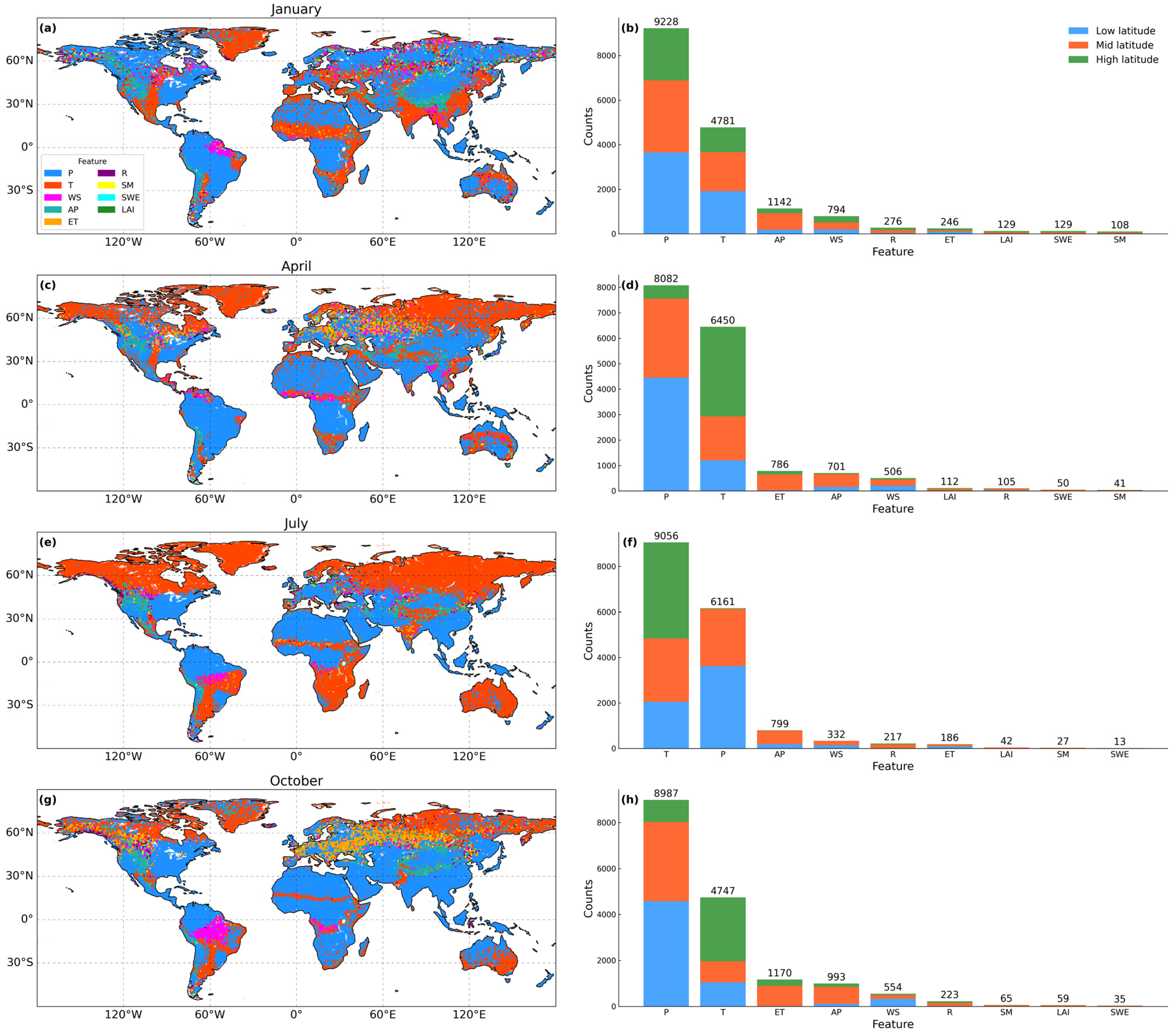
Figure 8 illustrates the spatial patterns of factor importance across different seasons. On a global scale, although the relative rank of the driving factors shows little temporal variation, their spatial distribution varies markedly seasonally, particularly in mid-latitude regions. From January to July (Northern Hemisphere winter to summer), as temperature and precipitation increase, the influence of precipitation gradually diminishes, particularly at mid to high latitudes. In contrast, temperature-controlled areas expand, and its influence on high-latitude and high-altitude regions (e.g., the Tibetan Plateau) rapidly increases. Meanwhile, the influence of evapotranspiration initially strengthens before decreasing. From July to January, however, these trends reverse. Additionally, factors beyond temperature and precipitation are primarily active in mid-latitude regions. Runoff is most prominent in January and July, corresponding to snowmelt runoff and surface runoff, respectively. Air pressure has a greater impact during colder months, sometimes competing with temperature for dominance, while the effects of soil moisture and SWE are primarily evident in winter.
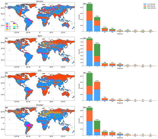
Figure 8.
Seasonal variations in dominant TWSA driving factors identified by LIME. Left: Spatial maps representing the dominant factor at the pixel level for representative months: January (a), April (c), July (e), October (g). Right: Histograms illustrating the global percentage of land area dominated by each factor in the corresponding month: January (b), April (d), July (f), October (h).
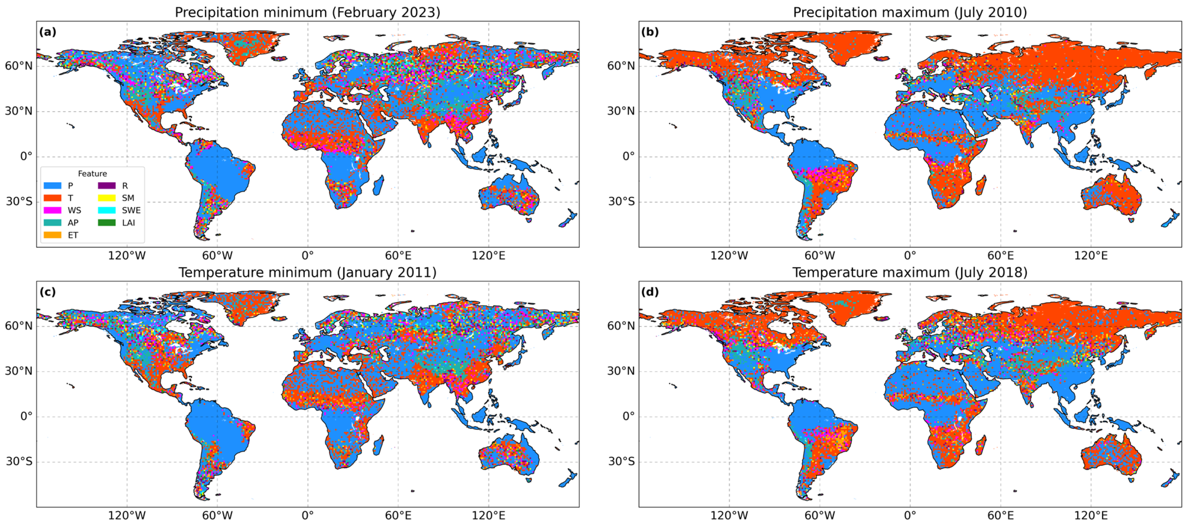
Figure 9 illustrates how the spatial patterns of dominant TWSA driving factors shift during selected extreme weather months. The analysis suggests that the spatial responses of dominant drivers during extreme precipitation events and extreme temperature events can exhibit similarities. The spatial distribution of dominant drivers when precipitation reaches its minimum (e.g., during drought) appears similar to that when temperature reaches its minimum (cold extremes), especially at low latitudes. The same pattern holds true for maximum precipitation (wet extremes) and maximum temperature (heat extremes). This can be partially attributed to the coincidence of rain and heat. For instance, when the temperature reaches its minimum (represented by January 2011), the relative influence of both temperature and precipitation is smaller compared to a typical January, with a significant increase in the relative influence of SWE, soil moisture, and wind speed in mid- to high-latitude regions. Interestingly, when temperature reaches its maximum (represented by July 2018), compared to wet extremes, temperature-dominated regions remain largely unchanged in spatial extent and the dominance of temperature may even slightly decrease in some areas, potentially due to co-limitation by water availability.
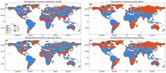
Figure 9.
Spatial distributions of dominant TWSA driving factors across four extreme event months: precipitation minimum (a), precipitation maximum (b), temperature minimum (c), and temperature maximum (d).
4. Discussion
4.1. Impact of Driving Factors on TWS
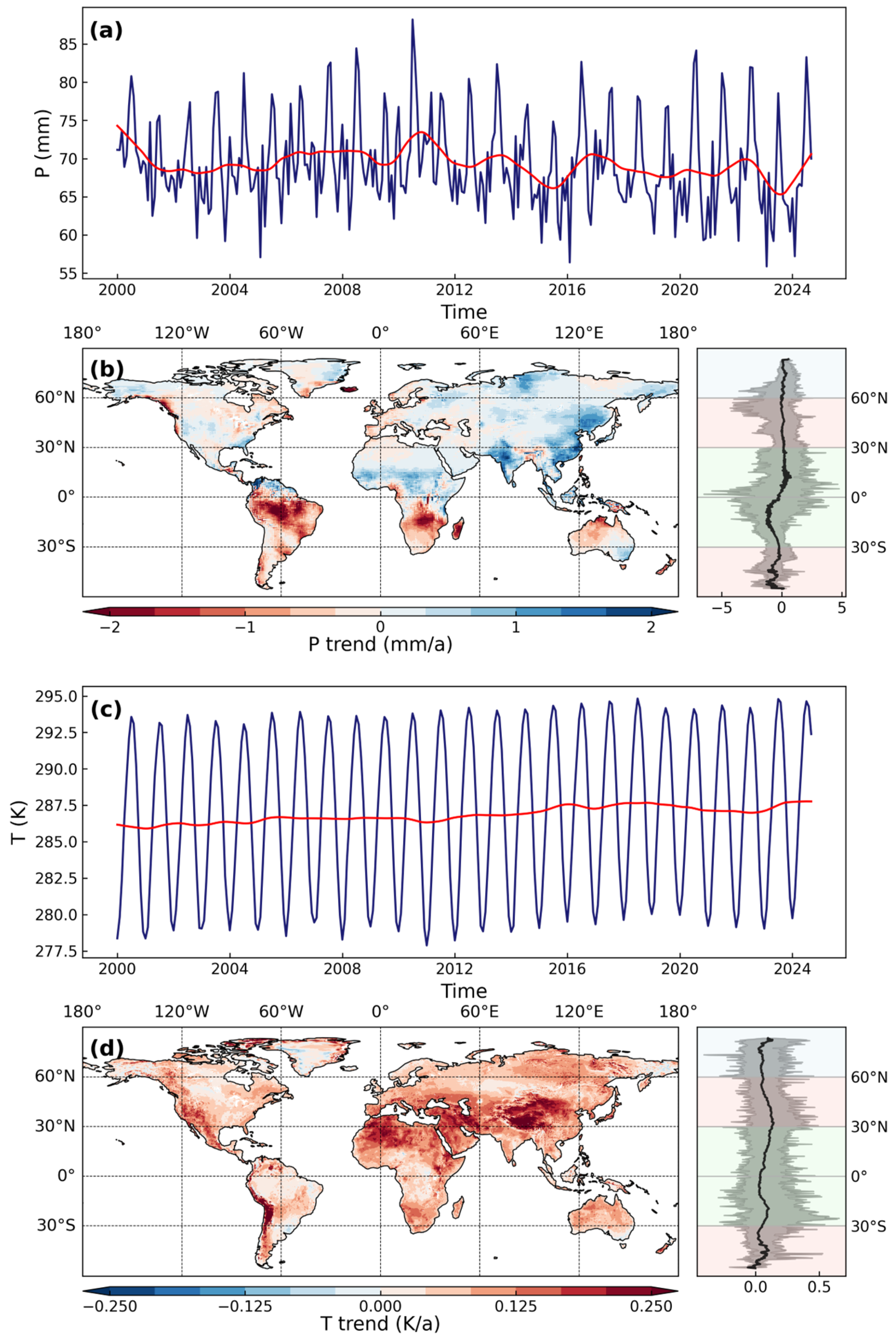
Over the course of two decades, the decrease in the global average of TWS is closely linked to ongoing climate change. During the 22-year period, as the leading driving factor identified by LIME for the global mean, monthly precipitation exhibits seasonal fluctuations and a slight decreasing trend (p < 0.001) in the global averages (Figure 10).
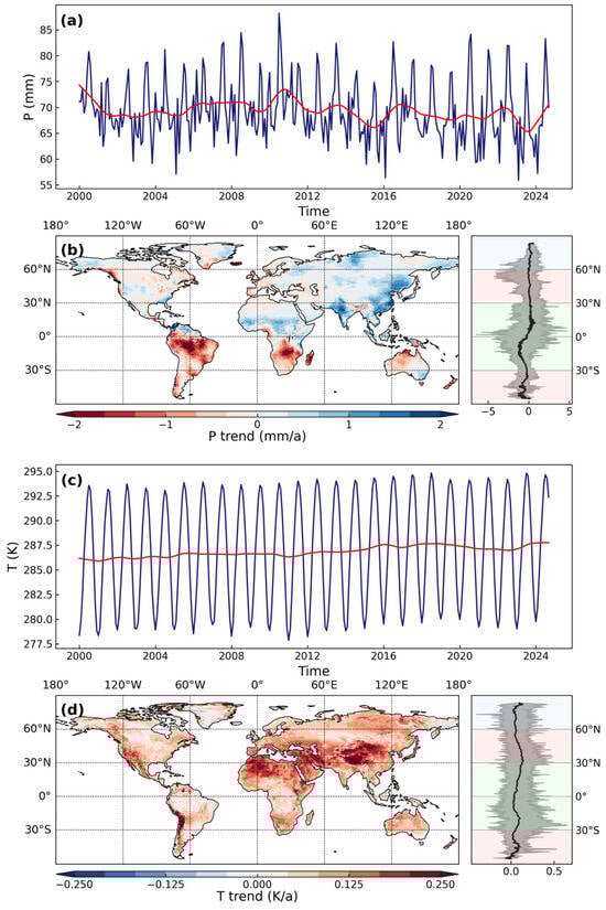
Figure 10.
Global average dynamics and spatial distribution of trends for precipitation (a,b) and temperature (c,d) at the pixel level. Panels (a,c) display the global mean TWSA time series with STL-derived trend components overlaid in red. Panels (b,d) present the corresponding spatial trend maps, accompanied by latitudinal profiles on the right (black lines indicate the mean trend across longitude, and shaded areas represent the range).
Significant variability in precipitation was noted in low-latitude regions such as South America and the Pacific coasts, with an increase in northern latitudes and a decrease in southern latitudes globally. Additionally, its influence on TWS fluctuates non-linearly over time, initially increasing and then decreasing, with a lag time of approximately one month corresponding to the maximum influence (Figure 4d). Temperature exhibits a prevailing ascending trend (~0.01 °C/a), with more pronounced changes observed in the Tibetan Plateau, northern Africa, and the Middle East, where most of the notable variations in TWS are observed. The LIME analysis reveals distinct temporal patterns in driver importance (Figure 4d). Temperature, a primary driver of both ET and snowmelt, exhibits an importance pattern similar to that of ET, featuring a peak at lead time zero (current month) and a second, delayed peak three to four months prior. This likely reflects temperature’s immediate influence on ET rates and potentially lagged effects related to seasonal energy storage or vegetation cycles influencing water availability. In contrast, drivers like precipitation and runoff show maximum importance with a one to two month lag, reflecting the time needed for these fluxes to significantly impact storage. These different temporal importance patterns revealed by LIME correspond to the varying timescales and complexities of the underlying hydrological processes (e.g., rapid ET response vs slower infiltration and runoff generation) that govern how climate forcings ultimately translate into changes in TWS. Additionally, these effective response lags identified by LIME vary across regions, generally shorter in low-latitude basins and more prolonged in high-latitude areas [66,67,68]. ET displays a slight ascending trend (slope = 0.014 mm/a, p < 0.001) during 2000 to 2024. Spatially, an increase was observed in North America and northern South America, while a decline occurred in southern South America. Runoff and soil moisture show a slight declining tendency, whereas wind speed and surface pressure showed no discernible patterns (Figures S2–S7).
Although total water storage remains conserved on a global scale, there is a redistribution of water and energy between land and oceans (Figure S8), which is a primary direct cause of TWS loss. TWS has consistently experienced a marked decline from 2002 to 2024, accompanied by a notable increase in oceanic liquid water equivalents (Figure S8c), evident in the observed sea level rise in recent years. This may also explain why many regions experiencing significant TWS changes are located along coastlines or near large lakes. Further, reductions in TWS are primarily observed in ice- and snow-covered regions, such as the high-latitude regions. This aligns with the similar annual variation patterns between TWSA and SWE, suggesting the important role of SWE in long-term TWSA changes. However, in the analysis of driver importance, SWE does not show a large contribution even in high-latitude regions. We believe the reason for this phenomenon is twofold. On one hand, the snow data from ERA5-Land may not accurately represent the actual snow and ice conditions, particularly ice sheet dynamics, with almost no changes shown in the ice and snow fields in Greenland (Figure S4). This may also explain the large BIAS observed near Greenland. On the other hand, temperature is also a contributing factor. Temperature, which is the main driver of SWE variation, has the largest contribution according to LIME in high-latitude regions, especially in July. In these regions, spatial patterns of TWS variations are also similar to that of temperature. As global warming accelerates the loss of ice and snow, it drives glacier retreat and increases snowmelt runoff from land to oceans, ultimately leading to a decline in TWS. As for autumn and winter, although the total precipitation amount is relatively low, the proportion of snowfall is significantly higher, and losses from runoff and evaporation are minimal. As a result, most of the precipitation effectively contributes to replenishing TWS. Consequently, precipitation becomes the dominant factor influencing TWS in high-latitude regions by January. In particular, Figure 5b suggests that TWSA in DJF has increased in recent years.
The temporal and spatial patterns in mid-latitude regions are more diverse where human activities are frequent, and natural processes are complex, with multiple factors playing a role. In details, the main losses in TWS are observed in the coasts of the Mediterranean Sea, Caspian Sea, Black Sea, Tibetan Plateau, and Gulf of Alaska. These regions are characterized by their proximity to large water bodies and significant temperature fluctuations. In these regions, temperature and precipitation generally dominate, while other factors such as evapotranspiration, air pressure, and runoff also play a significant role seasonally. For example, air pressure has its strongest influence in mountainous areas, while ET exerts an effect mainly in April and October. This complexity may help explain why the decrease in TWS and the variations in factor importance under changing environmental conditions are less pronounced in mid-latitudes than in high latitudes. Compared to previous research, our results further suggest that precipitation, as well as temperature, may play a larger role than we expected. Nevertheless, the model’s recognition of the impact of human activities is relatively limited. For instance, in the North China Plain, TWS loss is primarily attributed to excessive groundwater extraction. In low-latitude regions, the TWS is mainly dominated by precipitation and its patterns closely aligning with spatial precipitation patterns. Additionally, combined with the interpretation results for extreme temperatures, the results indicate that climate change will continue to have a more pronounced impact on TWS in high-latitudes in the short term, with a relatively weaker impact on TWS at mid- and low latitudes.
4.2. Limitations and Future Prospects
This study highlights two issues, however. First, in recent years, TWS dynamics have been significantly impacted by both human activities and climate change. The increasing intensity of human activities has gradually amplified their impacts on TWS, sometimes even surpassing the influence of natural processes in certain regions [64]. For example, water withdrawals significantly influence TWS. Huang et al. [69] reported that globally, the majority of water withdrawal is used for irrigation, primarily concentrated in regions with extensive irrigated croplands and high agricultural production—such as the western United States, eastern China, and India. The corresponding reductions in TWS caused by these withdrawals have also been captured by GRACE satellite observations (Figure 6). However, this study assessed the intensity of human activities through the land attribute—specifically LAI data—instead of explicitly incorporating human activity data to accurately characterize their impacts. This limits the ability to accurately quantify the impacts of human activities. Moreover, the absence of explicit human influence data may lead to biased or even incorrect attribution of the primary drivers of TWS changes in this study, particularly in densely populated regions. Climate change also exerts a considerable impact on the TWS. For example, there was a sharp increase in global mean TWS in 2017, along with large variability (alternating increases and decreases) before and after that year, possibly related to ENSO events (Figure 4b) [70]. Larger-scale climate impacts, however, require longer time series to be fully understood.
Second, this study analyzed the driving factors of TWS on a global scale using the LSTM model and LIME. The effectiveness of this method is closely tied to the accuracy of the DL models and the reliability of interpretation techniques, which are highly dependent on the quality of the input data. On one hand, certain processes still lack high-precision monitoring data suitable for global modeling, such as snow and ice dynamics, which may be the reason for observed model inaccuracies and potential limitations in driver attribution. On the other hand, the black-box nature of deep learning models and the difficulty in quantifying uncertainty introduce challenges in assessing model reliability and understanding represented processes. However, the integration of physics into DL models holds great potential in addressing this issue.
It is important to consider the potential impact of land–ocean signal leakage on the conclusions of this study. Although the CSR RLv06.3 product employs refined processing of boundary grids and corrections to gravity anomalies to reduce coastal signal leakage, and although deep learning models have some capability to correct systematic biases, such leakage remains a non-negligible source of error. Specifically, static systematic biases may introduce deviations in TWSA estimates in coastal and lakeside regions. While these deviations may have limited influence on long-term trends in many such areas, they could be more pronounced in certain regions—particularly in high-latitude zones or densely populated regions. In these regions, climate change or human activities may cause glacier retreat or shrinking lake surfaces, leading to shifts in land–water boundaries. These boundary changes may bias both the estimation of TWSA trends and the attribution of their driving factors, with such biases potentially increasing over longer study periods. Moreover, given the effective spatial resolution of CSR data is approximately 3°, subtle changes in land–water boundaries may not be accurately detected. Addressing this issue requires joint efforts—both from data providers and researchers. Data providers can continue refining coastal grid definitions, while researchers can incorporate detailed coastline information—such as high-resolution land use and land cover data—to more accurately capture long-term land–ocean signal variations.
5. Conclusions
In this study, we used a deep learning model to reconstruct continuous TWS dynamics on a global scale with high overall accuracy and explored the temporal and spatial patterns of TWS. The LIME method was then employed to explain the model and distinguish the contributions of different driving factors. Our results indicate that global mean TWS has experienced a sustained decline at a rate of −3.095 ± 0.034 mm/a (p < 0.001) over the 2002–2024 period, amounting to a cumulative decline of approximately 70 mm, with notable net increases in years such as 2013 and 2017. Seasonally, TWS exhibits a pattern similar to SWE, peaking in April and reaching its minimum in October.
Behind these losses, meteorological factors exert substantial influence on TWS dynamics, with precipitation and temperature having the largest global average influence, followed by ET and runoff. Additionally, their importance as identified by LIME varies over time, depending on the timescales of the hydrological processes involved. ET has its largest impact at lead time zero, with another extreme peak three to four months prior. Hydrological factors with longer time scales, such as precipitation and runoff, tend to exert a lagged maximum effect and then experience rapid declines in importance over time, with precipitation notably showing peak importance at a lead time of one month, and runoff at two months. These findings underscore the potential of deep learning, coupled with XAI, for interpreting driving factors, offering insights that are challenging to uncover using traditional statistical methods.
Spatially, trends of TWS vary significantly and are driven by different factors across latitudes. The loss of TWS predominantly occurs in high-latitude regions covered by ice and snow, notably in Greenland and the Canadian Archipelago, driven by rising temperature that accelerates glacier melting and reduces snow and ice cover. In most of these regions, temperature exerts the most significant effect according to LIME, especially in July. In low latitudes, TWS changes are predominantly influenced by precipitation in humid areas and are affected by temperature in arid zones. Thus, increased precipitation may be responsible for the observed general rise in TWS in these areas. In mid-latitude regions, various factors interact, with precipitation and temperature being the primary influences, followed by evapotranspiration, air pressure, and wind speed. ET has a significant effect in April and October, while air pressure is more active in high-altitude (mountainous) areas. Additionally, through the analysis of extreme months, we found that under extreme high-temperature conditions, temperature continues to primarily affect low-latitude and high-latitude regions, with no significant expansion of its dominant spatial footprint. This study demonstrates the efficacy of advanced analytical techniques in unraveling complex hydrological processes and provides valuable insights into global water resource management and climate change adaptation strategies.
Supplementary Materials
The following supporting information can be downloaded at: https://www.mdpi.com/article/10.3390/rs17132118/s1, Figure S1 Comparison between the land coverage in this study and CSR (only including latitude from 60°S to 90°N); Figure S2 Variations and spatial pattern of soil moisture trend; Figure S3 Variations and spatial pattern of wind speed trend; Figure S4 Variations and spatial pattern of snow depth water equivalent trend; Figure S5 Variations and spatial pattern of evapotranspiration trend; Figure S6 Variations and spatial pattern of runoff trend; Figure S7 Variations and spatial pattern of surface pressure trend; Figure S8 Comparison for variations of TWSA (left column) between different mask (the right column) in this study; Table S1: Results of feature collinear test using VIF method.
Author Contributions
Conceptualization, H.H. and X.C.; Formal analysis, H.H.; Methodology, X.C., L.L. and X.W.; Project administration, X.C. and X.T.; Software, H.H.; Validation, Z.Z.; Visualization, X.W.; Writing—original draft, H.H., X.W. and Z.Z.; Writing—review & editing, H.H., X.C. and X.T. All authors have read and agreed to the published version of the manuscript.
Funding
This work is supported by the National Key Research and Development Program of China (2023YFF0805501) and the National Natural Science Foundation of China (42375165).
Data Availability Statement
The original contributions presented in this study are included in the article. Further inquiries can be directed to the corresponding author.
Conflicts of Interest
The authors declare no conflict of interest.
References
- Rodell, M.; Famiglietti, J.S. An Analysis of Terrestrial Water Storage Variations in Illinois with Implications for the Gravity Recovery and Climate Experiment (Grace). Water Resour. Res. 2001, 37, 1327–1339. [Google Scholar] [CrossRef]
- Deng, H.; Pepin, N.C.; Liu, Q.; Chen, Y. Understanding the Spatial Differences in Terrestrial Water Storage Variations in the Tibetan Plateau from 2002 to 2016. Clim. Change 2018, 151, 379–393. [Google Scholar] [CrossRef]
- Watkins, M.M.; Wiese, D.N.; Yuan, D.-N.; Boening, C.; Landerer, F.W. Improved Methods for Observing Earth’s Time Variable Mass Distribution with Grace Using Spherical Cap Mascons. J. Geophys. Res. Solid Earth 2015, 120, 2648–2671. [Google Scholar] [CrossRef]
- Xiang, L.; Wang, H.; Steffen, H.; Wu, P.; Jia, L.; Jiang, L.; Shen, Q. Groundwater Storage Changes in the Tibetan Plateau and Adjacent Areas Revealed from Grace Satellite Gravity Data. Earth Planet. Sci. Lett. 2016, 449, 228–239. [Google Scholar] [CrossRef]
- Pokhrel, Y.N.; Hanasaki, N.; Yeh, P.J.F.; Yamada, T.J.; Kanae, S.; Oki, T. Model Estimates of Sea-Level Change Due To anthropogenic Impacts on Terrestrial Water storage. Nat. Geosci. 2012, 5, 389–392. [Google Scholar] [CrossRef]
- Felfelani, F.; Wada, Y.; Longuevergne, L.; Pokhrel, Y.N. Natural and Human-Induced Terrestrial Water Storage Change: A Global Analysis Using Hydrological Models and Grace. J. Hydrol. 2017, 553, 105–118. [Google Scholar] [CrossRef]
- Lin, W.; Yuan, H.; Dong, W.; Zhang, S.; Liu, S.; Wei, N.; Lu, X.; Wei, Z.; Hu, Y.; Dai, Y. Reprocessed Modis Version 6.1 Leaf Area Index Dataset and Its Evaluation for Land Surface and Climate Modeling. Remote Sens. 2023, 15, 1780. [Google Scholar] [CrossRef]
- Wu, W.-Y.; Lo, M.-H.; Wada, Y.; Famiglietti, J.S.; Reager, J.T.; Yeh, P.J.F.; Ducharne, A.; Yang, Z.-L. Divergent Effects of Climate Change on Future Groundwater Availability in Key Mid-Latitude Aquifers. Nat. Commun. 2020, 11, 3710. [Google Scholar] [CrossRef]
- Abhishek; Kinouchi, T. Synergetic Application of Grace Gravity Data, Global Hydrological Model, and in-Situ Observations to Quantify Water Storage Dynamics over Peninsular India during 2002–2017. J. Hydrol. 2021, 596, 126069. [Google Scholar] [CrossRef]
- Landerer, F.W.; Swenson, S. Accuracy of Scaled Grace Terrestrial Water Storage Estimates. Water Resour. Res. 2012, 48, W04531. [Google Scholar] [CrossRef]
- Feng, W.; Zhong, M.; Lemoine, J.-M.; Biancale, R.; Hsu, H.-T.; Xia, J. Evaluation of Groundwater Depletion in North China Using the Gravity Recovery and Climate Experiment (Grace) Data and Ground-Based Measurements. Water Resour. Res. 2013, 49, 2110–2118. [Google Scholar] [CrossRef]
- Huang, Z.; Pan, Y.; Gong, H.; Yeh, P.J.-F.; Li, X.; Zhou, D.; Zhao, W. Subregional-Scale Groundwater Depletion Detected by Grace for Both Shallow and Deep Aquifers in North China Plain. Geophys. Res. Lett. 2015, 42, 1791–1799. [Google Scholar] [CrossRef]
- Tiwari, V.M.; Wahr, J.; Swenson, S. Dwindling Groundwater Resources in Northern India, from Satellite Gravity Observations. Geophys. Res. Lett. 2009, 36, L18401. [Google Scholar] [CrossRef]
- Amiri, V.; Ali, S.; Sohrabi, N. Estimating the Spatio-Temporal Assessment of Grace/Grace-Fo Derived Groundwater Storage Depletion and Validation with in-Situ Water Quality Data (Yazd Province, Central Iran). J. Hydrol. 2023, 620, 129416. [Google Scholar] [CrossRef]
- Joodaki, G.; Wahr, J.; Swenson, S. Estimating the Human Contribution to Groundwater Depletion in the Middle East, from Grace Data, Land Surface Models, and Well Observations. Water Resour. Res. 2014, 50, 2679–2692. [Google Scholar] [CrossRef]
- Peltier, W.R. Global Glacial Isostasy and the Surface of the Ice-Age Earth: The Ice-5g (Vm2) Model and Grace. Annu. Rev. Earth Planet. Sci. 2004, 32, 111–149. [Google Scholar] [CrossRef]
- Luthcke, S.B.; Sabaka, T.J.; Loomis, B.D.; Arendt, A.A.; McCarthy, J.J.; Camp, J. Antarctica, Greenland and Gulf of Alaska Land-Ice Evolution from an Iterated Grace Global Mascon Solution. J. Glaciol. 2013, 59, 613–631. [Google Scholar] [CrossRef]
- Li, X.; Long, D.; Scanlon, B.R.; Mann, M.E.; Li, X.; Tian, F.; Sun, Z.; Wang, G. Climate Change Threatens Terrestrial Water Storage over the Tibetan Plateau. Nat. Clim. Change 2022, 12, 801–807. [Google Scholar] [CrossRef]
- Zhao, F.; Long, D.; Li, X.; Huang, Q.; Han, P. Rapid Glacier Mass Loss in the Southeastern Tibetan Plateau since the Year 2000 from Satellite Observations. Remote Sens. Environ. 2022, 270, 112853. [Google Scholar] [CrossRef]
- Chen, J.L.; Wilson, C.R.; Tapley, B.D.; Blankenship, D.D.; Ivins, E.R. Patagonia Icefield Melting Observed by Gravity Recovery and Climate Experiment (Grace). Geophys. Res. Lett. 2007, 34, L22501. [Google Scholar] [CrossRef]
- Tapley, B.D.; Watkins, M.M.; Flechtner, F.; Reigber, C.; Bettadpur, S.; Rodell, M.; Sasgen, I.; Famiglietti, J.S.; Landerer, F.W.; Chambers, D.P.; et al. Contributions of Grace to Understanding Climate Change. Nat. Clim. Change 2019, 9, 358–369. [Google Scholar] [CrossRef] [PubMed]
- Ran, J.; Ditmar, P.; Liu, L.; Xiao, Y.; Klees, R.; Tang, X. Analysis and Mitigation of Biases in Greenland Ice Sheet Mass Balance Trend Estimates from Grace Mascon Products. J. Geophys. Res. Solid Earth 2021, 126, e2020JB020880. [Google Scholar] [CrossRef]
- Velicogna, I.; Mohajerani, Y.; Geruo, A.; Landerer, F.; Mouginot, J.; Noel, B.; Rignot, E.; Sutterley, T.; van den Broeke, M.; van Wessem, M.; et al. Continuity of Ice Sheet Mass Loss in Greenland and Antarctica from the Grace and Grace Follow-on Missions. Geophys. Res. Lett. 2020, 47, e2020GL087291. [Google Scholar] [CrossRef]
- Boergens, E.; Güntner, A.; Dobslaw, H.; Dahle, C. Quantifying the Central European Droughts in 2018 and 2019 with Grace Follow-On. Geophys. Res. Lett. 2020, 47, e2020GL087285. [Google Scholar] [CrossRef]
- Shen, C. A Transdisciplinary Review of Deep Learning Research and Its Relevance for Water Resources Scientists. Water Resour. Res. 2018, 54, 8558–8593. [Google Scholar] [CrossRef]
- Sun, A.Y.; Scanlon, B.R. How Can Big Data and Machine Learning Benefit Environment and Water Management: A Survey of Methods, Applications, and Future Directions. Environ. Res. Lett. 2019, 14, 073001. [Google Scholar] [CrossRef]
- Reichstein, M.; Camps-Valls, G.; Stevens, B.; Jung, M.; Denzler, J.; Carvalhais, N.; Prabhat, F. Deep Learning and Process Understanding for Data-Driven Earth System Science. Nature 2019, 566, 195–204. [Google Scholar] [CrossRef]
- Sit, M.; Demiray, B.Z.; Xiang, Z.; Ewing, G.J.; Sermet, Y.; Demir, I. A Comprehensive Review of Deep Learning Applications in Hydrology and Water Resources. Water Sci. Technol. 2020, 82, 2635–2670. [Google Scholar] [CrossRef]
- Long, D.; Shen, Y.; Sun, A.; Hong, Y.; Longuevergne, L.; Yang, Y.; Li, B.; Chen, L. Drought and Flood Monitoring for a Large Karst Plateau in Southwest China Using Extended Grace Data. Remote Sens. Environ. 2014, 155, 145–160. [Google Scholar] [CrossRef]
- Huang, X.; Gao, L.; Crosbie, R.S.; Zhang, N.; Fu, G.; Doble, R.C. Groundwater Recharge Prediction Using Linear Regression, Multi-Layer Perception Network, and Deep Learning. Water 2019, 11, 1879. [Google Scholar] [CrossRef]
- Kratzert, F.; Klotz, D.; Brenner, C.; Schulz, K.; Herrnegger, M. Rainfall–Runoff Modelling Using Long Short-Term Memory (Lstm) Networks. Hydrol. Earth Syst. Sci. 2018, 22, 6005–6022. [Google Scholar] [CrossRef]
- Huang, H.J.; Feng, G.B.; Cao, Y.R.; Feng, G.N.; Dai, Z.K.; Tian, P.Z.; Wei, J.C.; Cai, X.T. Simulation and Driving Factor Analysis of Satellite-Observed Terrestrial Water Storage Anomaly in the Pearl River Basin Using Deep Learning. Remote Sens. 2023, 15, 3983. [Google Scholar] [CrossRef]
- Yu, Q.T.; Wang, S.S.; He, H.J.; Yang, K.; Ma, L.F.; Li, J. Reconstructing Grace-Like Tws Anomalies for the Canadian Landmass Using Deep Learning and Land Surface Model. Int. J. Appl. Earth Obs. Geoinf. 2021, 102, 102404. [Google Scholar] [CrossRef]
- Humphrey, V.; Gudmundsson, L. Grace-Rec: A Reconstruction of Climate-Driven Water Storage Changes over the Last Century. Earth Syst. Sci. Data 2019, 11, 1153–1170. [Google Scholar] [CrossRef]
- Gerdener, H.; Schulze, K.; Kusche, J. Glws 2.0: A Global Product That Provides Total Water Storage Anomalies, Groundwater, Soil Moisture and Surface Water with a Spatial Resolution of 0.5° from 2003 to 2019. J. Geod. 2023, 97, 73. [Google Scholar] [CrossRef]
- Yin, J.; Slater, L.J.; Khouakhi, A.; Yu, L.; Liu, P.; Li, F.; Pokhrel, Y.; Gentine, P. Gtws-Mlrec: Global Terrestrial Water Storage Reconstruction by Machine Learning from 1940 to Present. Earth Syst. Sci. Data 2023, 15, 5597–5615. [Google Scholar] [CrossRef]
- Zhang, G.; Xu, T.; Yin, W.; Bateni, S.M.; Jun, C.; Kim, D.; Liu, S.; Xu, Z.; Ming, W.; Wang, J. A Machine Learning Downscaling Framework Based on a Physically Constrained Sliding Window Technique for Improving Resolution of Global Water Storage Anomaly. Remote Sens. Environ. 2024, 313, 114359. [Google Scholar] [CrossRef]
- Mo, S.; Zhong, Y.; Forootan, E.; Mehrnegar, N.; Yin, X.; Wu, J.; Feng, W.; Shi, X. Bayesian Convolutional Neural Networks for Predicting the Terrestrial Water Storage Anomalies during Grace and Grace-Fo Gap. J. Hydrol. 2022, 604, 127244. [Google Scholar] [CrossRef]
- Gyawali, B.; Ahmed, M.; Murgulet, D.; Wiese, D.N. Filling Temporal Gaps within and between Grace and Grace-Fo Terrestrial Water Storage Records: An Innovative Approach. Remote Sens. 2022, 14, 1565. [Google Scholar] [CrossRef]
- Wang, L.; Zhang, Y. Filling Grace Data Gap Using an Innovative Transformer-Based Deep Learning Approach. Remote Sens. Environ. 2024, 315, 114465. [Google Scholar] [CrossRef]
- Palazzoli, I.; Ceola, S.; Gentine, P. Graice: Reconstructing Terrestrial Water Storage Anomalies with Recurrent Neural Networks. Sci. Data 2025, 12, 146. [Google Scholar] [CrossRef] [PubMed]
- Tulio Ribeiro, M.; Singh, S.; Guestrin, C. “Why Should I Trust You?”: Explaining the Predictions of Any Classifier. arXiv 2016, arXiv:1602.04938. [Google Scholar]
- Lundberg, S.M.; Lee, S.-I. A Unified Approach to Interpreting Model Predictions. In Proceedings of the Neural Information Processing Systems, Long Beach, CA, USA, 4–9 December 2017. [Google Scholar]
- Wen, Y.; Zhao, J.; Zhu, G.; Xu, R.; Yang, J. Evaluation of the Rf-Based Downscaled Smap and Smos Products Using Multi-Source Data over an Alpine Mountains Basin, Northwest China. Water 2021, 13, 2875. [Google Scholar] [CrossRef]
- Dikshit, A.; Pradhan, B. Interpretable and Explainable Ai (Xai) Model for Spatial Drought Prediction. Sci. Total Environ. 2021, 801, 149797. [Google Scholar] [CrossRef]
- Yang, B.B.; Li, Y.X.; Tao, C.X.; Cui, C.L.; Hu, F.M.; Cui, Q.; Meng, L.K.; Zhang, W. Variations and Drivers of Terrestrial Water Storage in Ten Basins of China. J. Hydrol. Reg. Stud. 2023, 45, 101286. [Google Scholar] [CrossRef]
- Jing, W.; Yao, L.; Zhao, X.; Zhang, P.; Liu, Y.; Xia, X.; Song, J.; Yang, J.; Li, Y.; Zhou, C. Understanding Terrestrial Water Storage Declining Trends in the Yellow River Basin. J. Geophys. Res. Atmos. 2019, 124, 12963–12984. [Google Scholar] [CrossRef]
- Save, H.; Bettadpur, S.; Tapley, B.D. High-Resolution Csr Grace Rl05 Mascons. J. Geophys. Res. Solid Earth 2016, 121, 7547–7569. [Google Scholar] [CrossRef]
- Himanshu, S. Csr Grace and Grace-Fo Rl06 Mascon Solutions V02; University of Texas at Austin: Austin, TX, USA, 2020. [Google Scholar]
- Beaudoing, H.; Rodell, M. NASA/GSFC/HSL. Gldas Noah Land Surface Model L4 3 Hourly 0.25 X 0.25 Degree V2.1; Goddard Earth Sciences Data and Information Services Center (Ges Disc): Greenbelt, MD, USA, 2020. [Google Scholar]
- Rodell, M.; Houser, P.R.; Jambor, U.; Gottschalck, J.; Mitchell, K.; Meng, C.-J.; Arsenault, K.; Cosgrove, B.; Radakovich, J.; Bosilovich, M.; et al. The Global Land Data Assimilation System. Bull. Am. Meteorol. Soc. 2004, 85, 381–394. [Google Scholar] [CrossRef]
- Wang, F.; Wang, Z.; Yang, H.; Di, D.; Zhao, Y.; Liang, Q. Utilizing Grace-Based Groundwater Drought Index for Drought Characterization and Teleconnection Factors Analysis in the North China Plain. J. Hydrol. 2020, 585, 124849. [Google Scholar] [CrossRef]
- Zhu, S.; Zhu, F. Cycling Comfort Evaluation with Instrumented Probe Bicycle. Transp. Res. Part A Policy Pract. 2019, 129, 217–231. [Google Scholar] [CrossRef]
- Mudryk, L.; Mortimer, C.; Derksen, C.; Elias Chereque, A.; Kushner, P. Benchmarking of Snow Water Equivalent (Swe) Products Based on Outcomes of the Snowpex+ Intercomparison Project. Cryosphere 2025, 19, 201–218. [Google Scholar] [CrossRef]
- Hochreiter, S.; Schmidhuber, J. Long Short-Term Memory. Neural Comput. 1997, 9, 1735–1780. [Google Scholar] [CrossRef] [PubMed]
- Kingma, D.P.; Ba, J. Adam: A Method for Stochastic Optimization. arXiv 2014, arXiv:1412.6980. [Google Scholar]
- Cleveland, R.B.; Cleveland, W.S.; McRae, J.E.; Terpenning, I. Stl: A Seasonal-Trend Decomposition. J. Off. Stat 1990, 6, 3–73. [Google Scholar]
- Humphrey, V.; Gudmundsson, L.; Seneviratne, S.I. Assessing Global Water Storage Variability from Grace: Trends, Seasonal Cycle, Subseasonal Anomalies and Extremes. Surv. Geophys. 2016, 37, 357–395. [Google Scholar] [CrossRef]
- Hamed, K.H. Trend Detection in Hydrologic Data: The Mann–Kendall Trend Test under the Scaling Hypothesis. J. Hydrol. 2008, 349, 350–363. [Google Scholar] [CrossRef]
- Kendall, M.G. Rank Correlation Methods; Griffin: Chicago, IL, USA, 1948. [Google Scholar]
- Hussain, M.; Mahmud, I. Pymannkendall: A Python Package for Non Parametric Mann Kendall Family of Trend Tests. J. Open Source Softw. 2019, 4, 1556. [Google Scholar] [CrossRef]
- Syed, T.H.; Famiglietti, J.S.; Rodell, M.; Chen, J.; Wilson, C.R. Analysis of Terrestrial Water Storage Changes from Grace and Gldas. Water Resour. Res. 2008, 44, W02433. [Google Scholar] [CrossRef]
- Long, D.; Longuevergne, L.; Scanlon, B.R. Uncertainty in Evapotranspiration from Land Surface Modeling, Remote Sensing, and Grace Satellites. Water Resour. Res. 2014, 50, 1131–1151. [Google Scholar] [CrossRef]
- Rodell, M.; Famiglietti, J.S.; Wiese, D.N.; Reager, J.T.; Beaudoing, H.K.; Landerer, F.W.; Lo, M.H. Emerging Trends in Global Freshwater Availability. Nature 2018, 557, 651–659. [Google Scholar] [CrossRef]
- Long, D.; Yang, Y.; Wada, Y.; Hong, Y.; Liang, W.; Chen, Y.; Yong, B.; Hou, A.; Wei, J.; Chen, L. Deriving Scaling Factors Using a Global Hydrological Model to Restore Grace Total Water Storage Changes for China’s Yangtze River Basin. Remote Sens. Environ. 2015, 168, 177–193. [Google Scholar] [CrossRef]
- Ndehedehe, C.; Awange, J.; Agutu, N.; Kuhn, M.; Heck, B. Understanding Changes in Terrestrial Water Storage over West Africa between 2002 and 2014. Adv. Water Resour. 2016, 88, 211–230. [Google Scholar] [CrossRef]
- Xu, M.; Kang, S.; Chen, X.; Wu, H.; Wang, X.; Su, Z. Detection of Hydrological Variations and Their Impacts on Vegetation from Multiple Satellite Observations in the Three-River Source Region of the Tibetan Plateau. Sci. Total Environ. 2018, 639, 1220–1232. [Google Scholar] [CrossRef] [PubMed]
- Zhang, Y.; He, B.; Guo, L.; Liu, D. Differences in Response of Terrestrial Water Storage Components to Precipitation over 168 Global River Basins. J. Hydrometeorol. 2019, 20, 1981–1999. [Google Scholar] [CrossRef]
- Huang, Z.; Hejazi, M.; Li, X.; Tang, Q.; Vernon, C.; Leng, G.; Liu, Y.; Döll, P.; Eisner, S.; Gerten, D.; et al. Reconstruction of Global Gridded Monthly Sectoral Water Withdrawals for 1971–2010 and Analysis of Their Spatiotemporal Patterns. Hydrol. Earth Syst. Sci. 2018, 22, 2117–2133. [Google Scholar] [CrossRef]
- Li, B.; Rodell, M. Terrestrial Water Storage in 2023. Nat. Rev. Earth Environ. 2024, 5, 247–249. [Google Scholar] [CrossRef]

Disclaimer/Publisher’s Note: The statements, opinions and data contained in all publications are solely those of the individual author(s) and contributor(s) and not of MDPI and/or the editor(s). MDPI and/or the editor(s) disclaim responsibility for any injury to people or property resulting from any ideas, methods, instructions or products referred to in the content. |
© 2025 by the authors. Licensee MDPI, Basel, Switzerland. This article is an open access article distributed under the terms and conditions of the Creative Commons Attribution (CC BY) license (https://creativecommons.org/licenses/by/4.0/).