Channel Prediction for Underwater Acoustic Communication: A Review and Performance Evaluation of Algorithms

Abstract

Underwater acoustic (UWA) channel prediction technology, as an important topic in UWA communication, has played an important role in UWA adaptive communication network and underwater target perception. Although many significant advancements have been achieved in underwater acoustic channel prediction over the years, a comprehensive summary and introduction is still lacking. As the first comprehensive overview of UWA channel prediction, this paper introduces past works and algorithm implementation methods of channel prediction from the perspective of linear, kernel-based, and deep learning approaches. Importantly, based on available at-sea experiment datasets, this paper compares the performance of current primary UWA channel prediction algorithms under a unified system framework, providing researchers with a comprehensive and objective understanding of UWA channel prediction. Finally, it discusses the directions and challenges for future research. The survey finds that linear prediction algorithms are the most widely applied, and deep learning, as the most advanced type of algorithm, has moved this field into a new stage. The experimental results show that the linear algorithms have the lowest computational complexity, and when the training samples are sufficient, deep learning algorithms have the best prediction performance.

1. Introduction

Underwater acoustic (UWA) communication plays an important role in ocean exploration and development. It is a reliable method for long-distance information transmission of underwater vehicles and sensors. Most of the commercial UWA modems have a communication distance ranging from 250 m to 15,000  m [1], with the communication rate varying from 100 bps to 62,500 bps [2]. The transmission time of UWA communication is usually several seconds but up to ten seconds, because sound propagates in water at a very low speed (1500 m/s).

The nature of the complex UWA channel is the main factor that limits the performance of UWA communication. It has the characteristics of multipath transmission, frequency selective fading, and limited bandwidth [3]. Specifically, the UWA channel typically exhibits delay spreads ranging from 10 to 100 ms [4], corresponding to a coherent bandwidth of 10 to 100 Hz. At the same time, the bandwidth of UWA communication is in the range of 2–36 kHz [1,2], so frequency selective fading will seriously affect the performance of UWA communication. In order to actively adapt to the complex UWA channels and ocean environment, adaptive modulation technology at the transmitter has been widely studied in recent years. The key to determining its performance is whether the channel state information (CSI) can be obtained accurately. The time-variation of UWA channels makes channel prediction very important.

In the adaptive single-carrier modulation scheme, the use and prediction of statistical CSI are common [5,6,7,8]. Qarabaqi and Stojanovic predicted the average received power and realized adaptive power control with the predicted value [9]. Their results indicate that the proposed method can save transmission power over a long period. Pelekanakis et al. achieved adaptive selection of direct sequence spread spectrum signals based on their bit error ratio (BER) prediction via boosted trees [10]. Experiments showed 10–20 times faster communication was achieved by this method.

In adaptive multi-carrier modulation schemes, two methods can be employed to utilize CSI. The first method exploits only statistical CSI, assuming that the statistical CSI is stable. In this case, only CSI feedback needs to be performed without performing channel prediction [11,12,13,14]. Qiao et al. from Harbin Engineering University proposed outdated CSI and average CSI selection methods based on channel correlation factors in orthogonal frequency-division multiplexing (OFDM) access for UWA [14]. They also proposed a CSI feedback method based on data fitting, which was validated using real-time at-sea experiments.

Another adaptive multi-carrier modulation scheme approach is to exploit instantaneous CSI for adaptive bit and power allocation of individual subcarriers. This method requires instantaneous predicted CSI. In this field, many scholars have undertaken a lot of research. In 2011, Radosevic et al. explored prediction of the UWA channel impulse response (CIR) one signal transmission time ahead [4]. In the same year, combined with the channel prediction algorithm of [4,15], they designed two adaptive orthogonal frequency-division multiplexing (OFDM) modulation schemes based on limited feedback —experiments showed that the system achieved higher throughput at the same power and target BER. Cheng et al. from Colorado State University conducted a study on UWA OFDM communication technology based on adaptive relay forwarding. The power allocation of each subcarrier of OFDM was carried out based on the predicted channel [16].

Channel prediction has been studied in wireless adaptive communication for a long time [17,18,19,20], with a wide variety of algorithms developed. As early as 2004, to enhance the performance of adaptive coding and modulation, Oien et al. employed a linear fading-envelope predictor for CSI prediction [21]. In 2014, ref. [22] proposed a high-precision time-varying channel prediction method, which combined a multi-layer neural network with a Chirp-Z transform. In 2020, Luo et al. combined environmental features and CSI and designed a deep learning framework for 5G channel prediction [23].

UWA channel prediction developed relatively later compared to wireless channel prediction, but it has also produced various types of algorithms. The development of UWA channel prediction algorithms is closely related to the development of algorithms such as machine learning. In the beginning, linear prediction algorithms represented by recursive least squares (RLS) were applied, and then kernel-based algorithms also began to be applied. In recent years, with the continuous progress of deep learning algorithms and their application in various fields, UWA channel prediction has entered a new stage.

As far as we are aware, a review of UWA channel prediction has not yet been conducted. Furthermore, there is no existing work that explicitly explores the performance evaluation and computational complexity of various algorithms based on the same dataset, as undertaken in this paper.

The contributions of this paper are as follows and are shown in Figure 1:

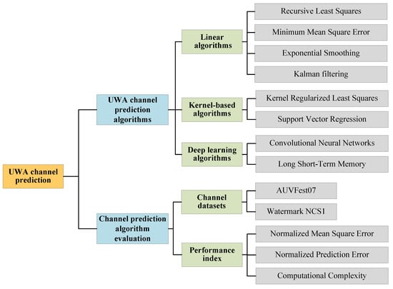
Figure 1. The main structure of this paper.

• We introduce the application of UWA channel prediction technology in UWA communication.
• This paper classifies current UWA channel prediction techniques and introduces its principles, implementation methods, and specific applications.
• Based on the at-sea experiment dataset from the 2007 Autonomous Underwater Vehicle Festival (AUVFest07) [24] and the UnderWater AcousTic channEl Replay benchMARK (Watermark) [25], we comprehensively compare the existing typical underwater acoustic channel prediction algorithms under a unified system framework, and objectively analyze the prediction performance and computational complexity of these algorithms.
• We analyze the advantages and limitations of different algorithms based on the experimental results. Additionally, we discuss the existing challenges and potential future development directions of UWA channel prediction.

The paper is organized as follows: In Section 2, we review and summarize the typical algorithms of UWA channel prediction and their application in communication systems. In Section 3, we describe a comparative experiment based on real data collected during experiments to test the prediction performance of typical algorithms. In Section 4, we provide concluding remarks.

Notation: Throughout the paper, the superscripts ^*, ^T, ^H, <> denote the conjugate, transpose, conjugate transpose, and ensemble average, respectively. Scalars are written in lower case, vectors are in lower case bold, and matrices are in bold capitals. All acronyms used in this paper are defined in Table 1.

Table 1. Acronyms used in this paper.

Acronym	Full Name	Acronym	Full Name
UWA	underwater acoustic	CS	compressed sensing
CSI	channel state information	SNR	signal-to-noise ratio
BER	bit error ratio	NMSE	normalized mean square error
CIR	channel impulse response	KAF	kernel adaptive filter
OFDM	orthogonal frequency-division multiplexing	KRLS	kernel recursive least squares
RLS	recursive least squares	SVM	support vector machine
MMSE	minimum mean square error	SVR	support vector regression
LMMSE	linear minimum mean square error	RNN	recurrent neural networks
ES	exponential smoothing	LSTM	long short-term memory

2. Algorithms for Underwater Acoustic Channel Prediction

Figure 2 shows the whole process of channel prediction. When the number of observed historical channels is small, linear algorithms can be used to predict; when the number is large enough, algorithms such as deep learning can be used for prediction.

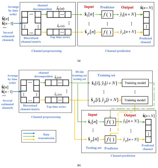
Figure 2. The process of channel prediction. (a) Algorithms that do not require training. (b) Algorithms that require training.

When explaining the channel prediction algorithms, the channel is uniformly defined as a coherent multipath channel in the time domain, and can be expressed as

$$h(\tau ,t)=\sum _{p=0}^{P-1}{h}_p\left(t\right)\delta (\tau -{\tau }_p\left(t\right)),$$

(1)

where P is the number of channel taps, t is the time when the channel is observed, and $\tau$ is the delay variable. $h_p\left(t\right)$ and ${\tau }_p\left(t\right)$ represent the p-th tap and the corresponding delay at time t, respectively.

Then, $h(\tau ,t)$ is discretized in time, and the channel at time n can be expressed as

$$\mathbf{h}\left[n\right]=[h_1\left(n\right)h_2\left(n\right)\dots h_P\left(n\right)]$$

(2)

We predict $\mathbf{h}\left[n\right]$. At time n, we choose to use the past M estimated channels $\left\{\tilde{\mathbf{h}}\left[n\right],\tilde{\mathbf{h}}[n-1],\dots ,\tilde{\mathbf{h}}[n-M+1]\right\}$ to obtain the predicted channel $\widehat{\mathbf{h}}[n+N]$ at n + N time, where

$$\begin{array}{cc}\hfill \tilde{\mathbf{h}}\left[n\right]=& [{\tilde{h}}_1\left(n\right){\tilde{h}}_2\left(n\right)\dots {\tilde{h}}_P\left(n\right)]\hfill \\ \hfill \widehat{\mathbf{h}}[n+N]=& [{\widehat{h}}_1(n+N){\widehat{h}}_2(n+N)\dots {\widehat{h}}_P(n+N)]\hfill \end{array}$$

(3)

In the actual prediction process, we predict each tap separately and then combine them into the predicted channel $\widehat{\mathbf{h}}[n+N]$. At this time, the prediction problem of the channels is transformed into a time series prediction problem about tap ${\tilde{h}}_P\left(n\right)$.

When we predict tap ${\tilde{h}}_P\left(n\right)$, the input of the predictor can be expressed as ${\tilde{\mathbf{x}}}_p\left[n\right]$, and the output of the predictor is expressed as ${\widehat{y}}_p[n+N]$; ${\widehat{y}}_p[n+N]$ is the predicted value of the p-th tap at $n+N$ time. The prediction process of the predictors can be expressed as

$${\widehat{y}}_p[n+N]=f\left({\tilde{\mathbf{x}}}_p\left[n\right]\right),$$

(4)

where

$$\begin{array}{cc}\hfill {\widehat{y}}_p[n+N]& ={\widehat{h}}_p(n+N)\hfill \end{array}$$

(5)

$$\hspace{1em}\hspace{1em}\hspace{1em}\hspace{1em}\hspace{1em}\hspace{1em}\hspace{1em}\hspace{1em}\hspace{1em}\hspace{1em}\hspace{1em} \begin{array}{cc}\hfill {\tilde{\mathbf{x}}}_p\left[n\right]& ={[{\tilde{h}}_p\left(n\right){\tilde{h}}_p(n-1)\dots {\tilde{h}}_p(n-M+1)]}^T\hfill \end{array}$$

(6)

When the predicted values of all taps at time $n+N$ are obtained, we can obtain the predicted channel $\widehat{\mathbf{h}}[n+N]$ according to Equation (3).

Figure 2 shows the whole process of channel prediction. When the number of observed historical channels is small, the linear algorithm can be used to predict; when the number is large enough, algorithms such as deep learning can be used for prediction. From Figure 2 and the above equations, it can be inferred that Equation (4) is crucial for channel prediction. In the following subsections, we will categorically investigate the prediction process ${\widehat{y}}_p[n+N]=f\left({\tilde{\mathbf{x}}}_p\left[n\right]\right)$ of the predictor.

In this paper, the variable definitions concerning channel prediction are presented in Table 2.

Table 2. The definitions of variables related to channel prediction.

Variable	Definition
P	Number of channel taps (number of predictors)
M	Number of historical channels for prediction
N	Predicting the channel after N steps
$N_{train}$	Number of training set channels
$N_{test}$	Number of testing set channels
$\tilde{\mathbf{h}}\left[n\right]$	Estimated channel at time n
$\widehat{\mathbf{h}}[n+N]$	Predicted channel at time n + N
$\tilde{\mathbf{h}}[n+N]$	Estimated channel at time n + N, which is used to calculate the channel prediction error
${\tilde{\mathbf{x}}}_p\left[n\right]$	Input of the predictor for the p-th tap
${\widehat{y}}_p[n+N]$	Output of the predictor for the p-th tap
${\tilde{y}}_p[n+N]$	Estimate value of the p-th tap at the time n + N, which is used to calculate the predictor error

2.1. Linear Algorithms

Linear predictions are the earliest and most widely used algorithms in UWA channel prediction. Typical algorithms include RLS, minimum mean square error (MMSE), exponential smoothing (ES), and Kalman filtering, where RLS and MMSE are methods used to determine the coefficients of linear regression algorithms.

In linear regression algorithms, historical channel data can be used to obtain the predicted channel through linear combination. Linear regression prediction algorithms can generally be expressed as

$${\widehat{y}}_p[n+N]={\mathbf{w}}^T{\tilde{\mathbf{x}}}_p\left[n\right],$$

(7)

where $\mathbf{w}$ represents the linear weighting coefficient.

RLS: RLS is a typical parameter determination method. As a recursive algorithm, RLS can re-estimate the weighting coefficients using the least square criterion based on the current input signal. The disadvantage of RLS is that, compared with other linear algorithms, the coefficient update process is more complicated and the amount of calculation required is larger.

The prediction process of the RLS algorithm is shown in Algorithm 1, where $\delta$ is a small constant, $\mathbf{u}\left[n\right]$ is the gain matrix, $\mathbf{T}\left[n\right]$ is the inverse matrix of the correlation matrix, $\mathbf{w}\left[n\right]$ is the prediction coefficients, $e\left[n\right]$ is the prediction error at time n, and $\lambda$ is the forgetting factor.

Algorithm 1 RLS prediction algorithm

Input: ${\tilde{\mathbf{x}}}_p\left[n\right]$ Output:  ${\widehat{y}}_p[n+N]$ Initialization: $\mathbf{w}\left[0\right]=0$, $\mathbf{T}\left[0\right]={\delta }^{-1}I$ for n = N, N + 1, … do    ${\displaystyle \mathbf{u}\left[n\right]=\frac{\mathbf{T}[n-N]{\tilde{\mathbf{x}}}_p[n-N]}{\lambda +{\tilde{\mathbf{x}}}_p^H[n-N]\mathbf{T}[n-N]{\tilde{\mathbf{x}}}_p[n-N]}}$    ${\widehat{y}}_p\left[n\right]={\mathbf{w}}^T[n-N]{\tilde{\mathbf{x}}}_p[n-N]$    $e\left[n\right]={\tilde{y}}_p\left[n\right]-{\widehat{y}}_p\left[n\right]$    $\mathbf{w}\left[n\right]=\mathbf{w}[n-N]+\mathbf{u}\left[n\right]e\left[n\right]$    $\mathbf{T}\left[n\right]={\lambda }^{-1}\mathbf{T}[n-N]-{\lambda }^{-1}\mathbf{u}\left[n\right]{\tilde{\mathbf{x}}}_p^H[n-N]\mathbf{T}[n-N]$ end for

Generally, in order to simplify the operation, the channel can be modeled as a sparse structure. Stojanovic et al. utilized the sparse multipath structure of the channel and employed the RLS algorithm for channel prediction [4]. In [4], the authors proposed a joint prediction based on all channel coefficients from each different receive element. Based on [4], Stojanovic et al. designed an adaptive OFDM system, and provided real-time adaptive modulation results in a sea experiment [26]. Ref. [27] validated the performance of the prediction algorithm proposed in [4], using experimental data from the South China Sea.

In UWA channel prediction, channel estimation methods also need to be considered. Under the condition of a sparse channel and using the RLS prediction method, compressed sensing (CS) can obtain a lower BER than MMSE channel estimation methods in an OFDM adaptive system [28].

In addition to adaptive modulation, ref. [29] used the channel predicted by RLS for precoding at the transmitter, resulting in energy savings for certain specific nodes in cooperative communications. Ref. [30] performed channel prediction in the delay-Doppler domain. The receiver predicted the channel for the next data block based on the estimated channel of the previous data block, and utilized the prediction values to perform channel equalization to improve system performance.

When the channel observation data have a long-time span, the periodic change of the channel can be used to predict. Sun and Wang modeled the channel as a combination of a Markov process and an environment variable. To improve the prediction performance, data from the same time period but one epoch prior were taken into consideration. When the time span of the experimental data was 250 h, channel prediction achieved good performance [31].

MMSE: In the MMSE algorithm, all known channels need to be used to calculate the covariance matrix and to perform the matrix inversion. Furthermore, the data are required to be generalized stationary. In practical applications, as the amount of data increases, the covariance matrix can be updated. The determination method of the coefficient is as follows:

The prediction process of the MMSE algorithm is shown in Algorithm 2, where ${\mathbf{C}}_{\mathbf{xx}}$ is the variance of ${\tilde{\mathbf{x}}}_p\left[n\right]$, ${\mathbf{c}}_{\mathbf{xy}}$ is the covariance of ${\tilde{\mathbf{x}}}_p\left[n\right]$ and ${\tilde{y}}_p\left[n\right]$, $\mathbf{w}$ is the weight coefficient, and ${\mathit{\mu }}_{\mathbf{x}}$ and ${\mu }_{\mathbf{y}}$ are the mean values of variables ${\tilde{\mathbf{x}}}_p\left[n\right]$ and ${\tilde{y}}_p\left[n\right]$, respectively.

Algorithm 2 MMSE prediction algorithm

Input: ${\tilde{\mathbf{x}}}_p\left[n\right]$ Output:  ${\widehat{y}}_p[n+N]$ for n = 1, 2, … do    ${\mathbf{C}}_{\mathbf{xx}}=E\left\{[{\tilde{\mathbf{x}}}_p-{\mathit{\mu }}_{\mathbf{x}}]{[{\tilde{\mathbf{x}}}_p-{\mathit{\mu }}_{\mathbf{x}}]}^T\right\}$    ${\mathbf{c}}_{\mathbf{xy}}=E\left\{[{\tilde{\mathbf{x}}}_p-{\mathit{\mu }}_{\mathbf{x}}]{[{\tilde{y}}_p-{\mu }_{\mathbf{y}}]}^T\right\}$    $\mathbf{w}={\mathbf{C}}_{\mathbf{xx}}^{-1}{\mathbf{c}}_{\mathbf{xy}}$    ${\widehat{y}}_p[n+N]={\mathbf{w}}^T{\tilde{\mathbf{x}}}_p\left[n\right]$ end for

Stojanovic et al. applied channel prediction to single input multiple output (SIMO) OFDM systems [32]. In order to expand the system throughput, pilots were not installed in all OFDM data blocks but rather were placed at regular intervals. At the receiver, the channels estimated by pilots were exploited to predict the channel for OFDM data blocks without pilot symbols based on the MMSE criterion. Additionally, the system can also predict the channel for the next transmission time, providing information for the power allocation algorithm proposed in the literature.

In [33], the authors proposed a sparse channel parameter feedback method based on CS theory in adaptive modulation OFDM systems. Subsequently, the predicted channels were transformed into the frequency domain, where the received signal-to-noise ratio (SNR) for each subcarrier could be obtained, and the appropriate modulation scheme could be selected. The experimental results showed that, compared with the fixed modulation scheme, adaptive modulation based on CS channel estimation and linear minimum mean square error (LMMSE) channel prediction achieved better performance.

ES: ES is a typical algorithm used in the field of time series analysis, which was first proposed by Robert [34]. In the ES algorithm, the predicted value is represented as the exponential weighted sum of historical channel data. It uses a smoothing factor that assigns higher weights to data points that are closer to the predicted value. Three basic variations of ES are commonly used for channel prediction: simple ES, trend-corrected ES, and the Holt–Winters’ method.

The prediction process of the simple ES algorithm is shown in Algorithm 3. For the ES algorithm, M and N in Equations (5) and (6) are set to 1; a is the pre-defined parameter.

Algorithm 3 ES prediction algorithm

Input: ${\tilde{x}}_p\left[n\right]={\tilde{h}}_p\left(n\right)$ Output:  ${\widehat{y}}_p[n+1]={\widehat{h}}_p(n+1)$ Initialization:  ${\widehat{y}}_p\left[1\right]=0$ for n = 1, 2, 3, … do       ${\widehat{y}}_p[n+1]=a{\tilde{x}}_p\left[n\right]+(1-a){\widehat{y}}_p\left[n\right]$ end for

The Holt–Winters algorithm was employed by Wang et al. to predict the SNR of the channel, which was then used for adaptive scheduling of point-to-point data transmission [35]. The algorithm also focused on seasonal prediction models on large time scales. By predicting the channel SNR, the system can adaptively determine the time slot of data transmission, resulting in improved energy efficiency compared to fixed-time transmission.

In [36], the Holt–Winters algorithm was also employed to predict the SNR for replacing the outdated information. The predicted information was then utilized for data transmission between underwater target users and the surface central node. The SNR data used in the simulation range from 1 to 100 h. The results show that the system using the prediction algorithm would perform better than that using the feedback data by calculating the normalized mean square error (NMSE).

Kalman filtering: As a time-domain filtering method, a Kalman filter can recursively obtain the estimator by using the observations related to the state equation. In UWA communication, it is widely used in channel estimation [37], channel equalization [38], channel tracking [39,40,41], and multi-user detection [42].

In [43], by exploiting channel knowledge obtained from prediction techniques, the author proposed an OFDM scheme which can adaptively adjust the length of the cyclic prefix. Channel prediction was operated in the frequency domain, and the evolution of a single sub-channel was tracked via a Kalman filter. The experiments demonstrated that the proposed approach reduced the BER of communication and avoided exchange of overhead information between the transmitting and receiving nodes.

2.2. Kernel-Based Algorithms

Linear algorithms have advantages in terms of simplicity and real-time performance, but have limitations when dealing with channel prediction. Linear algorithms have a simple structure and are easily modeled. Generally, they do not require historical channel data for training and can perform online prediction directly. However, the lack of data-fitting ability makes it difficult to deal with nonlinear problems. In such cases, the use of more complex kernel-based algorithms is a more appropriate choice. In general, kernel-based algorithms are commonly performed using kernel methods, which can map data to high-dimensional space through a kernel trick. By utilizing linear calculations in the high-dimensional space, it becomes possible to achieve non-linear fitting of the channel data [44]. Typical kernel-based algorithms include the kernel adaptive filter (KAF) and support vector machine (SVM) [45]. Both algorithms can achieve accurate fitting of complex data patterns.

KAF: KAF can be considered as an extension of linear filtering algorithms in the kernel space. Typical KAF algorithms include the kernel least mean squares algorithm [46], the kernel recursive least squares (KRLS) algorithm [47], and the kernel affine projection algorithm [48]. Based on these three typical algorithms, a number of improved algorithms have been introduced. A comparison of typical KAF algorithms was provided in [49].

Taking KRLS as an example, it can be viewed as an extension of RLS in a high-dimensional feature space. The prediction process of the KRLS algorithm is shown in Algorithm 4, where $\mathbf{U}\left[n\right]$ is the kernel inverse matrix, $\mathbf{d}\left[n\right]$ is the characteristic space coefficient matrix, $\mathbf{q}\left[n\right]$ and $r\left[n\right]$ are adaptive control quantities, $e\left[n\right]$ is the prediction error, $\kappa \left(\right)$ is the kernel function, and $\gamma$ is the regularization factor.

Algorithm 4 KRLS prediction algorithm

Input: ${\tilde{\mathbf{x}}}_p\left[n\right]$ Output:  ${\widehat{y}}_p[n+N]$ Initialization: $\mathbf{U}\left[0\right]={(\kappa ({\tilde{\mathbf{x}}}_p\left[0\right],{\tilde{\mathbf{x}}}_p\left[0\right])+\gamma )}^{-1}$, $\mathbf{d}\left[0\right]=\mathbf{U}\left[0\right]{\tilde{y}}_p\left[N\right]$ for n = N, N + 1, N + 2, … do       $\mathbf{P}\left[n\right]={[\kappa ({\tilde{\mathbf{x}}}_p[n-N],{\tilde{\mathbf{x}}}_p\left[0\right]),\dots ,\kappa ({\tilde{\mathbf{x}}}_p[n-N],{\tilde{\mathbf{x}}}_p[n-N-1])]}^T$       ${\widehat{y}}_p\left[n\right]=\mathbf{P}{\left[n\right]}^T\mathbf{d}[n-N]$       $e\left[n\right]={\tilde{y}}_p\left[n\right]-{\widehat{y}}_p\left[n\right]$       $\mathbf{q}\left[n\right]=\mathbf{U}[n-N]\mathbf{P}\left[n\right]$       $r\left[n\right]=\gamma +\kappa ({\tilde{\mathbf{x}}}_p[n-N],{\tilde{\mathbf{x}}}_p[n-N])-\mathbf{q}{\left[n\right]}^T\mathbf{P}\left[n\right]$       $\mathbf{U}\left[n\right]=r{\left[n\right]}^{-1}\left[\begin{array}{cc}\mathbf{U}[n-N]r\left[n\right]+\mathbf{q}\left[n\right]\mathbf{q}{\left[n\right]}^T& -\mathbf{q}\left[n\right]\\ -\mathbf{q}{\left[n\right]}^T& 1\end{array}\right]$       $\mathbf{d}\left[n\right]=\left[\begin{array}{c}\mathbf{d}[n-N]-\mathbf{q}\left[n\right]r{\left[n\right]}^{-1}e\left[n\right]\\ r{\left[n\right]}^{-1}e\left[n\right]\end{array}\right]$ end for

From the formulas, it can be observed that in the KRLS algorithm, the dimension of $\mathbf{U}\left[n\right]$ is related to the number of samples. To address this issue, several improvement algorithms have been proposed, such as sliding window KRLS [50] and fixed-budget KRLS [51].

KAF has found extensive application in wireless channel prediction and time series analysis. However, the ordinary KAF algorithm cannot deal with the interference of impulse noise. In order to enhance the robustness of traditional KAF methods, such as KRLS, we can choose to control the dictionary energy [52]. Refs. [53,54] improved the prediction performance of nonlinear time series by using a generalized tanh function and an energy dynamic threshold, respectively. Ref. [55] proposed using a sparse sliding-window KRLS to achieve dynamic dictionary sample updates, which outperformed an approximate linear dependency KRLS in fast time-varying multiple-input multiple-output systems.

In 2021, Liu et al. designed a comparative experiment to assess the performance of prediction algorithms in addressing the subcarrier resource allocation problem in downlink OFDM systems. They compared the proposed CsiPreNet model with KRLS, RLS, and several neural networks [56]. Then, in 2023, Liu et al. proposed a system that incorporated a per-subcarrier channel temporal correlation for channel optimization and subsequent channel feedback [57]. In the evaluation, the approximate linear dependency KRLS and other algorithms were also compared. The results of both experiments revealed that the approximate linear dependency KRLS performed better than linear algorithms and traditional neural networks.

SVM and SVR: SVM is developed by Vapnik [58], and is mainly applied in classification problems, while support vector regression (SVR) is more suitable for function fitting. SVM has been applied in the underwater acoustics field, but has mainly focused on underwater target classification, channel equalization, and so on [59,60]. In terms of time series prediction, it is extensively reported in [61].

Taking SVR as an example. Given a training set $\left\{{\tilde{\mathbf{x}}}_p\left[i\right],{\tilde{y}}_p[i+N]\right\},i=1,2,3,\dots N_{train}$, the input–output relationship of the predictor during training is as follows:

$$\begin{array}{c}\hfill {\tilde{y}}_p[i+N]=f_{SVR}\left({\tilde{\mathbf{x}}}_p\left[i\right]\right)={\mathbf{w}}^{\mathbf{T}}\phi \left({\tilde{\mathbf{x}}}_p\left[i\right]\right)+b,\end{array}$$

(8)

where $\phi$ is a high-dimensional mapping function, $\mathbf{w}$ is a weight vector, and b is the bias term. The optimization goal during training can be expressed as

$$\begin{array}{c}\hfill \underset{\mathbf{w},b}{min}\frac{1}{2}{∥\mathbf{w}∥}^2+C\sum _{i=1}^{N_{train}}({\gamma }_i+{\gamma }_i^{*})\end{array}$$

(9)

$$\begin{array}{c}\hfill s.t.\left\{\begin{array}{c}{\tilde{y}}_p[i+N]-{\mathbf{w}}^T{\tilde{\mathbf{x}}}_p\left[i\right]-b\le \theta +{\gamma }_i^{*}\\ {\mathbf{w}}^T{\tilde{\mathbf{x}}}_p\left[i\right]+b-{\tilde{y}}_p[i+N]\le \theta +{\gamma }_i\end{array}\right.\\ \hfill i=1,2,\dots N_{train},\end{array}$$

(10)

where $\theta$ is the margin of tolerance, C is the regularization constant, and ${\gamma }_i^{*}$ and ${\gamma }_i$ are slack variables. To resolve this convex optimization problem, the Lagrangian multipliers $\beta ,{\beta }^{*}$ are introduced, and the corresponding dual optimization problem of Equation (9) can be expressed as

$$\begin{array}{cc}\hfill \underset{\beta ,{\beta }^{*}}{max}\mathbf{w}(\beta ,{\beta }^{*})& =-\theta \sum _{i=1}^{N_{train}}({\beta }_i+{\beta }_i^{*})+\sum _{i=1}^{N_{train}}{\tilde{y}}_p[i+N]({\beta }_i^{*}-{\beta }_i)\hfill \end{array}$$

$$\begin{array}{cc}\hfill -\frac{1}{2}& \sum _{i,j}^{N_{train}}({\beta }_i^{*}-{\beta }_i)({\beta }_j^{*}-{\beta }_j)\kappa ({\tilde{\mathbf{x}}}_p\left[i\right],{\tilde{\mathbf{x}}}_p\left[j\right])\hfill \end{array}$$

(11)

$$\begin{array}{cc}\hfill & s.t.\sum _{i=1}^{N_{train}}{\beta }_i^{*}=\sum _{i=1}^{N_{train}}{\beta }_i\hfill \\ \hfill & 0\le {\beta }_i,{\beta }_i^{*}\le Ci=1,\dots ,N_{train}\hfill \end{array}$$

(12)

When the training is over, the optimal $\beta ,{\beta }^{*}$ can be obtained and the optimal fitted regression equation for prediction can be expressed as

$$\begin{array}{c}\hfill {\widehat{y}}_p[n+N]=f_{SVR}\left({\tilde{\mathbf{x}}}_p\left[n\right]\right)=\sum _{i=1}^{N_{train}}({\beta }_i^{*}-{\beta }_i)\kappa ({\tilde{\mathbf{x}}}_p\left[i\right],{\tilde{\mathbf{x}}}_p\left[n\right])\end{array}$$

(13)

The prediction process of the SVR algorithm is shown in Algorithm 5.

Algorithm 5 SVR prediction algorithm

Input: training set $\left\{{\tilde{\mathbf{x}}}_p\left[i\right],{\tilde{y}}_p[i+N]\right\},i=1,2,3,\dots N_{train}$ testing set $\left\{{\tilde{\mathbf{x}}}_p\left[n\right],{\tilde{y}}_p[n+N]\right\},n=1,2,3,\dots N_{test}$ Output:  ${\widehat{y}}_p[n+N]$ training process: Set the values of b, $\theta$, C, and use the training set to obtain the best $\beta ,{\beta }^{*}$. predicting process:  for n = 1, 2, 3, … $N_{test}$ do        ${\widehat{y}}_p[n+N]=f_{SVR}\left({\tilde{\mathbf{x}}}_p\left[n\right]\right)$  end for

In underwater acoustic channel prediction and adaptive modulation, SVM and SVR serve different purposes. The SVM algorithm is commonly used for classification tasks. In adaptive modulation systems, it is often employed to directly determine the optimal modulation scheme based on historical channel data. On the other hand, the SVR algorithm is more suitable for regression tasks. It can fit the historical channel data and predict the channel at the next time step, and then the adaptive system can adapt to the channel characteristics effectively.

In [62], the authors applied adaptive modulation to long distance UWA communication, utilizing the SVM and SVR algorithms. Since the channel in long-distance UWA communication changes more rapidly than that in general UWA communication, the direct use of a feedback channel will impose significant limitations on the communication performance. The authors proposed adding an abstraction layer, in which abstract features were extracted by SVM or SVR, and the modulation mode was selected after channel classification or performance prediction, which can improve the adaptability of the system to mismatched channels. The experimental results demonstrated that the prediction algorithm based on SVR achieved higher throughput in practice.

2.3. Deep Learning Algorithms

Deep neural networks perform channel prediction by using nonlinear layers to construct complex networks [63]. Deep learning algorithms possess remarkable fitting capabilities for data and have found widespread application in fields such as image classification and language translation. Algorithms such as convolutional neural networks (CNNs) and recurrent neural networks (RNNs) are utilized for time series prediction [64,65,66]. In the field of communication, algorithms represented by CNNs and a variant of RNN, long short-term memory (LSTM), are also applied to channel prediction [67,68,69]. LSTM has already been applied in time series processing, while CNN is commonly used for image classification [70]. To utilize CNN for time series and channel prediction, it is common to employ a one-dimensional CNN model instead of the commonly used two-dimensional model for image classification.

CNN: Taking a one-dimensional CNN model as an example, it includes input, 1D convolution, 1D pooling and flattening layers. The convolution layer can analyze characteristics of the input data through convolution operations. It uses a filter to scan the input data matrix and generate the corresponding feature map. We use a filter to describe the convolutional layer, where the weight of the filter is defined as ${\mathbf{W}}_{con}$, the data input to the convolutional layer is ${\tilde{\mathbf{x}}}_p\left[n\right]$, the activation function is defined as $f_{con}\left(\right)$, and the bias parameter is defined as b. Then, the output ${\mathbf{C}}^{*}$ of the convolutional layer can be written as:

$${\mathbf{C}}^{*}=f_{con}({\tilde{\mathbf{x}}}_{\mathbf{p}}\left[\mathbf{n}\right]\otimes {\mathbf{W}}_{\mathbf{con}}+b)$$

(14)

The convolutional result ${\mathbf{C}}^{*}$ will enter the pooling layer, which can reduce the size of the feature map and extract more abstract features. Taking the maximum pooling layer as an example, its output $C^{*}$ can be expressed as

$$C^{*}=\max \left({\mathbf{C}}^{*}\right)$$

(15)

Assuming that the number of filters is $N_{con}$, the feature map passing through the pooling layer can be expressed as $[C_1^{*},C_2^{*},\dots ,C_{N_{con}}^{*}]$.

Finally, the fully connected (FC) layer combines the elements of the feature map and maps them to the label space of the sample, it can be expressed as

$${\widehat{y}}_p[n+N]=f_{FC}(C_1^{*},C_2^{*},\dots ,C_{N_{con}}^{*}).$$

(16)

The whole prediction process of the one-dimensional CNN can be simplified as

$${\widehat{y}}_p[n+N]=f_{CNN}\left({\tilde{\mathbf{x}}}_p\left[n\right]\right).$$

(17)

The prediction process of the CNN algorithm is shown in Algorithm 6.

Algorithm 6 CNN prediction algorithm

Input: training set $\left\{{\tilde{\mathbf{x}}}_p\left[i\right],{\tilde{y}}_p[i+N]\right\},i=1,2,3,\dots N_{train}$ testing set $\left\{{\tilde{\mathbf{x}}}_p\left[n\right],{\tilde{y}}_p[n+N]\right\},n=1,2,3,\dots N_{test}$ Output:  ${\widehat{y}}_p[n+N]$ training process: Set the values of $N_{con}$, convolution kernel size, batch size, epoch, learning rate, loss function. Use the training set to obtain the best model. predicting process: for n = 1, 2, 3, … $N_{test}$ do       ${\widehat{y}}_p[n+N]=f_{CNN}\left({\tilde{\mathbf{x}}}_p\left[n\right]\right)$ end for

LSTM: LSTM is a special RNN model that avoids long-term dependency problems and is well-suited for time series prediction. A typical structure of an LSTM cell is shown in Figure 3. The data update process of each part is as follows:

$$\begin{array}{c}\hfill \mathbf{Input}\mathbf{Gate}\\ \hfill {\mathbf{\Phi }}_n^i& =\sigma ({\mathbf{W}}^i·[{\mathbf{k}}_{n-1},{\mathbf{x}}_n]+{\mathbf{b}}^i)\hfill \end{array}$$

(18)

$$\begin{array}{c}\hfill \mathbf{Forget}\mathbf{Gate}\\ \hfill {\mathbf{\Phi }}_n^f& =\sigma ({\mathbf{W}}^f·[{\mathbf{k}}_{n-1},{\mathbf{x}}_n]+{\mathbf{b}}^f)\hfill \end{array}$$

(19)

$$\begin{array}{c}\hfill \mathbf{Output}\mathbf{Gate}\\ \hfill {\mathbf{\Phi }}_n^o& =\sigma ({\mathbf{W}}^o·[{\mathbf{k}}_{n-1},{\mathbf{x}}_n]+{\mathbf{b}}^o)\hfill \end{array}$$

(20)

$$\begin{array}{cc}\hfill {\mathbf{k}}_n& ={\mathbf{\Phi }}_n^o\ast \tanh \left({\mathbf{v}}_n\right)\hfill \end{array}$$

(21)

$$\begin{array}{cc}\hfill \hspace{1em}\hspace{1em}\hspace{1em}\hspace{1em}\hspace{1em}\hspace{1em}\hspace{1em}\hspace{1em}\hspace{1em}\mathbf{Cell}\mathbf{State}& \hfill \\ \hfill \hspace{1em}\hspace{1em}\hspace{1em}\hspace{1em}\hspace{1em}\hspace{1em}\hspace{1em}\hspace{1em}\hspace{1em}{\mathbf{v}}_n& ={\mathbf{\Phi }}_n^f\ast {\mathbf{v}}_{n-1}+{\mathbf{\Phi }}_n^i\ast \tanh ({\mathbf{W}}_c·[{\mathbf{k}}_{n-1},{\mathbf{x}}_n]+{\mathbf{b}}_f)\hfill \end{array}$$

(22)

where ${\mathbf{W}}^i,{\mathbf{W}}^c,{\mathbf{W}}^f$ and ${\mathbf{W}}^o$ are the coefficient weight matrices, and ${\mathbf{b}}^i,{\mathbf{b}}^c,{\mathbf{b}}^f$ and ${\mathbf{b}}^o$ are the bias vectors. ${\mathbf{\Phi }}_n^i,{\mathbf{\Phi }}_n^f$ and ${\mathbf{\Phi }}_n^o$ are the input gate, forget gate, and the output gate, respectively. ${\mathbf{k}}_n$ is the hidden state, ${\mathbf{v}}_n$ is the unit state, and ${\mathbf{x}}_n$ is the unit input. $\sigma \left(\right)$ is the sigmoid function. For LSTM channel prediction, Equation (4) can be rewritten as

$${\widehat{y}}_p[n+N]=f_{LSTM}\left({\tilde{\mathbf{x}}}_p\left[n\right]\right).$$

(23)

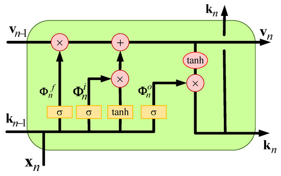
Figure 3. Typical structure of LSTM cell.

The prediction process of the LSTM algorithm is shown in Algorithm 7.

Algorithm 7 LSTM prediction algorithm

Input: training set $\left\{{\tilde{\mathbf{x}}}_p\left[i\right],{\tilde{y}}_p[i+N]\right\},i=1,2,3,\dots N_{train}$ testing set $\left\{{\tilde{\mathbf{x}}}_p\left[n\right],{\tilde{y}}_p[n+N]\right\},n=1,2,3,\dots N_{test}$ Output:  ${\widehat{y}}_p[n+N]$ training process: Set the number of hidden layers, the number of hidden layer units, batch size, epoch, learning rate, loss function. Use the training set to obtain the best model. predicting process: for n = 1, 2, 3, … $N_{test}$ do       ${\widehat{y}}_p[n+N]=f_{LSTM}\left({\tilde{\mathbf{x}}}_p\left[n\right]\right)$ end for

In [71], a one-dimensional CNN was employed for predicting the performance of UWA communications based on CIR. Two datasets were used in the experiments, and the results demonstrated that the predictive performance of the CNN was superior to traditional machine learning methods on any of the datasets. Furthermore, when the two datasets were combined into a single dataset, the model still exhibited favorable performance.

In [56], a learning model named CsiPreNet was designed by Liu et al., which was represented as a combination of CNN and LSTM. The CsiPreNet employed CNN to extract the channel frequency domain features and then utilizeed LSTM to capture the temporal correlations and to make predictions. In the simulation, the author compared and analyzed the proposed CsiPreNet with LSTM, a back propagation neural network, and RLS algorithms. The results revealed that the CsiPreNet algorithm achieved the best performance under both error calculation methods.

In [72], the authors employed LSTM for channel prediction and then utilized reinforcement learning to improve the adaptive modulation system using predicted channels. The results showed that the LSTM method can improve network throughput under the constraint of BER. In order to improve the performance of LSTM, traditional LSTM can also be combined with other models, such as a self-attention mechanism [73].

3. Experimental Evaluation

In current papers on underwater acoustic channel prediction, the performance of algorithms is usually verified by comparative experiments. However, these experiments suffer from certain shortcomings. Firstly, only a few typical algorithms are involved. Secondly, different datasets are used between different experiments, making it difficult to achieve a comprehensive understanding and comparison of algorithm performance. In order to achieve a more effective comparison of prediction algorithms, in this section, we will first select typical algorithms that have been widely verified in the previous literature, then employ the same dataset for comparison, and, finally, utilize the same evaluating indicator to quantify the performance differences among the algorithms. The above methods can provide a more reliable and comprehensive understanding, which is helpful to evaluate the effectiveness and applicability of various prediction algorithms.

3.1. Dataset Description

In the performance comparison experiments of different algorithms, CIRs were obtained from the AUVFest07 experiment [24,40,41,74] and the Watermark database [25,75]. Figure 4 and Figure 5 illustrate the equipment deployment and CIR obtained in AUVFest07 calm sea conditions, AUVFest07 rough sea conditions, and Watermark NCS1, respectively. In Figure 5, the ordinate represents the observed time of the channel, and the abscissa represents the delay spread of the channel.

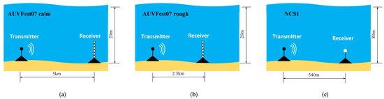
Figure 4. Sketch of equipment deployment. (a) AUVFest07 calm sea conditions, (b) AUVFest07 rough sea conditions, and (c) Watermark NCS1.

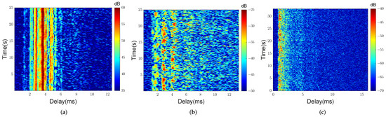
Figure 5. CIRs of (a) AUVFest07 calm sea conditions, (b) AUVFest07 rough sea conditions, and (c) Watermark NCS1 [41,75].

The AUVFest07 experiment was carried out in nearshore waters at a depth of 20 m. The sea conditions were relatively calm and rough, respectively. The experimental communication distances were 5 km and 2.3 km, respectively. The AUVFest07 experiment used 511 chips m-sequence signal, with frequency ranging from 15 kHz to 19 kHz. The duration of each packet was 25 s, which contained a total of 198 m-sequences. The channel delay was 5 ms and 12.5 ms, respectively, and the time interval of the channel at different times was ∼0.12 s.

In the Watermark database, we used the channel obtained from the Norwegian continental shelf (NCS1). The depth of the sea was 80 m, and the communication distance was 540 m. The equipment was fixed at the seabed, so the influence of equipment movement can be ignored.The signal type was pseudonoise, and its frequency ranged from 10 kHz to 18 kHz. One data packet contained more than 32.6 s of CIR. A total of 60 channel packets were obtained in ∼33 min. The channel delay was 32 ms, and the time interval of the channel was ∼0.032 s.

It can be observed from Figure 5 that the energy of the channel is carried by several main taps in AUVFest07 calm sea conditions, and the delays of the taps are relatively stable. In AUVFest07 rough sea conditions, the distribution of energy is more dispersed, and the delays of the main taps are not fixed. In the watermark NCS1, the initial taps have most of the energy of the channel.

In order to exhibit the different time-varying properties of the channels, we provide channel temporal coherence functions of three databases in Figure 6. One defines the channel temporal coherence function $\rho$ as [76].

$$\begin{array}{c}\hfill \rho (\Delta t)=\frac{⟨h^{*}(\tau ,t)h(\tau ,t+\Delta t)⟩}{\sqrt{⟨h^{*}(\tau ,t)h(\tau ,t)⟩⟨h^{*}(\tau ,t+\Delta t)h(\tau ,t+\Delta t)⟩}},\end{array}$$

(24)

where $\Delta t$ is the lag time. The channel temporal coherence reflects the speed of channel change to a certain extent. In Figure 6, it can be further reflected that, compared with AUVFest07 calm sea conditions, the channel has higher time variability in AUVFest07 rough sea conditions and Watermark NCS1, which are more challenging for prediction algorithms.

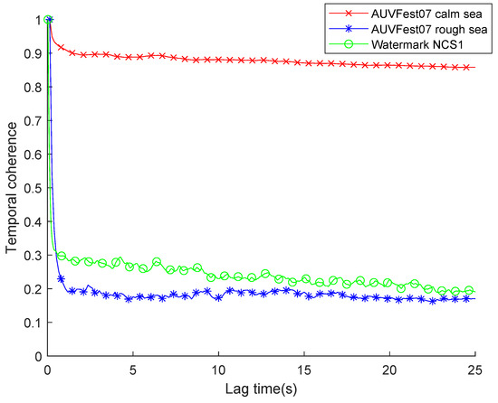
Figure 6. Channel temporal coherence as a function of lag time in AUVFest07 calm sea conditions, AUVFest07 rough sea conditions, and Watermark NCS1.

3.2. Experimental Process

Equation (1) defines the channel model, but in the actual prediction, our prediction object is the discrete channel $\mathbf{h}\left[n\right]$ in Equation (2), where the parameter P represents the number of taps that need to be predicted; how to determine its value is a key factor in prediction. In some studies, it is assumed that the channel has a sparse structure [26]. At this time, P has a small value, and the specific value is determined by the results of the channel estimation algorithms, such as CS [77,78] and sparse Bayesian learning [79]. Although this assumption holds reasonably well in Figure 5a, it fails in Figure 5b,c, because their channels are not quasi-static. Therefore, in this paper, we set the number of taps P as the number of sampling points of the channel, so that we can adapt to different channel structures. In AUVFest07 calm, AUVFest07 rough, and NCS1, the channel is uniformly sampled in the delay spread, and the values of P are 133, 125, and 510, respectively. As shown in Figure 5, the three public datasets directly provide a discrete channel matrix, so we can directly perform the channel preprocessing process in Figure 2, and then perform channel prediction.

Table 3 lists the algorithms for the channel prediction performance simulation. We set the parameter M to 4 and N to 1. The whole channel prediction process is shown in Figure 2, and the application of various algorithms is described in detail in Section 2. Different from linear and kernel-based algorithms, LSTM often requires a significant amount of historical channel samples for training and model optimization. In three channels, the number of training set channels $N_{train}$ is 20,560, 19,600, and 5940, and the number of testing sets $N_{test}$ is 50. In AUVFest07 calm and rough sea conditions, the channels estimated by the shift cyclic m-sequences are used to obtain sufficient training samples. In Watermark NCS1, multiple cycles of channels are used to train the LSTM algorithm. All the algorithms use the last 50 channel samples to verify the channel prediction performance.

Table 3. The algorithms for channel prediction performance simulation.

Algorithm	Algorithm Classification	Whether the Algorithm Needs Historical Channel Data to Train
RLS [4]	Linear Algorithm	No
LMMSE [33]	Linear Algorithm	No
ES [36]	Linear Algorithm	No
Kalman filtering [43]	Linear Algorithm	No
KRLS [56]	Kernel-Based Algorithm	No
SVR [62]	Kernel-Based Algorithm	Yes
LSTM [73]	Deep Learning Algorithm	Yes

This experiment needs to predict the complex value of the channel. Early studies found that for the complex value of the channel, predicting the real/imaginary can achieve better performance than predicting the amplitude/phase, because there is no phase mutation problem [80]. Therefore, the complex value of the channel obtained from the experiment is predicted separately by the real part and the imaginary part. The processing of the channel complex value is illustrated in Figure 7.

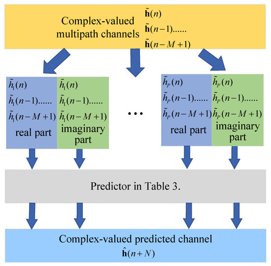
Figure 7. Processing of complex-valued channels.

Each tap of the channel is predicted separately and then combined together for error calculation and performance analysis. The NMSE and normalized channel prediction error are taken as the performance metrics. The NMSE is defined as

$$\begin{array}{c}\hfill NMSE=\frac{{\sum }_{n=1}^{N_{test}}{\left|\tilde{\mathbf{h}}[n+N]-\widehat{\mathbf{h}}[n+N]\right|}^2}{{\sum }_{n=1}^{N_{test}}{\left|\tilde{\mathbf{h}}[n+N]\right|}^2}.\end{array}$$

(25)

The normalized channel prediction error is defined as

$$\begin{array}{c}\hfill e_{nor}\left[n\right]=\frac{\sqrt{{\left|\tilde{\mathbf{h}}[n+N]-\widehat{\mathbf{h}}[n+N]\right|}^2}}{\sqrt{{\left|\tilde{\mathbf{h}}[n+N]\right|}^2}},\end{array}$$

(26)

where all variables have the same meanings as Table 2.

4. Experimental Results and Analysis

In the comparison experiment of the algorithms, we also consider the use of outdated channels as an algorithm to participate in the comparison. In the worst case, the system cannot perform channel prediction and can only rely on the outdated channel at the previous moment. The channel time-varying caused by the complex marine environment makes the actual channel and the outdated channel different, resulting in outdated channel errors. Our ultimate goal is to eliminate this error through channel prediction. Therefore, by comparing the outdated channel error with the prediction error of each prediction algorithm, the performance of the channel prediction algorithm can be better reflected.

Table 4 and Figure 8 illustrate the errors defined by Equations (25) and (26), respectively. Note from Figure 8 that the prediction errors of the linear algorithms are generally higher than those of the kernel-based algorithms. Additionally, the deep learning algorithm performs better than all the other algorithms in AUVFest07 rough sea conditions and Watermark NCS1, but it does not perform well in AUVFest07 calm sea conditions.

Table 4. The NMSE of each algorithm in three channel databases.

Algorithm	AUVFest07 Calm	AUVFest07 Rough	NCS1
Outdated data	0.0995	0.8952	0.4097
RLS	0.0792	0.7190	0.3700
LMMSE	0.0754	0.6312	0.3352
ES	0.0826	0.7992	0.4080
Kalman filtering	0.0811	0.6697	0.3363
KRLS	0.0784	0.6593	0.3496
SVR	0.2640	0.6276	0.3147
LSTM	0.2125	0.6128	0.3054

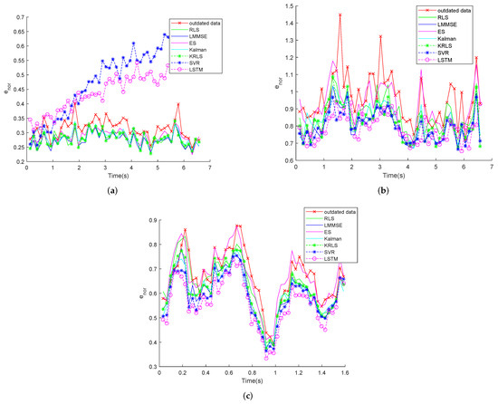
Figure 8. The normalized channel prediction errors defined by Equation (26) for different algorithms. (a) AUVFest07 calm sea. (b) AUVFest07 rough sea. (c) Watermark NCS1.

In theory, the data-fitting ability of the deep learning and kernel-based algorithms is better than that of linear algorithms. But in calm sea conditions, the performance of LSTM and SVR is not ideal—both of them need to be trained using historical channel data. Through research, we discover that the error mainly occurs on several main taps, which have strong energy. So, we study the real and imaginary parts of the tap carrying the maximum energy. In Figure 9, we provide the actual value over a time period of channel observation, as well as the predicted values of the KRLS, SVR, and LSTM algorithms to explore the reasons for the excessive error.

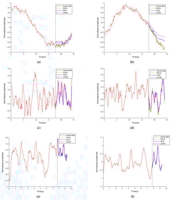
Figure 9. The actual values and predicted values of the maximum tap of the channel energy in AUVFest07 calm sea conditions, AUVFest07 rough sea conditions, and Watermark NCS1. (a) Calm real part. (b) Calm imaginary part. (c) Rough real part. (d) Rough imaginary part. (e) NCS1 real part. (f) NCS1 imaginary part.

In AUVFest07 calm sea conditions, the channel observation time is 25 s, of which the first 18 s channels are used as the training set. In theory, the training set should contain the complete change trend of the data, so that it can be extracted by the algorithms. However, in Figure 9a,b, we can observe that the real and imaginary parts fluctuate slowly, and the observation time of the channel samples is insufficient, resulting in the training set not containing the complete trend of channel data variations, which leads to a decline in the prediction performance. We note that this is particularly evident in the prediction of the imaginary part, where it is difficult for the predicted value to be less than the minimum value of the training set. Therefore, the lack of completeness of the training set is the key reason for the decline in prediction performance.

To further support the above conclusion, the trends of the real and imaginary parts of the tap carrying the maximum energy in AUVFest07 rough sea conditions and Watermark NCS1 are also presented in Figure 9c–f. It can be seen that at the same observation time, the channels of AUVFest07 rough and Watermark NCS1 change faster than those of AUVFest07 calm, so that the prediction algorithms can learn the complete change trend of the channel. At this point, the advantages of algorithms such as deep learning can be found, and their performance is demonstrated in Table 4. Therefore, it can still be considered that LSTM has the best performance in channel prediction.

Table 5 lists the computational complexity of the algorithms. M is the predictor order, D is the size of the KRLS dictionary, and $N_{train}$ is the number of SVR training samples. The computing complexity of the LSTM layer is $O(4n_{li}\times n_{lh}+4n_{lh}^2+3n_{lh}+n_{lh}\times n_{lo})$, which we use $O\left(LSTM\right)$ to represent. $n_{li}$, $n_{lh}$, and $n_{lo}$ represent the number of units in the input, hidden, and output layers, respectively.

Table 5. The computational complexity of each algorithm.

Algorithm	RLS	LMMSE	ES	Kalman Filtering	KRLS	SVR	LSTM
$Computational$ $complexity$	$O\left(M^2\right)$	$O\left(M^3\right)$	$O\left(1\right)$	$O\left(M^3\right)$	$O\left(D^2\right)$	$O\left(N_{train}^3\right)$	$O\left(LSTM\right)$

As shown in Table 5, linear algorithms usually require fewer computing resources than kernel-based algorithms, and the computational complexity of deep learning is the largest. The computational complexity of RLS, MMSE, and Kalman is related to the order of the predictor. The computational complexity of KRLS is related to the size of the dictionary and the computational complexity of SVR is related to the amount of data used for fitting. If it exceeds a certain value, the computational complexity will become too high. So, when we have enough channel samples, it is preferable to use the LSTM algorithm to obtain better prediction performance.

5. Conclusions

From the development of UWA channel prediction, it can be observed that the linear prediction algorithms are the earliest and most widely used algorithms in UWA channel prediction. From the perspective of the channel, whether for single-carrier or multi-carrier communication represented by OFDM, we always predict the channel in the time domain rather than the frequency domain. In point-to-point communication, the adaptive modulation scheme using channel prediction can better adapt to time-varying channels. In multi-user communication, by utilizing channel prediction, the system can achieve multi-node resource allocation under favorable channel conditions.

5.1. Discussion

The linear prediction algorithms have low complexity and can be predicted online; however, the fitting ability of the data is poor and the order of the linear prediction models is generally fixed before the prediction. When tracking rapidly changing channels, the algorithms fail to adaptively adjust and the prediction performance is degraded.

Kernel-based algorithms improve the ability to fit data. Among them, the KRLS algorithm does not require historical channel data for training and can be started quickly. Even if the SVR algorithm needs to be trained, the quantity of historical channel data and the training time are much lower than those required for deep learning. These algorithms provide adaptability to rapidly changing channels.

Deep learning algorithms have the strongest ability to fit data, and can determine the deep connection between data. They perform well even when the channel changes rapidly. However, they require the largest historical channel data and training time of all the algorithms. Moreover, when the environment geometry changes, the previously trained model may become ineffective, and the new model will require a lot of historical channel data to retrain. These factors greatly reduce the application of deep learning algorithms in unknown underwater areas.

Limited by the datasets, we have only compared the prediction performance and computational complexity of different prediction algorithms in a shallow-water channel. In the future, we will explore the application of channel prediction in deep-sea environments and assess the practicability of different algorithms more comprehensively.

5.2. Future Prospects

In most channel prediction research papers, we usually assume that there is no correlation between the channel taps, and algorithms like CS are often used to select the main taps with concentrated energy for separate prediction. However, in fact, due to the similarity of sound propagation paths, channel taps often exhibit cross-correlation [24]. The linear and kernel-based algorithms perform well for time series composed of a single variable, but they have difficulty explaining the relationships between different channel taps. Deep learning, with its powerful data-fitting capability, makes it possible to perform joint prediction using the cross-correlation between multiple taps. However, if we attempt to jointly predict all taps obtained based on the channel sampling rate, it can lead to several challenges. First, it would result in a high-dimensional model with an excessive number of training parameters. Second, the model may forcibly seek relationships between unrelated taps, which will make the model over-fitting. Therefore, it is reasonable to select the combination of taps for joint prediction to improve the prediction performance.

In channel prediction, in addition to historical channel data, we also need to utilize additional prior information. As the key factor affecting the change of channel, the marine environmental information, such as wind speed, tide, wave height, and current velocity, can be exploited in channel prediction. At the same time, the periodic variation in the channel caused by diurnal and seasonal changes should also be considered. The increase in prior information can reduce the reliance on historical channel data and improve the performance of the algorithms.

References

- Sendra, S.; Lloret, J.; Jimenez, J.M.; Parra, L. Underwater acoustic modems. IEEE Sens. J. 2015, 16, 4063–4071. [Google Scholar] [CrossRef]
- Zia, M.Y.I.; Poncela, J.; Otero, P. State-of-the-art underwater acoustic communication modems: Classifications, analyses and design challenges. Wirel. Pers. Commun. 2021, 116, 1325–1360. [Google Scholar] [CrossRef]
- Stojanovic, M. Underwater acoustic communications: Design considerations on the physical layer. In Proceedings of the 2008 Fifth Annual Conference on Wireless on Demand Network Systems and Services, Garmisch-Pertenkirchen, Germany, 23–25 January 2008; IEEE: Piscataway, NJ, USA, 2008; pp. 1–10. [Google Scholar]
- Radosevic, A.; Duman, T.M.; Proakis, J.G.; Stojanovic, M. Channel prediction for adaptive modulation in underwater acoustic communications. In Proceedings of the OCEANS 2011 IEEE-Spain, Santander, Spain, 6–9 June 2011; pp. 1–5. [Google Scholar]
- Rice, J.A.; Mcdonald, V.K.; Green, D.; Porta, D. Adaptive modulation for undersea acoustic telemetry. Sea Technol. 1999, 40, 29–36. [Google Scholar]
- Benson, A.; Proakis, J.; Stojanovic, M. Towards robust adaptive acoustic communications. In Proceedings of the OCEANS 2000 MTS/IEEE Conference and Exhibition. Conference Proceedings, Providence, RI, USA, 11–14 September 2000; Volume 2, pp. 1243–1249. [Google Scholar]
- Mani, S.; Duman, T.M.; Hursky, P. Adaptive coding-modulation for shallow-water UWA communications. J. Acoust. Soc. Am. 2008, 123, 3749. [Google Scholar] [CrossRef]
- Tomasi, B.; Toni, L.; Casari, P.; Rossi, L.; Zorzi, M. Performance study of variable-rate modulation for underwater communications based on experimental data. In Proceedings of the OCEANS 2010 MTS/IEEE SEATTLE, Seattle, WA, USA, 20–23 September 2010; pp. 1–8. [Google Scholar]
- Qarabaqi, P.; Stojanovic, M. Adaptive power control for underwater acoustic communications. In Proceedings of the OCEANS 2011 IEEE-Spain, Santander, Spain, 6–9 June 2011; pp. 1–7. [Google Scholar]
- Pelekanakis, K.; Cazzanti, L. On adaptive modulation for low SNR underwater acoustic communications. In Proceedings of the OCEANS 2018 MTS/IEEE Charleston, Charleston, SC, USA, 22–25 October 2018; pp. 1–6. [Google Scholar]
- Huda, M.; Putri, N.B.; Santoso, T.B. OFDM system with adaptive modulation for shallow water acoustic channel environment. In Proceedings of the 2017 IEEE International Conference on Communication, Networks and Satellite, Semarang, Indonesia, 5–7 October 2017; pp. 55–58. [Google Scholar]
- Barua, S.; Rong, Y.; Nordholm, S.; Chen, P. Adaptive modulation for underwater acoustic OFDM communication. In Proceedings of the OCEANS 2019-Marseille, Marseille, France, 17–20 June 2019; pp. 1–5. [Google Scholar]
- Zhang, R.; Ma, X.; Wang, D.; Yuan, F.; Cheng, E. Adaptive coding and bit-power loading algorithms for underwater acoustic transmissions. IEEE Trans. Wirel. Commun. 2021, 20, 5798–5811. [Google Scholar] [CrossRef]
- Qiao, G.; Liu, L.; Ma, L.; Yin, Y. Adaptive downlink OFDMA system with low-overhead and limited feedback in time-varying underwater acoustic channel. IEEE Access 2019, 7, 12729–12741. [Google Scholar] [CrossRef]
- Radosevic, A.; Duman, T.M.; Proakis, J.G.; Stojanovic, M. Adaptive OFDM for underwater acoustic channels with limited feedback. In Proceedings of the 2011 Conference Record of the Forty Fifth Asilomar Conference on Signals, Systems and Computers (ASILOMAR), Pacific Grove, CA, USA, 6–9 November 2011; pp. 975–980. [Google Scholar]
- Cheng, X.; Yang, L.; Cheng, X. Adaptive relay-aided OFDM underwater acoustic communications. In Proceedings of the 2015 IEEE International Conference on Communications (ICC), London, UK, 8–12 June 2015; pp. 1535–1540. [Google Scholar]
- Liu, Y.; Blostein, S.D. Identification of frequency non-selective fading channels using decision feedback and adaptive linear prediction. IEEE Trans. Commun. 1995, 43, 1484–1492. [Google Scholar]
- Duel-Hallen, A. Fading channel prediction for mobile radio adaptive transmission systems. Proc. IEEE 2007, 95, 2299–2313. [Google Scholar] [CrossRef]
- Schafhuber, D.; Matz, G. MMSE and adaptive prediction of time-varying channels for OFDM systems. IEEE Trans. Wirel. Commun. 2005, 4, 593–602. [Google Scholar] [CrossRef]
- Falahati, S.; Svensson, A.; Ekman, T.; Sternad, M. Adaptive modulation systems for predicted wireless channels. IEEE Trans. Commun. 2004, 52, 307–316. [Google Scholar] [CrossRef]
- Oien, G.; Holm, H.; Hole, K.J. Impact of channel prediction on adaptive coded modulation performance in Rayleigh fading. IEEE Trans. Veh. Technol. 2004, 53, 758–769. [Google Scholar] [CrossRef]
- Ding, T.; Hirose, A. Fading channel prediction based on combination of complex-valued neural networks and chirp Z-transform. IEEE Trans. Neural Netw. Learn. Syst. 2014, 25, 1686–1695. [Google Scholar] [CrossRef]
- Luo, C.; Ji, J.; Wang, Q.; Chen, X.; Li, P. Channel state information prediction for 5G wireless communications: A deep learning approach. IEEE Trans. Netw. Sci. Eng. 2018, 7, 227–236. [Google Scholar] [CrossRef]
- Huang, S.; Yang, T.; Huang, C.F. Multipath correlations in underwater acoustic communication channels. J. Acoust. Soc. Am. 2013, 133, 2180–2190. [Google Scholar] [CrossRef] [PubMed]
- van Walree, P.A.; Socheleau, F.X.; Otnes, R.; Jenserud, T. The watermark benchmark for underwater acoustic modulation schemes. IEEE J. Ocean. Eng. 2017, 42, 1007–1018. [Google Scholar] [CrossRef]
- Radosevic, A.; Ahmed, R.; Duman, T.M.; Proakis, J.G.; Stojanovic, M. Adaptive OFDM modulation for underwater acoustic communications: Design considerations and experimental results. IEEE J. Ocean. Eng. 2013, 39, 357–370. [Google Scholar] [CrossRef]
- Ma, L.; Xiao, F.; Li, M. Research on time-varying sparse channel prediction algorithm in underwater acoustic channels. In Proceedings of the 2019 3rd International Conference on Electronic Information Technology and Computer Engineering (EITCE), Xiamen, China, 18–20 October 2019; pp. 2014–2018. [Google Scholar]
- Lin, N.; Sun, H.; Cheng, E.; Qi, J.; Kuai, X.; Yan, J. Prediction based sparse channel estimation for underwater acoustic OFDM. Appl. Acoust. 2015, 96, 94–100. [Google Scholar] [CrossRef]
- Cheng, E.; Lin, N.; Sun, H.; Yan, J.; Qi, J. Precoding based channel prediction for underwater acoustic OFDM. China Ocean. Eng. 2017, 31, 256–260. [Google Scholar] [CrossRef]
- Zhang, Y.; Venkatesan, R.; Dobre, O.A.; Li, C. Efficient estimation and prediction for sparse time-varying underwater acoustic channels. IEEE J. Ocean. Eng. 2019, 45, 1112–1125. [Google Scholar] [CrossRef]
- Sun, W.; Wang, Z. Modeling and prediction of large-scale temporal variation in underwater acoustic channels. In Proceedings of the OCEANS 2016-Shanghai, Shanghai, China, 10–13 April 2016; pp. 1–6. [Google Scholar]
- Aval, Y.M.; Wilson, S.K.; Stojanovic, M. On the achievable rate of a class of acoustic channels and practical power allocation strategies for OFDM systems. IEEE J. Ocean. Eng. 2015, 40, 785–795. [Google Scholar] [CrossRef]
- Kuai, X.; Sun, H.; Qi, J.; Cheng, E.; Xu, X.; Guo, Y.; Chen, Y. CSI feedback-based CS for underwater acoustic adaptive modulation OFDM system with channel prediction. China Ocean. Eng. 2014, 28, 391–400. [Google Scholar] [CrossRef]
- Brown, R.G.; Meyer, R.F. The fundamental theorem of exponential smoothing. Oper. Res. 1961, 9, 673–685. [Google Scholar] [CrossRef]
- Wang, Z.; Wang, C.; Sun, W. Adaptive transmission scheduling in time-varying underwater acoustic channels. In Proceedings of the OCEANS 2015-MTS/IEEE Washington, Washington, DC, USA, 19–22 October 2015; pp. 1–6. [Google Scholar]
- Li, Y.; Li, B.; Zhang, Y. A channel state information feedback and prediction scheme for time-varying underwater acoustic channels. In Proceedings of the 2018 International Conference on Intelligent Transportation, Big Data & Smart City (ICITBS), Xiamen, China, 25–26 January 2018; pp. 141–144. [Google Scholar]
- Iltis, R.A. A sparse Kalman filter with application to acoustic communications channel estimation. In Proceedings of the OCEANS 2006, Boston, MA, USA, 18–22 September 2006; pp. 1–5. [Google Scholar]
- Tao, J.; Wu, Y.; Wu, Q.; Han, X. Kalman filter based equalization for underwater acoustic communications. In Proceedings of the OCEANS 2019-Marseille, Marseille, France, 17–20 June 2019; pp. 1–5. [Google Scholar]
- Huang, Q.; Li, W.; Zhan, W.; Wang, Y.; Guo, R. Dynamic underwater acoustic channel tracking for correlated rapidly time-varying channels. IEEE Access 2021, 9, 50485–50495. [Google Scholar] [CrossRef]
- Huang, S.H.; Tsao, J.; Yang, T.; Cheng, S.W. Model-based signal subspace channel tracking for correlated underwater acoustic communication channels. IEEE J. Ocean. Eng. 2013, 39, 343–356. [Google Scholar] [CrossRef]
- Huang, S.; Yang, T.; Tsao, J. Improving channel estimation for rapidly time-varying correlated underwater acoustic channels by tracking the signal subspace. Ad Hoc Netw. 2015, 34, 17–30. [Google Scholar] [CrossRef]
- Yang, G.; Yin, J.; Huang, D.; Jin, L.; Zhou, H. A Kalman filter-based blind adaptive multi-user detection algorithm for underwater acoustic networks. IEEE Sens. J. 2015, 16, 4023–4033. [Google Scholar] [CrossRef]
- Petroni, A.; Scarano, G.; Cusani, R.; Biagi, M. On the Effect of Channel Knowledge in Underwater Acoustic Communications: Estimation, Prediction and Protocol. Electronics 2023, 12, 1552. [Google Scholar] [CrossRef]
- Schölkopf, B.; Smola, A.J. Learning with Kernels: Support Vector Machines, Regularization, Optimization, and Beyond; MIT Press: Cambridge, MA, USA, 2002. [Google Scholar]
- Cristianini, N.; Shawe-Taylor, J. An Introduction to Support Vector Machines and Other Kernel-Based Learning Methods; Cambridge University Press: Cambridge, UK, 2000. [Google Scholar]
- Liu, W.; Pokharel, P.P.; Principe, J.C. The kernel least-mean-square algorithm. IEEE Trans. Signal Process. 2008, 56, 543–554. [Google Scholar] [CrossRef]
- Engel, Y.; Mannor, S.; Meir, R. The kernel recursive least-squares algorithm. IEEE Trans. Signal Process. 2004, 52, 2275–2285. [Google Scholar] [CrossRef]
- Liu, W.; Príncipe, J.C. Kernel affine projection algorithms. EURASIP J. Adv. Signal Process. 2008, 2008, 784292. [Google Scholar] [CrossRef]
- Van Vaerenbergh, S.; Santamaría, I. A comparative study of kernel adaptive filtering algorithms. In Proceedings of the 2013 IEEE Digital Signal Processing and Signal Processing Education Meeting (DSP/SPE), Napa, CA, USA, 11–14 August 2013; pp. 181–186. [Google Scholar]
- Van Vaerenbergh, S.; Via, J.; Santamaría, I. A sliding-window kernel RLS algorithm and its application to nonlinear channel identification. In Proceedings of the 2006 IEEE International Conference on Acoustics Speech and Signal Processing Proceedings, Toulouse, France, 14–19 May 2006; Volume 5, pp. V–V. [Google Scholar]
- Van Vaerenbergh, S.; Santamaría, I.; Liu, W.; Príncipe, J.C. Fixed-budget kernel recursive least-squares. In Proceedings of the 2010 IEEE International Conference on Acoustics, Speech and Signal Processing, Dallas, TX, USA, 14–19 March 2010; pp. 1882–1885. [Google Scholar]
- Ma, W.; Duan, J.; Man, W.; Zhao, H.; Chen, B. Robust kernel adaptive filters based on mean p-power error for noisy chaotic time series prediction. Eng. Appl. Artif. Intell. 2017, 58, 101–110. [Google Scholar] [CrossRef]
- Shi, L.; Tan, J.; Wang, J.; Li, Q.; Lu, L.; Chen, B. Robust kernel adaptive filtering for nonlinear time series prediction. Signal Process. 2023, 210, 109090. [Google Scholar] [CrossRef]
- Shi, L.; Lu, R.; Liu, Z.; Yin, J.; Chen, Y.; Wang, J.; Lu, L. An Improved Robust Kernel Adaptive Filtering Method for Time Series Prediction. IEEE Sens. J. 2023. [Google Scholar] [CrossRef]
- Ai, X.; Zhao, J.; Zhang, H.; Sun, Y. Sparse Sliding-Window Kernel Recursive Least-Squares Channel Prediction for Fast Time-Varying MIMO Systems. Sensors 2022, 22, 6248. [Google Scholar] [CrossRef] [PubMed]
- Liu, L.; Cai, L.; Ma, L.; Qiao, G. Channel state information prediction for adaptive underwater acoustic downlink OFDMA system: Deep neural networks based approach. IEEE Trans. Veh. Technol. 2021, 70, 9063–9076. [Google Scholar] [CrossRef]
- Liu, L.; Ma, C.; Duan, Y. Channel temporal correlation-based optimization method for imperfect underwater acoustic channel state information. Phys. Commun. 2023, 58, 102021. [Google Scholar] [CrossRef]
- Vapnik, V. The Nature of Statistical Learning Theory; Springer Science & Business Media: Berlin/Heidelberg, Germany, 1999. [Google Scholar]
- Xinhua, Z.; Zhenbo, L.; Chunyu, K. Underwater acoustic targets classification using support vector machine. In Proceedings of the International Conference on Neural Networks and Signal Processing, 2003, Nanjing, China, 14–17 December 2003; Volume 2, pp. 932–935. [Google Scholar]
- Zhang, G.; Yang, L.; Chen, L.; Zhao, B.; Li, Y.; Wei, W. Blind equalization algorithm for underwater acoustic channel based on support vector regression. In Proceedings of the 2019 11th International Conference on Intelligent Human-Machine Systems and Cybernetics (IHMSC), Hangzhou, China, 24–25 August 2019; Volume 2, pp. 163–166. [Google Scholar]
- Sapankevych, N.I.; Sankar, R. Time series prediction using support vector machines: A survey. IEEE Comput. Intell. Mag. 2009, 4, 24–38. [Google Scholar] [CrossRef]
- Huang, J.; Diamant, R. Adaptive modulation for long-range underwater acoustic communication. IEEE Trans. Wirel. Commun. 2020, 19, 6844–6857. [Google Scholar] [CrossRef]
- Bengio, Y.; Courville, A.; Vincent, P. Representation learning: A review and new perspectives. IEEE Trans. Pattern Anal. Mach. Intell. 2013, 35, 1798–1828. [Google Scholar] [CrossRef]
- Lim, B.; Zohren, S. Time-series forecasting with deep learning: A survey. Philos. Trans. R. Soc. A 2021, 379, 20200209. [Google Scholar] [CrossRef]
- Borovykh, A.; Bohte, S.; Oosterlee, C.W. Conditional time series forecasting with convolutional neural networks. arXiv 2017, arXiv:1703.04691. [Google Scholar]
- Lim, B.; Zohren, S.; Roberts, S. Recurrent neural filters: Learning independent bayesian filtering steps for time series prediction. In Proceedings of the 2020 International Joint Conference on Neural Networks (IJCNN), Glasgow, UK, 19–24 July 2020; pp. 1–8. [Google Scholar]
- Jiang, W.; Schotten, H.D. Neural network-based fading channel prediction: A comprehensive overview. IEEE Access 2019, 7, 118112–118124. [Google Scholar] [CrossRef]
- Jiang, W.; Schotten, H.D. Deep learning for fading channel prediction. IEEE Open J. Commun. Soc. 2020, 1, 320–332. [Google Scholar] [CrossRef]
- Jiang, W.; Schotten, H.D. Recurrent neural networks with long short-term memory for fading channel prediction. In Proceedings of the 2020 IEEE 91st Vehicular Technology Conference (VTC2020-Spring), Antwerp, Belgium, 25–28 May 2020; pp. 1–5. [Google Scholar]
- Wang, X.; Jiao, J.; Yin, J.; Zhao, W.; Han, X.; Sun, B. Underwater sonar image classification using adaptive weights convolutional neural network. Appl. Acoust. 2019, 146, 145–154. [Google Scholar] [CrossRef]
- Lucas, E.; Wang, Z. Performance prediction of underwater acoustic communications based on channel impulse responses. Appl. Sci. 2022, 12, 1086. [Google Scholar] [CrossRef]
- Zhang, Y.; Zhu, J.; Liu, Y.; Wang, B. Underwater Acoustic Adaptive Modulation with Reinforcement Learning and Channel Prediction. In Proceedings of the 15th International Conference on Underwater Networks & Systems, Shenzhen, China, 22–24 November 2021; pp. 1–2. [Google Scholar]
- Zhu, Z.; Tong, F.; Zhou, Y.; Zhang, Z.; Zhang, F. Deep Learning Prediction of Time-Varying Underwater Acoustic Channel Based on LSTM with Attention Mechanism. J. Mar. Sci. Appl. 2023, 22, 650–658. [Google Scholar] [CrossRef]
- Yang, T. Properties of underwater acoustic communication channels in shallow water. J. Acoust. Soc. Am. 2012, 131, 129–145. [Google Scholar] [CrossRef]
- van Walree, P.; Otnes, R.; Jenserud, T. Watermark: A realistic benchmark for underwater acoustic modems. In Proceedings of the 2016 IEEE Third Underwater Communications and Networking Conference (UComms), Lerici, Italy, 30 August–1 September 2016; pp. 1–4. [Google Scholar]
- Yang, T. Measurements of temporal coherence of sound transmissions through shallow water. J. Acoust. Soc. Am. 2006, 120, 2595–2614. [Google Scholar] [CrossRef]
- Berger, C.R.; Wang, Z.; Huang, J.; Zhou, S. Application of compressive sensing to sparse channel estimation. IEEE Commun. Mag. 2010, 48, 164–174. [Google Scholar] [CrossRef]
- Bajwa, W.U.; Haupt, J.; Sayeed, A.M.; Nowak, R. Compressed channel sensing: A new approach to estimating sparse multipath channels. Proc. IEEE 2010, 98, 1058–1076. [Google Scholar] [CrossRef]
- Qiao, G.; Song, Q.; Ma, L.; Sun, Z.; Zhang, J. Channel prediction based temporal multiple sparse bayesian learning for channel estimation in fast time-varying underwater acoustic OFDM communications. Signal Process. 2020, 175, 107668. [Google Scholar] [CrossRef]
- Yang, Q.; Mashhadi, M.B.; Gündüz, D. Deep convolutional compression for massive MIMO CSI feedback. In Proceedings of the 2019 IEEE 29th international workshop on machine learning for signal processing (MLSP), Pittsburgh, PA, USA, 13–16 October 2019; pp. 1–6. [Google Scholar]
Disclaimer/Publisher’s Note: The statements, opinions and data contained in all publications are solely those of the individual author(s) and contributor(s) and not of MDPI and/or the editor(s). MDPI and/or the editor(s) disclaim responsibility for any injury to people or property resulting from any ideas, methods, instructions or products referred to in the content. |
© 2024 by the authors. Licensee MDPI, Basel, Switzerland. This article is an open access article distributed under the terms and conditions of the Creative Commons Attribution (CC BY) license (https://creativecommons.org/licenses/by/4.0/).